1 Introduction
Flow through a narrow channel containing a porous blockage is a canonical problem with numerous practical applications. For example, this flow configuration is used: to purify colloids in separation science, where it is also known as dead-end filtration (McCarthy et al. Reference McCarthy, O’Shea, Murray, Walsh and Foley1998; Van der Bruggen et al. Reference Van der Bruggen, Vandecasteele, Van Gestel, Doyen and Leysen2003; Bessiere et al. Reference Bessiere, Abidine and Bacchin2005); to deliver nutrient to cells growing in a porous tissue construct in tissue engineering (El Haj et al. Reference El Haj, Minter, Rawlinson, Suswillo and Lanyon1990; Jaasma, Plunkett & O’Brien Reference Jaasma, Plunkett and O’Brien2008; O’Dea, Waters & Byrne Reference O’Dea, Waters and Byrne2009); and to erode porous biofilms that have grown within a pipe, where the erosion is dependent on the interfacial shear stress (Picioreanu, Van Loosdrecht & Heijnen Reference Picioreanu, Van Loosdrecht and Heijnen2001; Telgmann, Horn & Morgenroth Reference Telgmann, Horn and Morgenroth2004; Duddu, Chopp & Moran Reference Duddu, Chopp and Moran2009). In many of these problems, the flow near the interface between the fluid and the porous blockage is of experimental or industrial interest. For example, the stress acting on the interface may be important because it is often coupled to some interesting physical phenomenon, such as erosion, mechanotransduction or movement of the entire porous blockage. However, in many models the behaviour of the flow near the interface is ignored, leading to incomplete information about the flow. As the lubrication equations used to approximate the flow away from the interface are reduced in order, approximated interfacial boundary conditions must be applied to couple the flows away from the interface (Waters et al. Reference Waters, Cummings, Shakesheff and Rose2006; Cummings & Waters Reference Cummings and Waters2007; Cummings et al. Reference Cummings, Sawyer, Morgan, Rose and Waters2009; O’Dea et al. Reference O’Dea, Waters and Byrne2009, Reference O’Dea, Osborne, El Haj, Byrne and Waters2013). A detailed understanding of the flow behaviour close to the interface will enable the correct coupling conditions to be applied and (dynamic) interfacial effects to be accurately included. It is, therefore, of fundamental interest to understand the flow near the interface of a porous blockage.
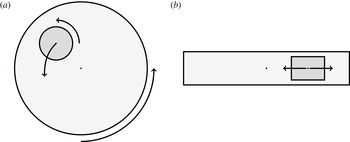
Our main motivation arises from a tissue engineering problem. One approach to in vitro tissue engineering is to seed cells onto a porous biomaterial scaffold, which is then cultured within a bioreactor. The combination of cells and scaffold is referred to as a tissue construct and one particular aim of tissue engineering is to make porous tissue constructs as permeable as possible whilst maintaining their structural integrity. This is to enhance nutrient delivery to the cells residing in the interior of the construct via advection. Moreover, many cells are mechanosensitive, and their proliferation rate depends on the stress that they experience. In a high aspect ratio vessel bioreactor, the porous tissue construct is placed within a bioreactor shaped like a Petri dish turned on its side, and the entire set-up is saturated with a nutrient-rich fluid, and rotated around the bioreactor axis (figure 1). The construct moves according to the force it experiences and, in the short term, the construct undergoes periodic motion. However, over a long time, the tissue construct drifts from its periodic orbit, an effect that can be attributed to weak inertia. To predict the construct trajectory and, ultimately, the nutrient transport in such a bioreactor, we must determine the forces acting on the construct. Thus, determining the flow through the porous construct is of particular importance. To gain insights into this problem, we consider the flow past a tissue construct held at a fixed position, with a particular view to investigating the effect of weak inertia. Such an analysis can then be used to determine the construct trajectory when it is free to move. Another application of interest is the interfacial erosion of a porous biofilm, which is proportional to the square root of the fluid shear stress evaluated at the interface (Duddu et al. Reference Duddu, Chopp and Moran2009). Thus, it is of interest to determine both the internal stress within the porous obstacle for tissue engineering applications and the interfacial stress acting on the obstacle boundary for biofilm erosion problems.
Schematic of a high aspect ratio vessel bioreactor, containing a porous scaffold (darker region). The bioreactor has a similar shape to a Petri dish turned on its side. (a) Face view. (b) Side view showing the gaps between the scaffold and the bioreactor. Cells are seeded within the scaffold, and the entire bioreactor is filled with a nutrient-rich fluid and rotated around its axis, causing the scaffold to move.

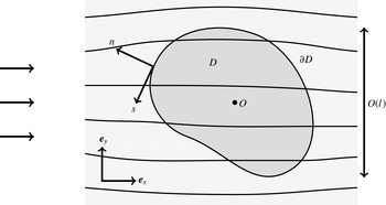
The main aim of this paper is to investigate steady laminar flow through a narrow two-dimensional channel blocked by a tightly fitting finite-length porous obstacle, and then to generalise this analysis to investigate a time-dependent three-dimensional flow past a porous cylinder with an arbitrary smooth cross-section within a Hele-Shaw cell, as illustrated in figure 2. In particular, we are interested in the behaviour of the flow near the interface between the single-phase and porous regions, governed by the Navier–Stokes and Darcy equations, respectively. Transition from plug to Poiseuille flow in a two-dimensional channel is a classic problem, with the asymptotic structure examined by Van Dyke (Reference Van Dyke1970) and Wilson (Reference Wilson1971), and numerical solutions given by, for example, Bodoia & Osterle (Reference Bodoia and Osterle1961) and Brandt & Gillis (Reference Brandt and Gillis1966). Although Van Dyke (Reference Van Dyke1970) mentions that a porous mesh would have to be used experimentally to induce uniform flow at the entry to a channel, the nature of the coupled flow between single-phase and porous regions remains an open question – one which we will answer in this paper.
The model geometry for flow within (a) a channel and (b) a Hele-Shaw cell. The light region is the exterior fluid and the dark region is the porous obstacle.

Thompson (Reference Thompson1968) used the method of matched asymptotic expansions to analyse the three-dimensional flow near a solid circular cylinder within a Hele-Shaw cell, exploiting the small aspect ratio of the cell. Due to the no-flux condition on the solid cylinder, the normal flow near the interface is small. We are motivated by the tissue engineering application in which there is flow within a highly permeable porous obstruction of arbitrary smooth cross-section. The normal flow, in general, is then significant near the interface and the flows inside and outside the obstacle are coupled through their boundary conditions at the interface. Although we are interested in a highly permeable obstacle, we do not consider the Brinkman extension to the Darcy equations in this paper because the porous construct must maintain its structural integrity. That is, we consider a porous medium whose underlying solid matrix is connected, so that Brinkman’s equations do not apply (Auriault Reference Auriault2009).
We shall make extensive use of the method of matched asymptotic expansions by exploiting the small aspect ratio of the channel/Hele-Shaw cell – one of our goals is to understand the flow near the interface (in an ‘inner’ region) given a general flow away from the interface (in an ‘outer’ region). Although the outer problems satisfy reduced equations, the inner problems are quasi-two-dimensional in each plane perpendicular to the interface. In particular, we determine the behaviour of inherently local properties, such as the stress acting on the interface. Additionally, we derive systematically the conditions that couple the outer equations for a general far-field forcing and for a general smooth cross-section of the porous obstacle. Due to their generality, the results obtained in this paper can significantly reduce the computational expense required to solve flow problems with coupled single-phase and porous regions, whilst retaining important interfacial information.
There is a large literature addressing the question of interfacial conditions on the boundary of a porous obstacle (and it remains an area of active research); see, for example, Nield & Bejan (Reference Nield and Bejan2006) for a comprehensive review. We do not address this question here, and use as our interfacial boundary conditions: continuity of flux and continuity of pressure, together with a no tangential slip condition. The first two are derived in Levy & Sanchez-Palencia (Reference Levy and Sanchez-Palencia1975), the last is a special case of the general tangential slip condition derived in Carraro et al. (Reference Carraro, Goll, Marciniak-Czochra and Mikelić2015).
The structure of this paper is as follows. In § 2, we consider the steady two-dimensional case of flow through a channel containing a tight-fitting highly permeable porous obstacle. In § 2.1, we formulate the mathematical problem. In § 2.3, we describe the asymptotic structure in the small aspect ratio limit and present the problems to be solved to couple the outer single-phase and porous regions. In §§ 2.4 and 2.5, we investigate the asymptotic behaviour of these coupling conditions in the small and large Reynolds number limits, respectively. In particular, we find that the large Reynolds number limit induces a further boundary layer structure, and we investigate this in full. In § 3 we extend our analysis to an unsteady three-dimensional flow in a Hele-Shaw cell past a tight-fitting highly permeable cylindrical porous obstacle. If the curvature of the cross-sectional boundary of the porous obstacle is not large (in a sense to be made precise later), the boundary layer structure in each plane perpendicular to the interface is equivalent to the two-dimensional case considered in § 2, and we are able to generalize the two-dimensional results to the three-dimensional case. In § 4 we apply the general results of § 3 to a time-dependent forced far-field flow in a Hele-Shaw cell containing a porous cylinder with circular cross-section. We determine the internal and interfacial stress within and on the porous construct, and show that fluid inertia can result in the generation of a net force on the cylinder, even when the far-field flow is periodic with zero mean. If the cylinder were allowed to move, this would cause a long-term drift, thus highlighting the singular perturbative nature of fluid inertia, and how it can be important in dynamical problems arising in lubrication flow.
2 Steady two-dimensional flow
2.1 Model formulation
We consider the steady two-dimensional flow of an incompressible Newtonian fluid with density
 ${\it\rho}$
and viscosity
 ${\it\mu}$
in an infinitely long channel of height
 $h$
. The channel contains a fully saturated porous obstacle with rectangular cross-section, height
 $h$
and length
 $2l$
, as illustrated in figure 2(a). The aspect ratio
 ${\it\epsilon}=h/l$
is assumed to be small. We use Cartesian coordinates
 $(x,z)$
along and across the channel, as illustrated in figure 2(a), such that in the channel
 $z\in [0,h]$
and the plug lies in
 $x\in [-l,l]$
,
 $z\in [0,h]$
. The flow is driven by a prescribed upstream pressure gradient, such that in the far field we have Poiseuille flow with cross-sectionally averaged velocity of magnitude
 $U_{av}$
.
The flow exterior to the porous plug (the light regions in figure 2
a), which we refer to as the ‘exterior flow’, is governed by the incompressible steady Navier–Stokes equations with no body force. The exterior fluid velocity, pressure, and stress tensor are denoted by
 $\boldsymbol{u}=u\boldsymbol{e}_{x}+w\boldsymbol{e}_{z}$
,
 $p$
, and
 $\boldsymbol{{\bf\sigma}}$
, respectively, where
 $\boldsymbol{e}_{x}$
and
 $\boldsymbol{e}_{z}$
are the unit vectors in the
 $x$
- and
 $z$
-directions, respectively. The fluid inside the porous plug (the dark region in figure 2
a), which we refer to as the ‘interior flow’, is governed by the incompressible Darcy equations, again with no body force. The Darcy (volume-averaged) velocity and (interstitial) pressure within the porous plug are denoted by
 $\boldsymbol{Q}=U\boldsymbol{e}_{x}+W\boldsymbol{e}_{z}$
and
 $P$
, respectively. The porous plug has constant permeability
 $k$
. We do not use the porosity of the plug as a parameter as it is absorbed into the definition of the volume-averaged velocity, but note that it is assumed to be constant.
We non-dimensionalize by setting
 $x=lx^{\prime }$
,
 $z={\it\epsilon}lz^{\prime }$
,
 $u=U_{av}u^{\prime }$
,
 $U=U_{av}U^{\prime }$
,
 $w={\it\epsilon}U_{av}w^{\prime }$
,
 $W={\it\epsilon}U_{av}W^{\prime }$
,
 $p=({\it\mu}U_{av}/({\it\epsilon}h))p^{\prime }$
,
 $P=({\it\mu}U_{av}/({\it\epsilon}h))P^{\prime }$
and
 $\boldsymbol{{\bf\sigma}}=({\it\mu}U_{av}/({\it\epsilon}h))\boldsymbol{{\bf\sigma}}^{\prime }$
, where primes denote dimensionless quantities. Since all variables are dimensionless henceforth, we drop the primes without risk of confusion.
The dimensionless governing equations in the exterior region
 $|x|>1$
,
 $0<z<1$
are the scaled Navier–Stokes equations given by
 $$\begin{eqnarray}\displaystyle & \displaystyle {\it\epsilon}Re(uu_{x}+wu_{z})=-p_{x}+u_{zz}+{\it\epsilon}^{2}u_{xx}, & \displaystyle\end{eqnarray}$$
 $$\begin{eqnarray}\displaystyle & \displaystyle {\it\epsilon}^{3}Re(uw_{x}+ww_{z})=-p_{z}+{\it\epsilon}^{2}w_{zz}+{\it\epsilon}^{4}w_{xx}, & \displaystyle\end{eqnarray}$$
 $$\begin{eqnarray}\displaystyle & \displaystyle 0=u_{x}+w_{z}, & \displaystyle\end{eqnarray}$$
 $Re={\it\rho}U_{av}h/{\it\mu}$
is the modified Reynolds number based on the channel height. The governing equations in the porous plug
 $|x|<1$
,
 $0<z<1$
are the scaled Darcy equations given by
 $$\begin{eqnarray}U=-KP_{x},\quad {\it\epsilon}^{2}W=-KP_{z},\quad 0=U_{x}+W_{z},\end{eqnarray}$$
where the dimensionless permeability
 $K=k/h^{2}$
. For the Darcy equations to be valid, we must have
 $K\ll 1$
. We discuss the typical sizes of the three dimensionless parameters appearing in our model,
 ${\it\epsilon}$
,
 $Re$
and
 $K$
, in § 2.2.
2.1.1 Boundary conditions
On the channel walls we impose no-flux and no-slip conditions on the exterior flow and a no-flux condition on the Darcy flow, so that
 $$\begin{eqnarray}\boldsymbol{u}=\mathbf{0}\quad \text{on }z=0,1\text{ for }|x|>1;\quad W=0\quad \text{on }z=0,1\text{ for }|x|<1.\end{eqnarray}$$
On the inflow (
 $x=-1$
) and outflow (
 $x=1$
) interfaces, continuity of flux, continuity of pressure and a no tangential slip condition (Levy & Sanchez-Palencia Reference Levy and Sanchez-Palencia1975; Carraro et al.
Reference Carraro, Goll, Marciniak-Czochra and Mikelić2015) are given by
 $$\begin{eqnarray}u=U,\quad p=P,\quad w=0\quad \text{on }x=\pm 1\text{ for }0<z<1.\end{eqnarray}$$
The flow is driven by imposing a constant, upstream pressure gradient in the far field, with
 $$\begin{eqnarray}\displaystyle \frac{\text{d}p}{\text{d}x}\rightarrow -12\quad \text{as }x\rightarrow -\infty , & & \displaystyle\end{eqnarray}$$
ensuring that the cross-sectionally averaged horizontal component of velocity has magnitude
 $1$
in the far field.
2.2 Parameter values
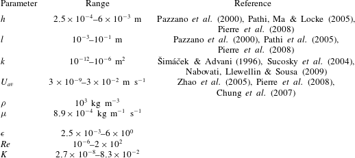
Within a bioreactor, values of the three dimensionless parameters
 ${\it\epsilon}$
,
 $Re$
and
 $K$
can vary greatly in magnitude (table 1). We will investigate the dimensionless problem defined by (2.1)–(2.5) in specific regions of this parameter space.
Typical dimensional parameter values and the corresponding values of the dimensionless parameters. The absolute upper bound of
 $1/12\approx 8.3\times 10^{-2}$
for
 $K$
can be obtained by considering unobstructed Poiseuille flow through a channel. We use the density and viscosity values of water at room temperature for
 ${\it\rho}$
and
 ${\it\mu}$
, respectively.

The dimensionless problem is characterised by two length scales: the obstacle half-length,
 $1$
, and the channel height,
 ${\it\epsilon}$
. We proceed by considering the case in which
 ${\it\epsilon}\ll 1$
, the channel height then being much smaller than the half-length of the obstacle.
The value of
 $K$
must be small enough for the underlying solid matrix to be connected, resulting in Darcy’s equations governing the flow within the porous medium (Auriault Reference Auriault2009), but large enough to enhance nutrient transfer via fluid advection to the cells within the plug. There is an absolute upper bound of
 $K<1/12$
, and this can be seen by considering unobstructed Poiseuille flow through a channel. In reality,
 $K\ll 1$
, and we work in this limit. We see in the three-dimensional case, considered in § 3, that
 $K=O({\it\epsilon})$
corresponds to an obstacle which is impermeable to the flow at leading order. Hence, this limit reduces to the leading-order problem given in Thompson (Reference Thompson1968), who considered the three-dimensional flow near a solid circular cylinder within a Hele-Shaw cell. We consider instead the limit in which
 ${\it\epsilon}\ll K\ll 1$
, corresponding to the regime in which the plug is long, thin and permeable at leading order in
 ${\it\epsilon}$
. Examples of long, thin tissues include skin (Lei et al.
Reference Lei, Ning, Cao, Liu, Zhang, Qiu, Hu, Zhang, Liu and Duan2011), urothelial tissue (Gabouev et al.
Reference Gabouev, Schultheiss, Mertsching, Köppe, Schlote, Wefer, Jonas and Stief2003) and the cornea (Su et al.
Reference Su, Hidaka, Kimura and Yamamoto2003). Although we do assume that
 $K\ll 1$
throughout this paper, we effectively treat
 $K=O(1)$
as
 ${\it\epsilon}\rightarrow 0$
in our following asymptotic analysis for mathematical expediency.
We must also define the relative scaling of
 $Re$
. There is a distinguished limit when
 $Re=O(1)$
, and the investigation of this limit is the subject of the next section. Further analytic progress can be made when
 $Re$
is either small or large: we consider the asymptotic sublimit
 $Re\ll 1$
in § 2.4, and the asymptotic sublimit
 $1\ll 1/K\ll Re\ll 1/{\it\epsilon}$
in § 2.5. We note that Darcy’s law (2.2) and the continuity of pressure condition (2.4b
) would require modification if we were to generalize this work to significantly larger Reynolds numbers (Kaviany Reference Kaviany2012).
2.3 Asymptotic structure for
 $Re=O(1)$

We seek a solution using the method of matched asymptotic expansions with small parameter
 ${\it\epsilon}$
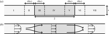
. The asymptotic structure is shown in figure 3(a), where each of seven asymptotic regions are labelled I–VII. We describe the regions as follows, noting that in each case the relevant transverse length scale is the channel height,
 ${\it\epsilon}$
. There are three ‘outer’ regions characterised by an
 $O(1)$
axial length scale: two for the exterior fluid (regions I and VII) in which we have Poiseuille flow at leading order, and one for the interior fluid (region IV) in which we have plug flow at leading order. Thus, there is a transition from Poiseuille to plug to Poiseuille flow, between regions I, IV and VII, respectively, as illustrated schematically in figure 3(b). The inflow transition from Poiseuille to plug flow occurs near the interface
 $x=-1$
, where there are two ‘inner’ regions, one on each side of the interface, each characterised by an axial length scale of
 $O({\it\epsilon})$
. The exterior inflow inner region is region II, and the porous inflow inner region is region III. In a similar manner, the outflow transition from plug to Poiseuille flow occurs near the interface
 $x=1$
, where again there are two inner regions, one on each side of the interface, and each characterised by an axial length scale of
 $O({\it\epsilon})$
. The porous outflow inner region is region V and the exterior outflow inner region is region VI.
The boundary layer structure for
 $Re=O(1)$
. The light region is the exterior fluid and the dark region is the porous obstacle. (a) The different asymptotic regions are indicated and labelled in Roman numerals. (b) A schematic representation of the flow.

2.3.1 Outer regions
In the outer regions I, IV and VII, we begin by posing asymptotic expansions of the form
 $$\begin{eqnarray}\displaystyle (\boldsymbol{u},\boldsymbol{Q},p,P)=(\boldsymbol{u}_{0},\boldsymbol{Q}_{0},p_{0},P_{0})+{\it\epsilon}(\boldsymbol{u}_{1},\boldsymbol{Q}_{1},p_{1},P_{1})+O({\it\epsilon}^{2})\quad \text{as }{\it\epsilon}\rightarrow 0. & & \displaystyle\end{eqnarray}$$
Substituting (2.6) into (2.1), we find that the leading-order governing equations for the exterior flow are simply the lubrication equations
 $$\begin{eqnarray}0=-p_{0x}+u_{0zz},\quad 0=-p_{0z},\quad 0=u_{0x}+w_{0z}\quad \text{for }|x|>1,0<z<1.\end{eqnarray}$$
Substituting (2.6) into (2.2), the leading-order governing equations for the interior flow are
 $$\begin{eqnarray}U_{0}=-KP_{0x},\quad 0=-KP_{0z},\quad 0=U_{0x}+W_{0z}\quad \text{for }|x|<1,0<z<1.\end{eqnarray}$$
At leading-order, the channel wall boundary conditions (2.3) become
 $$\begin{eqnarray}\displaystyle & \displaystyle \boldsymbol{u}_{0}=\mathbf{0}\quad \text{on }z=0,1\text{ for }|x|>1, & \displaystyle\end{eqnarray}$$
 $$\begin{eqnarray}\displaystyle & \displaystyle W_{0}=0\quad \text{on }z=0,1\text{ for }|x|<1, & \displaystyle\end{eqnarray}$$
 $$\begin{eqnarray}\displaystyle \frac{\text{d}p_{0}}{\text{d}x}\rightarrow -12\quad \text{as }x\rightarrow -\infty . & & \displaystyle\end{eqnarray}$$
We are unable to impose at leading-order the interfacial boundary conditions (2.4) in the outer regions; these conditions are satisfied within the inner regions described in § 2.3.2. For the outer problems, we must instead impose matching conditions (using the matching law given in Van Dyke (Reference Van Dyke1975)). These are determined in § 2.3.2, and we state them here to close the leading-order outer problem. As the outer pressure is independent of
 $z$
and the fluid velocity is proportional to the pressure gradient, we find that we may impose continuity of total flux and pressure at each interface (corresponding to Neumann and Dirichlet conditions on the pressure, respectively). That is,
 $$\begin{eqnarray}\int _{0}^{1}u_{0}\,\text{d}z=\int _{0}^{1}U_{0}\,\text{d}z,\quad p_{0}=P_{0}\quad \text{on }x=\pm 1.\end{eqnarray}$$
We note that whilst the conditions (2.11) close the outer problem, they give no information about, for example, the leading-order stress acting on the interfaces.
The leading-order solutions are readily obtained as follows: in region I,
 $$\begin{eqnarray}\boldsymbol{u}_{0}=6z(1-z)\boldsymbol{e}_{x},\quad p_{0}=-12x;\end{eqnarray}$$
in region IV,
 $$\begin{eqnarray}\boldsymbol{U}_{0}=\boldsymbol{e}_{x},\quad P_{0}=-\frac{1+x}{K}+12;\end{eqnarray}$$
and in region VII,
 $$\begin{eqnarray}\boldsymbol{u}_{0}=6z(1-z)\boldsymbol{e}_{x},\quad p_{0}=-12x+\left(24-\frac{2}{K}\right).\end{eqnarray}$$
The pressure is determined up to an arbitrary constant which (at this order) we fix by supposing
 $p_{0}+12x\rightarrow 0$
as
 $x\rightarrow -\infty$
, without loss of generality. We remark that the presence of the porous plug introduces a jump in pressure of
 $24-2/K\sim -2/K$
(as
 $K$
is small). Equivalently, an
 $O(1)$
pressure drop creates an
 $O(K)$
flow through the porous plug.
We note that the horizontal components of velocity (2.12a ) and (2.13a ) are incompatible with the continuity of flux condition (2.4a ) on the interfacial inflow boundary for the full problem. Similarly for outflow, we find that (2.13a ) and (2.14a ) are incompatible with (2.4a ). In the next section we introduce inner regions to resolve this issue, but for the remainder of this section we consider higher-order terms in the outer regions as the higher-order pressure is coupled to the leading-order flow in the inner regions.
Using the leading-order solutions (2.12) and (2.14), the
 $O({\it\epsilon})$
terms in the governing equations for the exterior flow (2.1) become
 $$\begin{eqnarray}0=-p_{1x}+u_{1zz},\quad 0=-p_{1z},\quad 0=u_{1x}+w_{1z}\quad \text{for }|x|>1,0<z<1.\end{eqnarray}$$
Similarly, using the leading-order solutions (2.13), the
 $O({\it\epsilon})$
terms in the governing equations for the interior flow (2.2) become
 $$\begin{eqnarray}U_{1}=-KP_{1x},\quad 0=-KP_{1z},\quad 0=U_{1x}+W_{1z}\quad \text{for }|x|<1,0<z<1.\end{eqnarray}$$
The channel wall boundary conditions (2.3) at this order are as follows
 $$\begin{eqnarray}\displaystyle & \displaystyle \boldsymbol{u}_{1}=\mathbf{0}\quad \text{on }z=0,1\text{ for }|x|>1, & \displaystyle\end{eqnarray}$$
 $$\begin{eqnarray}\displaystyle & \displaystyle W_{1}=0\quad \text{on }z=0,1\text{ for }|x|<1, & \displaystyle\end{eqnarray}$$
 $$\begin{eqnarray}\displaystyle \frac{\text{d}p_{1}}{\text{d}x}\rightarrow 0\quad \text{as }x\rightarrow -\infty . & & \displaystyle\end{eqnarray}$$
The matching conditions across each interface are determined in § 2.3.2, and we give them here to close the problem. For inflow, we have
 $$\begin{eqnarray}\int _{0}^{1}u_{1}\,\text{d}z=\int _{0}^{1}U_{1}\,\text{d}z,\quad p_{1}-P_{1}={\it\Pi}^{-}(Re,K)\quad \text{on }x=-1,\end{eqnarray}$$
and for outflow we have
 $$\begin{eqnarray}\int _{0}^{1}u_{1}\,\text{d}z=\int _{0}^{1}U_{1}\,\text{d}z,\quad p_{1}-P_{1}={\it\Pi}^{+}(Re,K)\quad \text{on }x=1,\end{eqnarray}$$
where the pressure jumps
 ${\it\Pi}^{-}$
and
 ${\it\Pi}^{+}$
are functions of the parameters
 $Re$
and
 $K$
. In § 2.3.2, we specify the problems that need to be solved to determine these functions, while in §§ 2.4 and 2.5 we determine their asymptotic behaviour for small and large
 $Re$
.
Given
 ${\it\Pi}^{\pm }$
, the solution to (2.15)–(2.20) is readily determined: in region I,
 $$\begin{eqnarray}\boldsymbol{u}_{1}=\mathbf{0},\quad p_{1}={\it\Pi}^{-};\end{eqnarray}$$
in region IV,
 $$\begin{eqnarray}\boldsymbol{Q}_{1}=\mathbf{0},\quad P_{1}=0;\end{eqnarray}$$
and in region VII,
 $$\begin{eqnarray}\boldsymbol{u}_{1}=\mathbf{0},\quad p_{1}={\it\Pi}^{+}.\end{eqnarray}$$
As with the leading-order solutions (2.12)–(2.14), the pressure field is unique up to an arbitrary constant. For convenience, we choose the constant such that
 $P_{1}(0,0.5)=0$
, without loss of generality. We proceed by considering the inner regions, highlighting the problems that would need to be solved numerically to determine the functions
 ${\it\Pi}^{-}$
and
 ${\it\Pi}^{+}$
.
2.3.2 Inner regions
The appropriate scalings in the inflow and outflow inner regions are
 $x=\mp 1+{\it\epsilon}X^{\mp }$
, respectively, with
 $(w,W)=(\overline{w},\overline{W})/{\it\epsilon}$
. To make it clear that we are working in the inner regions we introduce overbars on the other dimensionless variables, writing
 $(u,U)=(\overline{u},\overline{U})$
,
 $(p,P)=(\overline{p},\overline{P})$
and
 $(\overline{\boldsymbol{u}},\overline{\boldsymbol{Q}})=(\overline{u},\overline{U})\boldsymbol{e}_{x}+(\overline{w},\overline{W})\boldsymbol{e}_{z}$
. Using vector operators in terms of
 $X^{\mp }$
and
 $z$
as appropriate, the exterior fluid governing equations (2.1) become
 $$\begin{eqnarray}Re(\overline{\boldsymbol{u}}\boldsymbol{\cdot }\boldsymbol{{\rm\nabla}})\overline{\boldsymbol{u}}=-{\it\epsilon}^{-1}\boldsymbol{{\rm\nabla}}\overline{p}+{\rm\nabla}^{2}\overline{\boldsymbol{u}},\quad 0=\boldsymbol{{\rm\nabla}}\boldsymbol{\cdot }\overline{\boldsymbol{u}}\quad \text{in regions II and VI},\end{eqnarray}$$
which are valid when
 $X^{-}<0$
for inflow (region II) and
 $X^{+}>0$
for outflow (region VI), with
 $0<z<1$
in both cases. The interior fluid governing equations (2.2) become
 $$\begin{eqnarray}\overline{\boldsymbol{Q}}=-{\it\epsilon}^{-1}K\boldsymbol{{\rm\nabla}}\overline{P},\quad 0=\boldsymbol{{\rm\nabla}}\boldsymbol{\cdot }\overline{\boldsymbol{Q}}\quad \text{in regions III and V},\end{eqnarray}$$
which are valid for
 $X^{-}>0$
for inflow (region III) and
 $X^{+}<0$
for outflow (region V), with
 $0<z<1$
in both cases.
Similarly to (2.6), we form inner expansions in powers of
 ${\it\epsilon}$
as follows:
 $$\begin{eqnarray}\displaystyle (\overline{\boldsymbol{u}},\overline{\boldsymbol{Q}},\overline{p},\overline{P})=(\overline{\boldsymbol{u}}_{0},\overline{\boldsymbol{Q}}_{0},\overline{p}_{0},\overline{P}_{0})+{\it\epsilon}(\overline{\boldsymbol{u}}_{1},\overline{\boldsymbol{Q}}_{1},\overline{p}_{1},\overline{P}_{1})+O({\it\epsilon}^{2})\quad \text{as }{\it\epsilon}\rightarrow 0. & & \displaystyle\end{eqnarray}$$
At leading order, it follows from (2.24a ) that
 $$\begin{eqnarray}\displaystyle \mathbf{0}=-\boldsymbol{{\rm\nabla}}\overline{p}_{0}\quad \text{in regions II and VI}, & & \displaystyle\end{eqnarray}$$
while (2.25a ) gives, similarly,
 $$\begin{eqnarray}\displaystyle \mathbf{0}=-K\boldsymbol{{\rm\nabla}}\overline{P}_{0}\quad \text{in regions III and V}. & & \displaystyle\end{eqnarray}$$
The appropriate interfacial conditions on
 $X^{\mp }=0$
for the leading-order pressure are given by the leading-order terms in (2.4b
), which become
 $$\begin{eqnarray}\displaystyle \overline{p}_{0}=\overline{P}_{0}\quad \text{on }X^{\mp }=0. & & \displaystyle\end{eqnarray}$$
Thus
 $p_{0}$
and
 $P_{0}$
are constant and equal in regions II and III and in regions V and VI, leading to the matching condition (2.11b
). Using the leading-order outer solutions (2.12)–(2.14) for the pressure, we find
 $$\begin{eqnarray}\overline{p}_{0}=12\quad \text{in region II},\quad \overline{P}_{0}=12\quad \text{in region III},\end{eqnarray}$$
for inflow, and
 $$\begin{eqnarray}\overline{P}_{0}=12-\frac{2}{K}\quad \text{in region V},\quad \overline{p}_{0}=12-\frac{2}{K}\quad \text{in region VI}\end{eqnarray}$$
for outflow. We note that these leading-order pressures are constant on the interface, as predicted by Levy & Sanchez-Palencia (Reference Levy and Sanchez-Palencia1975).
As the leading-order fluid pressures are constant within each inner region, the leading-order inner flow is driven by the first correction to pressure, and these equations are given by the
 $O(1)$
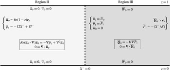
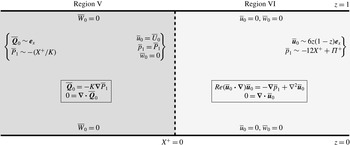
terms in (2.24) and (2.25). We illustrate the leading-order flow problems in figure 4 for inflow, and in figure 5 for outflow. In both cases, the inner flow transition problem is governed by the two-dimensional steady Navier–Stokes equations coupled to the Darcy equations. To fully determine the inflow and outflow pressure jumps
 ${\it\Pi}^{-}$
and
 ${\it\Pi}^{+}$
, we would have to solve the problems indicated in figures 4 and 5 numerically for two parameters:
 $Re$
and
 $K$
.
The inner inflow problem for
 $Re=O(1)$
. The flow is from left to right.

The inner outflow problem for
 $Re=O(1)$
. The flow is from left to right.

However, to couple the outer regions, we require another condition on the pressure. We note that we can analytically determine suitable coupling conditions for the horizontal components of velocity averaged over the channel height by appealing to global conservation of mass, rather than solving the full problem. By integrating the continuity equations across the channel height, using the conditions for the flow in the normal direction at each boundary and matching with the outer solutions, we deduce the following coupling conditions for the outer horizontal components of velocity
 $$\begin{eqnarray}\int _{0}^{1}u_{0}\,\text{d}z=\int _{0}^{1}U_{0}\,\text{d}z,\quad \int _{0}^{1}u_{1}\,\text{d}z=\int _{0}^{1}U_{1}\,\text{d}z\quad \text{on }x=\pm 1.\end{eqnarray}$$
We proceed by determining the inner flow in the asymptotic sublimits
 $Re\ll 1$
and
 $1\ll 1/K\ll Re\ll 1/{\it\epsilon}$
, starting with the former. This will allow us to calculate quantities that are unobtainable from sole consideration of the outer problem, such as the stress acting on the interface and the limiting behaviour of the functions
 ${\it\Pi}^{-}$
,
 ${\it\Pi}^{+}$
.
2.4 Small Reynolds number:
$Re\ll 1$

In the sublimit in which
 $Re\ll 1$
, the leading-order problems outlined in figures 4 and 5 become Stokes flow coupled with Darcy flow. Therefore, the flow equations are now reversible, and it suffices to solely consider inflow. We therefore use
 $X^{-}=X$
for ease of notation. Further, we note that the inflow and outflow pressure jumps are now linked via the expression
 ${\it\Pi}^{+}=-{\it\Pi}^{-}$
.
We solve the resulting leading-order system numerically (for the streamfunction within the exterior flow and for the pressure within the porous flow) using a second-order accurate central finite-difference scheme. Due to the elliptic nature of the governing equations, we use an iterative method to bypass some of the cost of solving the fully coupled elliptic problems in one step. That is, we iterate between solving Laplace’s equation for the pressure in region III, and the biharmonic equation for the streamfunction in region II, and use the solution found in the previous iteration to determine the boundary conditions for the current iteration. We truncate the infinite domain to
 $[-1,0]$
for
 $X$
in region II and
 $[0,1]$
for
 $X$
in region III (we note that an extended domain adds little accuracy to the scheme), using 300 grid points for
 $X$
in each region and 300 grid points for
 $z$
. The simulation is halted once the difference between successive iterations at each grid point is less than
 $10^{-4}$
.
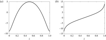
The normal and shear components of stress acting on the interface are
 $$\begin{eqnarray}\displaystyle & \displaystyle {\it\sigma}_{xx}\sim -12+{\it\epsilon}(-\overline{p}_{1}+2\overline{u}_{0X}), & \displaystyle\end{eqnarray}$$
 $$\begin{eqnarray}\displaystyle & \displaystyle {\it\sigma}_{xz}\sim {\it\epsilon}(\overline{u}_{0z}+\overline{w}_{0X}), & \displaystyle\end{eqnarray}$$
 ${\it\epsilon},Re\rightarrow 0$
. We show the
 $O({\it\epsilon})$
stress results for
 $K=0.01$
in figure 6, and calculate
 ${\it\Pi}^{-}=1.92$
to three significant figures. The leading-order normal stress term in (2.33a
) takes the specific value of
 $-12$
because we have imposed
 $P(0,z)=0$
to uniquely define the pressure. In fact, it is the
 $O({\it\epsilon})$
terms in (2.33) which are more interesting, as these are the dominant terms which vary in
 $z$
and, unlike the leading-order pressure, cannot simply be determined from the outer solution. Hence, the boundary layer analysis is essential to obtain these results. The reason the outer solutions cannot make good predictions of the
 $z$
-variation of interfacial stress is because of the tendency of the exterior flow to move towards the channel edges in transition between Poiseuille and plug flow in the boundary region. The interfacial normal stress is greater/smaller than predicted by the outer flow towards the centre/edges of the channel, whilst the magnitude of interfacial shear stress is greater than predicted by the outer solution.
The
 $O({\it\epsilon})$
normal and shear stresses acting on the interface
 $X=0$
, for
 $K=0.01$
. (a)
 $\overline{p}_{1}-2\overline{u}_{0X}$
, (b)
 $-(\overline{u}_{0z}+\overline{w}_{0X})$
.

2.5 Large Reynolds number:
$1\ll 1/K\ll Re\ll 1/{\it\epsilon}$

We now consider the sublimit in which
 $1\ll 1/K\ll Re\ll 1/{\it\epsilon}$
. We do not consider further the sublimits in which
 $ReK=O(1)$
or
 $1\ll Re\ll 1/K\ll 1/{\it\epsilon}$
. This is because we are interested in the tissue engineering problem with porous plugs whose values of
 $K$
are not too small. Moreover, the above sublimits yield coupled nonlinear problems which are not amenable to analytic study. We emphasize that the limit we consider is when the external fluid has a large Reynolds number, but the pore Reynolds number is small, so that the Darcy equations and continuity of pressure conditions are valid.
In this section we perform an asymptotic analysis using the small parameter
 ${\it\delta}=1/Re\ll 1$
for ease of notation. Therefore, when we refer to, for example, ‘leading order’ in this section, it is meant in reference to
 ${\it\delta}$
. In the limit
 ${\it\delta}\rightarrow 0$
, there is a significant change in boundary layer structure within the inner regions II and VI compared to the
 $O(1)$
Reynolds number case. The limit as
 ${\it\delta}\rightarrow 0$
is singular, and we expect viscous effects to become important in regions near each boundary. Furthermore, as fluid momentum dominates within regions II and VI, the flow direction is important. Indeed, we obtain a different boundary layer structure for inflow and outflow, and therefore split the analysis into these two cases, starting with inflow.
In the limit of small
 ${\it\delta}$
, the first-correction terms
 $\boldsymbol{u}_{1}$
,
 $\boldsymbol{Q}_{1}$
,
 $p_{1}$
and
 $P_{1}$
from the asymptotic series in the outer regions (2.6) are now scaled with
 ${\it\delta}^{-1}$
to be consistent with the new inner scalings, as follows:
 $$\begin{eqnarray}\displaystyle (\boldsymbol{u}_{1},\boldsymbol{Q}_{1},p_{1},P_{1})={\it\delta}^{-1}(\boldsymbol{u}_{10},\boldsymbol{Q}_{10},p_{10},P_{10})+(\boldsymbol{u}_{11},\boldsymbol{Q}_{11},p_{11},P_{11})+O({\it\delta}). & & \displaystyle\end{eqnarray}$$
The scalings for the pressure jumps
 ${\it\Pi}^{-}$
and
 ${\it\Pi}^{+}$
will turn out to be
 $$\begin{eqnarray}{\it\Pi}^{-}={\it\Pi}_{1}^{-}+O({\it\delta}),\quad {\it\Pi}^{+}={\it\delta}^{-1}{\it\Pi}_{0}^{+}+O(1)\quad \text{as }{\it\delta}\rightarrow 0,\end{eqnarray}$$
our objective being to determine
 ${\it\Pi}_{1}^{-}$
and
 ${\it\Pi}_{0}^{+}$
.
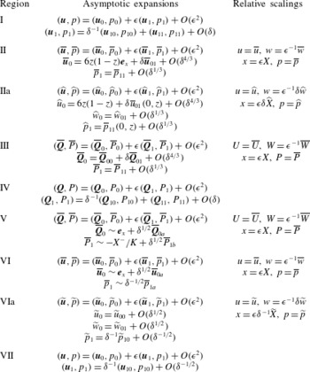
Though we have not yet fully described the inner asymptotic structure, we give the form of the asymptotic expansions within each region in table 2 for ease of reference.
Asymptotic expansions within boundary layers in the large Reynolds number limit.

2.5.1 Inflow
The inflow inner problem (within regions II and III) is shown in figure 4. The limit as
 ${\it\delta}\rightarrow 0$
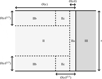
yields leading-order inviscid flow in region II away from the boundaries, with five additional boundary layers being required to satisfy all of the boundary conditions. Two of these viscous boundary layers are on the channel walls, one is on the porous interface, whilst the remaining boundary layers occur in the corners between the channel wall and porous interface. The boundary layer structure for the inflow problem is shown in figure 7.
Schematic diagram of the inner regions IIa–c within the inflow boundary region II. The light region is the exterior fluid and the dark region is the porous obstacle. The size of the boundary layers has been exaggerated for illustrative purposes.

We start by considering the coupled regions II and III, and show that the transition to Poiseuille flow occurs solely within region III at leading order in
 ${\it\delta}$
.
2.5.2 Regions II and III
Within regions II and III, we make the following asymptotic expansions
 $$\begin{eqnarray}\displaystyle & \displaystyle \overline{\boldsymbol{u}}_{0}=6z(1-z)\boldsymbol{e}_{x}+{\it\delta}\overline{\boldsymbol{u}}_{01}+{\it\delta}^{4/3}\overline{\boldsymbol{u}}_{02}+O({\it\delta}^{5/3}), & \displaystyle\end{eqnarray}$$
 $$\begin{eqnarray}\displaystyle & \displaystyle \overline{\boldsymbol{Q}}_{0}=\overline{\boldsymbol{Q}}_{00}+{\it\delta}\overline{\boldsymbol{Q}}_{01}+{\it\delta}^{4/3}\overline{\boldsymbol{Q}}_{02}+O({\it\delta}^{5/3}), & \displaystyle\end{eqnarray}$$
 $$\begin{eqnarray}\displaystyle & \displaystyle (\overline{p}_{1},\overline{P}_{1})=(\overline{p}_{11},\overline{P}_{11})+{\it\delta}^{1/3}(\overline{p}_{12},\overline{P}_{12})+O({\it\delta}^{2/3}) & \displaystyle\end{eqnarray}$$
 ${\it\delta}\rightarrow 0$
, where the non-integer powers of
 ${\it\delta}$
come from corrections to the flow that arise due to the presence of a boundary layer near the channel walls (regions IIb in figure 7). These terms are used in appendix A, but are not required further in this section.
Substituting the asymptotic expansions (2.36) into the governing equations presented in figure 4, the
 $O(1/{\it\delta})$
terms in region II are trivially satisfied, but so far
 $\overline{\boldsymbol{Q}}_{00}$
is unknown. Proceeding with the expansions, we find at
 $O(1)$
that
 $\overline{\boldsymbol{u}}_{01}=(\overline{u}_{01},\overline{w}_{01})$
is governed by
 $$\begin{eqnarray}\overline{u}_{00}\overline{u}_{01X}+\overline{u}_{00z}\overline{w}_{01}=-\overline{p}_{11X}-12,\quad \overline{u}_{00}\overline{w}_{01X}=-\overline{p}_{11z},\quad \boldsymbol{{\rm\nabla}}\boldsymbol{\cdot }\overline{\boldsymbol{u}}_{01}=0\quad \text{in region II},\end{eqnarray}$$
where
 $\overline{u}_{00}=6z(1-z)$
, while
 $\overline{\boldsymbol{Q}}_{00}=(\overline{U}_{00},\overline{W}_{00})$
is governed by
 $$\begin{eqnarray}\overline{\boldsymbol{Q}}_{00}=-K\boldsymbol{{\rm\nabla}}\overline{P}_{11},\quad 0=\boldsymbol{{\rm\nabla}}\boldsymbol{\cdot }\overline{\boldsymbol{Q}}_{00}\quad \text{in region III}.\end{eqnarray}$$
The boundary conditions we impose at this order in region II are again obtained via matching. On the channel walls (via matching with region IIb in appendix A), we have no flux, so that
 $$\begin{eqnarray}\displaystyle \overline{w}_{01}=0\quad \text{on }z=0,1\text{ for }X^{-}<0, & & \displaystyle\end{eqnarray}$$
while in the far field we match with region I, to obtain
 $$\begin{eqnarray}\overline{\boldsymbol{u}}_{01}\rightarrow \mathbf{0},\quad \overline{p}_{11}\sim -12X^{-}+{\it\Pi}_{1}^{-}\quad \text{as }X^{-}\rightarrow -\infty ~\text{for }0<z<1.\end{eqnarray}$$
Similarly, the boundary conditions in region III are
 $$\begin{eqnarray}\displaystyle \overline{W}_{00}=0\quad \text{on }z=0,1\text{ for }X^{-}>0, & & \displaystyle\end{eqnarray}$$
while matching with region IV gives
 $$\begin{eqnarray}\displaystyle \overline{P}_{11}\sim -\frac{X^{-}}{K}\quad \text{as }X^{-}\rightarrow \infty ~\text{for }0<z<1. & & \displaystyle\end{eqnarray}$$
We note that the far-field matching condition
 $\overline{\boldsymbol{Q}}_{00}\sim \boldsymbol{e}_{x}$
as
 $X^{-}\rightarrow \infty$
follows consistently from (2.42) using (2.38a
).
The interfacial conditions at
 $X^{-}=0$
for (2.37)–(2.38) are formally derived from consideration of the inner–inner boundary layer (region IIa) in § 2.5.3, within which we are able to satisfy the no tangential slip condition, but additionally find that the leading-order flow and the first correction to the pressure
 $\overline{p}_{11}$
are unchanged. From § 2.5.3, the correct conditions to couple regions II and III are continuity of flux and pressure, with
 $$\begin{eqnarray}6z(1-z)=\overline{U}_{00},\quad \overline{p}_{11}=\overline{P}_{11}\quad \text{on }X^{-}=0\text{ for }0<z<1.\end{eqnarray}$$
The system to solve in regions II and III (up to the
 $O({\it\delta})$
terms) is given by (2.37)–(2.43). We see that regions II and III have decoupled: the boundary condition (2.43a
) allows us to solve for
 $\overline{\boldsymbol{Q}}_{00}$
and
 $\overline{P}_{11}$
using (2.38) with (2.41)–(2.42), and then we can use the boundary condition (2.43b
) to determine
 $\overline{\boldsymbol{u}}_{01}$
and
 $\overline{p}_{11}$
using (2.37) with (2.39)–(2.40). The governing equations (2.38), with boundary conditions (2.41)–(2.42) and (2.43a
), are solved by
 $$\begin{eqnarray}\displaystyle -K\overline{P}_{11}=X^{-}+\mathop{\sum }_{k=1}^{\infty }A_{k}\exp (-2k{\rm\pi}X^{-})\cos (2k{\rm\pi}z),\quad A_{k}=\frac{3}{({\rm\pi}k)^{3}}. & & \displaystyle\end{eqnarray}$$
Since
 $\overline{\boldsymbol{u}}_{00}$
is independent of
 $X^{-}$
within region II, the leading-order transition from Poiseuille to plug flow occurs entirely within the porous medium in region III, and is governed by (2.44).
We now complete the solution in region II by determining
 $\overline{u}_{01}$
and
 $\overline{p}_{11}$
. As well as allowing us to determine
 ${\it\Pi}_{1}^{-}$
, knowledge of
 $\overline{p}_{11}$
gives the normal stress acting on the interface up to
 $O({\it\epsilon})$
, the first order at which the stress varies in the
 $z$
-direction. A rearrangement of the exterior flow (2.37) allows us to decouple the region II system (where
 $-\infty <X^{-}<0$
and
 $0<z<1$
) into
 $$\begin{eqnarray}\displaystyle & \displaystyle z(1-z){\rm\nabla}^{2}\overline{w}_{01}+2\overline{w}_{01}=0, & \displaystyle\end{eqnarray}$$
 $$\begin{eqnarray}\displaystyle & \displaystyle {\rm\nabla}^{2}\overline{p}_{11}=-2\overline{u}_{00z}\overline{w}_{01X^{-}}. & \displaystyle\end{eqnarray}$$
We solve (2.45a
) for
 $\overline{w}_{01}$
first, using boundary conditions (2.39) on
 $z=0$
,
 $1$
and (2.40a
) as
 $X^{-}\rightarrow -\infty$
. We derive a consistent boundary condition for
 $\overline{w}_{01}$
on
 $X^{-}=0$
using the boundary condition (2.43b
) for the pressure on
 $X^{-}=0$
, in combination with the governing equation (2.37b
), giving
 $$\begin{eqnarray}\displaystyle \overline{w}_{01X^{-}}=-\frac{1}{K\overline{u}_{00}}\mathop{\sum }_{k=1}^{\infty }2k{\rm\pi}A_{k}\sin (2k{\rm\pi}z)\quad \text{on }X^{-}=0\text{ for }0<z<1. & & \displaystyle\end{eqnarray}$$
The boundary condition (2.46) ensures that
 $\overline{w}_{01}$
does not vanish on
 $X^{-}=0$
, inducing a slip velocity on this interface within region II. This issue is taken care of in an inner–inner boundary layer closer to the interface (region IIa in figure 7) in § 2.5.3. The linearity of the governing equation (2.45a
), with boundary conditions (2.39), (2.40a
) and (2.46), also allows us to deduce that
 $\overline{w}_{01}$
scales with
 $K^{-1}$
. Further, from the continuity equation (2.37c
) it follows that
 $\overline{u}_{01}$
also scales with
 $K^{-1}$
.
We solve for
 $\overline{w}_{01}$
using a standard central finite-difference scheme. By numerically integrating
 $\overline{w}_{01}$
with respect to
 $X^{-}$
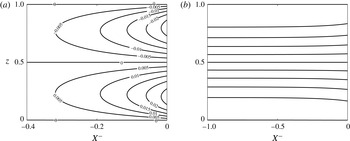
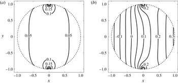
, we are able to plot the streamlines in figure 8. In figure 8(a), we show the streamlines for the first correction to the velocity, and in figure 8(b), we show the streamlines for the full velocity up to this first correction. We see that the fluid moves from the centre of the channel towards the channel walls, as expected. Therefore, adjustment from Poiseuille to plug flow occurs in region II, but at higher order. This movement induces a horizontal slip velocity on the channel walls, which is resolved in appendix A by introducing a boundary layer near the channel walls in which
 $z=O({\it\delta}^{1/3})$
on the bottom wall, with a similar layer near the top wall. These regions are labelled as IIb in figure 7. In appendix A, we show that the flow near
 $z=0$
has the form
 $$\begin{eqnarray}\displaystyle \overline{u}_{0}\sim 6z(1-z)+{\it\delta}\mathop{\sum }_{k=1}^{\infty }C_{k}\exp ({\it\mu}_{k}X^{-})g_{k}^{\prime }(0)\frac{\displaystyle \int _{0}^{z/{\it\delta}^{1/3}}\text{Ai}(a_{k}v)\,\text{d}v}{\displaystyle \int _{0}^{\infty }\text{Ai}(a_{k}s)\,\text{d}s}\quad \text{as }z\rightarrow 0^{+}, & & \displaystyle\end{eqnarray}$$
where
 $C_{k}$
,
 ${\it\mu}_{k}$
, and
 $g_{k}$
are described in (A1)–(A 2),
 $\text{Ai}$
is the Airy function of the first kind and
 $a_{k}$
is defined below (A 10). From (2.47), we see that the leading-order solution is preserved near the channel wall. In fact, the slip is resolved within higher-order terms in the boundary layer, and does not affect the leading-order solution in region II.
The streamlines for inflow near the interface. (a) The streamlines for the scaled first-correction velocity
 $K\overline{\boldsymbol{u}}_{01}$
, which is independent of
 $K$
. The fluid moves from the centre of the channel to the channel walls. (b) The streamlines for the full velocity up to first correction
 $\overline{\boldsymbol{u}}_{00}+{\it\delta}\overline{\boldsymbol{u}}_{01}$
(with a large value of
 ${\it\delta}/K=1$
taken to emphasise the effect of the correction). The fluid moves from left to right.

The problem for
 $\overline{p}_{11}$
is given by (2.45b
) with boundary conditions (2.40b
) and (2.43b
). We obtain consistent boundary conditions for
 $\overline{p}_{11}$
on the channel walls by substituting the leading-order flow solution into the governing equation (2.37b
) to obtain
 $$\begin{eqnarray}\displaystyle \overline{p}_{11z}=0\quad \text{on }z=0,1\text{ for }X^{-}<0. & & \displaystyle\end{eqnarray}$$
We solve the full system for
 $\overline{p}_{11}$
, given by (2.45b
) with boundary conditions (2.40b
), (2.43b
), and (2.48) numerically using a central finite-difference scheme. Using a similar scaling argument as for
 $\overline{w}_{01}$
, we find that
 ${\it\Pi}_{1}^{-}$
scales with
 $1/K$
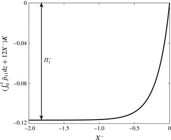
. We are able to calculate
 ${\it\Pi}_{1}^{-}$
by plotting
 $(\overline{p}_{11}+12X^{-})K$
, and using the matching condition (2.40b
). As
 ${\it\Pi}_{1}^{-}$
is independent of
 $z$
, and to more easily show the pressure drop on a graph, we plot
 $(\int _{0}^{1}\overline{p}_{11}\,\text{d}z+12X^{-})K$
for varying
 $X^{-}$
in figure 9. We find thereby that
 ${\it\Pi}_{1}^{-}={\it\alpha}/K$
, where
 ${\it\alpha}=-0.117$
to three significant figures.
The function
 $(\int _{0}^{1}\overline{p}_{11}\,\text{d}z+12X^{-})K$
for varying
 $X^{-}$
in region II, which allows us to determine the outer pressure drop for inflow.

2.5.3 Inner–inner region IIa
We now investigate the inner–inner boundary layer closer to the interface, region IIa in figure 7. This boundary layer is required to satisfy the no tangential slip condition on the interface, and captures a balance between the relevant inertial terms and the viscous terms induced by the presence of the porous interface.
The relevant scalings are
 $X^{-}={\it\delta}\widehat{X}$
and
 $\overline{w}_{0}={\it\delta}\widehat{w}_{0}$
, and we introduce the new variables
 $\overline{u}_{0}=\widehat{u}_{0}$
and
 $\overline{p}_{1}=\widehat{p}_{1}$
to signify that we are working in region IIa. Under these scalings, in region IIa (where
 $-\infty <\widehat{X}<0$
and
 $0<z<1$
) the exterior flow equations in figure 4 become
 $$\begin{eqnarray}\displaystyle & \displaystyle {\it\delta}^{-1}\widehat{u}_{0}\widehat{u}_{0\widehat{X}}+{\it\delta}\widehat{w}_{0}\widehat{u}_{0z}=-\widehat{p}_{1\widehat{X}}+{\it\delta}^{-1}\widehat{u}_{0\widehat{X}\widehat{X}}+{\it\delta}\widehat{u}_{0zz}, & \displaystyle\end{eqnarray}$$
 $$\begin{eqnarray}\displaystyle & \displaystyle \widehat{u}_{0}\widehat{w}_{0\widehat{X}}+{\it\delta}^{2}\widehat{w}_{0}\widehat{w}_{0z}=-{\it\delta}\widehat{p}_{1z}+\widehat{w}_{0\widehat{X}\widehat{X}}+{\it\delta}^{2}\widehat{w}_{0zz}, & \displaystyle\end{eqnarray}$$
 $$\begin{eqnarray}\displaystyle & \displaystyle 0=\widehat{u}_{0\widehat{X}}+{\it\delta}^{2}\widehat{w}_{0z}, & \displaystyle\end{eqnarray}$$
 $$\begin{eqnarray}\widehat{u}_{0}=\overline{U}_{0},\quad \widehat{p}_{1}=\overline{P}_{1},\quad \widehat{w}_{0}=0\quad \text{on }\widehat{X}=0\text{ for }0<z<1.\end{eqnarray}$$
The purpose of this boundary layer is to determine the tangential velocity
 $\widehat{w}_{0}$
, and to ensure that it is possible to satisfy the no tangential slip boundary condition on
 $X^{-}=0$
. Therefore, we form asymptotic expansions as follows:
 $$\begin{eqnarray}\displaystyle & \displaystyle \widehat{u}_{0}=6z(1-z)+O({\it\delta}), & \displaystyle\end{eqnarray}$$
 $$\begin{eqnarray}\displaystyle & \displaystyle \widehat{w}_{0}=\widehat{w}_{01}+O({\it\delta}^{4/3}), & \displaystyle\end{eqnarray}$$
 $$\begin{eqnarray}\displaystyle & \displaystyle \widehat{p}_{1}=\overline{p}_{11}(0,z)+O({\it\delta}^{1/3}) & \displaystyle\end{eqnarray}$$
 ${\it\delta}\rightarrow 0$
, where
 $\overline{p}_{11}$
is known from § 2.5.2. Substituting the asymptotic expansions (2.51) into (2.49) and equating powers of
 ${\it\delta}$
, we find that (2.49a
) and (2.49c
) are automatically satisfied at leading order, whilst the leading-order terms in (2.49b
) are
 $$\begin{eqnarray}\displaystyle 6z(1-z)\widehat{w}_{01\widehat{X}}=\widehat{w}_{01\widehat{X}\widehat{X}}. & & \displaystyle\end{eqnarray}$$
Using (2.44), the leading-order interfacial boundary conditions (2.50) become
 $$\begin{eqnarray}6z(1-z)=-K\overline{P}_{11\widehat{X}},\quad \overline{p}_{11}=\overline{P}_{11},\quad \widehat{w}_{01}=0\quad \text{on }\widehat{X}=0\text{ for }0<z<1.\end{eqnarray}$$
The relevant far-field condition arises via matching with region II, giving
 $$\begin{eqnarray}\displaystyle \widehat{w}_{01}\rightarrow \overline{w}_{01}(0,z)\quad \text{as }\widehat{X}\rightarrow -\infty ~\text{for }0<z<1, & & \displaystyle\end{eqnarray}$$
where
 $\overline{w}_{01}$
is determined in § 2.5.2.
The interfacial conditions (2.53a,b
) are used to couple regions II and III in § 2.5.2. The remaining terms in the system (2.52)–(2.54) yield
 $\widehat{w}_{01}$
, and are solved by
 $$\begin{eqnarray}\displaystyle \widehat{w}_{01}=\overline{w}_{01}(0,z)(1-\exp (6z(1-z)\widehat{X})). & & \displaystyle\end{eqnarray}$$
We see that (2.55) can only be a solution for inflow, as we require
 $6z(1-z)\widehat{X}<0$
as we move back into region II. For outflow, this inner–inner region is not a valid boundary layer, and we must tackle the problem in a different manner.
We note that this boundary layer persists for alternate tangential slip conditions. We can showcase the robust nature of the boundary layer via two examples. The first example uses the general tangential slip condition derived in Carraro et al. (Reference Carraro, Goll, Marciniak-Czochra and Mikelić2015). That is, instead of (2.53c ), we consider a condition of the form
 $$\begin{eqnarray}\displaystyle \overline{w}={\it\lambda}\overline{u}\quad \text{on }X^{-}=0,\text{ for }0<z<1, & & \displaystyle\end{eqnarray}$$
which reduces to (2.53c
) when
 ${\it\lambda}=0$
. Here,
 ${\it\lambda}$
is a slip coefficient, obtained by solving the cell problem given in Carraro et al. (Reference Carraro, Goll, Marciniak-Czochra and Mikelić2015). Using this condition, the transverse velocity is
 $$\begin{eqnarray}\displaystyle \overline{w}\sim 6{\it\lambda}z(1-z)\exp (6z(1-z)\widehat{X})+{\it\delta}\overline{w}_{01}(0,z)(1-\exp (6z(1-z)\widehat{X}))+O({\it\delta}^{4/3}),\quad & & \displaystyle\end{eqnarray}$$
in region IIa. In the second example, we use a Beavers and Joseph slip condition (Beavers & Joseph Reference Beavers and Joseph1967) of the form
 $$\begin{eqnarray}\displaystyle \overline{w}_{\widehat{X}}=\frac{\hat{{\it\lambda}}}{\sqrt{K}}(\overline{W}-\overline{w})\quad \text{on }X^{-}=0,\text{ for }0<z<1, & & \displaystyle\end{eqnarray}$$
where
 $\hat{{\it\lambda}}$
is the experimentally determined slip coefficient. In this case, the transverse velocity would be
 $$\begin{eqnarray}\displaystyle \overline{w}\sim {\it\delta}\left(\overline{w}_{01}(0,z)+\frac{\hat{{\it\lambda}}\overline{W}_{0}}{6\sqrt{K}z(1-z)}\right)+O({\it\delta}^{4/3}). & & \displaystyle\end{eqnarray}$$
Hence the boundary layer structure persists if the no-slip condition is modified in either of these two ways. Physically, we can conclude that the thickness of each boundary layer involved in inflow is unchanged for any of the three boundary conditions applied at the interface. Moreover, the flow induced by each of the three boundary conditions is only different in region IIa, the boundary layer closest to the interface.
Returning to the original no-slip boundary condition (2.50c
), it is straightforward to calculate that the components of stress on the interface at
 $x=-1$
are given by
 $$\begin{eqnarray}\displaystyle & \displaystyle {\it\sigma}_{xx}=-(12+{\it\epsilon}\overline{p}_{11}(0,z))+O({\it\delta}^{1/3}{\it\epsilon}), & \displaystyle\end{eqnarray}$$
 $$\begin{eqnarray}\displaystyle & \displaystyle {\it\sigma}_{xz}=-{\it\epsilon}(6z(1-z)\overline{w}_{01}(0,z))+O({\it\delta}^{1/3}{\it\epsilon}) & \displaystyle\end{eqnarray}$$
 ${\it\epsilon},{\it\delta}\rightarrow 0$
, with
 ${\it\epsilon}\ll {\it\delta}\ll 1$
. Whilst the normal stress (2.60a
) is nominally
 $O(1)$
, the leading-order term comes from the decision to impose
 $P(0,0.5)=0$
to uniquely define the pressure. Thus, the more interesting result occurs at
 $O({\it\epsilon})$
, which is the lowest order at which the normal stress varies in the
 $z$
-direction. For the shear stress (2.60b
), the leading-order terms are
 $O({\it\epsilon})$
, and this varies in
 $z$
. Those terms which vary in
 $z$
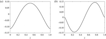
cannot be determined solely from the outer solution: they are obtained from our boundary layer analysis and are each plotted in figure 10. We show in the previous section that
 $\overline{p}_{11}$
and
 $\overline{w}_{01}$
both scale with
 $1/K$
, thus the stress also scales with
 $1/K$
at
 $O({\it\epsilon})$
.
The interfacial stress predicted by the inner flows (from (2.60)) at
 $O({\it\epsilon})$
. (a) The normal stress (we plot
 $K\overline{p}_{11}(0,z)$
) and (b) the shear stress (we plot
 $6z(1-z)K\overline{w}_{01}(0,z)$
). As both the normal and shear stress scale with
 $1/K$
at this order, both plotted terms are independent of
 $K$
.

Additionally, since we have imposed
 $P(0,z)=0$
, we have no
 $O({\it\epsilon}/{\it\delta})$
constant term from the pressure in the normal stress (2.60a
). In three dimensions, the tangential (that is, in the
 $(\boldsymbol{e}_{x}\times \boldsymbol{e}_{z})$
-direction) variation in pressure ensures that there will be an
 $O({\it\epsilon}/{\it\delta})$
term in the corresponding normal stress component no matter how we define the pressure (as we show in § 3.6.1).
We have now solved for the flow variables within the inflow boundary layers for the regions that affect the stress and the pressure drop. As shown in figure 7, there are further boundary layers which are important for inflow, and we discuss these in appendix A.
2.5.4 Summary
The main part of the leading-order inflow may be summarized as follows. The leading-order axial flow and pressure are unchanged until they reach the interface, after which they transition to plug flow inside the obstacle in region III, whose length is comparable to the channel height. This has an effect on the correction to normal flow and pressure in region II. Meanwhile, the tangential velocity satisfies the no tangential slip condition on the obstacle surface in region IIa – a boundary layer of even smaller width, which is comparable to the length of the channel height multiplied by the reciprocal of the Reynolds number.
Combining the original asymptotic expansion (2.26) with the asymptotic expansion in region II, namely (2.36c
), we deduce that the pressure jump between outer inflow regions I and IV is
 $O({\it\epsilon})$
. Specifically, we have determined that
 $$\begin{eqnarray}\displaystyle {\it\Pi}^{-}\sim \frac{{\it\alpha}}{K}\quad \text{as }{\it\epsilon},{\it\delta}\rightarrow 0~\text{with }{\it\epsilon}\ll {\it\delta}\ll 1, & & \displaystyle\end{eqnarray}$$
where
 ${\it\alpha}\approx -0.117$
.
The argument presented in this section will not hold if the fluid is leaving the obstacle rather than entering it. This is because the boundary layer region IIa is only valid for inflow (as can be seen from (2.55)). We reconsider our approach for outflow in the next section.
2.5.5 Outflow
The outflow inner problem (within regions V and VI) is shown in figure 5. We again seek a solution as
 ${\it\delta}\rightarrow 0$
with
 ${\it\epsilon}\ll {\it\delta}\ll 1$
using the method of matched asymptotic expansions.
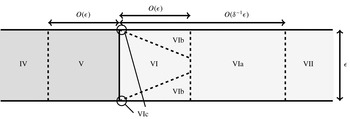
The asymptotic structure for outflow is shown schematically in figure 11. The flow in region V is unchanged at leading order and reaches the interface as uniform plug flow with magnitude
 $1$
. There is an inviscid core in the centre of region VI, flanked by Prandtl boundary layers near
 $z=0,1$
whose thicknesses are of
 $O(({\it\delta}X^{+})^{1/2})$
. These boundary layers (region VIb) grow downstream, and the transition to Poiseuille flow occurs when their thicknesses become of
 $O(1)$
. This occurs on a horizontal length scale of
 $O(1/{\it\delta})$
in a transition region we denote region VIa. There is a third boundary layer, denoted region VIc, which occurs in the corner between the channel wall and the porous interface. This region deals with a singularity at the corner that arises in region VIb, as in the classic Prandtl problem.
Schematic diagram of the inner regions for outflow – VIa, VIb, and VIc. The size of the boundary region VIb has been exaggerated for illustrative purposes, is of height
 $O({\it\epsilon}{\it\delta}^{1/2})$
, and grows proportional to the square root of the distance from the porous obstacle. Region VIc lies within region VIb and has height and length
 $O({\it\epsilon}{\it\delta})$
.

In this section, we investigate the regions VI and VIa to understand the transition from plug to Poiseuille flow and to calculate the pressure jump between the outer regions IV and VII. Regions VIb and VIc are discussed in appendix B.1 since they are not important to the transition. Recall that, from (2.61), we calculated an
 $O({\it\epsilon})$
pressure jump between outer regions I and IV for inflow. We show that the pressure jump between outer regions IV and VII is of
 $O({\it\epsilon}/{\it\delta})$
for outflow.
We start by investigating how the fluid moves through region VI. The leading-order behaviour is plug flow, and we determine the effect of the interfacial no tangential slip condition on the correction to the plug flow. In particular, we determine the far-field behaviour of the flow, which allows us to impose the correct matching conditions for the problem of transition to Poiseuille flow in region VIa.
2.5.6 Inner regions V and VI
To determine the outflow pressure jump (2.35b ), we must consider first-order flow terms. Therefore, we pose the asymptotic expansions
 $$\begin{eqnarray}\overline{\boldsymbol{u}}_{0}\sim \boldsymbol{e}_{x}+{\it\delta}^{1/2}\overline{\boldsymbol{u}}_{0a},\quad \overline{\boldsymbol{Q}}_{0}\sim \boldsymbol{e}_{x}+{\it\delta}^{1/2}\overline{\boldsymbol{Q}}_{0a},\quad \overline{p}_{1}\sim {\it\delta}^{-1/2}\overline{p}_{1a},\quad \overline{P}_{1}\sim -\frac{X^{+}}{K}+{\it\delta}^{1/2}\overline{P}_{1b},\end{eqnarray}$$
as
 ${\it\delta}\rightarrow 0$
, where the non-integer powers of
 ${\it\delta}$
arise due to the correction terms from the boundary layers in region VIb near the channel walls. We determine the leading-order behaviour within the coupled regions V and VI, but do not fully solve for the higher-order terms due to their complexity. Instead, we analyse the higher-order problems to obtain the information required for the matching condition with the transition region VIa.
Substituting the asymptotic expansions (2.62) into the system outlined in figure 5, the leading-order equations are trivially satisfied. The
 $O({\it\delta}^{1/2})$
exterior flow equations are
 $$\begin{eqnarray}\overline{u}_{0aX^{+}}=-\overline{p}_{1aX^{+}},\quad \overline{w}_{0aX^{+}}=-\overline{p}_{1az},\quad 0=\overline{u}_{0aX^{+}}+\overline{w}_{0az}\quad \text{in region VI},\end{eqnarray}$$
and the
 $O({\it\delta}^{1/2})$
interior flow equations are
 $$\begin{eqnarray}\overline{\boldsymbol{Q}}_{0a}=-K\boldsymbol{{\rm\nabla}}\overline{P}_{1b},\quad 0=\boldsymbol{{\rm\nabla}}\boldsymbol{\cdot }\overline{\boldsymbol{Q}}_{0a}\quad \text{in region V}.\end{eqnarray}$$
In region V, the first correction to the boundary condition on the channel walls is given by
 $$\begin{eqnarray}\displaystyle \overline{W}_{0a}=0\quad \text{on }z=0,1\text{ for }X^{+}<0, & & \displaystyle\end{eqnarray}$$
while the far-field conditions are obtained by matching with region IV, to yield
 $$\begin{eqnarray}\overline{P}_{1b}\rightarrow 0,\quad \overline{\boldsymbol{Q}}_{0a}\rightarrow \mathbf{0}\quad \text{as }X^{+}\rightarrow -\infty ~\text{for }0<z<1.\end{eqnarray}$$
In region VI, the boundary conditions on the channel walls are obtained by matching with region VIb. We show in appendix B.1 that, at this order, the flow problem within region VIb is equivalent to the standard Prandtl problem of uniform flow past a flat plate (Prandtl Reference Prandtl and Krazer1905). The matching conditions are therefore given by
 $$\begin{eqnarray}\displaystyle & \displaystyle \overline{w}_{0a}=\tilde{{\it\beta}}(4X^{+})^{-1/2}\quad \text{on }z=0\text{ for }X^{+}>0, & \displaystyle\end{eqnarray}$$
 $$\begin{eqnarray}\displaystyle & \displaystyle \overline{w}_{0a}=-\tilde{{\it\beta}}(4X^{+})^{-1/2}\quad \text{on }z=1\text{ for }X^{+}>0, & \displaystyle\end{eqnarray}$$
 $\tilde{{\it\beta}}$
(
 ${\approx}\,$
1.721) is a constant that is determined numerically from a nonlinear ordinary differential equation (discussed further in appendix B.1); the parameter
 ${\it\beta}$
used in Van Dyke (Reference Van Dyke1970) and Wilson (Reference Wilson1971) is related to
 $\tilde{{\it\beta}}$
via
 $\tilde{{\it\beta}}=2^{1/2}{\it\beta}$
. Finally, the interfacial conditions on
 $X^{+}=0$
are
 $$\begin{eqnarray}\overline{u}_{0a}=\overline{U}_{0a},\quad \overline{p}_{1a}=0,\quad \overline{w}_{0a}=0\quad \text{on }X^{+}=0\text{ for }0<z<1.\end{eqnarray}$$
We do not solve the coupled system of equations (2.64)–(2.68) here, though we note that it is possible to obtain an implicit representation for
 $\overline{w}_{0a}$
via a Fourier transformation. Instead, we acquire the necessary information for the matching with region VIa, which allows us to determine
 ${\it\Pi}_{0}^{+}$
in the next section. We note that (2.63) can be rearranged to deduce the following three results: firstly, that
 $$\begin{eqnarray}\displaystyle {\rm\nabla}^{2}\overline{w}_{0a}=0\quad \text{in region VI}; & & \displaystyle\end{eqnarray}$$
secondly, that
 $\overline{p}_{1a}$
is the harmonic conjugate of
 $\overline{w}_{0a}$
; and, thirdly, that
 $\overline{p}_{1a}+\overline{u}_{1a}$
is independent of
 $X^{+}$
. We deduce the leading-order far-field behaviour of
 $\overline{w}_{0a}$
by considering the governing equation (2.69) together with the channel wall boundary conditions (2.67) as
 $X^{+}\rightarrow \infty$
, to obtain the expansion
 $$\begin{eqnarray}\displaystyle \overline{w}_{0a}\sim \frac{\tilde{{\it\beta}}(1-2z)}{(4X^{+})^{1/2}}\quad \text{as }X^{+}\rightarrow \infty ~\text{for }0<z<1. & & \displaystyle\end{eqnarray}$$
Using the far-field condition (2.70) in the governing equations (2.63a,c ), we further deduce that
 $$\begin{eqnarray}\overline{u}_{0a}\sim \tilde{{\it\beta}}(4X^{+})^{1/2},\quad \overline{p}_{1a}\sim -\tilde{{\it\beta}}(4X^{+})^{1/2}\quad \text{as }X^{+}\rightarrow \infty ~\text{for }0<z<1.\end{eqnarray}$$
We note that the far-field expansions (2.70)–(2.71) have no dependence on the permeability
 $K$
. As these far-field expansions are used to form matching conditions, which transfer information into the transition region VIa (which is where we calculate the pressure drop
 ${\it\Pi}_{0}^{+}$
), we note that
 ${\it\Pi}_{0}^{+}$
will be independent of
 $K$
. We carry out this matching in appendix B.2.
The components of stress on the interface at
 $x=1$
are given by
 $$\begin{eqnarray}\displaystyle & \displaystyle {\it\sigma}_{xx}=-\hspace{-3.0pt}\left(12-\frac{2}{K}+{\it\epsilon}{\it\delta}^{-1/2}\overline{p}_{1a}\right)+\mathit{o}({\it\epsilon}{\it\delta}^{-1/2}), & \displaystyle\end{eqnarray}$$
 $$\begin{eqnarray}\displaystyle & \displaystyle {\it\sigma}_{xz}={\it\epsilon}{\it\delta}^{1/2}\left(\overline{u}_{0az}+\overline{w}_{0aX^{+}}\right)+\mathit{o}({\it\epsilon}{\it\delta}^{1/2}) & \displaystyle\end{eqnarray}$$
 ${\it\epsilon},{\it\delta}\rightarrow 0$
with
 ${\it\epsilon}\ll {\it\delta}\ll 1$
, where we have not explicitly calculated
 $\overline{p}_{1a}$
,
 $\overline{u}_{0a}$
, or
 $\overline{w}_{0a}$
. In terms of the first order at which the stress varies in
 $z$
, we find that the normal stress (2.72a
) for outflow is a factor of
 $O({\it\delta}^{-1/2})$
larger than for inflow (2.60a
), while the shear stress (2.72b
) for outflow is a factor of
 $O({\it\delta}^{1/2})$
smaller than for inflow (2.60b
).
2.5.7 Transition region VIa
We now consider the region in which the flow transitions from plug to Poiseuille flow. This occurs when the growing Prandtl boundary layers with thickness of
 $O(({\it\delta}X^{+})^{1/2})$
become of
 $O(1)$
, that is, when
 $X^{+}=O(1/{\it\delta})$
, bringing about a balance in the exterior flow equations between fluid momentum and viscosity across the full channel width. Recall that we have called this region VIa, as illustrated in figure 11.
The relevant scalings are
 $X^{+}={\it\delta}^{-1}\widetilde{X}$
and
 $\overline{w}_{0}={\it\delta}\widetilde{w}_{0}$
, and we introduce the new variables
 $\overline{u}_{0}=\widetilde{u}_{0}$
and
 $\overline{p}_{1}=\widetilde{p}_{1}$
to signify that we are working in region VIa. Then, in region VIa (where
 $0<\widetilde{X}<\infty$
and
 $0<z<1$
) the exterior flow equations given in figure 5 become
 $$\begin{eqnarray}\displaystyle & \displaystyle \widetilde{u}_{0}\widetilde{u}_{0\widetilde{X}}+\widetilde{w}_{0}\widetilde{u}_{0z}=-{\it\delta}\widetilde{p}_{1\widetilde{X}}+{\it\delta}^{2}\widetilde{u}_{0\widetilde{X}\widetilde{X}}+\widetilde{u}_{0zz}, & \displaystyle\end{eqnarray}$$
 $$\begin{eqnarray}\displaystyle & \displaystyle {\it\delta}^{2}(\widetilde{u}_{0}\widetilde{u}_{0\widetilde{X}}+\widetilde{w}_{0}\widetilde{w}_{0z})=-{\it\delta}\widetilde{p}_{1z}+{\it\delta}^{4}\widetilde{w}_{0\widetilde{X}\widetilde{X}}+{\it\delta}^{2}\widetilde{w}_{0zz}, & \displaystyle\end{eqnarray}$$
 $$\begin{eqnarray}\displaystyle & \displaystyle \widetilde{u}_{0\widetilde{X}}+\widetilde{w}_{0z}=0. & \displaystyle\end{eqnarray}$$
We pose the asymptotic expansions
 $$\begin{eqnarray}\widetilde{u}_{0}=\widetilde{u}_{00}+O({\it\delta}^{1/2}),\quad \widetilde{w}_{0}=\widetilde{w}_{01}+O({\it\delta}^{1/2}),\quad \widetilde{p}_{1}={\it\delta}^{-1}\widetilde{p}_{10}+O({\it\delta}^{-1/2}),\end{eqnarray}$$
as
 ${\it\delta}\rightarrow 0$
, and substitute them into the governing equations (2.73) to yield the following leading-order governing equations in region VIa:
 $$\begin{eqnarray}\widetilde{u}_{00}\widetilde{u}_{00\widetilde{X}}+\widetilde{w}_{01}\widetilde{u}_{00z}=-\widetilde{p}_{10\widetilde{X}}+\widetilde{u}_{00zz},\quad 0=-\widetilde{p}_{10z},\quad \widetilde{u}_{00\widetilde{X}}+\widetilde{w}_{01z}=0.\end{eqnarray}$$
The boundary conditions on the channel walls become
 $$\begin{eqnarray}\displaystyle \overline{\boldsymbol{u}}_{00}=\mathbf{0}\quad \text{on }z=0,1\text{ for}~\widetilde{X}>0. & & \displaystyle\end{eqnarray}$$
The leading-order matching conditions are derived in appendix B.2. They are obtained by forming composite expansions between regions VI and VIb, then using Van Dyke’s matching rule (Van Dyke Reference Van Dyke1975). We use the multiplicative composite expansions (Van Dyke Reference Van Dyke1975) to ensure that the matching condition for the velocity satisfies the no-slip condition on the channel walls. This allows a greater accuracy when we solve numerically the resulting system. The matching conditions are given by
 $$\begin{eqnarray}\displaystyle & \displaystyle \widetilde{u}_{00}\sim (1+2\tilde{{\it\beta}}\widetilde{X}^{1/2})f^{\prime }(\widetilde{{\it\eta}}_{(0)})f^{\prime }(\widetilde{{\it\eta}}_{(1)}), & \displaystyle\end{eqnarray}$$
 $$\begin{eqnarray}\displaystyle & \displaystyle \widetilde{w}_{01}\sim \frac{(1-2z)}{2\tilde{{\it\beta}}\widetilde{X}^{1/2}}(\widetilde{{\it\eta}}_{(0)}f^{\prime }(\widetilde{{\it\eta}}_{(0)})-f(\widetilde{{\it\eta}}_{(0)}))(f(\widetilde{{\it\eta}}_{(1)})-\widetilde{{\it\eta}}_{(1)}f^{\prime }(\widetilde{{\it\eta}}_{(1)})), & \displaystyle\end{eqnarray}$$
 $$\begin{eqnarray}\displaystyle & \displaystyle \widetilde{p}_{10}\sim -2\tilde{{\it\beta}}\widetilde{X}^{1/2}, & \displaystyle\end{eqnarray}$$
 $\widetilde{X}\downarrow 0$
, where
 $f$
is the standard Blasius similarity solution (defined in (B 7)),
 $\widetilde{{\it\eta}}_{(0)}=z/\widetilde{X}^{1/2}$
and
 $\widetilde{{\it\eta}}_{(1)}=(1-z)/\widetilde{X}^{1/2}$
. The matching conditions (2.77) are consistent with a small
 $\widetilde{X}$
expansion (for fixed
 $z$
) of the governing equations (2.75). The matching conditions between regions VIa and VII are given by
 $$\begin{eqnarray}\widetilde{u}_{00}\sim 6z(1-z),\quad \widetilde{w}_{01}\rightarrow 0,\quad \widetilde{p}_{10}\sim -12\widetilde{X}+{\it\Pi}_{0}^{+}\quad \text{as}~\widetilde{X}\rightarrow \infty ~\text{for }0<z<1,\end{eqnarray}$$
where
 ${\it\Pi}_{0}^{+}$
is determined from the solution in region VIa. The full system for the flow in region VIa is given by (2.75)–(2.78).
In Bodoia & Osterle (Reference Bodoia and Osterle1961), this same transition region was considered, though was not derived formally through asymptotic methods. The authors used the boundary conditions
 $$\begin{eqnarray}\widetilde{u}_{00}=1,\quad \widetilde{w}_{01}=0,\quad \widetilde{p}_{10}=0\quad \text{on}~\widetilde{X}=0\text{ for }0<z<1,\end{eqnarray}$$
instead of the matching conditions (2.77). We note that, unlike (2.77b
), the condition (2.79b
) is not consistent with the small
 $\widetilde{X}$
approximation to the governing equations (2.75), from which it can be deduced that
 $\widetilde{w}_{01}$
is singular at the corners at
 $\widetilde{X}=0$
,
 $z=0,1$
. With the boundary conditions (2.79), it was found in Bodoia & Osterle (Reference Bodoia and Osterle1961) that the pressure jump
 ${\it\Pi}_{0}^{+}\approx -0.338$
.
We now calculate
 ${\it\Pi}_{0}^{+}$
numerically using the formal matching conditions (2.77). We start the numerical simulation at
 $\widetilde{X}=10^{-4}$
to avoid the inverse square root singularities in
 $\widetilde{w}_{01}$
and in
 $\widetilde{p}_{10\widetilde{X}}$
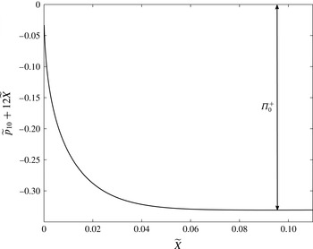
, and use the finite-difference scheme outlined in Bodoia & Osterle (Reference Bodoia and Osterle1961). In figure 12, we show the numerical solutions for
 $\widetilde{p}_{10}+12\widetilde{X}$
as a function of
 $\widetilde{X}$
, and we emphasise that
 $\widetilde{p}_{10}$
is independent of
 $z$
. From the matching condition (2.78c
), we determine that the value of the leading-order outflow pressure jump between outer regions IV and VII is given by
 ${\it\Pi}_{0}^{+}=-0.331$
to 3 significant figures. We note that the value of
 ${\it\Pi}^{+}$
found by Bodoia & Osterle (Reference Bodoia and Osterle1961) using their inconsistent boundary conditions (2.79) only differs by approximately 2 % from the value of
 ${\it\Pi}^{+}$
obtained using formal matching conditions.
Calculating the outflow pressure drop along the channel by plotting
 $\widetilde{p}_{10}+12\widetilde{X}$
. See text for further details.

Combining the original asymptotic expansion (2.26) with the asymptotic expansion in region VIa (2.74c
), we deduce that the pressure jump between outer outflow regions IV and VII is
 $O({\it\epsilon}/{\it\delta})$
. Specifically, we have determined that
 $$\begin{eqnarray}\displaystyle {\it\Pi}^{+}\sim \frac{{\it\Pi}_{0}^{+}}{{\it\delta}}\quad \text{as}~{\it\epsilon},{\it\delta}\rightarrow 0~\text{with}~{\it\epsilon}\ll {\it\delta}\ll 1, & & \displaystyle\end{eqnarray}$$
where
 ${\it\Pi}_{0}^{+}\approx -0.331$
.
2.6 Summary
We have thus far determined the boundary layer structure for two-dimensional flow through a channel with stationary walls containing a porous obstacle. We formulated the full problem for an
 $O(1)$
Reynolds number, then considered the asymptotic sublimits in which
 ${\it\epsilon}\ll Re\ll 1$
and
 $1\ll Re\ll 1/{\it\epsilon}$
. In the first sublimit, the inflow and outflow boundary layer structure was found to be the same, whereas in the latter sublimit, a rich boundary layer structure was unveiled, which differed for inflow and outflow. We determined how flow transitions from Poiseuille to plug for inflow and from plug back to Poiseuille for outflow, which allowed us to determine the leading-order asymptotic values of the pressure jumps
 ${\it\Pi}^{-}$
and
 ${\it\Pi}^{+}$
across regions II/III and regions V/VI, respectively. For inflow, where the flow problems in regions II and III decouple, we calculated the stress acting on the interface up to the order at which there is a variation in
 $z$
. For outflow, where the relevant flow problems in regions V and VI are coupled, we determined the scalings of the stress acting on the interface up to the order at which there is a variation in
 $z$
.
In the next section, we generalize the problem and consider unsteady three-dimensional flow in a Hele-Shaw cell past a tight-fitting, highly permeable cylindrical porous obstacle, with a smooth boundary. As the fluid can now travel around the porous obstacle, the high Reynolds number limit has an entrainment effect for outflow. We show that this entrainment can lead to a net force acting on the obstacle, even when the unidirectional far-field forcing is periodic with a zero mean.
3 Unsteady three-dimensional flow
A schematic of the three-dimensional problem is illustrated in figure 2(b), and a two-dimensional plan view is illustrated in figure 13. We initially work in a Cartesian coordinate system
 $(x,y,z)$
with origin at the obstacle centre of mass projected onto the planar plate of the Hele-Shaw cell in the plane
 $z=0$
, the other plate lying in the plane
 $z=h$
. The obstacle axis is normal to the two parallel flat sides of the Hele-Shaw cell, and is parallel to the
 $z$
-axis. The typical cross-sectional extent of the obstacle is
 $l$
, the Hele-Shaw cell height is
 $h$
, and we shall also assume that
 ${\it\epsilon}=h/l\ll 1$
.
Plan view of streamlines through and around a general porous obstacle model with a uniform far-field flow. The
 $z$
-axis points out of the page. The Hele-Shaw cell has a depth of length
 $h$
in the
 $z$
-direction (not shown). We show the unit vectors
 $\boldsymbol{e}_{x}$
and
 $\boldsymbol{e}_{y}$
in the
 $x$
- and
 $y$
-directions respectively (for the Cartesian coordinate system), and the curvilinear
 $(n,s)$
-coordinate system for a given point on the boundary of the obstacle.

The exterior and interior fluid velocities are denoted by
 $\boldsymbol{u}^{s}=u^{s}\boldsymbol{e}_{x}+v^{s}\boldsymbol{e}_{y}+w^{s}\boldsymbol{e}_{z}$
and
 $\boldsymbol{Q}^{s}=U^{s}\boldsymbol{e}_{x}+V^{s}\boldsymbol{e}_{y}+W^{s}\boldsymbol{e}_{z}$
, respectively. The exterior and interior fluid pressures are denoted by
 $p^{s}$
and
 $P^{s}$
, respectively. We use the superscript
 $s$
to denote variables in the three-dimensional problem, and we later reduce the three-dimensional problem by relating these variables to their two-dimensional counterparts in the three-dimensional analogue of the inner regions considered in §§ 2.3–2.5. The typical magnitude of the unidirectional far-field flow is
 $U_{\infty }$
. We non-dimensionalize by scaling the variables as follows:
 $(x,y)\sim l$
,
 $z\sim {\it\epsilon}l$
,
 $t\sim l/U_{\infty }$
(corresponding to an
 $O(1)$
Strouhal number),
 $(p^{s},P^{s})\sim {\it\mu}U_{\infty }/({\it\epsilon}h)$
,
 $(u^{s},v^{s},U^{s},V^{s})\sim U_{\infty }$
and
 $(w^{s},W^{s})\sim {\it\epsilon}U_{\infty }$
. With these scalings, the dimensionless Navier–Stokes equations, which hold inside the Hele-Shaw cell but outside the porous obstacle, are given by
 $$\begin{eqnarray}\displaystyle & \displaystyle {\it\epsilon}\overline{Re}(u_{t}^{s}+\boldsymbol{u}^{s}\boldsymbol{\cdot }\boldsymbol{{\rm\nabla}}u^{s})=-p_{x}^{s}+{\it\epsilon}^{2}{\rm\nabla}_{\bot }^{2}u^{s}+u_{zz}^{s}, & \displaystyle\end{eqnarray}$$
 $$\begin{eqnarray}\displaystyle & \displaystyle {\it\epsilon}\overline{Re}(v_{t}^{s}+\boldsymbol{u}^{s}\boldsymbol{\cdot }\boldsymbol{{\rm\nabla}}v^{s})=-p_{y}^{s}+{\it\epsilon}^{2}{\rm\nabla}_{\bot }^{2}v^{s}+v_{zz}^{s}, & \displaystyle\end{eqnarray}$$
 $$\begin{eqnarray}\displaystyle & \displaystyle {\it\epsilon}^{3}\overline{Re}(w_{t}^{s}+\boldsymbol{u}^{s}\boldsymbol{\cdot }\boldsymbol{{\rm\nabla}}w^{s})=-p_{z}^{s}+{\it\epsilon}^{4}{\rm\nabla}_{\bot }^{2}w^{s}+{\it\epsilon}^{2}w_{zz}^{s}, & \displaystyle\end{eqnarray}$$
 $$\begin{eqnarray}\displaystyle & \displaystyle 0=\boldsymbol{{\rm\nabla}}\boldsymbol{\cdot }\boldsymbol{u}^{s}, & \displaystyle\end{eqnarray}$$
 $\overline{Re}={\it\rho}hU_{\infty }/{\it\mu}$
is the global Reynolds number,
 $\boldsymbol{{\rm\nabla}}$
is the three-dimensional gradient operator and
 ${\rm\nabla}_{\bot }^{2}=\partial _{xx}+\partial _{yy}$
is the two-dimensional Laplacian operator. The dimensionless Darcy equations, which hold inside the porous obstacle, are given by
 $$\begin{eqnarray}U^{s}=-KP_{x}^{s},\quad V^{s}=-KP_{y}^{s},\quad {\it\epsilon}^{2}W^{s}=-KP_{z}^{s},\quad 0=\boldsymbol{{\rm\nabla}}\boldsymbol{\cdot }\boldsymbol{Q}^{s},\end{eqnarray}$$
where
 $K=k/h^{2}\ll 1$
, as before.
3.1 Boundary conditions
The boundary conditions on the plates of the Hele-Shaw cell at
 $z=0$
,
 $1$
are those of no slip and no flux for the exterior flow and of no flux for the interior flow, so that
 $$\begin{eqnarray}\displaystyle & \displaystyle \boldsymbol{u}^{s}=\mathbf{0}\quad \text{on }z=0,1\quad \text{outside the obstacle}, & \displaystyle\end{eqnarray}$$
 $$\begin{eqnarray}\displaystyle & \displaystyle W^{s}=0\quad \text{on }z=0,1\quad \text{inside the obstacle}. & \displaystyle\end{eqnarray}$$
On the interface, we impose three-dimensional equivalents of the two-dimensional interfacial conditions given by (2.4). These are continuity of normal flux, continuity of pressure and a no tangential slip condition, as follows
 $$\begin{eqnarray}\displaystyle & \displaystyle \boldsymbol{u}^{s}\boldsymbol{\cdot }\boldsymbol{n}=\boldsymbol{Q}^{s}\boldsymbol{\cdot }\boldsymbol{n}, & \displaystyle\end{eqnarray}$$
 $$\begin{eqnarray}\displaystyle & \displaystyle p^{s}=P^{s}, & \displaystyle\end{eqnarray}$$
 $$\begin{eqnarray}\displaystyle & \displaystyle \boldsymbol{u}^{s}-(\boldsymbol{u}^{s}\boldsymbol{\cdot }\boldsymbol{n})\boldsymbol{n}=\mathbf{0}, & \displaystyle\end{eqnarray}$$
 $\boldsymbol{n}$
is the unit normal pointing out of the porous obstacle.
The far-field condition is
 $$\begin{eqnarray}\displaystyle p^{s}\sim -12xG(t)\quad \text{as }x^{2}+y^{2}\rightarrow \infty , & & \displaystyle\end{eqnarray}$$
where
 $G(t)$
is a dimensionless function of time. We take
 $|G(t)|$
and
 $|G^{\prime }(t)|$
to be of
 $O(1)$
, so that the far-field forcing does not have a large velocity or acceleration.
3.2 Asymptotic structure
The dimensionless problem (3.1)–(3.5) is characterised by two length scales: the typical cross-sectional extent of the obstacle,
 $1$
, and the Hele-Shaw cell height,
 ${\it\epsilon}\ll 1$
. We again seek a solution using the method of matched asymptotic expansions in terms of the small parameter
 ${\it\epsilon}$
. We note that, in contrast to § 2, not all of the fluid has to pass through the porous obstacle as it is now able to flow around the porous obstacle. In this section, we show that this difference results in a Darcy velocity of
 $O(K)$
with an
 $O(1)$
pressure drop, in comparison to the two-dimensional case where the Darcy velocity was of
 $O(1)$
with an
 $O(1/K)$
pressure drop. As the continuity of flux condition (3.4a
) ensures that
 $\boldsymbol{u}^{s}\boldsymbol{\cdot }\boldsymbol{n}=O(K)$
near the interface, we are able to deduce that
 $K=O({\it\epsilon})$
corresponds to an obstacle which is impermeable at leading order in
 ${\it\epsilon}$
. As discussed previously, we wish to investigate the case where the obstacle is as permeable as possible, and we therefore consider the limit where
 ${\it\epsilon}\ll K\ll 1$
. The local Reynolds number (defined later) characterises the flow close to the interface. We initially consider the distinguished limit whereby the local Reynolds number is of
 $O(1)$
, then consider the asymptotic sublimits of a small and large local Reynolds number in more detail, as before.
The outer problems are characterised by an
 $O(1)$
length scale in the
 $(x,y)$
-plane (with the Hele-Shaw cell height,
 ${\it\epsilon}$
, being the length scale in the
 $z$
-direction), where we have at leading order Poiseuille and plug flow in the exterior and interior regions, respectively. We assume that the obstacle is a cylinder whose cross-section has a curvature of
 $O(1)$
, so that the surface near a point on the obstacle boundary is well approximated by the tangent plane at that point. The inner regions are then characterised by an
 $O({\it\epsilon})$
extension of each local normal plane to the interface and occur on either side of the interface, so that the inner problems are similar to those considered in § 2, and the boundary layer structure is its three-dimensional equivalent.
3.3 Outer regions
In the outer regions, we take asymptotic expansions in the limit as
 ${\it\epsilon}\rightarrow 0$
, of the form
 $$\begin{eqnarray}\displaystyle f=f_{0}+{\it\epsilon}f_{1}+O({\it\epsilon}^{2}), & & \displaystyle\end{eqnarray}$$
for
 $f\in \{u^{s},v^{s},w^{s},U^{s},V^{s},W^{s},p^{s},P^{s}\}$
. At leading-order we find that, exterior to the obstacle,
 $$\begin{eqnarray}u_{0}^{s}=g_{1}(z)p_{0x}^{s},\quad v_{0}^{s}=g_{1}(z)p_{0y}^{s},\quad w_{0}^{s}=0,\quad \boldsymbol{{\rm\nabla}}\boldsymbol{\cdot }\boldsymbol{u}_{0}^{s}=0,\end{eqnarray}$$
where
 $g_{1}(z)=z(z-1)/2$
, while interior to the obstacle,
 $$\begin{eqnarray}U_{0}^{s}=-KP_{0x}^{s},\quad V_{0}^{s}=-KP_{0y}^{s},\quad W_{0}^{s}=0,\quad \boldsymbol{{\rm\nabla}}\boldsymbol{\cdot }\boldsymbol{Q}_{0}^{s}=0,\end{eqnarray}$$
so that both the interior and exterior pressure satisfy Laplace’s equation in two dimensions. We define the two-dimensional cross-section of the obstacle as
 $D$
and the one-dimensional boundary of this as
 $\partial D$
. Thus, the governing equations are
 $$\begin{eqnarray}{\rm\nabla}_{\bot }^{2}p_{0}^{s}=0\quad \text{outside}~D,\quad {\rm\nabla}_{\bot }^{2}P_{0}^{s}=0\quad \text{in}~D.\end{eqnarray}$$
The far-field condition is
 $$\begin{eqnarray}\displaystyle p_{0}^{s}\sim -12xG(t)\quad \text{as }x^{2}+y^{2}\rightarrow \infty . & & \displaystyle\end{eqnarray}$$
In § 3.4, we find that the leading-order coupling conditions on the interface are
 $$\begin{eqnarray}p_{0}^{s}=P_{0}^{s},\quad \frac{\partial p_{0}^{s}}{\partial n}=12K\frac{\partial P_{0}^{s}}{\partial n}\quad \text{on}~\partial D,\end{eqnarray}$$
where (3.11b
) is equivalent to the continuity of total flux condition given in (2.11a
). The leading-order problem is defined by (3.9)–(3.11), and can be solved for a given obstacle boundary
 $\partial D$
. For future reference, we deduce from (3.8) that the segments of the boundary where we have inflow/outflow at leading order occur when
 $\partial P_{0}^{s}/\partial n$
evaluated on the boundary is positive/negative.
For the
 $O({\it\epsilon})$
correction terms we find that, outside
 $D$
,
 $$\begin{eqnarray}\displaystyle & \displaystyle u_{1}^{s}=\frac{\partial }{\partial x}\left(p_{1}^{s}g_{1}(z)+\overline{Re}\left(p_{0t}^{s}g_{2}(z)+|\boldsymbol{{\rm\nabla}}p_{0}^{s}|^{2}g_{3}(z)\right)\right), & \displaystyle\end{eqnarray}$$
 $$\begin{eqnarray}\displaystyle & \displaystyle v_{1}^{s}=\frac{\partial }{\partial y}\left(p_{1}^{s}g_{1}(z)+\overline{Re}\left(p_{0t}^{s}g_{2}(z)+|\boldsymbol{{\rm\nabla}}p_{0}^{s}|^{2}g_{3}(z)\right)\right), & \displaystyle\end{eqnarray}$$
 $$\begin{eqnarray}\displaystyle & \displaystyle w_{1}^{s}=-{\rm\nabla}_{\bot }^{2}\left(p_{1}^{s}\int _{0}^{z}g_{1}({\it\xi})\,\text{d}{\it\xi}+\overline{Re}|\boldsymbol{{\rm\nabla}}p_{0}^{s}|^{2}\int _{0}^{z}g_{3}({\it\xi})\,\text{d}{\it\xi}\right), & \displaystyle\end{eqnarray}$$
 $$\begin{eqnarray}\displaystyle & \displaystyle \boldsymbol{{\rm\nabla}}\boldsymbol{\cdot }\boldsymbol{u}_{1}^{s}=0, & \displaystyle\end{eqnarray}$$
where
 $$\begin{eqnarray}\displaystyle g_{2}(z)=\frac{g_{1}(z)}{12}(z^{2}-z+1), & & \displaystyle\end{eqnarray}$$
 $$\begin{eqnarray}\displaystyle g_{3}(z)=\frac{g_{1}(z)}{240}(2z^{4}-4z^{3}+z^{2}+z+1), & & \displaystyle\end{eqnarray}$$
while in the obstacle,
 $$\begin{eqnarray}U_{1}^{s}=-KP_{1x}^{s},\quad V_{1}^{s}=-KP_{1y}^{s},\quad W_{1}^{s}=0,\quad \boldsymbol{{\rm\nabla}}\boldsymbol{\cdot }\boldsymbol{Q}_{1}^{s}=0\quad \text{in}~D,\end{eqnarray}$$
so that the pressures satisfy
 $$\begin{eqnarray}{\rm\nabla}_{\bot }^{2}\left(p_{1}^{s}+\frac{3\overline{Re}}{560}|\boldsymbol{{\rm\nabla}}p_{0}^{s}|^{2}\right)=0\quad \text{outside}~D,\quad {\rm\nabla}_{\bot }^{2}P_{1}^{s}=0\quad \text{in}~D.\end{eqnarray}$$
The time derivative of
 ${\rm\nabla}^{2}p_{0}^{s}$
does not appear in (3.14a
) due to the governing equation (3.9a
). The far-field condition is
 $$\begin{eqnarray}\displaystyle p_{1}^{s}\rightarrow 0\quad \text{as }x^{2}+y^{2}\rightarrow \infty . & & \displaystyle\end{eqnarray}$$
The first-order coupling conditions on the interface are determined in § 3.4 and appendix C, and are given by
 $$\begin{eqnarray}\displaystyle & \displaystyle p_{1}^{s}-P_{1}^{s}={\it\Pi}^{s-}H(-\boldsymbol{u}_{0}\boldsymbol{\cdot }\boldsymbol{n})+{\it\Pi}^{s+}H(\boldsymbol{u}_{0}\boldsymbol{\cdot }\boldsymbol{n}), & \displaystyle\end{eqnarray}$$
 $$\begin{eqnarray}\displaystyle & \displaystyle \frac{\partial }{\partial n}\left(p_{1}^{s}-\frac{\overline{Re}}{10}\left(p_{0t}^{s}-\frac{3}{56}|\boldsymbol{{\rm\nabla}}p_{0}^{s}|^{2}\right)\right)-12K\frac{\partial P_{1}^{s}}{\partial n}={\it\Lambda}^{s-}H(-\boldsymbol{u}_{0}\boldsymbol{\cdot }\boldsymbol{n})+{\it\Lambda}^{s+}H(\boldsymbol{u}_{0}\boldsymbol{\cdot }\boldsymbol{n}), & \displaystyle \nonumber\\ \displaystyle & & \displaystyle\end{eqnarray}$$
 $\boldsymbol{u}_{0}\boldsymbol{\cdot }\boldsymbol{n}\neq 0$
, where a superscript ending in
 $-/+$
refers to an inflow/outflow quantity, and
 $H(x)$
is the Heaviside step function. These inflow/outflow segments of
 $\partial D$
are determined from (3.7)–(3.11) as previously discussed. The presence of the Heaviside functions in (3.16) introduces the possibility of pressure singularities appearing at points on the boundary at which
 $\boldsymbol{u}_{0}\boldsymbol{\cdot }\boldsymbol{n}=0$
. We discuss this in more detail once we determine the asymptotic approximations of the coefficients premultiplying these functions.
The coupling condition (3.16b
) represents conservation of mass across the interface at this order and, in contrast to the two-dimensional versions (2.19a
), (2.20a
), has additional terms which correspond to an entrainment effect at this order. That is, the jump in the
 $O({\it\epsilon})$
average normal velocity across the interface (between outer regions) has a contribution from the variation of the leading-order tangential velocity in the inner regions.
3.4 Inner regions
As the inner regions are close to the obstacle boundary, it will be convenient to work in general curvilinear coordinates
 $(n,s,z)$
such that
 $n=0$
on the boundary, with
 $n>0$
corresponding to the exterior of
 $D$
, and
 $s$
being the arc length along the boundary measured anticlockwise, as illustrated in figure 13.
The relevant inner scalings are
 $n={\it\epsilon}N$
and
 $(w^{s},W^{s})=(\overline{w}^{s},\overline{W}^{s})/{\it\epsilon}$
, and we define the components of fluid velocity in curvilinear coordinates by
 $\overline{\boldsymbol{u}}^{s}=\overline{u}^{s}\boldsymbol{n}+\overline{v}^{s}\boldsymbol{t}+\overline{w}^{s}\boldsymbol{e}_{z}$
and
 $\overline{\boldsymbol{Q}}^{s}=\overline{U}^{s}\boldsymbol{n}+\overline{V}^{s}\boldsymbol{t}+\overline{W}^{s}\boldsymbol{e}_{z}$
in the exterior and interior regions, respectively. Under these scalings, the exterior flow equations (3.1) become (see, for example, Schlichting & Gersten (Reference Schlichting and Gersten2000))
 $$\begin{eqnarray}\displaystyle & \displaystyle \overline{Re}(\overline{u}^{s}\overline{u}_{N}^{s}+\overline{w}^{s}\overline{u}_{z}^{s})+O({\it\epsilon}\overline{Re})=-{\it\epsilon}^{-1}\overline{p}_{N}^{s}+\overline{u}_{NN}^{s}+\overline{u}_{zz}^{s}+O({\it\epsilon}), & \displaystyle\end{eqnarray}$$
 $$\begin{eqnarray}\displaystyle & \displaystyle \overline{Re}(\overline{u}^{s}\overline{v}_{N}^{s}+\overline{w}^{s}\overline{v}_{z}^{s})+O({\it\epsilon}\overline{Re})=-\overline{p}_{s}^{s}+\overline{v}_{NN}^{s}+\overline{v}_{zz}^{s}+O({\it\epsilon}), & \displaystyle\end{eqnarray}$$
 $$\begin{eqnarray}\displaystyle & \displaystyle \overline{Re}(\overline{u}^{s}\overline{w}_{N}^{s}+\overline{w}^{s}\overline{w}_{z}^{s})+O({\it\epsilon}\overline{Re})=-{\it\epsilon}^{-1}\overline{p}_{z}^{s}+\overline{w}_{NN}^{s}+\overline{w}_{zz}^{s}+O({\it\epsilon}), & \displaystyle\end{eqnarray}$$
 $$\begin{eqnarray}\displaystyle & \displaystyle 0=\overline{u}_{N}^{s}+\overline{w}_{z}^{s}+{\it\epsilon}({\it\kappa}(s)\overline{u}^{s}+\overline{v}_{s}^{s})+O({\it\epsilon}^{2}), & \displaystyle\end{eqnarray}$$
 ${\it\kappa}(s)$
denotes the curvature of the obstacle boundary (positive if the centre of the osculating circle lies in the region in which
 $n<0$
for a given
 $s$
), and we assume that
 $|{\it\kappa}|=O(1)$
. Similarly, the interior flow equations (3.2) become
 $$\begin{eqnarray}\displaystyle & \displaystyle {\it\epsilon}\overline{U}^{s}=-K\overline{P}_{N}^{s}, & \displaystyle\end{eqnarray}$$
 $$\begin{eqnarray}\displaystyle & \displaystyle \overline{V}^{s}=-K\overline{P}_{s}^{s}+O({\it\epsilon}), & \displaystyle\end{eqnarray}$$
 $$\begin{eqnarray}\displaystyle & \displaystyle {\it\epsilon}\overline{W}^{s}=-K\overline{P}_{z}^{s}, & \displaystyle\end{eqnarray}$$
 $$\begin{eqnarray}\displaystyle & \displaystyle 0=\overline{U}_{N}^{s}+\overline{W}_{z}^{s}+{\it\epsilon}({\it\kappa}(s)\overline{U}^{s}+\overline{V}_{s}^{s})+O({\it\epsilon}^{2}). & \displaystyle\end{eqnarray}$$
 $$\begin{eqnarray}\displaystyle & \displaystyle \overline{\boldsymbol{u}}^{s}=\mathbf{0}\quad \text{on }z=0,1\text{ for}~N>0, & \displaystyle\end{eqnarray}$$
 $$\begin{eqnarray}\displaystyle & \displaystyle \overline{W}^{s}=0\quad \text{on }z=0,1\text{ for}~N<0. & \displaystyle\end{eqnarray}$$
 $N=0$
become
 $$\begin{eqnarray}\overline{u}^{s}=\overline{U}^{s},\quad \overline{p}^{s}=\overline{P}^{s},\quad \overline{v}^{s}=0,\quad \overline{w}^{s}=0.\end{eqnarray}$$
We form inner expansions in powers of
 ${\it\epsilon}$
as follows:
 $$\begin{eqnarray}\displaystyle (\overline{\boldsymbol{u}}^{s},\overline{\boldsymbol{Q}}^{s},\overline{p}^{s},\overline{P}^{s})=(\overline{\boldsymbol{u}}_{0}^{s},\overline{\boldsymbol{Q}}_{0}^{s},\overline{p}_{0}^{s},\overline{P}_{0}^{s})+{\it\epsilon}(\overline{\boldsymbol{u}}_{1}^{s},\overline{\boldsymbol{Q}}_{1}^{s},\overline{p}_{1}^{s},\overline{P}_{1}^{s})+O({\it\epsilon}^{2})\quad \text{as}~{\it\epsilon}\rightarrow 0;\quad & & \displaystyle\end{eqnarray}$$
substituting these expansions into the inner exterior flow equations (3.17a,c
) and the interior flow equations (3.18a,c
), then equating powers of
 ${\it\epsilon}$
, yields the leading-order pressure equations
 $$\begin{eqnarray}0=-\overline{p}_{0N}^{s},\quad 0=-\overline{p}_{0z}^{s},\quad 0=-\overline{P}_{0N}^{s},\quad 0=-\overline{P}_{0z}^{s}.\end{eqnarray}$$
This leading-order system is the same as in the two-dimensional case, and we proceed in exactly the same way. Matching with the outer pressures, and using the leading-order version of the continuity of pressure condition (3.20b ), we deduce that the leading-order pressures are unchanged through the inner regions and we are justified in writing the coupling condition (3.11a ). In a similar manner, integrating the leading-order version of the continuity equations (3.17d ) and (3.18d ) over the cell height, using the cell wall boundary conditions (3.19), and then matching with the outer regions, justifies the coupling condition (3.11b ). The entrainment effect does not occur at this order.
The first-order flow equations in the
 $(N,z)$
-plane decouple from the tangential velocities
 $\overline{v}^{s}$
and
 $\overline{V}^{s}$
, and the tangential coordinate
 $s$
can be treated as a parameter in the problem. We can further reduce these problems to the two-dimensional cases considered previously using the scalings
 $$\begin{eqnarray}\displaystyle & \displaystyle (\overline{u}_{0}^{s}(N,s,z,t),\overline{U}^{s}(N,s,z,t))=-{\it\nu}(s,t)(\overline{u}_{0}(N,z),\overline{U}_{0}(N,z)), & \displaystyle\end{eqnarray}$$
 $$\begin{eqnarray}\displaystyle & \displaystyle (\overline{w}_{0}^{s}(N,s,z,t),\overline{W}_{0}^{s}(N,s,z,t))=|{\it\nu}(s,t)|(\overline{w}_{0}(N,z),\overline{W}_{0}(N,z)), & \displaystyle\end{eqnarray}$$
 $$\begin{eqnarray}\displaystyle & \displaystyle (\overline{p}_{1}^{s}(N,s,z,t),\overline{P}_{1}^{s}(N,s,z,t))=(P_{1}(0,s,t),P_{1}(0,s,t))+|{\it\nu}(s,t)|(\overline{p}_{1}(N,z),\overline{P}_{1}(N,z)), & \displaystyle \nonumber\\ \displaystyle & & \displaystyle\end{eqnarray}$$
 $s$
are variables from the two-dimensional problem, and
 ${\it\nu}(s,t)=-\int _{0}^{1}\boldsymbol{u}_{0}\boldsymbol{\cdot }\boldsymbol{n}\,\text{d}z=p_{0n}^{s}(0,s,t)/12=KP_{0n}^{s}(0,s,t)$
is positive for inflow and negative for outflow. With
 $N=-X^{-}$
for inflow and
 $N=X^{+}$
for outflow we obtain the systems shown in figures 4 and 5, but with
 $Re$
replaced by the appropriate local Reynolds number, namely
 $Re(s,t)=|{\it\nu}|\overline{Re}$
. The three-dimensional pressure jump functions in (3.16a
) are related to their two-dimensional equivalents via the expression
 $$\begin{eqnarray}\displaystyle ({\it\Pi}^{s-}(s,t),{\it\Pi}^{s+}(s,t))=|{\it\nu}(s,t)|({\it\Pi}^{-},{\it\Pi}^{+}). & & \displaystyle\end{eqnarray}$$
We have, therefore, already calculated the asymptotic behaviour of
 ${\it\Pi}^{s-}$
and
 ${\it\Pi}^{s+}$
for the pressure coupling condition (3.16a
) in §§ 2.5.1 and 2.5.5. We see that
 ${\it\Pi}^{s-},{\it\Pi}^{s+}\rightarrow 0$
as
 ${\it\nu}\rightarrow 0$
and thus (3.16a
) does not impose a pressure singularity at points where
 ${\it\nu}=0$
. However, the possibility remains that (3.16b
) could still impose a pressure singularity when
 ${\it\nu}=0$
, in which case an additional inner region would be present. We proceed by assuming that
 $|{\it\nu}|=O(1)$
, and discuss any pressure singularities when they occur. We now calculate the behaviour of the tangential velocities
 $\overline{v}_{0}^{s}$
and
 $\overline{V}_{0}^{s}$
within the inner regions (which are new to the three-dimensional problem). This will allow us to determine local properties near the interface, for example, the stress, and to couple the outer regions by determining the functions
 ${\it\Lambda}^{s-}$
and
 ${\it\Lambda}^{s+}$
in the final coupling condition (3.16b
).
Within the obstacle, the tangential velocity is given at leading order by
 $$\begin{eqnarray}\displaystyle \overline{V}_{0}^{s}\equiv -KP_{0s}^{s}(0,s,t). & & \displaystyle\end{eqnarray}$$
The scaling
 $$\begin{eqnarray}\displaystyle \overline{v}_{0}^{s}(N,s,z,t)=-(p_{0s}^{s}(0,s,t)/12)\overline{v}_{0}(N,z;s,t), & & \displaystyle\end{eqnarray}$$
where we reiterate that
 $s$
and
 $t$
are now parameters in the inner three-dimensional problem, results in the exterior flow equation
 $$\begin{eqnarray}\displaystyle Re(s,t)(\overline{u}_{0}\overline{v}_{0X}+\overline{w}_{0}\overline{v}_{0z})=12+\overline{v}_{0XX}+\overline{v}_{0zz}. & & \displaystyle\end{eqnarray}$$
Here, we introduce
 $X$
such that
 $X=X^{-}<0$
for inflow, and
 $X=X^{+}>0$
for outflow, thus remaining consistent with the two-dimensional analysis. We emphasise that, as with the two-dimensional case, we expect the behaviour of the tangential velocity to vary depending on whether we have inflow or outflow. The cell wall boundary conditions for
 $\overline{v}_{0}$
are given by
 $$\begin{eqnarray}\displaystyle \overline{v}_{0}=0\quad \text{on }z=0,1\text{ for }X^{-}<0\text{ and }X^{+}>0, & & \displaystyle\end{eqnarray}$$
the interfacial conditions are
 $$\begin{eqnarray}\displaystyle \overline{v}_{0}=0\quad \text{on }X=0\text{ for }0<z<1, & & \displaystyle\end{eqnarray}$$
and the matching conditions are
 $$\begin{eqnarray}\displaystyle \overline{v}_{0}\rightarrow 6z(1-z)\quad \text{as }X^{-}\rightarrow -\infty ~\text{and }X^{+}\rightarrow \infty ~\text{for }0<z<1. & & \displaystyle\end{eqnarray}$$
In appendix C, we integrate the
 $O({\it\epsilon})$
continuity conditions (3.17d
), (3.18d
) over the channel height to obtain the expression
 $$\begin{eqnarray}\displaystyle & \displaystyle \frac{\partial }{\partial n}\left(p_{1}^{s}-\frac{\overline{Re}}{10}\left(p_{0t}^{s}-\frac{3}{56}|\boldsymbol{{\rm\nabla}}p_{0}^{s}|^{2}\right)\right)-12K\frac{\partial P_{1}^{s}}{\partial n} & \displaystyle \nonumber\\ \displaystyle & \displaystyle \hspace{80.00012pt}=12\int _{0}^{\infty }\int _{0}^{1}\left(\overline{v}_{0s}^{s}(N,s,z,t)-\boldsymbol{u}_{0s}^{s}(0,s,z,t)\boldsymbol{\cdot }\boldsymbol{s}\right)\,\text{d}z\,\text{d}N, & \displaystyle\end{eqnarray}$$
encompassing the entrainment effect which occurs at this order. Using the outer solutions (3.7) and the tangential velocity scaling (3.26) in (3.31), we deduce that the inflow and outflow flux jumps
 ${\it\Lambda}^{s-}$
and
 ${\it\Lambda}^{s+}$
in (3.16b
) are given by
 $$\begin{eqnarray}\displaystyle & \displaystyle {\it\Lambda}^{s-}=-\int _{-\infty }^{0}\int _{0}^{1}\frac{\partial }{\partial s}(p_{0s}^{s}(0,s,t)(\overline{v}_{0}(X^{-},z;s,t)-1))\,\text{d}z\,\text{d}X^{-}, & \displaystyle\end{eqnarray}$$
 $$\begin{eqnarray}\displaystyle & \displaystyle {\it\Lambda}^{s+}=-\int _{0}^{\infty }\int _{0}^{1}\frac{\partial }{\partial s}(p_{0s}^{s}(0,s,t)(\overline{v}_{0}(X^{+},z;s,t)-1))\,\text{d}z\,\text{d}X^{+}, & \displaystyle\end{eqnarray}$$
 $\overline{v}_{0}$
satisfies the system (3.27)–(3.30). We proceed by determining the leading-order asymptotic behaviour of
 ${\it\Lambda}^{s-}$
and
 ${\it\Lambda}^{s+}$
in the sublimits in which
 $Re\ll 1$
and
 $1\ll 1/K\ll Re\ll 1/{\it\epsilon}$
.
3.5 Small local Reynolds number:
$Re\ll 1$

For the small local Reynolds number case,
 $Re\ll 1$
, the inertial terms in the governing equation (3.27) are not present at leading order in
 $Re$
. Therefore,
 $\overline{v}_{0}$
has no dependence on
 $s$
or
 $t$
(which come from
 $Re(s,t)$
), nor on whether we have inflow or outflow. The local Reynolds number uses the local velocity component normal to the interface averaged over the channel height. Thus, the problem we present in this section governs the case when the normal local velocity is small, as well as the case when the global Reynolds number is small. The former case can occur, for example, in the transition between inflow and outflow for a large global Reynolds number, or when the obstacle is close to impermeable. For the latter reason, this problem also appears in the impermeable obstacle case considered in Thompson (Reference Thompson1968).
We consider outflow without loss of generality, the
 $O(1)$
terms in (3.27) yielding the governing equation
 $$\begin{eqnarray}\displaystyle -12=\overline{v}_{0XX}+\overline{v}_{0zz},\quad \text{with }X^{+}=X>0. & & \displaystyle\end{eqnarray}$$
It follows from (3.33) and the outflow versions of the boundary conditions given in (3.28)–(3.30) that
 $$\begin{eqnarray}\displaystyle \overline{v}_{0}=6z(1-z)-24\mathop{\sum }_{k=0}^{\infty }{\it\alpha}_{k}^{-3}\exp (-{\it\alpha}_{k}X)\sin {\it\alpha}_{k}z, & & \displaystyle\end{eqnarray}$$
where
 ${\it\alpha}_{k}=(2k+1){\rm\pi}$
for non-negative integers
 $k$
. Using this flow result, we can deduce that the shear stress in the tangential direction is
 $$\begin{eqnarray}\displaystyle {\it\sigma}_{ns}\sim {\it\epsilon}\overline{v}_{0X}^{s}(0,z;s,t)={\it\epsilon}\left(-2p_{0s}^{s}(0,s,t)\mathop{\sum }_{k=0}^{\infty }{\it\alpha}_{k}^{-2}\sin {\it\alpha}_{k}z\right), & & \displaystyle\end{eqnarray}$$
as
 ${\it\epsilon},\overline{Re}\rightarrow 0$
.
Substituting the tangential flow solution (3.34) into the outer flux jump conditions (3.32), we obtain at leading order an analytic expression for the coupling condition (3.16b ), namely
 $$\begin{eqnarray}\displaystyle \frac{\partial p_{1}^{s}}{\partial n}-12K\frac{\partial P_{1}^{s}}{\partial n}=\frac{93{\it\zeta}(5)}{2{\rm\pi}^{5}}p_{0ss}^{s}\quad \text{on}~\partial D, & & \displaystyle\end{eqnarray}$$
where
 ${\it\zeta}$
is the Riemann zeta function. As inflow and outflow are reversible in the Stokes equations, the Heaviside functions in (3.16b
) disappear and we can deduce that, in the limit in which
 ${\it\epsilon}\ll Re\ll 1$
, no pressure singularities exist up to
 $O({\it\epsilon})$
.
3.6 Large local Reynolds number:
$1\ll 1/K\ll Re\ll 1/{\it\epsilon}$

Now we consider the local asymptotic sublimit
 $1\ll 1/K\ll Re\ll 1/{\it\epsilon}$
and, as in § 2.5, we find it useful to work with the inverse local Reynolds number,
 ${\it\delta}_{s}=Re^{-1}\ll 1$
, for ease of notation. The asymptotic structure here is the same as in § 2.5; our goal is to determine the behaviour of the tangential velocity
 $\overline{v}_{0}$
from the system (3.27)–(3.30), and use this to determine the asymptotic behaviour of the flux jump functions from (3.32).
We scale the first correction terms in the outer regions with the global Reynolds number as follows
 $$\begin{eqnarray}\displaystyle (\boldsymbol{u}_{1}^{s},\boldsymbol{Q}_{1}^{s},p_{1}^{s},P_{1}^{s})=\overline{Re}(\boldsymbol{u}_{10}^{s},\boldsymbol{Q}_{10}^{s},p_{10}^{s},P_{10}^{s})+(\boldsymbol{u}_{11}^{s},\boldsymbol{Q}_{11}^{s},p_{11}^{s},P_{11}^{s})+O(\overline{Re}^{-1}), & & \displaystyle\end{eqnarray}$$
but the inner regions will be asymptotic expansions in the local Reynolds number. We split the analysis into inflow and outflow, starting with the former.
3.6.1 Inflow
The inflow behaviour is similar to the flow considered in § 2.5.1, for which the asymptotic structure is given in figure 7. We show that the leading-order tangential velocity is independent of
 $X^{-}$
through region II and region III, but the next-order flow depends on
 $X^{-}$
in region II. In this section we also show that the no tangential slip condition (3.29) is satisfied in region IIa, and we calculate the asymptotic behaviour of
 ${\it\Lambda}^{s-}$
as
 ${\it\delta}_{s}\rightarrow 0$
.
In region II, the tangential flow is unchanged at leading order and satisfies the asymptotic expansion
 $$\begin{eqnarray}\displaystyle \overline{v}_{0}(X^{-},z;s,t)=6z(1-z)+{\it\delta}_{s}\overline{v}_{01}+O({\it\delta}_{s}^{4/3})\quad \text{as}~{\it\delta}_{s}\rightarrow 0. & & \displaystyle\end{eqnarray}$$
Substituting (3.38) into the governing equation (3.27) and equating terms of
 $O(1)$
, gives
 $$\begin{eqnarray}\displaystyle z(1-z)\overline{v}_{01X^{-}}+(1-2z)\overline{w}_{01}=0, & & \displaystyle\end{eqnarray}$$
with the matching condition
 $$\begin{eqnarray}\displaystyle \overline{v}_{01}\rightarrow 0\quad \text{as }X^{-}\rightarrow -\infty . & & \displaystyle\end{eqnarray}$$
Equation (3.39), with far-field condition (3.40), can be integrated numerically with respect to
 $X^{-}$
to determine
 $\overline{v}_{01}$
. The resulting correction to the tangential velocity induces a slip on the cell walls, which is remedied by a boundary layer in region IIb (as illustrated in figure 7), the details of which are omitted from this paper for the sake of brevity.
The coordinate scaling in region IIa is
 $X^{-}={\it\delta}_{s}\widehat{X}$
, and we use hats to denote all variables in this region. We use the flow variables calculated in § 2.5.3, and pose an asymptotic expansion for the tangential velocity of the form
 $$\begin{eqnarray}\displaystyle \widehat{v}_{0}(\widehat{X},z;s,t)=\widehat{v}_{00}(\widehat{X},z;s,t)+O({\it\delta}_{s}), & & \displaystyle\end{eqnarray}$$
where the leading-order term satisfies the governing equation
 $$\begin{eqnarray}\displaystyle 6z(1-z)\widehat{v}_{00\widehat{X}}=\widehat{v}_{00\widehat{X}\widehat{X}}\quad \text{for}~\widehat{X}<0,\,0<z<1, & & \displaystyle\end{eqnarray}$$
with the no tangential slip condition (3.29) yielding
 $$\begin{eqnarray}\displaystyle \widehat{v}_{00}=0\quad \text{on}~\widehat{X}=0,\;0<z<1, & & \displaystyle\end{eqnarray}$$
and a matching condition with region II given by
 $$\begin{eqnarray}\displaystyle \widehat{v}_{00}(\widehat{X},z;s,t)\sim 6z(1-z)\quad \text{as}~\widehat{X}\rightarrow -\infty ,\text{ for }0<z<1. & & \displaystyle\end{eqnarray}$$
The system (3.42)–(3.44) is solved by
 $$\begin{eqnarray}\displaystyle \widehat{v}_{00}=6z(1-z)(1-\exp (6z(1-z)\widehat{X})). & & \displaystyle\end{eqnarray}$$
The leading-order contribution to
 ${\it\Lambda}^{s-}$
in (3.32a
) is of
 $O({\it\delta}_{s})$
, and comes from both the
 $O({\it\delta}_{s})$
term in region II and the
 $O(1)$
term in region IIa, as region IIa is
 $O({\it\delta}_{s})$
smaller than region II. Therefore, substituting the asymptotic expansion (3.38) into (3.32a
), and using the governing equation (3.39) to relate the velocity
 $\overline{v}_{01}$
to
 $\overline{w}_{01}$
(which has already been calculated numerically in § 2.5.2), along with the leading-order solution for the tangential velocity in region IIa (3.45), the leading-order contribution to (3.32a
) becomes
 $$\begin{eqnarray}\displaystyle {\it\Lambda}^{s-}\sim \frac{1}{\overline{Re}}\frac{\partial }{\partial s}\!\left(\!\frac{p_{0s}^{s}(0,s,t)}{{\it\nu}(s,t)}\left(\!1-\int _{-\infty }^{0}\int _{0}^{1}\left(\!\frac{2z-1}{z(1-z)}\int _{-\infty }^{X^{-}}\overline{w}_{01}({\it\xi},z;s,t)\,\text{d}{\it\xi}\!\right)\!\,\text{d}z\,\text{d}X^{-}\!\right)\!\right)\!, & & \displaystyle \nonumber\\ \displaystyle & & \displaystyle\end{eqnarray}$$
as
 ${\it\epsilon},1/\overline{Re}\rightarrow 0$
with
 ${\it\epsilon}\ll 1/\overline{Re}\ll K\ll 1$
. We note that the integral is finite because
 $\overline{w}_{01}\rightarrow 0$
as
 $z\rightarrow 0,1$
.
In contrast to the two-dimensional case, the pressure now varies in the
 $s$
-direction. Therefore, the component of the interfacial stress in the normal direction is different from the two-dimensional case (2.60a
), and in three dimensions is given by
 $$\begin{eqnarray}\displaystyle {\it\sigma}_{nn}=-(P_{0}^{s}(0,s,t)+{\it\epsilon}(\overline{Re}P_{10}^{s}(0,s,t)+\overline{p}_{11}^{s}(0,s,z,t)))+O({\it\epsilon}/\overline{Re}^{1/3}) & & \displaystyle\end{eqnarray}$$
as
 ${\it\epsilon},1/\overline{Re}\rightarrow 0$
with
 ${\it\epsilon}\ll 1/\overline{Re}\ll K\ll 1$
. We note that
 $P_{0}^{s}$
and
 $P_{10}^{s}$
have no
 $z$
-dependence. Therefore, as in two dimensions, the first order at which the normal stress varies in
 $z$
is at
 $O({\it\epsilon})$
. Finally, we determine the leading-order term in the component of the shear stress on the obstacle boundary in the
 $s$
-direction for inflow,
 ${\it\sigma}_{ns}$
. From the tangential flow solution in region IIa given by (3.45), and recalling the scaling (3.26), we deduce that
 $$\begin{eqnarray}\displaystyle {\it\sigma}_{ns}\sim \frac{{\it\epsilon}}{{\it\delta}_{s}}\frac{p_{0s}^{s}(0,s,t)}{12}\widehat{v}_{0\widehat{X}}(0,z;s,t)=-{\it\epsilon}\overline{Re}(3{\it\nu}(s,t)p_{0s}^{s}(0,s,t)(z(1-z))^{2}), & & \displaystyle\end{eqnarray}$$
as
 ${\it\epsilon},1/\overline{Re}\rightarrow 0$
with
 ${\it\epsilon}\ll 1/\overline{Re}\ll K\ll 1$
.
3.6.2 Outflow
Outflow occurs in a similar manner to § 2.5.5, for which the asymptotic structure is illustrated in figure 11. The tangential velocity within region V is plug flow (as given by (3.25)) and the tangential flow in region VI is of
 $O({\it\delta}_{s})$
. The tangential flow then transitions to Poiseuille flow in region VIa, where it becomes of
 $O(1)$
. In this section we solve for the leading-order tangential flow for outflow and calculate the asymptotic behaviour of
 ${\it\Lambda}^{s+}$
as
 ${\it\delta}_{s}\rightarrow 0$
.
In region VI, we use the flow variables calculated in § 2.5.6 as well as the asymptotic expansion
 $$\begin{eqnarray}\displaystyle \overline{v}_{0}(X^{+},z;s,t)={\it\delta}_{s}(12X^{+})+O({\it\delta}_{s}^{3/2})\quad \text{as}~{\it\delta}_{s}\rightarrow 0, & & \displaystyle\end{eqnarray}$$
which satisfies the no tangential slip condition (3.29). The no-slip condition on the cell walls is satisfied in region VIb (as illustrated in figure 11) via a similarity solution, as described in appendix B.1. As with the three-dimensional inflow case considered in the previous section, the component of the interfacial stress in the normal direction is now
 $$\begin{eqnarray}\displaystyle {\it\sigma}_{nn}=-(P_{0}^{s}(0,s,t)+{\it\epsilon}\overline{Re}P_{10}^{s}(0,s,t))+O({\it\epsilon}/{\it\delta}_{s}^{1/2}), & & \displaystyle\end{eqnarray}$$
as
 ${\it\epsilon},1/\overline{Re}\rightarrow 0$
with
 ${\it\epsilon}\ll 1/\overline{Re}\ll 1$
, and where
 $P_{0}^{s}$
and
 $P_{10}^{s}$
have no
 $z$
-dependence. Therefore, as in two dimensions, the first order at which the normal stress varies in
 $z$
is at
 $O({\it\epsilon}/{\it\delta}_{s}^{1/2})$
. From (3.49) and the scaling (3.26), we deduce that the stress on the interface in the tangential direction is
 $$\begin{eqnarray}\displaystyle {\it\sigma}_{ns}\sim -{\it\epsilon}\frac{p_{0s}^{s}(0,s,t)}{12}\widehat{v}_{0X^{+}}(0,z;s,t)=\frac{{\it\epsilon}}{{\it\nu}(s,t)\overline{Re}}p_{0s}^{s}(0,s,t), & & \displaystyle\end{eqnarray}$$
as
 ${\it\epsilon},1/\overline{Re}\rightarrow 0$
with
 ${\it\epsilon}\ll 1/\overline{Re}\ll K\ll 1$
.
The transition to Poiseuille flow occurs in region VIa, within which the relevant coordinate scaling is
 $X^{+}={\it\delta}_{s}^{-1}\widetilde{X}$
. We further use
 $\overline{v}_{0}=\widetilde{v}_{0}$
to indicate that we are in this intermediate region, and use the variables introduced in § 2.5.7. We substitute the asymptotic expansion
 $$\begin{eqnarray}\displaystyle \widetilde{v}_{0}=\widetilde{v}_{00}+O({\it\delta}_{s}^{1/2})\quad \text{as}~{\it\delta}_{s}\rightarrow 0, & & \displaystyle\end{eqnarray}$$
into the governing equation (3.27) to obtain the leading-order governing equation
 $$\begin{eqnarray}\displaystyle \widetilde{u}_{00}\widetilde{v}_{00\widetilde{X}}+\widetilde{w}_{01}\widetilde{v}_{00z}=12+\widetilde{v}_{00zz}. & & \displaystyle\end{eqnarray}$$
The cell wall boundary conditions (3.28) become
 $$\begin{eqnarray}\displaystyle \widetilde{v}_{00}=0\quad \text{on }z=0,1\text{ for}~\widetilde{X}>0, & & \displaystyle\end{eqnarray}$$
the matching condition with region VI is
 $$\begin{eqnarray}\displaystyle \widetilde{v}_{00}\rightarrow 0\quad \text{as}~\widetilde{X}\downarrow 0\text{ for }0<z<1, & & \displaystyle\end{eqnarray}$$
and the far-field behaviour is determined via the matching condition (3.30), and is given by
 $$\begin{eqnarray}\displaystyle \widetilde{v}_{00}\sim 6z(1-z)\quad \text{as}~\widetilde{X}\rightarrow \infty ~\text{for }0<z<1. & & \displaystyle\end{eqnarray}$$
The system (3.53)–(3.56) details the transition from plug to Poiseuille tangential flow. To determine the flux jump
 ${\it\Lambda}^{s+}$
at leading order, the system must be solved numerically. We note that the system (3.53)–(3.56) is independent of
 $K$
, and hence only needs to be solved once to determine
 ${\it\Lambda}^{s+}$
at leading order.
Accounting for the change of variable
 $X^{+}={\it\delta}_{s}^{-1}\widetilde{X}$
being dependent on
 $s$
, we find
 $$\begin{eqnarray}\displaystyle \frac{\partial }{\partial s}\mapsto \frac{\partial }{\partial s}-\frac{\widetilde{X}}{{\it\nu}}\frac{\text{d}{\it\nu}}{\text{d}s}\frac{\partial }{\partial \widetilde{X}}, & & \displaystyle\end{eqnarray}$$
and it follows that the leading-order behaviour of
 ${\it\Lambda}^{s+}$
is given by
 $$\begin{eqnarray}\displaystyle & \displaystyle {\it\Lambda}^{s+}\sim -\overline{Re}{\it\Lambda}_{a}\frac{\partial }{\partial s}({\it\nu}p_{0s}^{s}(0,s,t)), & \displaystyle\end{eqnarray}$$
where
 $$\begin{eqnarray}\displaystyle & \displaystyle {\it\Lambda}_{a}=\int _{0}^{\infty }\int _{0}^{1}(1-\widetilde{v}_{00}(\widetilde{X},z))\,\text{d}z\,\text{d}\widetilde{X}. & \displaystyle\end{eqnarray}$$
We calculate
 $\widetilde{v}_{00}$
numerically using a second-order central finite-difference scheme, then determine
 ${\it\Lambda}_{a}$
using the trapezium rule. We find that
 ${\it\Lambda}_{a}\approx 0.125$
to three significant figures.
Combining the outflow flux jump (3.58) with its inflow equivalent (3.46), and recalling that
 ${\it\nu}=KP_{0n}^{s}(0,s,t)$
, we find that the leading-order (in
 ${\it\delta}$
) coupling condition (3.16b
) in the large Reynolds number asymptotic sublimit is given by
 $$\begin{eqnarray}\displaystyle \frac{\partial }{\partial n}\left(p_{10}^{s}-\frac{1}{10}p_{0t}^{s}+\frac{3}{560}|\boldsymbol{{\rm\nabla}}p_{0}^{s}|^{2}\right)-12K\frac{\partial P_{10}^{s}}{\partial n}=-K{\it\Lambda}_{a}\frac{\partial }{\partial s}\left(P_{0n}^{s}p_{0s}^{s}\right)H(\boldsymbol{u}_{0}\boldsymbol{\cdot }\boldsymbol{n})\quad \text{on}~\partial D. & & \displaystyle \nonumber\\ \displaystyle & & \displaystyle\end{eqnarray}$$
The leading-order pressure jump condition (3.16a ) in the large Reynolds number sublimit is given by
 $$\begin{eqnarray}\displaystyle & \displaystyle p_{10}^{s}-P_{10}^{s}=(KP_{0n}^{s})^{2}{\it\Pi}_{0}^{+}H(\boldsymbol{u}_{0}\boldsymbol{\cdot }\boldsymbol{n})\quad \text{on}~\partial D. & \displaystyle\end{eqnarray}$$
We see that the coefficient premultiplying the Heaviside function in (3.59a
) does not necessarily vanish when
 $\boldsymbol{u}_{0}\boldsymbol{\cdot }\boldsymbol{n}=0$
, whereas the coefficient premultiplying the Heaviside function in (3.59b
) does vanish. Thus, at these points the pressure is continuous but the pressure derivative along the boundary will have a
 $\log$
singularity.
3.7 Summary
We now summarise the main results for the three-dimensional case. The general outer problem is governed by the two-dimensional linear equations: outside
 $D$
 $$\begin{eqnarray}{\rm\nabla}_{\bot }^{2}p_{0}^{s}=0,\quad {\rm\nabla}_{\bot }^{2}\left(p_{1}^{s}+\frac{3\overline{Re}}{560}|\boldsymbol{{\rm\nabla}}p_{0}^{s}|^{2}\right)=0;\end{eqnarray}$$
and inside
 $D$
 $$\begin{eqnarray}{\rm\nabla}_{\bot }^{2}P_{0}^{s}=0,\quad {\rm\nabla}_{\bot }^{2}P_{1}^{s}=0.\end{eqnarray}$$
The coupling conditions (in outer variables) on the boundary of the obstacle cross-section
 $\partial D$
are given by
 $$\begin{eqnarray}\displaystyle & \displaystyle p_{0}^{s}-P_{0}^{s}=0, & \displaystyle\end{eqnarray}$$
 $$\begin{eqnarray}\displaystyle & \displaystyle p_{1}^{s}-P_{1}^{s}=K\left|\frac{\partial P_{0}^{s}}{\partial n}\right|{\it\Pi}(s,t;\overline{Re},K), & \displaystyle\end{eqnarray}$$
 $$\begin{eqnarray}\displaystyle & \displaystyle \frac{\partial p_{0}^{s}}{\partial n}-12K\frac{\partial P_{0}^{s}}{\partial n}=0, & \displaystyle\end{eqnarray}$$
 $$\begin{eqnarray}\displaystyle & \displaystyle \frac{\partial }{\partial n}\left(p_{1}^{s}-\frac{\overline{Re}}{10}\left(p_{0t}^{s}-\frac{3}{56}|\boldsymbol{{\rm\nabla}}p_{0}^{s}|^{2}\right)\right)-12K\frac{\partial P_{1}^{s}}{\partial n}={\it\Lambda}(s,t;\overline{Re},K). & \displaystyle\end{eqnarray}$$
 $\partial /\partial n$
denotes the outward normal derivative to the obstacle, and we define the functions
 $$\begin{eqnarray}\displaystyle & \displaystyle {\it\Pi}(s,t;\overline{Re},K)={\it\Pi}^{-}(s,t;\overline{Re},K)H(P_{0n}^{s})+{\it\Pi}^{+}(s,t;\overline{Re},K)H(-P_{0n}^{s}), & \displaystyle\end{eqnarray}$$
 $$\begin{eqnarray}\displaystyle & \displaystyle {\it\Lambda}(s,t;\overline{Re},K)={\it\Lambda}^{s-}(s,t;\overline{Re},K)H(P_{0n}^{s})+{\it\Lambda}^{s+}(s,t;\overline{Re},K)H(-P_{0n}^{s}), & \displaystyle\end{eqnarray}$$
 ${\it\Pi}^{-}$
and
 ${\it\Pi}^{+}$
are outputs to the nonlinear systems presented in figures 4 and 5,
 ${\it\Lambda}^{s-}$
and
 ${\it\Lambda}^{s+}$
are solutions to (3.32a
) and (3.32b
) respectively and
 $H(x)$
denotes the Heaviside step function.
For
 ${\it\epsilon},\overline{Re}\rightarrow 0$
, we found that
 ${\it\Pi}^{-}=-{\it\Pi}^{+}$
and these functions can be numerically determined by solving a system of linear equations, as described in § 2.4. Additionally, from (3.36), we found that
 $$\begin{eqnarray}\displaystyle {\it\Lambda}^{s-},{\it\Lambda}^{s+}\sim \frac{93{\it\zeta}(5)}{2{\rm\pi}^{5}}p_{0ss}^{s}(0,s,t)\quad \text{as}~{\it\epsilon},\overline{Re}\rightarrow 0, & & \displaystyle\end{eqnarray}$$
where
 ${\it\zeta}$
is the Riemann zeta function.
For
 ${\it\epsilon},1/\overline{Re}\rightarrow 0$
with
 ${\it\epsilon}\ll 1/\overline{Re}\ll K\ll 1$
, we found in §§ 2.5.1 and 2.5.5, respectively, that
 $$\begin{eqnarray}{\it\Pi}^{-}\sim {\it\alpha}/K,\quad {\it\Pi}^{+}\sim \overline{Re}K|P_{0n}^{s}(0,s,t)|{\it\Pi}_{0}^{+},\end{eqnarray}$$
recalling that
 $Re(s,t)=K|P_{0n}^{s}|\overline{Re}$
, where
 ${\it\alpha}\approx -0.117$
and
 ${\it\Pi}_{0}^{+}\approx -0.331$
. In the same limit, we also found that
 ${\it\Lambda}^{s-}=O(1/(\overline{Re}K))$
(the prefactor at this order of magnitude is given in (3.46)), and that
 $$\begin{eqnarray}\displaystyle {\it\Lambda}^{s+}\sim -\overline{Re}K{\it\Lambda}_{a}\frac{\partial }{\partial s}(P_{0n}^{s}(0,s,t)p_{0s}^{s}(0,s,t)) & & \displaystyle\end{eqnarray}$$
as
 ${\it\epsilon},1/\overline{Re}\rightarrow 0$
with
 ${\it\epsilon}\ll 1/\overline{Re}\ll K\ll 1$
, where
 ${\it\Lambda}_{a}\approx 0.125$
(defined in (3.58b
)).
In the limit in which
 ${\it\epsilon},\overline{Re}\rightarrow 0$
, we found that the interfacial stress
 $\boldsymbol{{\bf\sigma}}(\boldsymbol{n})|_{\partial D}=-p_{0}^{s}\boldsymbol{n}|_{\partial D}+O({\it\epsilon})$
, where
 $\boldsymbol{n}$
is the unit normal vector on the interface directed towards the exterior fluid. The prefactors in the error term can be determined by solving a linear system of equations. For these stress components in the
 $n$
- and
 $z$
-directions, we must solve the problem of Stokes flow coupled to Darcy flow, and present the system to be solved numerically in § 2.4. The error term due to the stress component in the
 $s$
-direction is given in (3.35). For the stress components in the
 $n$
- and
 $z$
-directions, we showed in figure 6 the
 $\mathit{O}({\it\epsilon})$
stress acting on the interface, the first order at which the stress varies in
 $z$
.
In the limit in which
 ${\it\epsilon},1/\overline{Re}\rightarrow 0$
with
 ${\it\epsilon}\ll 1/\overline{Re}\ll K\ll 1$
, the interfacial stress is given by
 $$\begin{eqnarray}\displaystyle \boldsymbol{{\bf\sigma}}(\boldsymbol{n})|_{\partial D} & {\sim} & \displaystyle -(P_{0}^{s}(0,s,t)+{\it\epsilon}\overline{Re}P_{10}^{s}(0,s,t))\boldsymbol{n}\nonumber\\ \displaystyle & & \displaystyle -\,{\it\epsilon}\overline{Re}K(3P_{0n}^{s}(0,s,t)p_{0s}^{s}(0,s,t)(z(1-z))^{2})H(P_{0n}^{s})\boldsymbol{t},\end{eqnarray}$$
where
 $\boldsymbol{t}=\boldsymbol{e}_{z}\times \boldsymbol{n}$
is the unit tangent vector on the interface in the anticlockwise direction. The given stress components in the normal direction in (3.67) do not vary in
 $z$
, and the order of magnitude of the error is different for inflow and for outflow. For inflow, the error is of
 $O({\it\epsilon})$
and the correction terms in the
 $n$
- and
 $z$
-directions are given in (3.47) and (2.60b
), respectively. In figure 10, we show the
 $O({\it\epsilon})$
stress for inflow (in the
 $n$
- and
 $z$
-directions) due to the inner flow. For outflow, the errors in the interfacial stress are of
 $O({\it\epsilon}(\overline{Re}K)^{1/2})$
in the
 $n$
-direction,
 $O({\it\epsilon}/(\overline{Re}K))$
in the
 $s$
-direction and
 $O({\it\epsilon}/(\overline{Re}K)^{1/2})$
in the
 $z$
-direction, as deduced in (3.50), (3.51) and (2.72b
), respectively.
4 Application of results to a cylinder with a circular cross-section within a Hele-Shaw cell
We now apply our results to the problem of a forced time-dependent far-field flow in a Hele-Shaw domain containing a porous cylinder whose cross-section is a circle with dimensionless radius
 $1$
. Such a set-up can arise in tissue engineering, where the interior of the porous obstacle is seeded with cells. Another application is in modelling the erosion of a porous biofilm, for example, the attempted removal of dental plaque from between teeth.
In these applications, quantities of physical interest can be determined from our analysis. Firstly, the net force acting on the porous obstacle determines the movement of the porous obstacle were it free to move. Although a periodic forcing in the low Reynolds number regime would lead to no net movement over one oscillation (Purcell Reference Purcell1977), the same is not true for a large Reynolds number regime, and we investigate the latter case here. Secondly, in tissue engineering applications, cell growth is often coupled to the shear stress that cells experience, which is one part of a process known as mechanotransduction. Thus, to help with cell placement within a porous scaffold, it is important to know how the internal shear stress varies within an obstacle. We use results from Whittaker et al. (Reference Whittaker, Booth, Dyson, Bailey, Chini, Naire, Payvandi, Rong, Woollard and Cummings2009) to estimate the spatial variation of shear stress within the porous obstacle, and thus the spatial variation of shear stress experienced by cells placed within such an obstacle. Finally, biofilm erosion is often taken to be proportional to the square root of the shear stress acting on the interface (Duddu et al. Reference Duddu, Chopp and Moran2009) and, to this end, we determine the interfacial shear stress.
We use cylindrical polar coordinates
 $(r,{\it\theta},z)$
, where
 $r=0,z=1/2$
corresponds to the centre of the porous obstacle, and define the components of the exterior and interior fluid velocities as
 $\boldsymbol{u}^{s}=u^{r}\boldsymbol{e}_{r}+u^{{\it\theta}}\boldsymbol{e}_{{\it\theta}}+u^{z}\boldsymbol{e}_{z}$
and
 $\boldsymbol{Q}^{s}=U^{r}\boldsymbol{e}_{r}+U^{{\it\theta}}\boldsymbol{e}_{{\it\theta}}+U^{z}\boldsymbol{e}_{z}$
, respectively.
We consider the (more interesting) case where
 ${\it\epsilon},1/\overline{Re}\rightarrow 0$
with
 ${\it\epsilon}\ll 1/\overline{Re}\ll K\ll 1$
, and use the corresponding outer system as outlined in § 3.7. That is, we consider asymptotic expansions of the form
 $$\begin{eqnarray}\displaystyle \boldsymbol{u}^{s}\sim \boldsymbol{u}_{0}^{s}+{\it\epsilon}\overline{Re}\boldsymbol{u}_{10}^{s}\quad \text{as}~{\it\epsilon},1/\overline{Re}\rightarrow 0~\text{with}~{\it\epsilon}\ll 1/\overline{Re}\ll K\ll 1, & & \displaystyle\end{eqnarray}$$
with similar expressions for
 $\boldsymbol{Q}^{s}$
,
 $p^{s}$
and
 $P^{s}$
. The governing equations for the exterior fluid are
 $$\begin{eqnarray}{\rm\nabla}_{\bot }^{2}p_{0}^{s}=0,\quad {\rm\nabla}_{\bot }^{2}\left(p_{10}^{s}+\frac{3}{560}|\boldsymbol{{\rm\nabla}}p_{0}^{s}|^{2}\right)=0\quad \text{for }r>1,0<{\it\theta}\leqslant 2{\rm\pi},0<z<1;\end{eqnarray}$$
and, for the interior flow,
 $$\begin{eqnarray}{\rm\nabla}_{\bot }^{2}P_{0}^{s}=0,\quad {\rm\nabla}_{\bot }^{2}P_{10}^{s}=0\quad \text{for }r<1,0<{\it\theta}\leqslant 2{\rm\pi},0<z<1.\end{eqnarray}$$
The coupling conditions on
 $r=1$
are given by
 $$\begin{eqnarray}\displaystyle & \displaystyle p_{0}^{s}-P_{0}^{s}=0, & \displaystyle\end{eqnarray}$$
 $$\begin{eqnarray}\displaystyle & \displaystyle p_{10}^{s}-P_{10}^{s}={\it\Pi}_{0}^{+}\left(K\frac{\partial P_{0}^{s}}{\partial r}\right)^{2}H(-P_{0r}^{s}), & \displaystyle\end{eqnarray}$$
 $$\begin{eqnarray}\displaystyle & \displaystyle \frac{\partial p_{0}^{s}}{\partial r}-12K\frac{\partial P_{0}^{s}}{\partial r}=0, & \displaystyle\end{eqnarray}$$
 $$\begin{eqnarray}\displaystyle & \displaystyle \frac{\partial }{\partial r}\left(p_{10}^{s}-\frac{1}{10}\left(p_{0t}^{s}-\frac{3}{56}|\boldsymbol{{\rm\nabla}}p_{0}^{s}|^{2}\right)\right)-12K\frac{\partial P_{10}^{s}}{\partial r}=-K{\it\Lambda}_{a}\frac{\partial }{\partial {\it\theta}}\left(P_{0r}^{s}p_{0{\it\theta}}^{s}\right)H(-P_{0r}^{s}), & \displaystyle \nonumber\\ \displaystyle & & \displaystyle\end{eqnarray}$$
 $K$
is the dimensionless permeability,
 ${\it\Pi}_{0}^{+}$
,
 ${\it\Lambda}_{a}$
and
 ${\it\Lambda}_{b}$
are constants defined in § 3.7, and
 $H(x)$
is the Heaviside step function. The far-field conditions are
 $$\begin{eqnarray}p_{0}^{s}\sim -12xG(t),\quad p_{10}^{s}\rightarrow 0\quad \text{as }r\rightarrow \infty .\end{eqnarray}$$
The leading-order problem is solved by
 $$\begin{eqnarray}p_{0}^{s}=-12\left(r+\frac{A}{r}\right)G(t)\cos {\it\theta},\quad P_{0}^{s}=-12(1+A)rG(t)\cos {\it\theta},\end{eqnarray}$$
where
 $A=(1-12K)/(1+12K)$
. The points on the obstacle boundary at which the flow transitions between inflow and outflow are when
 $P_{0r}^{s}=0$
which, for this specific problem, is when
 ${\it\theta}={\rm\pi}/2,3{\rm\pi}/2$
, and the region
 ${\it\theta}\in ({\rm\pi}/2,3{\rm\pi}/2)$
admits inflow when
 $G>0$
, and outflow when
 $G<0$
. The first-order problem is solved by
 $$\begin{eqnarray}\displaystyle & \displaystyle p_{10}^{s}=-\frac{27A^{2}}{35}\frac{G^{2}(t)}{r^{4}}+\mathop{\sum }_{n=1}^{\infty }a_{n}(t)r^{-n}\cos n{\it\theta}, & \displaystyle\end{eqnarray}$$
 $$\begin{eqnarray}\displaystyle & \displaystyle P_{10}^{s}=\mathop{\sum }_{n=0}^{\infty }b_{n}(t)r^{n}\cos n{\it\theta}, & \displaystyle\end{eqnarray}$$
 $a_{n}$
,
 $b_{n}$
can be determined via a standard application of Fourier series, and we give
 $b_{n}$
(which are used in the following analysis) in appendix D. We note that the even modes (apart from
 $n=0,2$
) vanish, and
 $(a_{2n+1},b_{2n+1})\sim ((-1)^{n}/(2n+1)^{2})({\it\alpha},{\it\beta})$
as
 $n\rightarrow \infty$
(where
 ${\it\alpha}$
and
 ${\it\beta}$
are constant). Thus, at the points
 ${\it\theta}={\rm\pi}/2,3{\rm\pi}/2$
(where there is a transition between inflow and outflow) the
 $O({\it\epsilon}\overline{Re})$
pressures are continuous but their derivatives with respect to
 ${\it\theta}$
are singular, as expected. Using (3.67), the total force acting on the obstacle,
 $\boldsymbol{F}$
, is given by
 $$\begin{eqnarray}\displaystyle \boldsymbol{F} & {\sim} & \displaystyle -\int _{0}^{2{\rm\pi}}(P_{0}^{s}(1,{\it\theta},t)+{\it\epsilon}\overline{Re}P_{10}^{s}(1,{\it\theta},t))(\cos {\it\theta}\boldsymbol{e}_{x}+\sin {\it\theta}\boldsymbol{e}_{y})\,\text{d}{\it\theta}\nonumber\\ \displaystyle & & \displaystyle -\,{\it\epsilon}\overline{Re}K\int _{0}^{2{\rm\pi}}H(P_{0r}^{s})\int _{0}^{1}3(z(1-z))^{2}P_{0r}^{s}(1,{\it\theta},t)p_{0{\it\theta}}^{s}(1,{\it\theta},t)\nonumber\\ \displaystyle & & \displaystyle \times \,(-\text{sin}{\it\theta}\boldsymbol{e}_{x}+\cos {\it\theta}\boldsymbol{e}_{y})\,\text{d}z\,\text{d}{\it\theta},\end{eqnarray}$$
as
 ${\it\epsilon},1/\overline{Re}\rightarrow 0$
with
 ${\it\epsilon}\ll 1/\overline{Re}\ll K\ll 1$
. Thus the only contribution to the total force acting on the obstacle from
 $P_{10}^{s}$
is from the coefficient
 $b_{1}(t)$
, given by
 $$\begin{eqnarray}\displaystyle b_{1}(t)=\frac{6(1-A)}{5(1+12K)}G^{\prime }(t)-\frac{96K(1+A)^{2}}{{\rm\pi}(1+12K)}(2K{\it\Pi}_{0}^{+}+{\it\Lambda}_{a})G(t)|G(t)|. & & \displaystyle\end{eqnarray}$$
Thus, the force (4.8) is given by
 $$\begin{eqnarray}\displaystyle \boldsymbol{F}\sim \left(12{\rm\pi}(1+A)G(t)+{\it\epsilon}\overline{Re}\left(\frac{48K}{5}(1+A)^{2}G(t)|G(t)|-{\rm\pi}b_{1}(t)\right)\right)\boldsymbol{e}_{x}, & & \displaystyle\end{eqnarray}$$
as
 ${\it\epsilon},1/\overline{Re}\rightarrow 0$
with
 ${\it\epsilon}\ll 1/\overline{Re}\ll K\ll 1$
.
If the far-field forcing is periodic, with zero mean, the force acting on the obstacle does not necessarily vanish. That is, if there exists
 $T>0$
such that
 $G(t+T)\equiv G(t)$
for all
 $t$
, and where
 $\int _{0}^{T}G(t)\,\text{d}t=0$
, the net force experienced by the obstacle over one oscillation is given by
 $$\begin{eqnarray}\displaystyle \int _{0}^{T}\boldsymbol{F}(t)\,\text{d}t\sim 96(1+A)^{2}({\it\epsilon}\overline{Re}K)\left(\frac{1}{10}+\frac{2K{\it\Pi}_{0}^{+}+{\it\Lambda}_{a}}{1+12K}\right)\left(\int _{0}^{T}G(t)|G(t)|\,\text{d}t\right)\boldsymbol{e}_{x}\qquad & & \displaystyle\end{eqnarray}$$
as
 ${\it\epsilon},1/\overline{Re}\rightarrow 0$
with
 ${\it\epsilon}\ll 1/\overline{Re}\ll K\ll 1$
. The integral on the right-hand side of (4.11) vanishes for single-mode oscillations (for example,
 $G(t)=\cos t$
) but, in general, not for more complicated periodic functions (for example,
 $G(t)=\cos t-\cos 2t$
). Even though the forcing is periodic, the effect of fluid inertia is to impart a net force over one oscillation. This would cause the obstacle to drift were it free to move. We note that the right-hand side of (4.11) vanishes as
 $K\rightarrow 0$
, and hence the net force would not appear at this order for impermeable obstacles. We can attribute the appearance of the net force to the entrainment effect that occurs for outflow, which we were able to capture via a formal boundary layer analysis.
In tissue engineering applications, the shear stress
 $S$
experienced within the porous obstacle is of interest, as cells are placed within the porous obstacle and their growth may be dependent on the shear stress. As different cells will require different levels of shear stress to grow optimally, it is important to understand how the shear stress experienced by cells will vary across the porous obstacle. In Whittaker et al. (Reference Whittaker, Booth, Dyson, Bailey, Chini, Naire, Payvandi, Rong, Woollard and Cummings2009), it was shown that the shear stress experienced by cells within the individual porous scaffold pores can be estimated from the Darcy velocity. In particular, the shear stress is proportional to the magnitude of the Darcy velocity, which can be obtained by the pressure solutions (4.6b
) and (4.7b
), to obtain
 $$\begin{eqnarray}\displaystyle S\propto |K\boldsymbol{{\rm\nabla}}P^{s}|\sim 12K(1+A)|G|-{\it\epsilon}\overline{Re}K\frac{G}{|G|}\mathop{\sum }_{n=0}^{\infty }(n+1)b_{n+1}(t)r^{n}\cos n{\it\theta}. & & \displaystyle\end{eqnarray}$$
We can see from (4.12) that the spatial variation of shear stress through the obstacle occurs at
 $O({\it\epsilon}\overline{Re}K)$
. We show that there can be significant spatial variation of shear stress within the obstacle (figure 14). From the coefficients
 $b_{n}(t)$
, given in appendix D, we can deduce that the spatial variation is symmetric across
 $x=0$
when
 $\int _{0}^{T}G|G|\,\text{d}t=0$
. Thus, all single-mode oscillations will cause an internal shear stress which is symmetric across
 $x=0$
at
 $O({\it\epsilon}\overline{Re})$
, for example
 $G(t)=(\cos t)/\sqrt{{\rm\pi}}$
(figure 14(a)), but this will not be the case for more complicated forcing functions, such as
 $G(t)=(\cos t-\cos 2t)/\sqrt{2{\rm\pi}}$
(figure 14(b)). The prefactors of these functions are chosen such that
 $\int _{0}^{2{\rm\pi}}G^{2}(t)\,\text{d}t=1$
. We see that there are apparent singularities in the internal shear stress at
 $(x,y)=(0,\pm 1)$
, these are due to the logarithmic singularities that we have previously discussed. Although the shear stress will increase near these points, their singular nature is unphysical and the shear stress will be bounded; we expect that a formal realization of this could be achieved by considering boundary regions near these points if required.
The spatial variation of the Darcy velocity averaged over one temporal oscillation of the far field, given by the
 $O({\it\epsilon}\overline{Re}K)$
term in (4.12). This term is proportional to the shear stress experienced within the porous obstacle. We use far-field forcing functions of (a)
 $G(t)=\cos (t)/\sqrt{{\rm\pi}}$
, (b)
 $G(t)=(\cos t-\cos 2t)/\sqrt{2{\rm\pi}}$
. The functions are chosen such that
 $\int _{0}^{2{\rm\pi}}G^{2}(t)\,\text{d}t=1$
. In both figures, we take
 $K=0.01$
, we use contour spacings of
 $0.05$
and, as there are logarithmic singularities at
 $(x,y)=(0,\pm 1)$
, we do not plot contours of values larger than
 $0.3$
. We see that the symmetry exhibited in (a) is not present in (b). This is due to the effect of fluid inertia.

We can also apply the results of our boundary layer analysis to predict the erosion of a porous biofilm, by calculating the shear stress acting on the interface. The square root of this shear stress is proportional to the interfacial erosion due to the flow (Duddu et al.
Reference Duddu, Chopp and Moran2009). Using the flow solution (4.6) in (3.67), we see that the leading-order shear stress,
 ${\bf\tau}$
, is
 $$\begin{eqnarray}\displaystyle {\bf\tau}=216({\it\epsilon}\overline{Re}K)H(P_{0r}^{s})((1+A)G(t)z(1-z))^{2}\sin 2{\it\theta}\,\boldsymbol{t}, & & \displaystyle\end{eqnarray}$$
where
 $\boldsymbol{t}=\boldsymbol{e}_{z}\times \boldsymbol{n}$
is the tangential vector on the interface in the direction of increasing
 ${\it\theta}$
. The Heaviside step function in (4.13) means that
 ${\bf\tau}$
vanishes for
 ${\it\theta}\in ({\rm\pi}/2,3{\rm\pi}/2)$
when
 $G<0$
, and for
 ${\it\theta}\in (-{\rm\pi}/2,{\rm\pi}/2)$
when
 $G>0$
. For a periodic far-field forcing with zero mean, the temporal average over one oscillation of the square root of the magnitude of shear stress is
 $$\begin{eqnarray}\displaystyle & \displaystyle \frac{1}{T}\int _{0}^{T}|{\bf\tau}|^{1/2}\,\text{d}t={\it\Gamma}z(1-z)|\sin 2{\it\theta}|^{1/2}, & \displaystyle\end{eqnarray}$$
 $$\begin{eqnarray}\displaystyle & \hspace{-15.00002pt}\displaystyle {\it\Gamma}=\left((216({\it\epsilon}\overline{Re}K))^{1/2}\frac{1+A}{T}\right)\times \left\{\begin{array}{@{}l@{}}\displaystyle \int _{0}^{T}|G|H(G(t))\,\text{d}t\quad \text{for }{\it\theta}\in ({\rm\pi}/2,3{\rm\pi}/2),\quad \\ \displaystyle \int _{0}^{T}|G|H(-G(t))\,\text{d}t\quad \text{for }{\it\theta}\in (-{\rm\pi}/2,{\rm\pi}/2).\quad \end{array}\right. & \displaystyle\end{eqnarray}$$
 $z(1-z)|\sin 2{\it\theta}|^{1/2}$
, repeated in each quadrant of the interface. The magnitude of this erosion will be the product of
 ${\it\Gamma}$
and the constant of proportionality linking erosion to the square root of shear stress. From the form of
 ${\it\Gamma}$
, given in (4.14b
), we see that the magnitude of erosion is not necessarily symmetric across
 $x=0$
and the asymmetry will depend on
 $G(t)$
. The interfacial erosion is locally maximal at
 $({\it\theta},z)=({\rm\pi}(1+2n)/4,0.5)$
for
 $n\in \mathbb{Z}$
and, in each quadrant, decreases from these points of maxima with two lines of symmetry, one with constant
 $z$
and the other with constant
 ${\it\theta}$
(figure 15).
A contour plot of the function
 $z(1-z)|\sin 2{\it\theta}|^{1/2}$
, showing the shape of erosion in the region
 $({\it\theta},z)\in [0,{\rm\pi}/2]\times [0,1]$
. This shape is repeated in each quadrant of the circular cylinder interface, but the magnitude will vary, as discussed in the text. We use contour spacings of 0.05.

5 Discussion
We make extensive use of the method of matched asymptotic expansions to investigate the laminar flow around and through a porous obstacle in both a channel and a Hele-Shaw cell. In particular, we determine how the flow behaves close to an interface (in a region whose width is of the order of the small aspect ratio) between single-phase and porous flows (governed by the Navier–Stokes and Darcy equations, respectively) for both small and large Reynolds numbers.
Our analysis allows us to resolve everywhere the leading-order fluid velocity, a necessary condition to start investigating the nutrient transport in the system, with the eventual goal to optimize nutrient delivery to cells within the porous obstacle. Furthermore, we obtain important characteristics of the inner flow (in a sense made formal within the main text), such as the interfacial stress, and determine suitable conditions to couple the (simpler) outer flows. The analytical approach reveals the dependence of the flow on the Reynolds number and the dimensionless permeability, without resorting to numerically expensive parameter sweeps for an inherently nonlinear problem. Importantly, we note that any variation of the interfacial stress in the direction transverse to the channel/cell cannot be determined solely from the outer solutions, and requires an in-depth boundary layer analysis. In particular, we must continue past the leading-order terms in the asymptotic expansions to obtain the relevant contributions to the stress.
In the first part of this paper we consider two-dimensional steady flow through a channel fully blocked by a finite-length porous obstacle and, in particular, examine the regions near the interface between single-phase and porous flow. These inner regions satisfy the full two-dimensional Navier–Stokes equations, and we calculate the pressure and flux jumps between outer regions in the asymptotic limits of small and large Reynolds number.
Whilst we include results for the small Reynolds number limit for comparison and completeness, the case that is more physically relevant to tissue engineering applications is the large Reynolds number limit. In this paper, we show that the latter case also exhibits more interesting flow behaviour, and we unveil a rich boundary layer structure. The leading-order (in terms of the large Reynolds number) transition between Poiseuille and plug flow occurs within the porous medium for inflow, and outside the porous medium for outflow. Therefore, the boundary layer structure is different for inflow and outflow, reflecting the irreversible nature of the large Reynolds number flow. We determine that the pressure jump is an order of the Reynolds number larger in magnitude for outflow than for inflow. There is no flux jump between outer regions, due to the restriction of fluid movement to a two-dimensional plane.
In the second part of this paper we extend the two-dimensional work to consider unsteady three-dimensional flow in a Hele-Shaw cell containing a cylindrical porous obstacle (which fits tightly between the parallel planar plates of the cell) whose cross-sectional boundary is smooth. Due to the smooth boundary, the flow behaviour and boundary layer structure close to the interface are similar to the two-dimensional channel flow considered previously and we can reduce much of the three-dimensional problem to the two-dimensional problem considered in the first part of the paper. However, in contrast to the two-dimensional channel flow case, a small flux jump between the outer flows is now present, as the tangential flow allows a small amount of fluid to move around, instead of through, the porous obstacle. We summarise the main results of the three-dimensional problem in § 3.7, including the results for the interfacial stress and the derived conditions required to couple the outer flows.
In § 4 we apply the general results to a three-dimensional cylinder with a circular cross-section in a flow with a far-field forcing. From this, we are able to make several physical predictions. We deduce that, due to the fluid inertia, a periodic forcing with zero mean could cause a drift on the cylinder were it free to move. This is relevant to the tissue engineering application we discussed in § 1, where it is important to control the movement of the porous obstacle, which has implications for the delivery of nutrients to cells within the construct. Moreover, knowledge of this long-term drift may be helpful in flushing blockages from pipes. We also calculate the spatial variation in internal shear stress through the obstacle. As cell growth can be coupled to shear stress, this has important implications for cell placement in tissue engineering applications. We show that the spatial variation in shear stress is symmetric through the obstacle for a single-mode far-field oscillatory forcing, but can break symmetry for multiple-mode far-field oscillatory forcings. We are also able to determine the interfacial stress and use this result to obtain the initial interfacial erosion of a porous biofilm, assuming that interfacial erosion is proportional to the square root of the modulus of shear stress with a given constant of proportionality.
In the large Reynolds number limit, we apply three different tangential slip conditions on the interface for inflow to see the effect of varying boundary condition. We find that any of the three tangential slip conditions we apply produce the same leading-order coupling conditions for inflow. Thus, knowledge of the tangential velocity condition is important for inflow if local information about, say, the interfacial stress were required, and it is important for outflow if global information about the outer problem is required. Additionally, we note that although we imposed continuity of pressure on the full problem, the coupling condition (3.62a ) would remain the same if we had imposed continuity of stress instead. This is because the viscous term in the normal stress does not contribute to the stress at leading order. The higher-order pressure coupling condition (3.62b ) would remain unchanged in the large Reynolds number limit for the same reason, but would be different in the small Reynolds number limit.
In this work, we have considered a porous medium within which the flow is governed by Darcy’s equations. We restrict ourselves to these governing equations because the tissue engineering application we are interested in requires a porous scaffold that maintains its structural integrity whilst moving within the flow. Thus, at the very least, the underlying solid matrix of which the porous medium consists must be connected, and Brinkman’s equations will not apply (Auriault Reference Auriault2009). However, there may be applications that are not as restrictive, where Brinkman’s equations may apply. In such cases, the coupling conditions for the outer problem would be different to those derived in this paper, and a new analysis would be necessary to determine these. Whilst the issue of coupling the plain and porous flow regions is numerically simpler (as Brinkman’s equations are able to be applied to both plain and porous fluid domains), the presence of the Laplacian viscous term means that it is more difficult to make analytic progress with the resulting partial differential equations. For example, the boundary layer structure may be significantly more complex within the porous medium.
Although we have considered a porous obstacle whose interfacial boundary is normal to the channel or bioreactor walls, this may not be the case. We show in § 4 that erosion of an initially straight wall is not uniform in any tangent direction to the interface. More generally, manufacturing constraints could cause the porous insert to have non-straight walls. Such imperfections will only change the flow problem if the gradient of the walls is significant in one of the boundary layers. If this occurs, the change in problem geometry yields a complicated extension to the problem we have presented. However, this extension is vital if the full dynamic problem of erosion is to be considered in, for example, the shape evolution of a biofilm.
The tissue engineering experiment discussed in § 1 involves a moving porous obstacle, which is possible as there are small gaps between the flat sides of the porous obstacle and the flat sides of the bioreactor (figure 1). Whilst our work has considered unsteady flow, we have restricted ourselves to a pinned obstacle in this paper, and neglected the small gaps. To consider the dynamic problem fully, we must investigate the role of these gaps. The presence of gaps would have no effect on the flow up to the asymptotic orders considered if these gaps were smaller than the size of the boundary layers presented (Dalwadi Reference Dalwadi2014). However, a gap height of the same order as the width of one of these boundary layers would significantly complicate the boundary layer problem, as a result of the significant change in the geometry of one or more domains in which we solve various submodels arising in the boundary layer analysis. Knowledge of the work presented here allows the porous obstacle trajectory to be calculated once the effect of the small gaps has been calculated. As the obstacle movement would affect the flow, this would allow a deeper understanding of the dynamics of nutrient transport and, ultimately, tissue growth.
The analytic nature of our results can significantly reduce the numerical expense of solving such dynamical problems. This is because the coupling conditions and stress components that we have determined are all in terms of the outer variables. Hence, we have reduced a nonlinear three-dimensional problem to a linear two-dimensional problem. More generally, this work highlights how the exploitation of an underlying separation of scales can significantly reduce the computational complexity of a physical problem.
Acknowledgements
This work was carried out whilst M.P.D. held a Doctoral Training Grant funded by the Engineering and Physical Sciences Research Council (EPSRC) at the Mathematical Institute, University of Oxford. In compliance with EPSRC’s open access initiative, the data in this paper is available from http://dx.doi.org/10.5287/bodleian:8J1MQyGJO.
Appendix A. Additional inflow regions
In this Appendix we resolve the additional boundary layers for inflow. We first introduce a boundary layer near
 $z=0$
to resolve the issue of the
 $O({\it\delta})$
slip velocity induced on the channel wall in region II in § 2.5.2. We call this boundary layer region IIb. We use
 $X^{-}=X$
for convenience, and note that there will be a similar boundary layer near
 $z=1$
.
Before we proceed, it will be useful to analyse the fluid velocities
 $\overline{u}_{01}$
and
 $\overline{w}_{01}$
in region II in more detail. In the separable solutions to the governing equations (2.37) and (2.45a
), the fluid velocities
 $\overline{u}_{01}$
and
 $\overline{w}_{01}$
are given by
 $$\begin{eqnarray}\overline{u}_{01}=\mathop{\sum }_{k=1}^{\infty }C_{k}\exp ({\it\mu}_{k}X^{-})g_{k}^{\prime }(z),\quad \overline{w}_{01}=-\mathop{\sum }_{k=1}^{\infty }{\it\mu}_{k}C_{k}\exp ({\it\mu}_{k}X^{-})g_{k}(z),\end{eqnarray}$$
where the eigenfunctions
 $g_{k}(z)$
satisfy the eigenvalue problem
 $$\begin{eqnarray}\displaystyle g_{k}^{\prime \prime }(z)+\left(\frac{2}{z(1-z)}+{\it\mu}_{k}^{2}\right)g_{k}(z)=0\quad \text{for }z\in (0,1) & & \displaystyle\end{eqnarray}$$
together with boundary conditions
 $g_{k}(0)=g_{k}(1)=0$
(obtained from the no-slip channel wall boundary conditions given in figure 4). The coefficients
 $C_{k}$
would have to be determined numerically using the orthogonality of the eigenfunctions.
The relevant scalings are
 $\overline{u}_{0}={\it\delta}^{1/3}{u\unicode[STIX]{x0030A}}$
,
 $\overline{w}_{0}={\it\delta}^{4/3}{w\unicode[STIX]{x0030A}}$
and
 $z={\it\delta}^{1/3}Z$
, and we introduce the new variable
 $\overline{p}_{1}={p\unicode[STIX]{x0030A}}$
to signify that we are working in region IIb. Under these scalings, the bulk flow governing equations in figure 4 become
 $$\begin{eqnarray}\displaystyle & \displaystyle {u\unicode[STIX]{x0030A}}{u\unicode[STIX]{x0030A}}_{X}+{\it\delta}^{2/3}{w\unicode[STIX]{x0030A}}{u\unicode[STIX]{x0030A}}_{Z}=-{\it\delta}^{1/3}{p\unicode[STIX]{x0030A}}_{X}+{u\unicode[STIX]{x0030A}}_{ZZ}+{\it\delta}^{2/3}{u\unicode[STIX]{x0030A}}_{XX}, & \displaystyle\end{eqnarray}$$
 $$\begin{eqnarray}\displaystyle & \displaystyle {\it\delta}{u\unicode[STIX]{x0030A}}{w\unicode[STIX]{x0030A}}_{X}+{\it\delta}^{5/3}{w\unicode[STIX]{x0030A}}{w\unicode[STIX]{x0030A}}_{Z}=-{p\unicode[STIX]{x0030A}}_{Z}+{\it\delta}{w\unicode[STIX]{x0030A}}_{ZZ}+{\it\delta}^{5/3}{w\unicode[STIX]{x0030A}}_{XX}, & \displaystyle\end{eqnarray}$$
 $$\begin{eqnarray}\displaystyle & \displaystyle 0={u\unicode[STIX]{x0030A}}_{X}+{\it\delta}^{2/3}{w\unicode[STIX]{x0030A}}_{Z}. & \displaystyle\end{eqnarray}$$
 $$\begin{eqnarray}\displaystyle {u\unicode[STIX]{x0030A}}=\mathbf{0}\quad \text{on }Z=0\text{ for }X<0. & & \displaystyle\end{eqnarray}$$
We use asymptotic expansions
 $$\begin{eqnarray}\displaystyle & \displaystyle {u\unicode[STIX]{x0030A}}\sim 6Z-{\it\delta}^{1/3}6Z^{2}+{\it\delta}^{2/3}{u\unicode[STIX]{x0030A}}_{01}+O({\it\delta}), & \displaystyle\end{eqnarray}$$
 $$\begin{eqnarray}\displaystyle & \displaystyle {w\unicode[STIX]{x0030A}}\sim {w\unicode[STIX]{x0030A}}_{02}+O({\it\delta}), & \displaystyle\end{eqnarray}$$
 $$\begin{eqnarray}\displaystyle & \displaystyle {p\unicode[STIX]{x0030A}}\sim -12X+{\it\delta}^{1/3}{p\unicode[STIX]{x0030A}}_{12}+O({\it\delta}^{2/3}) & \displaystyle\end{eqnarray}$$
 ${\it\delta}\rightarrow 0$
; substituting into the bulk flow equations (A 3) yields
 $$\begin{eqnarray}\displaystyle & \displaystyle 6(Z{u\unicode[STIX]{x0030A}}_{01X}+{w\unicode[STIX]{x0030A}}_{02})=-{p\unicode[STIX]{x0030A}}\!_{12X}+{u\unicode[STIX]{x0030A}}_{01ZZ}, & \displaystyle\end{eqnarray}$$
 $$\begin{eqnarray}\displaystyle & \displaystyle 0=-{p\unicode[STIX]{x0030A}}\!_{12Z}, & \displaystyle\end{eqnarray}$$
 $$\begin{eqnarray}\displaystyle & \displaystyle 0={u\unicode[STIX]{x0030A}}_{01X}+{w\unicode[STIX]{x0030A}}_{02Z}. & \displaystyle\end{eqnarray}$$
 $$\begin{eqnarray}\displaystyle {u\unicode[STIX]{x0030A}}_{01}={w\unicode[STIX]{x0030A}}_{02}=0\quad \text{on }Z=0\text{ for }X<0, & & \displaystyle\end{eqnarray}$$
and, from the general form of the flow solution in region II, (A 1), the matching condition with the horizontal velocity in region II is given by
 $$\begin{eqnarray}\displaystyle {u\unicode[STIX]{x0030A}}_{01}\sim \mathop{\sum }_{k=1}^{\infty }C_{k}\exp ({\it\mu}_{k}X)g_{k}^{\prime }(0),\quad \text{as }Z\rightarrow \infty . & & \displaystyle\end{eqnarray}$$
We seek solutions of the system (A 6)–(A 8) in the form
 $$\begin{eqnarray}\displaystyle ({u\unicode[STIX]{x0030A}}_{01},{w\unicode[STIX]{x0030A}}_{02},{p\unicode[STIX]{x0030A}}_{12X})=\mathop{\sum }_{k=1}^{\infty }\exp ({\it\mu}_{k}X)(f_{k}^{\prime }(Z),-{\it\mu}_{k}f_{k}(Z),b_{k}), & & \displaystyle\end{eqnarray}$$
which automatically satisfy (A 6b
), (A 6c
) and where
 $b_{k}$
and
 $f_{k}(Z)$
are to be determined. Substituting (A 9) into (A 6a
), we obtain the differential equation
 $$\begin{eqnarray}\displaystyle f_{k}^{\prime \prime \prime }(Z)+a_{k}^{3}(Zf_{k}^{\prime }(Z)-f_{k}(Z))=b_{k}, & & \displaystyle\end{eqnarray}$$
for
 $f_{k}(Z)$
, where
 $a_{k}^{3}=6{\it\mu}_{k}>0$
, and with boundary conditions
 $$\begin{eqnarray}f_{k}(0)=0,\quad f_{k}^{\prime }(0)=0,\quad f_{k}^{\prime }(\infty )=C_{k}g_{k}^{\prime }(0).\end{eqnarray}$$
The system (A 10)–(A 11) is solved by
 $$\begin{eqnarray}\displaystyle f_{k}(Z)=C_{k}g_{k}^{\prime }(0)\frac{\displaystyle \int _{0}^{Z}\int _{0}^{u}\text{Ai}(a_{k}v)\,\text{d}v\,\text{d}u}{\displaystyle \int _{0}^{\infty }\text{Ai}(a_{k}s)\,\text{d}s}, & & \displaystyle\end{eqnarray}$$
where
 $\text{Ai}$
is the Airy function of the first kind. To determine
 $b_{k}$
, note that the general solution for (A 10) is
 $$\begin{eqnarray}\displaystyle f_{k}(Z)=\frac{b_{k}}{a_{k}^{3}}+B_{k1}Z+B_{k2}h_{1}(Z)+B_{k3}h_{2}(Z), & & \displaystyle\end{eqnarray}$$
where the far-field behaviour of
 $h_{1}$
and
 $h_{2}$
as
 $Z\rightarrow \infty$
is
 $$\begin{eqnarray}h_{1}\sim Z^{-5/4}\exp \left({\textstyle \frac{2}{3}}(a_{k}Z)^{3/2}\right),\quad h_{2}\sim Z^{-5/4}\exp \left(-{\textstyle \frac{2}{3}}\left(a_{k}Z\right)^{3/2}\right)\quad \text{as }Z\rightarrow \infty .\end{eqnarray}$$
Applying the boundary condition (A 11c
) imposes
 $B_{k1}=C_{k}g_{k}^{\prime }(0)$
and
 $B_{k2}=0$
. The remaining boundary conditions (A 11a,b
) yield the solution for
 $b_{k}$
and
 $B_{k3}$
, but the simplest route to determine
 $b_{k}$
is to equate (A 13) with (A 12) as
 $Z\rightarrow \infty$
to deduce that
 $$\begin{eqnarray}\displaystyle b_{k}=-3a_{k}^{4}C_{k}g_{k}^{\prime }(0)\int _{0}^{\infty }\int _{u}^{\infty }\text{Ai}(a_{k}v)\,\text{d}v\,\text{d}u, & & \displaystyle\end{eqnarray}$$
where we have used the identity
 $\int _{0}^{\infty }\text{Ai}(a_{k}v)\,\text{d}v=(3a_{k})^{-1}$
.
We are unable to impose any conditions on the interfacial boundary
 $X=0$
within region IIb. This issue is resolved by another boundary layer near
 $X=0$
, which we call region IIc. The scalings from region II to region IIc are
 $\overline{u}_{0}=O({\it\delta}^{1/3})$
,
 $\overline{w}_{0}=O({\it\delta}^{4/3})$
,
 $\overline{p}_{1}=O({\it\delta}^{1/3})$
,
 $X=O({\it\delta}^{2/3})$
, and
 $z=O({\it\delta}^{1/3})$
. The leading-order equations yield a solution of
 $\overline{u}_{0}\sim 6z\tanh (3z(-X)/{\it\delta})$
, from which
 $\overline{w}_{0}$
and
 $\overline{p}_{1}$
can be determined.
Appendix B. Additional outflow regions
B.1 Regions VIb and VIc
In this section we solve for the flow near the outflow channel wall (to match with the asymptotic regions considered in two (§ 2.5.6) and three dimensions (§ 3.6.2)), in a region we denote region VIb. For the two-dimensional channel flow problem, this boundary layer is equivalent to the classic uniform high Reynolds number flow past a flat plate considered by Prandtl (Reference Prandtl and Krazer1905). We therefore consider the three-dimensional problem, which uses the two-dimensional results. We use
 $X^{+}=X$
for convenience.
The relevant scalings from region VI to region VIb are:
 $z={\it\delta}_{s}^{1/2}\breve{z}$
,
 $\overline{v}_{0}={\it\delta}_{s}\breve{v}$
and
 $\overline{w}_{0}={\it\delta}_{s}^{1/2}\breve{w}$
. We also use
 $\overline{u}_{0}=\breve{u}$
and
 $\overline{p}_{1}=\breve{p}$
to signify that we are working in region VIb.
With these scalings, the bulk flow governing equations given in figure 5 and (3.27) become
 $$\begin{eqnarray}\displaystyle & \displaystyle \breve{u}\breve{u}_{X}+\breve{w}\breve{u}_{\breve{z}}=-{\it\delta}_{s}\breve{p}_{X}+\breve{u}_{\breve{z}\breve{z}}+{\it\delta}_{s}\breve{u}_{XX}, & \displaystyle\end{eqnarray}$$
 $$\begin{eqnarray}\displaystyle & \displaystyle \breve{u}\breve{v}_{X}+\breve{w}\breve{v}_{\breve{z}}=12+\breve{v}_{\breve{z}\breve{z}}+{\it\delta}_{s}\breve{v}_{XX}, & \displaystyle\end{eqnarray}$$
 $$\begin{eqnarray}\displaystyle & \displaystyle \breve{u}\breve{w}_{X}+\breve{w}\breve{w}_{\breve{z}}=-\breve{p}_{\breve{z}}+\breve{w}_{\breve{z}\breve{z}}+{\it\delta}_{s}\breve{w}_{XX}, & \displaystyle\end{eqnarray}$$
 $$\begin{eqnarray}\displaystyle & \displaystyle 0=\breve{u}_{X}+\breve{w}_{\breve{z}}. & \displaystyle\end{eqnarray}$$
 $$\begin{eqnarray}\breve{u}=\breve{u}_{0}+O({\it\delta}_{s}^{1/2}),\quad \breve{v}=\breve{v}_{0}+O({\it\delta}_{s}^{1/2}),\quad \breve{w}=\breve{w}_{0}+O({\it\delta}_{s}^{1/2}),\quad \breve{p}=\breve{p}_{10}+O({\it\delta}_{s}^{1/2})\end{eqnarray}$$
as
 ${\it\delta}_{s}\rightarrow 0$
, into the bulk flow equations (B 1), we obtain the following leading-order equations
 $$\begin{eqnarray}\displaystyle & \displaystyle \breve{u}_{0}\breve{u}_{0X}+\breve{w}_{0}\breve{u}_{0\breve{z}}=-\breve{p}_{10X}+\breve{u}_{0\breve{z}\breve{z}}, & \displaystyle\end{eqnarray}$$
 $$\begin{eqnarray}\displaystyle & \displaystyle \breve{u}_{0}\breve{v}_{0X}+\breve{w}_{0}\breve{v}_{0\breve{z}}=12+\breve{v}_{0\breve{z}\breve{z}}, & \displaystyle\end{eqnarray}$$
 $$\begin{eqnarray}\displaystyle & \displaystyle 0=-\breve{p}_{10\breve{z}}, & \displaystyle\end{eqnarray}$$
 $$\begin{eqnarray}\displaystyle & \displaystyle 0=\breve{u}_{0X}+\breve{w}_{0\breve{z}}. & \displaystyle\end{eqnarray}$$
 $\breve{z}=0$
are given by
 $$\begin{eqnarray}\displaystyle \breve{\boldsymbol{u}}_{0}=\mathbf{0}\quad \text{on}~\breve{z}=0\text{ for }X>0, & & \displaystyle\end{eqnarray}$$
and the matching conditions into region VI are given by
 $$\begin{eqnarray}\breve{u}_{0}\sim 1,\quad \breve{v}_{0}\sim 12X,\quad \overline{p}_{10}\rightarrow 0,\quad \text{as}~\breve{z}\rightarrow \infty \text{for }X>0.\end{eqnarray}$$
The system (B 3)–(B 5) is solved by
 $$\begin{eqnarray}\breve{u}_{0}=f^{\prime }({\it\eta}),\quad \breve{v}_{0}=12Xh({\it\eta}),\quad \breve{w}_{0}=\frac{{\it\eta}f^{\prime }({\it\eta})-f({\it\eta})}{2X^{1/2}},\quad \overline{p}_{10}=0,\end{eqnarray}$$
where
 ${\it\eta}=\breve{z}X^{-1/2}$
is the similarity variable. The function
 $f({\it\eta})$
satisfies the following Blasius ordinary differential equation:
 $$\begin{eqnarray}\displaystyle f^{\prime \prime \prime }({\it\eta})+{\textstyle \frac{1}{2}}f({\it\eta})f^{\prime \prime }({\it\eta})=0,\quad f(0)=f^{\prime }(0)=0,\quad f^{\prime }(\infty )=1; & & \displaystyle\end{eqnarray}$$
the function
 $h({\it\eta})$
satisfies the following ordinary differential equation
 $$\begin{eqnarray}h^{\prime \prime }({\it\eta})+{\textstyle \frac{1}{2}}f({\it\eta})h^{\prime }({\it\eta})-f^{\prime }({\it\eta})h({\it\eta})=-1,\quad h(0)=0,\quad h(\infty )=1.\end{eqnarray}$$
The function
 $f$
is well studied (see, e.g., Boyd (Reference Boyd2008)), and its behaviour up to exponentially small terms as
 ${\it\eta}\rightarrow \infty$
is given by
 $$\begin{eqnarray}\displaystyle f\sim {\it\eta}-\tilde{{\it\beta}}\quad \text{as }{\it\eta}\rightarrow \infty , & & \displaystyle\end{eqnarray}$$
where
 $\tilde{{\it\beta}}\approx 1.721$
. This far-field behaviour, in conjunction with the solution for
 $\breve{w}_{0}$
in (B 6c
), yields the matching conditions (2.67).
Finally, we note that the scalings from region VI to region VIc are:
 $z\sim {\it\delta}_{s}$
,
 $X^{+}\sim {\it\delta}_{s}$
,
 $\overline{v}_{0}\sim {\it\delta}_{s}^{2}$
and
 $\overline{p}_{1}^{s}\sim {\it\delta}_{s}^{-1}$
, thus yielding the full two-dimensional Navier–Stokes equations for
 $\overline{u}_{0}$
and
 $\overline{w}_{0}$
, and the full version of (3.27) for
 $\overline{v}_{0}$
. That is, taking
 $Re\equiv 1$
in (3.27). We do not consider region VIc further.
B.2 Matching into region VIa
In this section we form the composite expansion between regions VI and VIb in their far field as
 $X^{+}\rightarrow \infty$
, and thereby obtain the matching conditions (2.77) and (3.55) with region VIa. When discussing the abscissa in region VI, we use
 $X^{+}=X$
for convenience.
Combining the leading-order versions of (2.62a
) and (3.38), together with the far-field first-correction terms (2.70)–(2.71), we obtain the region V far-field expansions (as
 $X\rightarrow \infty$
) up to
 $O({\it\delta}_{s}^{1/2})$
for the flow, and up to
 $O({\it\delta}_{s}^{-1/2})$
for the pressure as follows
 $$\begin{eqnarray}\overline{u}_{0}\sim 1+2\tilde{{\it\beta}}({\it\delta}_{s}X)^{1/2},\quad \overline{v}_{0}\sim 12({\it\delta}_{s}X),\quad \overline{w}_{0}\sim \frac{\tilde{{\it\beta}}(1-2z)}{2(X/{\it\delta}_{s})^{1/2}},\quad \overline{p}_{1}\sim -2\tilde{{\it\beta}}(X/{\it\delta}_{s})^{1/2}.\end{eqnarray}$$
The matching conditions are obtained as follows. We first form the multiplicative composite expansion of (B 10) with the solution near the channel wall at
 $z=0$
(given by (B 6)), and the equivalent solution near the channel wall at
 $z=1$
(obtained by taking
 ${\it\eta}=(1-z)({\it\delta}_{s}X)^{-1/2}$
and reversing the sign on
 $\overline{w}_{0}$
). Then, we write these expansions in terms of
 $\widetilde{X}={\it\delta}_{s}X$
, and retain the leading-order terms to yield, as
 $\widetilde{X}\downarrow 0$
,
 $$\begin{eqnarray}\displaystyle & \displaystyle \widetilde{u}_{0}\sim (1+2\tilde{{\it\beta}}\widetilde{X}^{1/2})f^{\prime }(\widetilde{{\it\eta}}_{(0)})f^{\prime }(\widetilde{{\it\eta}}_{(1)}), & \displaystyle\end{eqnarray}$$
 $$\begin{eqnarray}\displaystyle & \displaystyle \widetilde{v}_{00}\sim 12\widetilde{X}h(\widetilde{{\it\eta}}_{(0)})h(\widetilde{{\it\eta}}_{(1)}), & \displaystyle\end{eqnarray}$$
 $$\begin{eqnarray}\displaystyle & \displaystyle \widetilde{w}_{0}\sim \frac{(1-2z)}{2\tilde{{\it\beta}}\widetilde{X}^{1/2}}(\widetilde{{\it\eta}}_{(0)}f^{\prime }(\widetilde{{\it\eta}}_{(0)})-f(\widetilde{{\it\eta}}_{(0)}))(\widetilde{{\it\eta}}_{(1)}f^{\prime }(\widetilde{{\it\eta}}_{(1)})-f(\widetilde{{\it\eta}}_{(1)})), & \displaystyle\end{eqnarray}$$
 $$\begin{eqnarray}\displaystyle & \displaystyle \widetilde{p}_{10}\sim -2\tilde{{\it\beta}}\widetilde{X}^{1/2}, & \displaystyle\end{eqnarray}$$
 $\widetilde{{\it\eta}}_{(0)}=z/\widetilde{X}^{1/2}$
and
 $\widetilde{{\it\eta}}_{(1)}=(1-z)/\widetilde{X}^{1/2}$
.
Appendix C. Flux jump condition
In this section we determine the flux jump in terms of the tangential velocity, as given in (3.31) by integrating the inner continuity equations (3.17d
) and (3.18d
) over the cell height. Using the asymptotic expansions (3.21), and equating powers of
 ${\it\epsilon}$
, we deduce that
 $$\begin{eqnarray}\frac{\partial }{\partial N}\int _{0}^{1}\overline{u}_{0}^{s}(N,s,z,t)\,\text{d}z=0,\quad \frac{\partial }{\partial N}\int _{0}^{1}\overline{U}_{0}^{s}(N,s,z,t)\,\text{d}z=0,\end{eqnarray}$$
and
 $$\begin{eqnarray}\displaystyle & \displaystyle \int _{0}^{1}\overline{u}_{1N}^{s}(N,s,z,t)\,\text{d}z+{\it\kappa}(s)\int _{0}^{1}\overline{u}_{0}^{s}(N,s,z,t)\,\text{d}z+\int _{0}^{1}\overline{v}_{0s}^{s}(N,s,z,t)\,\text{d}z=0,\qquad & \displaystyle\end{eqnarray}$$
 $$\begin{eqnarray}\displaystyle & \displaystyle \int _{0}^{1}\overline{U}_{1N}^{s}(N,s,z,t)\,\text{d}z+{\it\kappa}(s)\int _{0}^{1}\overline{U}_{0}^{s}(N,s,z,t)\,\text{d}z+\int _{0}^{1}\overline{V}_{0s}^{s}(N,s,z,t)\,\text{d}z=0,\qquad & \displaystyle\end{eqnarray}$$
 $\overline{V}_{0}^{s}(N,s,z,t)\equiv -KP_{0s}^{s}(0,s,t)$
.
The matching conditions for
 $\overline{v}_{0}^{s}$
,
 $\overline{V}_{0}^{s}$
,
 $\overline{u}_{1}^{s}$
and
 $\overline{U}_{1}^{s}$
are given by
 $$\begin{eqnarray}\displaystyle & \displaystyle \overline{v}_{0}^{s}\sim \boldsymbol{t}\boldsymbol{\cdot }\boldsymbol{u}_{0}^{s}(0,s,z,t)\quad \text{as}~N\rightarrow \infty , & \displaystyle\end{eqnarray}$$
 $$\begin{eqnarray}\displaystyle & \displaystyle \overline{V}_{0}^{s}\sim -KP_{0s}^{s}(0,s,t)\quad \text{as}~N\rightarrow -\infty , & \displaystyle\end{eqnarray}$$
 $$\begin{eqnarray}\displaystyle & \displaystyle \overline{u}_{1}^{s}\sim \boldsymbol{n}\boldsymbol{\cdot }\left(N\boldsymbol{u}_{0n}^{s}(0,s,z,t)+\boldsymbol{u}_{1}^{s}(0,s,z,t)\right)\quad \text{as}~N\rightarrow \infty , & \displaystyle\end{eqnarray}$$
 $$\begin{eqnarray}\displaystyle & \displaystyle \overline{U}_{1}^{s}\sim \boldsymbol{n}\boldsymbol{\cdot }\left(N\boldsymbol{Q}_{0n}^{s}(0,s,z,t)+\boldsymbol{Q}_{1}^{s}(0,s,z,t)\right)\quad \text{as}~N\rightarrow -\infty . & \displaystyle\end{eqnarray}$$
To formally avoid infinite terms in the limit as
 $N\rightarrow \infty$
when we integrate with respect to
 $N$
in (C 2), it is necessary to subtract the far-field limit of (C 2) from itself (using (C 1) and (C 3)), yielding
 $$\begin{eqnarray}\displaystyle & \displaystyle \int _{0}^{1}\left(\overline{u}_{1N}^{s}-\left.\boldsymbol{n}\boldsymbol{\cdot }\boldsymbol{u}_{0n}^{s}\right|_{\partial D}\right)\,\text{d}z=-\int _{0}^{1}\left(\overline{v}_{0s}^{s}-\left.\boldsymbol{t}\boldsymbol{\cdot }\boldsymbol{u}_{0s}^{s}\right|_{\partial D}\right)\,\text{d}z, & \displaystyle\end{eqnarray}$$
 $$\begin{eqnarray}\displaystyle & \displaystyle \int _{0}^{1}\left(\overline{U}_{1N}^{s}-\left.\boldsymbol{n}\boldsymbol{\cdot }\boldsymbol{Q}_{0n}^{s}\right|_{\partial D}\right)\,\text{d}z=0. & \displaystyle\end{eqnarray}$$
 $N$
between
 $0$
and
 $\infty$
(using the far-field conditions (C 3)), we deduce that
 $$\begin{eqnarray}\displaystyle & \displaystyle \int _{0}^{1}\left(\left.\boldsymbol{n}\boldsymbol{\cdot }\boldsymbol{u}_{1}^{s}\right|_{\partial D}-\left.\overline{u}_{1}^{s}\right|_{N=0}\right)\,\text{d}z=-\int _{0}^{\infty }\int _{0}^{1}\left(\overline{v}_{0s}^{s}-\left.\boldsymbol{t}\boldsymbol{\cdot }\boldsymbol{u}_{0s}^{s}\right|_{\partial D}\right)\,\text{d}z\,\text{d}N, & \displaystyle\end{eqnarray}$$
 $$\begin{eqnarray}\displaystyle & \displaystyle \int _{0}^{1}\left(\left.\boldsymbol{n}\boldsymbol{\cdot }\boldsymbol{Q}_{1}^{s}\right|_{\partial D}-\left.\overline{U}_{1}^{s}\right|_{N=0}\right)\,\text{d}z=0, & \displaystyle\end{eqnarray}$$
 $\partial D$
is meant in the sense of the outer/inner problem. Finally, integrating the leading-order interfacial continuity of flux condition (3.20a
) across the cell height, we can relate (C 5a
) and (C 5b
). Using the outer flow solutions (3.12) and (3.13), we obtain (3.31).
Appendix D. Flow coefficients
The flow coefficients
 $b_{n}(t)$
, given in (4.7b
), are
 $$\begin{eqnarray}\displaystyle & \displaystyle b_{0}(t)=-G^{2}(t)\left({\textstyle \frac{27}{35}}(1+A^{2})+36{\it\Pi}_{0}^{+}K^{2}(1+A)^{2}\right), & \displaystyle\end{eqnarray}$$
 $$\begin{eqnarray}\displaystyle & \displaystyle \left(1+12K\right)b_{2}(t)=G^{2}(t)\left({\textstyle \frac{27A}{35}}-36K(1+A)^{2}\left({\it\Lambda}_{a}+2{\it\Pi}_{0}^{+}K\right)\right), & \displaystyle\end{eqnarray}$$
 $$\begin{eqnarray}\displaystyle & \displaystyle \left(1+12K\right)b_{2k+1}(t)=\frac{6}{5}(1-A)\frac{\text{d}G}{\text{d}t}{\it\delta}_{0k}+\frac{288K(1+A)^{2}(-1)^{k}}{{\rm\pi}\left((2k+1)^{2}-4\right)}\!\left(\!\!{\it\Lambda}_{a}+\frac{2{\it\Pi}_{0}^{+}K}{2k+1}\right)\!G(t)|G(t)|, & \displaystyle \nonumber\\ \displaystyle & & \displaystyle\end{eqnarray}$$
 $$\begin{eqnarray}\displaystyle & \displaystyle b_{2k}=0\quad \text{for }k\neq 0,1, & \displaystyle\end{eqnarray}$$
 $k$
, and where
 ${\it\delta}_{ij}$
is the Kronecker delta, and all other parameters are defined in § 4.