


1. Introduction
Adding small quantities of high-molecular-weight polymers to Newtonian turbulence can significantly reduce the flow drag. Since its discovery by Toms (Reference Toms1949), extensive research on the kinematics and dynamics of drag reduction (DR) by additives has been carried out (see e.g. Lumeley Reference Lumeley1969; White Reference White2008; Graham Reference Graham2014; Xi Reference Xi2019), and important concomitant phenomena were found, such as the onset of drag reduction and the existence of maximum drag reduction (MDR), which were found by Virk et al. (Reference Virk, Merril, Mickley, Smith and Mollo-Christensen1967) and Virk (Reference Virk1971), respectively. Especially, the MDR phenomenon (Virk Reference Virk1971), that turbulence will not be completely removed by polymers, has long been a challenge for understanding the essence of viscoelastic drag-reducing turbulence (DRT). So far, DRT has been widely regarded as a perturbation of Newtonian inertial turbulence (IT) by polymers. Starting from this point, various theories of DR by polymers including the classical viscous theory (Lumeley Reference Lumeley1969) and elastic theory (de Gennes Reference de Gennes1990) were proposed. The MDR state was considered to be a form of ‘hibernating’ turbulence, which is inherently part of Newtonian IT but becomes unmasked by polymers (Xi & Graham Reference Xi and Graham2010, Reference Xi and Graham2012). However, the mechanism of DRT has not been unified yet and the proposed theories cannot explain all the accompanying phenomena.
Recently, the knowledge about DRT, especially MDR, has been significantly advanced benefiting from the investigations on elastic turbulence (ET) (Groisman & Steinberg Reference Groisman and Steinberg2000) and elasto-inertial turbulence (EIT) (Dubief, Terrapon & Soria Reference Dubief, Terrapon and Soria2013; Samanta et al. Reference Samanta, Dubief, Holzner, Schafer, Morozov, Wagner and Hof2013). Spectral analysis results in DRT carried out by Watanabe & Gotoh (Reference Watanabe and Gotoh2010, Reference Watanabe and Gotoh2014) implied the possible connection between DRT and ET. Samanta et al. (Reference Samanta, Dubief, Holzner, Schafer, Morozov, Wagner and Hof2013) found that under the condition below the critical Reynolds number ( $Re$) of Newtonian laminar–turbulent transition (for example,
 $Re = 1000$), the continuous increase of Weissenberg number (
 $Wi$) will make the flow enter a new unstable regime from the laminar regime. Different from pure IT and ET, EIT is induced by elastic nonlinearity and the maintenance of disturbance requires the participation of fluid inertia. One of its distinctive features is the emergence of trains of spanwise oriented vortical structures with alternating sign that appear on elongated sheets of highly stretched polymers (Dubief et al. Reference Dubief, Terrapon and Soria2013; Choueiri, Lopez & Hof Reference Choueiri, Lopez and Hof2018; Sid, Terrapon & Dubief Reference Sid, Terrapon and Dubief2018; Gillissen Reference Gillissen2019; Shekar et al. Reference Shekar, Mcmullen, Wang, Mckeon and Graham2019). On this account, EIT is essentially regarded as two-dimensional turbulence (Sid et al. Reference Sid, Terrapon and Dubief2018; Gillissen Reference Gillissen2019). Today, the connection between DRT and EIT has become a hotspot in the field of viscoelastic turbulence. Samanta et al. (Reference Samanta, Dubief, Holzner, Schafer, Morozov, Wagner and Hof2013) and Dubief et al. (Reference Dubief, Terrapon and Soria2013) found that DRT displays features of EIT after the flow enters the MDR state. Choueiri et al. (Reference Choueiri, Lopez and Hof2018) reported that the MDR asymptotic limit can be exceeded by carefully controlling concentration of the dilute polymer solution, and further increasing the polymer concentration will lead the flow to a saturated EIT regime with the flow drag corresponding to that in the MDR state. Based on these observations, they believe that the MDR state is essentially an EIT regime and there exists a ‘coexistence phase’ of EIT and IT immediately before MDR. In contrast, Zhu & Xi (Reference Zhu and Xi2021) argued that IT suppressed by polymers is not simply replaced by EIT in MDR state encompassing states with varying dynamical patterns, all of which are partially sustained by polymer elasticity. Although the mechanism of MDR has not been unified, these studies support that EIT plays an important role in MDR, although they accept that EIT is the second barrier to laminarization after ‘hibernation’ turbulence. More recently, we developed a characterization method for IT and EIT-related dynamics by decomposing the drag coefficients, and proposed a concept that EIT-related dynamics starts to play a role in DRT long before entering MDR, and the DRT phenomenon is possibly the result of IT and EIT-related dynamics interaction (Zhang et al. Reference Zhang, Zhang, Li, Yu and Li2021b). These works identify that there does exist a link between DRT and EIT, although it is figured from the perspective of phenomenological comparisons.
The present paper further attempts to build a mechanistic link by drawing an energy picture for the self-sustaining process (SSP) in DRT considering the role of EIT. Regarding EIT, Dubief et al. (Reference Dubief, Terrapon and Soria2013) first proposed its SSP cycle: small velocity perturbations can excite the unstable nature of the nonlinear advection of polymers, and induce sheet-like structures of polymer extension; the sheets host an obvious increase in extensional viscosity, and create a strong local anisotropy with a formation of local low-speed jet-like flow; in response, pressure fluctuations redistribute turbulent kinetic energy (TKE) across components of momentum, and cause the trains of spanwise oriented vortical structures with alternating sign along elongated sheets. They argued that the unstable nature of the nonlinear advection of polymers plays an important role, and once triggered, EIT is self-sustained and feeds upon the velocity fluctuations created by the elastic instability. Later, Terrapon, Dubief & Soria (Reference Terrapon, Dubief and Soria2015) further confirmed that the polymeric pressure redistribution effect plays an important role in the SSP. In a recent work (Zhang et al. Reference Zhang, Shao, Li, Ma, Zhang and Li2021a), we also pictured the energy transfer process in EIT and argued that rather than the nonlinear advection of polymers, the nonlinear part of elastic shear stress (the so-called ‘stress loss’), induced by the interaction between polymers and turbulence, plays a dominant role in forming sheet-like structures and supplying energy to turbulent structures so as to sustain EIT. The role of inertia seems to lift the sheets of polymer extension towards the channel centre, pumping energy from the near-wall region to the bulk region. Although its SSP still needs to be further uncovered, it is certain that EIT follows a very different self-sustaining mechanism from that of IT.
Regarding the origin of EIT, recent observations of linear instability indicate that EIT is possibly related with the ‘centre-mode’ instability (Garg et al. Reference Garg, Chaudhary, Khalid, Shankar and Subramanian2018; Page, Dubief & Kerswell Reference Page, Dubief and Kerswell2020; Chaudhary et al. Reference Chaudhary, Garg, Subramanian and Shankar2021; Khalid et al. Reference Khalid, Chaudhary, Garg, Shankar and Subramanian2021) or the ‘wall mode (Tollmien–Schlichting (TS) mode)’ instability (Chaudhary et al. Reference Chaudhary, Garg, Shankar and Subramanian2019; Shekar et al. Reference Shekar, Mcmullen, Wang, Mckeon and Graham2019, Reference Shekar, Mcmullen, Mckeon and Graham2020, Reference Shekar, Mcmullen, Mckeon and Graham2021) in a different parameter space. Garg et al. (Reference Garg, Chaudhary, Khalid, Shankar and Subramanian2018) first found that viscoelastic pipe flow is linearly unstable at  $Re$ (e.g.
 $Re=800$) which is obviously lower than the critical value of laminar–turbulence transition for Newtonian pipe flow, where they found that the unstable mode is an axisymmetric centre mode with a phase speed close to the centreline velocity at larger
 $Wi$ (e.g.
 $Wi=65$). Page et al. (Reference Page, Dubief and Kerswell2020) further extracted an exact coherent structure in EIT through calculating the exact travelling wave solution, which shows an arrowhead shape in the polymeric extension field and originates from the centre-mode instability discovered in Garg et al. (Reference Garg, Chaudhary, Khalid, Shankar and Subramanian2018). Moreover, they argued that the origin of EIT is purely elastic in nature and its SSP is possibly connected to ET. In a recent work, Choueiri et al. (Reference Choueiri, Lopez, Varshney, Sankar and Hof2021) measured chevron-shaped streaks of centre mode in EIT close to onset at low
 $Re$ (e.g.
 $Re \approx 5$), which is in excellent agreement with linear theory and indicates that EIT arises from centre mode. As for the role of wall mode instability in EIT, Shekar et al. (Reference Shekar, Mcmullen, Wang, Mckeon and Graham2019, Reference Shekar, Mcmullen, Mckeon and Graham2020, Reference Shekar, Mcmullen, Mckeon and Graham2021) carried out a series of direct numerical simulation work on the TS attractor that is nonlinearly self-sustained by viscoelasticity in EIT. The typical sheet-like structures in EIT were directly connected to critical layer dynamics and especially here to TS waves due to viscoelasticity. They first found that the ‘Kelvin cat's-eye’ kinematics in the critical-layer region of self-sustained nonlinear TS waves can generate sheet-like structures, which may be the genesis of similar structures in EIT (see Shekar et al. Reference Shekar, Mcmullen, Wang, Mckeon and Graham2019). Then, it was further confirmed that the bypass transition leading to EIT is mediated by nonlinear amplification and self-sustenance of perturbations that excite the TS mode (see Shekar et al. Reference Shekar, Mcmullen, Mckeon and Graham2020). Finally, through the evolution of the flow structures and stress structures, they described how the individual sheets associated with critical-layer dynamics break up to form the layered multisheet-structure characteristics of EIT (see Shekar et al. Reference Shekar, Mcmullen, Mckeon and Graham2021).
The correlation between DRT and EIT can provide an important theoretical basis for DRT modelling. Moreover, DRT modelling is of great significance to the application of turbulent drag reduction (TDR) technology. However, at present, the Reynolds–averaged Navier–Stokes simulation of DRT is still immature and it is difficult to solve engineering practice problems, especially the prediction of DRT under medium and high drag reduction rate is seriously distorted (see e.g. Resende et al. Reference Resende, Kim, Younis, Sureshkumar and Pinho2011; Xiong, Zhang & Rahman Reference Xiong, Zhang and Rahman2020). Relevant studies continue the modelling idea of Reynolds–averaged Navier–Stokes simulations of Newtonian IT, and similarly develop eddy viscosity models for DRT (see e.g. Pinho Reference Pinho2003; Pinho et al. Reference Pinho, Li, Younis and Sureshkumar2008; Masoudian et al. Reference Masoudian, Kim, Pinho and Sureshkumar2013) and second-order moment models (see e.g. Leighton et al. Reference Leighton, Walker, Stephens and Garwood2003; Resende, Pinho & Cruz Reference Resende, Pinho and Cruz2013; Masoudian et al. Reference Masoudian, Kim, Pinho and Sureshkumar2015). The difference is that the closure of the basic equation needs to model not only Reynolds stress but also elastic stress. Influenced by the understanding of the essence of DRT, the existing  $k-\varepsilon -\overline {v^2}-f$ models (Masoudian et al. Reference Masoudian, Kim, Pinho and Sureshkumar2013) and
 $k-\varepsilon$ models (Pinho Reference Pinho2003; Pinho et al. Reference Pinho, Li, Younis and Sureshkumar2008) are essentially a modified eddy viscosity model of Newtonian IT. The nonlinear elastic stress in the model is passively attached to the inertial nonlinear dynamics and modelled by turbulent eddies. As mentioned above, the proposal of EIT provides a new idea for the interpretation of TDR phenomenon and accompanying MDR phenomenon. After entering the MDR state, the maintenance of turbulence changes from inertial nonlinearity to elastic nonlinearity. Therefore, the new starting point of EIT-related dynamics should be introduced, and the dual active subjects of turbulent vortex structures and polymer extension structures should be considered to model DRT. In this case, it is expected for us to break through the bottleneck that the traditional DRT model has where it is difficult to accurately predict the turbulence from moderate and high DR to MDR. To this end, it is necessary to repicture the DRT SSP with the introduction of EIT-related dynamics.
The present paper aims at repicturing the energy transfer process in DRT by introducing EIT-related dynamics and revealing the potential link between DRT and EIT. It is organized as follows. Section 2 describes the methods used in this study, including problem formulation and computations details, budget equations as well as the decompositions of elastic shear stress (ESS) and pressure fluctuations. Section 3 presents and analyses the obtained results including the statistics, structures and the energy and stress budgets, and then proposes an energy picture for SSP in DRT. Section 4 gives the conclusions.
2. Methods
2.1. Problem formulation and computational details
This work employs datasets from our recent direct numerical simulations of Newtonian and viscoelastic fluid flows under a wide range of flow states including IT, DRT and EIT passing parallel plane channels which have been soundly validated (Zhang et al. Reference Zhang, Shao, Li, Ma, Zhang and Li2021a,Reference Zhang, Zhang, Li, Yu and Lib). For the datasets, the present paper employs the Oldroyd-B model to calculate additive polymer stresses rather than the more accurate FENE-P model, considering the following reasons. In DRT or EIT, FENE-P model can work well to describe the two nonlinear behaviours of polymers: interaction between polymers and turbulent fluctuations, and the nonlinear extension of polymers. When the two nonlinear effects are coupled together, it becomes difficult to determine which one causes or dominates the TDR phenomenon and EIT phenomenon. The Oldroyd-B model just provides a unique convenience for understanding the underlying mechanism of EIT and TDR, because the contribution of the former can be focused on when the role of the latter is temporarily ignored. At this stage, we mainly focus on the mechanism of the first nonlinearity effect in DRT and EIT. After understanding this nonlinearity effect, the coupling elongational viscosity effect will be further considered.
In the three-dimensional channels,  ${x}$,
 ${y}$ and
 ${z}$ are the streamwise, wall-normal and spanwise directions, respectively, and the corresponding velocity components are
 ${u}$,
 ${v}$ and
 ${w}$, abbreviated as
 ${u_i}$ (
 $i= 1,2,3$ represents
 ${x}$,
 ${y}$ and
 ${z}$ directions). For brevity, variables with superscript ‘*’ are dimensionless variables based on outer scale, and those without superscript are the original ones except for some variables from merging in budget equations (2.4) and (2.5). The outer scale takes the channel half-height
 ${h}$ as the reference length, the bulk mean velocity
 ${u_{b} = ({1}/{h})\int _0^h {{{\bar u}}\, {\rm d} {y}}}$ (
 ${\bar u}$ is the local mean streamwise velocity) as the reference velocity, and
 ${h/u_{b}}$ and
 ${\rho }u_{b}^2$ as the reference time and stress, respectively. Neglecting the volume force, the dimensionless governing equations based on the outer scale with the Oldroyd-B model are
 $$\begin{gather} \frac{{\partial u_i^ * }}{{\partial x_i^ * }} = 0, \end{gather}$$
 $$\begin{gather}\frac{{\partial u_i^ * }}{{\partial {t^ * }}} + u_j^ * \frac{{\partial u_i^ * }}{{\partial x_j^ * }} ={-} \frac{{\partial {p^ * }}}{{\partial x_i^ * }} + \frac{2}{{{{Re}} }}\frac{\partial }{{\partial x_j^ * }}\left( {\frac{{\partial u_i^ * }}{{\partial x_j^ * }}} \right) + \frac{{\partial \tau _{ij}^ * }}{{\partial x_j^ * }}, \end{gather}$$
 $$\begin{gather}\frac{{\partial {c_{ij}}}}{{\partial {t^ * }}} + u_k^ * \frac{{\partial {c_{ij}}}}{{\partial x_k^ * }} = {c_{ik}}\frac{{\partial u_j^ * }}{{\partial x_k^ * }} + {c_{kj}}\frac{{\partial u_i^ * }}{{\partial x_k^ * }} - \frac{1}{{Wi}}( {{c_{ij}} - {\delta _{ij}}}), \end{gather}$$
where  ${t^*}$ is time;
 ${p^*}$ is pressure;
 ${\tau ^*_{ij} = {2\gamma (c_{ij}-\delta _{ij})}/{{Re\,Wi}}}$ is elastic stress;
 ${c _{ij}}$ is conformation tensor;
 ${\delta _{ij}}$ is unit tensor;
 ${Re}=2h u_b/\nu$ is Reynolds number using
 ${2h}$ to maintain consistency with the pioneering researches (Dubief et al. Reference Dubief, Terrapon and Soria2013; Samanta et al. Reference Samanta, Dubief, Holzner, Schafer, Morozov, Wagner and Hof2013);
 ${{Wi}}=\lambda u_b/h$ is Weissenberg number;
 ${\gamma =\eta /\nu }$ is viscosity contribution ratio;
 $\eta$ and
 $\nu$ are contributions of additives and solvent to zero shear viscosity of solution, respectively;
 $\lambda$ is relaxation time of polymer solutions.
A fractional step method is employed for the computation algorithm at a constant flow rate condition. In addition to the implicit method for pressure, the Adams–Bashforth scheme is employed for time marching. For spatial discretization, a second-order finite difference scheme was employed. The convection term of the constitutive equation (2.3) is discretized by using the MINMOD scheme (Zhang et al. Reference Zhang2021) to guarantee numerical stability. The MINMOD scheme can improve the numerical stability at low  $Wi$ before the flow enters the MDR stage. To further improve the numerical stability, an a posteriori modification method to ensure the symmetric positive definiteness of the conformation tensor is imposed. In the a posteriori modification method, the conformation tensor at the interface's adjacent grid points, where the determinant of the conformation tensor becomes negative, is reinterpolated by using the first-order upwind scheme instead of the MINMOD scheme. The second-order central difference scheme is used for other derivative terms involved in the flow field and the conformation tensor field. The time marching is carried out in three steps. First, time marching of the conformation tensor is carried out to obtain the elastic stress field through (2.3). Second, the first intermediate velocity field is obtained by partial time marching of the velocity field considering the convection term, diffusion term and elastic stress term in (2.2). Third, the second intermediate velocity can be derived if the pressure term is considered, and the pressure Poisson equation can be obtained by substituting the first intermediate velocity into the continuity equation (2.1). Finally, an appropriate mean pressure gradient is imposed on the second intermediate velocity to maintain the flow rate constant. More numerical details can be found in our previous works (Zhang et al. Reference Zhang, Shao, Li, Ma, Zhang and Li2021a,Reference Zhang, Zhang, Li, Yu and Lib).
The definite solution conditions and some important calculation statistical results are as follows. Channel walls are assumed to be non-slip, and periodic boundary conditions are applied in both the streamwise and spanwise directions. A fully developed Newtonian fluid IT flow is used as the initial condition, and polymers are assumed to be non-stretched ( $c_{ij}=\delta _{ij}$). The datasets under a wide range of flow conditions are selected at
 $\gamma = 1/9$,
 $Re = 1000\text {--}20\,000$ and
 $Wi = 0\text {--}60$ (
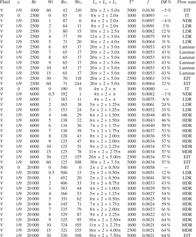
 $Wi = 0$ denotes Newtonian fluid) which covers a series of flow regimes including EIT, IT and DRT from the onset of DR to MDR, as well as the relaminarized flow regime by polymers. The other details of numerical conditions including some important results such as friction coefficient
 $f$, drag reduction rate
 $DR\,\%$ and flow state can be found in table 1, where
 $Re_\tau =h u_\tau /\nu$ and
 $We_\tau =\lambda u_\tau /h$ are friction Reynolds number and Weissenberg number using the friction velocity
 $u_\tau =\sqrt {\tau _w/\rho }$;
 $\tau _w$ is the mean shear stress at the wall and
 $\rho$ is the fluid density;
 $L_x \times L_y \times L_z$ is the channel sizes;
 $T^*$ denotes the total integration time for the statistical average values. For the datasets, the channel size for viscoelastic fluid flow is gradually modified empirically to accommodate the flow structures enlarged with the increase of
 $Wi$, including velocity streaks and polymer extension structures as shown in table 1. The total integration time is also increased from 1000 to 5000 as the flow enters MDR and even the EIT state due to the increase of time scale.
Calculation conditions. Here  $N$ and
 $V$ denote Newtonian and viscoelastic fluids, respectively; no drag reduction (NDR); low drag reduction (LDR); high drag reduction (HDR); drag-reducing flows with no DR effect (i.e. MDR);
 $0\,\% < {\rm DR}\,\% < 40\,\%, 40\,\% \le {\rm DR}\,\% < {\rm MDR}$ and
 ${\rm DR}\,\%={\rm MDR}$.

2.2. Budget equations
To understand the SSP of DRT, necessary budget equations including decompositions of ESS and pressure fluctuations involved are given below. Note that  $\bar {g}$ denotes an average of quantity
 $g$ over the
 $x$,
 $z$ and
 $t$ directions.
The Reynolds stress budget equation can be obtained by rearranging equation (2.2), as follows:
 \begin{equation} \frac{{\rm d} \overline{u'^{{*}_i}u'^{{{*}}}_j} }{{{\rm d} {t^*}}} ={P_{ij}^{{R}}}{{ + }}{\varPhi _{ij} }+{\varepsilon _{ij}^{{R}}}-{G_{ij} }+{T_{ij}^{{R}}},\end{equation}
where  ${P_{ij}^{{R}}= {-({\overline {u'^{* }_i u'^{* }_k } ({{{\rm d} \bar u^{* }_j }}/{{x_k^{* } }}) + \overline {u'^{* }_j u'^{* }_k } ({{{\rm d} \bar u_i^{* } }}/{{x_k^{* } }})})}}$ is the production rate;
 $\varPhi _{ij} = \overline {{{p'}^{* } }({{{\partial u'^{* }_j }}/{{\partial x_i^{* } }} + {{\partial u'^{* }_i }}/{{\partial x_j^{* }}}})}$ is the pressure-strain term;
 $\varepsilon _{ij}^{R}= {-({4}/{{{{Re}}}}) \overline {({{\partial u'^{* }_i }}/{{\partial x_k^{* } }})({{\partial u'^{* }_j }}/{{\partial x_k^{*}}})}}$ is the dissipation rate;
 $G_{ij}={({\overline {\tau '^{{{*}}} _{jk} ({{\partial u'^{{{*}}}_i}}/{{\partial x_k^{{{*}}}}})} + \overline {\tau '^{{{*}}} _{ik}({{\partial u'^{{{*}}}_j}}/{{\partial x_k^{{{*}}}}})}})}$ is the elastic stress–strain term;
 ${T_{ij}^{{R}}}=({{\rm d}}/{{\rm d} y^{*}})( - \overline {{u'}^{*}_{i}{u'}^{*}_{j}{v'}^{*}}+ \overline {{\tau '}^{*}_{j2}{u'}^{*}_{i}}+ \overline {{\tau ' }^{*}_{i2}{u'}^{*}_{j}}+({2}/{Re})({{\rm d}}/{{\rm d} y^{*}})\overline {{u'}^{*}_{i}{u'}^{*}_{j}})-({{\rm d} \overline {{{{{p'}}}^{*}}{u'}^{*}_{j}}}/{{\rm d}\kern0.06em x_{i}^{*}}+{{\rm d} \overline {{{{{p'}}}^{*}}{u'}^{*}_{i}}}/{{\rm d}\kern0.06em x_{j}^{*}})$ is the transport rate.
The pressure redistribution effect is an important link in turbulent SSP, responsible for the generation of TKE in the wall-normal direction. Following Ptasinski et al. (Reference Ptasinski, Boersma, Nieuwstadt, Hulsen, Van Den Brule and Hunt2003) and Terrapon et al. (Reference Terrapon, Dubief and Soria2015), the fluctuating pressure  $p'^*$ can be decomposed into rapid, slow and polymer contributions to investigate the modulation effect of polymers, as
 ${{{p'}^{* } }( \boldsymbol {x} ) = {p'}_R^{* } ( \boldsymbol {x} ) +{p'}_S^{* } ( \boldsymbol {x} ) +{p'}_P^{* } ( \boldsymbol {x} )}$ with
 ${{\boldsymbol x}=(x^*,y^*,z^*)}$, where
 \begin{equation} \left.\begin{array}{c@{}}
\dfrac{{{\partial ^2}p'^{* }_{{R}}}}{{{\partial}x_i^{ *
2}}} ={-} 2\dfrac{{{\rm d}{{\bar u}^*}}}{{{\rm d} {y^
*}}}\dfrac{{\partial v'^*}}{{\partial {x^ * }}},\\
\dfrac{{{\partial ^2}p'^{* }_{{S}} }}{{{\partial}x_i^{ *
2}}} ={-} \dfrac{{\partial u'^{* }_i }}{{\partial x_j^
*}}\dfrac{{\partial u'^{* }_j }}{{\partial x_i^ * }} +
\dfrac{{{{\rm d}^2}\overline{{{v'}^{ * 2}}} }}{{{\rm d}
{y^{ * 2}}}},\\ \dfrac{{{\partial ^2}p'^{* }_{{P}}
}}{{{\partial}x_i^{* 2}}} = \dfrac{{{\partial ^2}\tau'^{* }
_{ij} }}{{\partial x_i^* \partial x_j^*}},
\end{array}\right\} \end{equation}
and the first two are identified as inertial contributions.
The integral of the budget of TKE can be obtained by condensing equation (2.4) and implementing the integral operation,
 \begin{equation} P_{{k}}+\varepsilon_{{k}}-G=0,\end{equation}
where  ${P_{{k}} = - \int _0^2 {\overline {{{u'}^{*}}{{v'}^{*}}} ({{\partial {{\bar u}^ * }}}/{{\partial {y^ * }}})\, \textrm {d} {y^ *}}}$ is the global TKE production rate;
 $\varepsilon _{{k}} = -\int _0^2 ({2}/ {{{{Re}}}}) \overline {({{\partial u'^{*}_i}}/{{\partial x_j^{* } }})({{\partial u'^{* }_i }}/{{\partial x_j^{* } }})}\, \textrm {d} {y^*}$ is the global TKE dissipation rate;
 $G = \int _0^2 \overline {\tau '^{*} _{ij}({{\partial u'^{*}_i}}/{{\partial x_j^*}})} \, \textrm {d} {y^*}$ is the global energy transformation rate from TKE to turbulent elastic energy (TEE).
The elastic stress budget equation can be obtained by arranging equation (2.3), as follows:
 \begin{equation} \frac{{{\rm d} \bar \tau _{ij}^{* } }}{{{\rm d} {t^{* } }}} = {P_{ij}^{{E}}} +{G_{ij} }+{T_{ij}^{{E}}}{{ + }} {V_{ij} }+{\varepsilon _{ij}^{{E}}}, \end{equation}
where  ${P_{ij}^{{E}}}={({\bar \tau _{ik}^{*} ({{\textrm {d} \bar u_j^{*}}}/{{x_k^{* } }}) + \bar \tau _{kj}^{*} ({{\textrm {d} \bar u_i^{*}}}/{{x_k^{*}}})})}$ is the production rate;
 ${G_{ij} }$ is the elastic stress–strain term as in (2.4);
 ${T_{ij}^{{E}}}={-{{\textrm {d} \overline { v'^{* } \tau '^{* } _{ij} }}/{{{\textrm {d} y}^{*}}}}}$ is the turbulent transport rate;
 ${V_{ij}^ * ={({{2\gamma }}/{{{{Re}}\,{Wi}}})({{{\textrm {d} \bar u_j^{* } }}/{{x_i^{* }}} + {{\textrm {d} \bar u_i^{* }}}/{{x_j^{* } }}})}}$ is the viscous effect term;
 $\varepsilon _{ij}^{{E}}= - ( 1/Wi ) \bar \tau _{ij}^{*}$ is the elastic dissipation (relaxation) rate.
As the excitation of EIT is independent of the viscous effect term  ${V_{ij}^ *}$ in (2.7) which is a linear term, the mean ESS can be decomposed into the linear part of ESS (LESS)
 $\bar \tau _{E1}^ *$ and the nonlinear part of ESS (NESS)
 $\bar \tau _{E2}^ *$ (see Zhang et al. (Reference Zhang, Shao, Li, Ma, Zhang and Li2021a,Reference Zhang, Zhang, Li, Yu and Lib) for more information),
 \begin{equation} \bar \tau _E^ * = {\bar \tau _{E1}^ * } + {\bar \tau _{E2}^ * }, \end{equation}
where  $\bar \tau _{E1}^* \!=\!({\gamma }/{{{{Re}}}}) ({{\textrm {d} \bar u^*}}/{{\textrm {d} y^*}})$ ;
 $\bar \tau _{E2}^* =\! Wi( \bar \tau _{yy}^* ({{\textrm {d} \bar u^ * }}/{{\textrm {d} y^ * }}) \!+\! ( \overline {\tau '^{{ * }}_{1k}({{\partial v'^{* } }}/{{\partial x_k^ * }})} +\! \overline {\tau '^{*}_{k2} ({{\partial u'^{* } }}/{{\partial x_k^*}})}) - {{\textrm {d} \overline { u'^{*}_k \tau '^{* } _E }}/{{x_k^*}}})$ is caused by the interaction between polymers and turbulence. The nonlinear part of ESS
 ${\bar \tau _{E2}^*}$ is actually the so-called ‘stress loss’. Thus, the production term of elastic normal stress in the streamwise direction
 $\bar \tau _{xx}^ *$ can be decomposed into two parts based on (2.8),
 \begin{equation} P_{{xx}}^E=2\bar \tau _{E}^{* } \frac{{{\rm d} \bar u^{* } }}{{{{\rm d} y}^{* } }} = P_{{xx}}^{E1}+P_{{xx}}^{E2}, \end{equation}
where  $P_{{xx}}^{E1}=2\bar \tau _{E1}^{* } ({{\textrm {d} \bar u^{* } }}/{{{\textrm {d} y}^{* } }})$ is the linear part and
 $P_{{xx}}^{E2}=2\bar \tau _{E2}^{* } ({{\textrm {d} \bar u^{* } }}/{{{\textrm {d} y}^{* } }})$ is the nonlinear part. The integral of the budget of TEE can be obtained by condensing equation (2.7), arranging by using (2.8) and then implementing the integral operation,
 \begin{equation} P_{{e}}+\varepsilon_{{e}}+G=0, \end{equation}
where  ${P_{{e}} = - \int _0^2 {\bar \tau _{E2}^{{ * }}({{\partial {{\bar u}^ * }}}/{{\partial {y^ * }}})\, \textrm {d} {y^ * }} }$ is the global TEE production rate;
 $\varepsilon _{{e}} = -\int _0^2 (({1}/{{2Wi}}) \bar \tau _{ii}^{*}-\bar \tau _{E1}^{{*}} ({{\partial {{\bar u}^ * }}}/{{\partial {y^ * }}}))\, \textrm {d} {y^ *}$ is the global TEE dissipation rate.
3. Results and analysis
3.1. Statistical properties
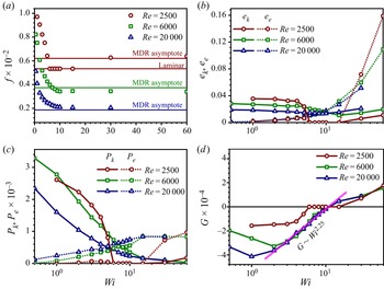
At first, we present some results for the flow statistics. Figure 1 illustrates friction coefficient  $f$, global TKE, global TEE, global TKE production rate
 $P_{k}=\int _0^2\bar \tau _{R}^* ({\textrm {d} \bar u^{*}}/{{{\textrm {d} y}^ * }})\, {\textrm {d} y}^*$ by Reynolds shear stress (RSS), global TEE production rate
 $P_{e}=\int _0^2\bar \tau _{E2}^* ({\textrm {d} \bar u^{*}}/{{{\textrm {d} y}^*}})\,{\textrm {d} y}^*$ by NESS as well as the global energy transfer rate
 $G=\int _0^2\overline {\tau '^*_{ij}({\partial {u'^*_i}}/{\partial {x^*_j}})}\,{\textrm {d} y}^*$ between TEE and TKE. The datasets qualitatively reproduce the interesting observations in Choueiri's experiments, which can be read from the evolutions of
 $f$ with
 $Wi$ in figure 1(a). The specific analysis is as follows.
Evolution of statistics with  $Wi$: (a) friction coefficient
 $f$; (b) global TKE
 $e_k$ and TEE
 $e_e$; (c) global TKE production
 ${P_{{k}} = - \int _0^2 {\overline {{{u'}^{* } }{{v'}^{* } }} ({{\partial {{\bar u}^ * }}}/{{\partial {y^ * }}})\, \textrm {d} {y^ * }} }$ and TEE production rate
 ${P_{{e}} = - \int _0^2 {\bar \tau _{E2}^{{ \ast }}({{\partial {{\bar u}^ * }}}/{{\partial {y^ * }}})\, \textrm {d} {y^ * }} }$; (d) global energy transformation rate
 ${G = \int _0^2 {\overline {\tau '^{*}_{ij} ({{\partial u'^{*}_i}}/{{\partial x_j^*}})} \, \textrm {d} {y^ * }} }$. The MDR asymptote of Virk (Reference Virk1975) in (a) is
 $f=0.58 {Re}^{-0.58}$. Here
 $G^* >0$ represents the energy that is globally transferred from polymers to the flow structures, otherwise from the flow structures to the polymers.

At moderate  $Re$ (e.g. 6000 or 20 000),
 $f$ continuously declines and finally converges to a certain value approaching the MDR asymptote of Virk (Reference Virk1975),
 $f=0.58{Re}^{-0.58}$. To be more specific, the viscoelastic turbulence experiences the onset of DR, LDR, HDR, MDR and EIT with the increase of
 $Wi$ according to the calculation results of
 $DR\,\%$ in table 1. In figure 1(b), global TKE gradually decreases before the flow enters the MDR stage, but begins to increase at a large
 $Wi$ (
 $Wi \approx 15$ for
 $Re=6000$ and
 $Wi \approx 10$ for
 $Re=20 000$); global TEE also turns to increase rapidly after the flow enters the MDR stage, compared with the slow increase before MDR. The above observations support the viewpoint that the underlying dynamics do not converge even after the flow enters the MDR stage reported by Zhu & Xi (Reference Zhu and Xi2021). We believe that the non-convergence results from the continuous evolution of EIT dynamics with
 $Wi$. Correspondingly, evolutions of
 ${P_{{k}}}$,
 ${P_{{e}} }$ and
 ${G }$ in figures 1(c) and 1(d) share similar trends for moderate
 $Re$. Since the onset of DR,
 ${P_{{k}}}$ starts to decrease, while
 ${P_{{e}}}$ starts to increase. When the flow enters the MDR and EIT regime,
 ${P_{{k}}}$ becomes negligible, whereas
 ${P_{{e}}}$ becomes dominant and saturated. During this process,
 $G$ first decreases to a valley and then starts to increase again with
 $Wi$. More strikingly, the value of
 $G$ is negative below the critical
 $Wi$ of MDR indicating the energy is globally transferred from TKE to TEE, but positive above the critical
 $Wi$ indicating the globally inverted energy transfer. Moreover, the evolution of
 $G$ after the valley point for the two
 $Re$ collapse to each other showing a power-law relationship with
 $Wi$ implying a scaling for
 $G$ independent of
 $Re$, which needs further investigations.
At a small  $Re$ (e.g. 2500), the flow experiences the regimes of the onset of DR, LDR, HDR, relaminarization and EIT (
 $Wi =30, 60$) regime as shown in figure 1(a). The existence of relaminarization for moderate
 $Wi$ (
 $\approx 6\text{--} 15$ in the current work) which distinguishes the dynamics of DRT in two different stages. Global TKE and TEE show similar evolution behaviours to those at moderate
 $Re$, except that they all disappear in the relaminarization window. Evolutions of
 ${P_{{k}} }$,
 ${P_{{e}}}$ and
 ${G}$ in figures 1(c) and 1(d) show different behaviours for low
 $Re$ compared with that for moderate
 $Re$. Before relaminarization,
 ${P_{{k}}}$ is dominant and the value of
 $G$ is always negative, indicating the turbulence is always IT-dominated which is inhibited by polymers; when the flow enters laminar regime for
 $Wi \approx 6\text{--} 15$,
 ${P_{{k}} }$,
 ${P_{{e}}}$ and
 ${G}$ become eliminated. In contrast, during the process of entering EIT,
 ${P_{{e}}}$ is dominant and the value of
 $G$ is positive for
 $Wi =30, 60$ indicating the turbulence is sustained by polymers.
The above results demonstrate a global picture for the elastic effect on the viscoelastic turbulence: (1) at small  $Wi$ (LDR for moderate
 $Re$ or before relaminarization for small
 $Re$), the flow is IT-dominated and in these cases the traditional TKE production by RSS is suppressed and thus IT-related SSP is modulated; (2) increasing
 $Wi$ above a critical value, a new TKE generation term induced by elastic effects appears, which grows with
 $Wi$ and changes the SSP in DRT; (3) further increasing
 $Wi$, the turbulence is changed from being sustained by
 $P_{k}$ to being sustained by
 $P_{e}$, and the nature of turbulence changes from polymer-modulated IT to EIT.
The characteristics of RSS attract the most attention in the comparison analysis between IT and DRT. What is unusual is that although there exist obvious velocity fluctuations (especially  $u'^*$) in EIT,
 $-\overline {{{u'}^{* }}{{v'}^{*}}}$ is extremely small, implying somehow the decoupling between
 $u'^*$ and
 $v'^*$. From our recent demonstrated SSP in EIT (Zhang et al. Reference Zhang, Zhang, Li, Yu and Li2021b), the energy picture including the TKE production in different directions and the embedded TKE transfer amongst them clearly differs from that of IT, which is possible to delay or decouple the generation of
 $u'^*$ from
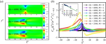
 $v'^*$. Figure 2 presents the negative cross-correlation between
 $u'^*$ and
 $v'^*$ over
 $x$,
 $z$ and
 $t$,
 $C_{uv}(y^*, \xi ^*)=-{\langle {u'^*( {x^*,y^*,z^*,t^*} )v'^*( {x^*+\xi ^*,y^*,z^*,t^*} )} \rangle }$. Strikingly, unlike that in IT, there exists an obvious phase shift between
 $u'^*$ and
 $v'^*$ in the HDR and EIT state: the maximum values of
 $C_{uv}(y^*, \xi ^*)$ all locate at
 $\xi ^*=0$ in IT but at some locations where
 $\xi ^*$ is less than zero, approximately
 $2h$ to
 $4h$ in figure 2(a). This means that the local cross-correlation between
 $u'^*$ and
 $v'^*$ is the strongest in IT, but
 $u'^*$ and upstream
 $v'^*$ is most relevant in EIT. Applying Taylor's frozen hypothesis, it further indicates
 $u'^*$ lags behind
 $v'^*$, somehow indicating that
 $v'^*$ induces the generation of
 $u'^*$. Moreover, in EIT, the lagging distance
 $\xi _{{max}}^*$ can reach several times the channel half-height
 $h$. For example, at
 $Re = 1000, Wi = 60, \xi _{{max}}^*$ can reach more than
 $5h$ in figure 2(b). In addition,
 $\xi _{{max}}^*$ gradually increases with an approximately linear relationship with
 $Wi$. The above results once again imply different pictures of the TKE transfer process between velocity components in IT and DRT.
Distributions of  $C_{uv}(y^*,\xi ^*)$: (a) in the
 $\xi$–
 $y$ plane; (b) at
 $y^* \approx 0.5$ and normalized by RSS here. Inset is
 $\xi _{{max}}^*$ versus
 $Wi$ at different
 $Re$. Here
 $\xi _{{max}}^*$ corresponds to the position where
 $C_{uv}(\xi ^*)$ reaches the maximum.

In the following, in-depth investigations on the link between EIT and DRT are carried out through analysis on structures, budgets and pressure fluctuations. Note that structures, budgets and pressure fluctuations are not shown at  $Re=20\,000$ for brevity because similar conclusions as those obtained at
 $Re = 6000$ can be drawn.
3.2. Structural analysis
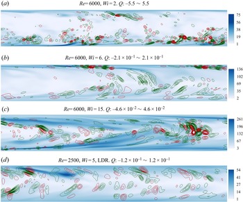
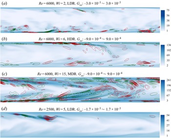
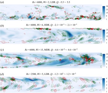
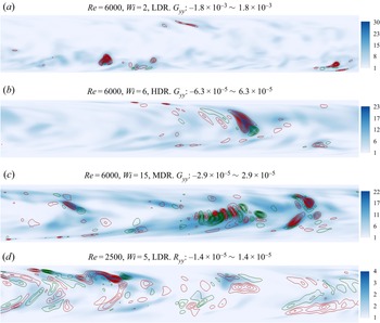
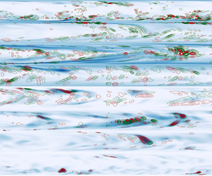
Figures 3–6 show the structure characteristics (sheet-like structures, spanwise vortexes and the interaction between polymers and turbulence) in the  $x$–
 $y$ plane of EIT and their performance in DRT, including instantaneous contours of streamwise and wall-normal polymer extension (
 $R_x=\sqrt {c_{xx}}$ and
 $R_y=\sqrt {c_{yy}}$, respectively), superimposed by the isolines of
 $G_{xx}$,
 $G_{yy}$ and
 $Q$, where
 $Q=(-1/2){\partial {_iu^*_j}}{\partial {_ju^*_i}}$ is the second invariant of the velocity gradient tensor. Note that these instantaneous results are extracted at high flow drag moment (namely, the active state in Xi & Graham (Reference Xi and Graham2010) and Dubief et al. (Reference Dubief, Terrapon and Soria2013)). The abscissa and ordinate of the subgraphs are
 $x^*$ and
 $y^*$, respectively, and the planes are properly compressed in the streamwise direction. Here
 $y^*$ uniformly ranges from 0 to 2, and
 $x^*$ ranges from 0 to
 $L_x$ (see table 1 for different channel lengths).
Instantaneous contours of streamwise polymer extension ( $R_x=\sqrt {c_{xx}}$) in the
 $x$–
 $y$ plane at active state. The superimposed isolines represent
 $Q$ in different subgraphs: green, negative; red, positive. The abscissa and ordinate of the subgraphs are
 $x^*$ and
 $y^*$ (from 0 to 2), respectively: (a)
 $x^*\in (0, 5{\rm \pi} )$; (b)
 $x^*\in (0, 7{\rm \pi} )$; (c)
 $x^*\in (0, 11{\rm \pi} )$; (d)
 $x^*\in (0, 16{\rm \pi} )$.

It can be observed from the instantaneous contours of  $R_x$ and
 $R_y$ at moderate
 $Re$ in these figures that (1) polymers are increasingly stretched with the increase of
 $Wi$ in both the streamwise and wall-normal directions; (2) sheet-like structures of streamwise polymer extension featured by EIT are activated at
 $Wi=6$, and further expanded to channel centre at
 $Wi=15$; (3) wall-normal polymer extension structures are also inclined from channel wall to channel centre along the streamwise direction but are not sheet-like, and these high extension structures shift from the channel wall at the LDR condition to the channel centre at the HDR and MDR conditions; (4) polymer extension structures between the streamwise and wall-normal directions are interrelated, and the relevance strengthens with the increase of
 $Wi$. At low
 $Re$, although streamwise polymer extension structures also incline from channel wall to channel centre at
 $Wi=5$ before laminarization, which are weakly correlated to wall-normal structures, they are less like thin sheets, which is more or less related to the plane compression in streamwise direction. It is notable that the sheet-like structures of polymer extension (especially in the streamwise direction) under the numerical conditions presented in this study (
 $Wi \le 15$) seem like they are originating from the near-wall region rather than the channel centre. This supports that the wall-mode instability (TS attractor) evolves to EIT, as reported by Shekar et al. (Reference Shekar, Mcmullen, Wang, Mckeon and Graham2019, Reference Shekar, Mcmullen, Mckeon and Graham2020, Reference Shekar, Mcmullen, Mckeon and Graham2021) in the present parameter space. Moreover, compared with that of streamwise polymer extension, the structures of wall-normal extension appear earlier near the channel centre (e.g. at
 $Wi = 15$), indicating the vortex structures are formed locally as shown in figure 5.
Two-dimensional projection of  $Q$ in the
 $x$–
 $y$ plane shows the spanwise vortex structures of DRT in figure 3 (or figure 5). At moderate
 $Re$, the LDR flow is filled with abundant small-scale spanwise vortex structures near the wall; these positive and negative vortexes are not related to polymer extension structures as in EIT; nearly circular and ellipse red isolines inclined from channel wall to channel centre are likely to be the two-dimensional projection of the three-dimensional hairpin vortex heads and legs in IT (see figure 3a). For low
 $Re$, these spanwise vortex structures are also weakly related to the polymer extension structures before laminarization at
 $Wi = 5$, but the scale of the vortex becomes larger (see figure 3d). After the flow enters the HDR state, the situation changes significantly (see figure 3b for the HDR state and figure 3c for the MDR state): it can be clearly found that the vortex structures are gradually lifted from the near wall to the centre region with the increase of
 $Wi$; at the near-wall region, small-scale spanwise vortex structures alternate sign around thin sheets of large polymer extension, indicating that the dynamics of EIT appear long before MDR; at the turbulent core region, large-scale spanwise vortex structures are found to be associated with the wall-normal extension structures, meaning that wall-normal polymer extension structures and the interaction with turbulent structures play important roles in EIT-related SSP.
Here,  $G_{xx}$ and
 $G_{yy}$ represent the energy conversion from TKE to TEE in the streamwise and wall-normal directions due to the interaction between polymer extension structures and turbulent structures, respectively. At
 $Re=6000$ and
 $Wi=2$, large energy conversion is mainly located at the near-wall region and plying-up with large polymer extension as shown in figures 4(a) and 6(a). Moreover, an obvious feature lies in the following: when large polymer extension structures begin to appear in the high shear region near the wall, related energy conversion is positive and polymers absorb energy from turbulent fluctuations leading to polymers’ coil-stretch transition; after extension structures are lifted to the turbulent core area,
 $G_{xx}$ turns to negative, that is, polymers relax and release energy to turbulence, which is consistent with the findings of Min, Choi & Yoo (Reference Min, Choi and Yoo2003). These phenomena can be also observed in figures 4(d) and 6(d), excepting that the structures of large
 $G_{yy}$ are lifted towards the channel centre likely due to broadened transition regions. After the flow enters the HDR state, the distribution pattern of
 $G_{xx}$ and
 $G_{yy}$ changes significantly in panels (b) and (c) of figures 4 and 6:
 $G_{xx}$ alternates its sign around sheet-like structures of high polymer extension, which is closely related to small-scale spanwise vortexes of
 $Q$ at the near-wall region; structures of large
 $G_{yy}$ gradually shift from the near-wall region to the turbulent core region and show strong correlation with large-scale spanwise vortexes of
 $Q$ there.
Instantaneous contours of streamwise polymer extension ( $R_x=\sqrt {c_{xx}}$) in the
 $x$–
 $y$ plane at active state. The superimposed isolines represent
 $G_{xx}$ in different subgraphs: green, negative; red, positive. The abscissa and ordinate of the subgraphs are
 $x^*$ and
 $y^*$ (from 0 to 2), respectively: (a)
 $x^*\in (0, 5{\rm \pi} )$; (b)
 $x^*\in (0, 7{\rm \pi} )$; (c)
 $x^*\in (0, 11{\rm \pi} )$; (d)
 $x^*\in (0, 16{\rm \pi} )$.

Instantaneous contours of wall-normal polymer extension in the  $x$–
 $y$ plane at active state. The superimposed isolines represent
 $Q$ in different subgraphs: green, negative; red, positive. The abscissa and ordinate of the subgraphs are
 $x^*$ and
 $y^*$ (from 0 to 2), respectively: (a)
 $x^*\in (0, 5{\rm \pi} )$; (b)
 $x^*\in (0, 7{\rm \pi} )$; (c)
 $x^*\in (0, 11{\rm \pi} )$; (d)
 $x^*\in (0, 16{\rm \pi} )$.

Instantaneous contours of wall-normal polymer extension in the  $x$–
 $y$ plane at active state. The superimposed isolines represent
 $G_{yy}$ in different subgraphs: green, negative; red, positive. The abscissa and ordinate of the subgraphs are
 $x^*$ and
 $y^*$ (from 0 to 2), respectively: (a)
 $x^*\in (0, 5{\rm \pi} )$; (b)
 $x^*\in (0, 7{\rm \pi} )$; (c)
 $x^*\in (0, 11{\rm \pi} )$; (d)
 $x^*\in (0, 16{\rm \pi} )$.

The above observations indicate that characteristic structures of EIT appear long before MDR, and that wall-normal polymer behaviours are also important in EIT dynamics. In order to further quantitatively reveal the correlation of the above important turbulent and polymer structures in DRT-related SSP, budget analysis is carried out in the next section.
3.3. Budget analysis
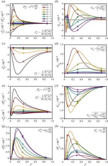
This section re-evaluates the energy transfer process in DRT by budget analysis of TKE, TEE and shear stresses between different components at moderate  $Re$ (
 $Re = 6000$) and low
 $Re$ (
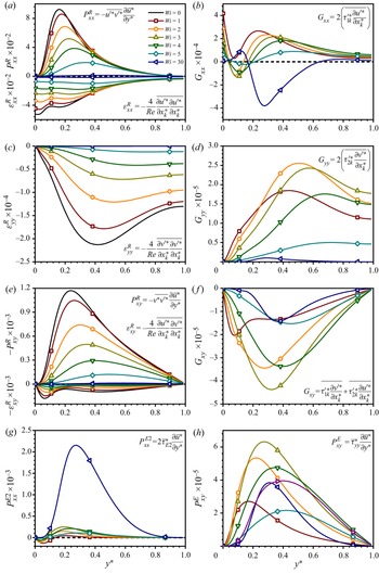
 $Re = 2500$), as illustrated in figures 7 and 8 considering whether the EIT-related SSP is formed. As is well known, in IT, RSS absorbs energy from the mean motion and produces streamwise TKE, which is transformed into wall-normal TKE through fast and slow pressure redistribution, and then regenerates RSS. The above process forms a cycle to maintain the turbulence against dissipative effects. As demonstrated in Zhang et al. (Reference Zhang, Zhang, Li, Yu and Li2021b), when the flow enters EIT, it follows a very different SSP. The most striking differences lie in: (1) rather than by RSS, NESS absorbs energy from the mean motion to sustain the turbulence; (2) the conversion of wall-normal TKE into TEE and streamwise TEE into TKE are added; (3) the interaction between polymers and turbulence suppresses both RSS and NESS. In addition, polymers also contribute to the energy redistribution in EIT which generates wall-normal TKE in the SSP cycle of EIT (Terrapon et al. Reference Terrapon, Dubief and Soria2015). Moreover, EIT-related SSP is possibly formed and survives from being dissipated once the above features appear. In the following, special attention is paid to the performance of terms related with these features.
Budgets analysis for  $\overline {{{u'}^{* }}{{u'}^{*}}}$,
 $\overline {{{v'}^{* }}{{v'}^{*}}}$,
 $\overline {{{u'}^{* }}{{v'}^{*}}}$,
 $\overline {\tau _{xx}^*}$,
 $\overline {\tau _{yy}^*}$ and
 $\overline {\tau _{xy}^*}$ at
 $Re=6000$, where
 ${P_{ij}^{{R}}}$ is Reynolds production rate;
 ${P_{ij}^{{E}}}$ is elastic production rate;
 ${\varepsilon _{ij}}$ is dissipation rate;
 ${G_{ij}}$ is elastic stress–strain term. Especially,
 ${P_{xx}^{{E2}}}=2\tau _{E2}\partial \bar u^*/\partial y^*$ is the elastic production by NESS.

Common with earlier studies (Xi Reference Xi2019), production and dissipation terms of Reynolds stresses such as  $P_{xx}^{{R}}$,
 $P_{xy}^{{R}}$ and
 $\epsilon _{xx}^{{R}}$,
 $\epsilon _{yy}^{{R}}$,
 $\epsilon _{xy}^{{R}}$ in panels (a), (c) and (e) of figures 7 and 8 gradually decrease with the increase of
 $Wi$, indicating the suppression of elasticity on the IT-related SSP in DRT. Moreover, it is observed from figures 7 and 8 that (1) at the moderate
 $Re$,
 $P_{xx}^{{E2}}$ continuously grows with
 $Wi$ and exceeds
 $P_{xx}^{{R}}$ almost everywhere at
 $Wi \approx 9$ if compared together, indicating that for cases at
 $Wi > 9$, more energy is transferred from the mean motion to polymers by NESS than that to turbulent structures and the turbulence is dominated by NESS; (2) at the small
 $Re$, the flow is dominated by
 $P_{xx}^{{R}}$ before the relaminarization while by
 $P_{xx}^{{E2}}$ when EIT is excited.
Budgets analysis for  $\overline {{{u'}^{* }}{{u'}^{*}}}$,
 $\overline {{{v'}^{* }}{{v'}^{*}}}$,
 $\overline {{{u'}^{* }}{{v'}^{*}}}$,
 $\overline {\tau _{xx}^*}$,
 $\overline {\tau _{yy}^*}$ and
 $\overline {\tau _{xy}^*}$ at
 $Re=2500$, where
 ${P_{ij}^{{R}}}$ is Reynolds production rate;
 ${P_{ij}^{{E}}}$ is elastic production rate;
 ${\varepsilon _{ij}}$ is dissipation rate;
 ${G_{ij}}$ is elastic stress–strain term. Especially,
 ${P_{xx}^{{E2}}}=2\tau _{E2}\partial \bar u^*/\partial y^*$ is the elastic production by NESS.

Interesting to notice from profiles of  $G_{xx}$ in figures 7(b) and 8(b) is that it experiences a morphological change with the increase of
 $Wi$. For a small
 $Wi$ (e.g. at
 $Re=6000, Wi = 2$ and
 $Re=2500, Wi = 5$), energy is transferred from streamwise TKE to TEE in the bulk region, which increases with
 $Wi$ and introduces additional energy loss. This effect modulates the IT-related SSP. For moderate and large
 $Wi$ (e.g. at
 $Re=6000, Wi > 4$ and
 $Re=2500, Wi =30, 60$ after the emergence of the EIT regime), the energy transfer direction turns over with the increase of
 $Wi$. The negative energy transfer region (from TEE to TKE) shifts from the near-wall region to the bulk region, and enlarges with
 $Wi$. Meanwhile, the positive energy transfer region (from TKE to TEE) shifts from the bulk region to the near-wall region, and shrinks with
 $Wi$. Notable is that the region where polymers absorb energy shifts upward with
 $Wi$, which probably originates from turbulent streaks lifting, as reported in Zhang et al. (Reference Zhang, Zhang, Li, Yu and Li2021b). The core area is mainly characterized by the energy transfer of TEE to TKE, which indicates that EIT dynamics can be self-sustained, i.e. EIT-related SSP involved. With the increase of
 $Wi$, more TEE is transferred from polymers to TKE until the flow completely develops into EIT. Compared with
 $G_{xx}$, the energy transfer rate
 $G_{yy}$ between
 $\overline {{{v'}^{* }}{{v'}^{*}}}$ and
 $\bar \tau _{yy}^*$ is negative for all the covered viscoelastic flow regimes (see figures 7d and 8d), indicating that polymers always suppress the wall-normal turbulence. With the increase of
 $Wi$, as
 $\overline {{{v'}^{* }}{{v'}^{*}}}$ is suppressed by polymers, less energy is transferred from TKE to TEE.
The evolutions of  $P^{R}_{xy}$ are illustrated in figures 7(e) and 8(e). Originating from the production of wall-normal TKE and the mean shear, this term dominates the gain effect of RSS. Similarly, it decreases with
 $Wi$ due to suppression of wall-normal TKE in DRT. Interestingly, the term
 $G_{xy}$ is always negative throughout all DR stages as shown in figures 7( f) and 8( f), implying that the interaction between polymers and turbulence shows a dual suppressing effect on the RSS and also NESS. At last, the budget of NESS is analysed by focusing on the term of
 $P^{E}_{xy}$ as shown in figures 7(h) and 8(h), induced by the production of wall-normal extension and the mean shear similar to the RSS production term
 $P^{R}_{xy}$. Unlike
 $P^{R}_{xy}$,
 $P^{E}_{xy}$ first increases with
 $Wi$ and then dampens in DRT. This can be attributed to the behaviour of
 $\tau _{yy}$, induced by the interaction between polymers and turbulence, which on the one hand is enlarged by the increase of elasticity, and on the other is reduced due to the suppression of the turbulence.
3.4. Pressure and its redistribution effect
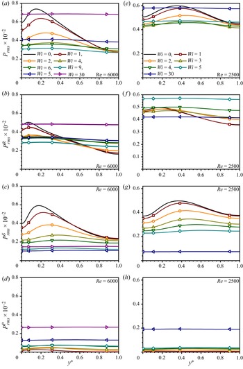
Pressure fluctuations in wall turbulence play an important role in the redistribution of TKE in different directions. As is shown in equation (2.5), the rapid and slow pressure fluctuations are induced by the deformation of the mean flow field and turbulent interaction, respectively. As Terrapon et al. (Reference Terrapon, Dubief and Soria2015) reported, the rapid contribution represents the immediate response to a change imposed on the mean flow field, while the slow part feels this change through nonlinear interactions. In addition, the polymeric pressure fluctuations are due to the polymeric stress fluctuations. Therefore, in Ptasinski et al. (2003) and Terrapon et al. (Reference Terrapon, Dubief and Soria2015), the first two parts (rapid and slow contributions) and the third part are intuitively identified to be inertial and elastic, respectively. This is necessary to be reconfirmed here since it is related to determining which dynamics dominates the pressure redistribution effect, IT or EIT. To this end, the root mean square (r.m.s.) values of total, fast, slow and polymeric pressure at the same moderate  $Re (= 6000)$ with Terrapon et al. (Reference Terrapon, Dubief and Soria2015) as well as low
 $Re (= 2500)$ across the bottom channel height are shown in figure 9.
Pressure r.m.s. as a function of  $y^*$: (a–d) total, rapid, slow and polymeric contribution (see panel (a) for legend) at
 $Re=6000$; (e–h) total, rapid, slow and polymeric contribution (see panel (e) for legend) at
 $Re=2500$.

For moderate  $Re$, compared with Newtonian IT, when
 $Wi$ increases to a certain value (e.g.
 $Wi = 9$),
 $p_{rms}$ of DRT turns into quasi-flat distribution (see figure 9a), which well reproduces the observation in the simulation by Terrapon et al. (Reference Terrapon, Dubief and Soria2015). It can be also found that
 $p_{rms}$ generally shows a downward trend with the increase of
 $Wi$ at first, and then begins to rise when the flow enters the MDR state (e.g.
 $Wi = 9$), which greatly implies the transformation of dominant dynamics in DRT. Comparing the distribution patterns of fast, slow and polymeric contributions, it can be seen that the fast contribution shows a similar development law with the total contribution, indicating that the pattern change of
 $p_{rms}$ is mainly affected by the fast contribution. In Newtonian IT abundant turbulent fluctuations and coherent structures locate in the near-wall region (especially in the buffer layer), which can well explain the single hump distribution pattern of
 $p_{rms}$ with the near-wall peak. In contrast, EIT is excited from the centre-mode instability and is affected by both the wall-mode and the centre mode at moderate and high
 $Re$ (see Choueiri et al. Reference Choueiri, Lopez, Varshney, Sankar and Hof2021), which can qualitatively explain the reason for the quasi-flat distribution pattern of
 $p_{rms}$. The fast contribution represents the interaction between turbulent fluctuations and mean motion, while the slow contribution reflects the turbulence–turbulence interaction. From figures 9(b) and 9(c), it appears that (1) both distributions of fast contribution and slow contribution become more and more flat with the enhancement of the DR effect; (2) they all completely become the quasi-flat distribution featured by EIT after the flow enters the MDR state. The above phenomena show that the inertial nature of fast and slow pressure fluctuations are likely to be gradually replaced by an elastic nature with the increase of
 $Wi$, because elastic nonlinearity gradually replaces inertial nonlinearity to generate turbulent fluctuations during this process. For
 $p_{rms}^{P}$ in figure 9(d), the distribution also shows a quasi-flat pattern after the flow enters MDR state (e.g.
 $Wi = 9$). Interestingly, at the LDR state (e.g.
 $Wi = 1$, 2), it shows a single hump distribution with near-wall peak similar to fast and slow contributions. The evolution behaviour shows that with the increase of
 $Wi$, polymeric pressure fluctuations also experience the transformation from inertial nature to elastic nature, considering that polymers can be significantly stretched by interacting with coherent structures in IT near the wall.
For low  $Re$, compared with the cases at moderate
 $Re$, the peak positions of
 $p_{rms}$,
 $p_{rms}^R$ and
 $p_{rms}^S$ of IT move away from the wall; the r.m.s. value decreases at the channel wall and rises at the channel centre. With the increase of
 $Wi$, the total pressure fluctuations also gradually decrease and become flatter and flatter, and finally show a quasi-flat distribution at
 $Wi = 5$ before laminarization, similar to that in EIT. We speculate that the elasto-inertial instability may be triggered intermittently at
 $Wi = 5$, but cannot sustain itself. Similar to the cases at moderate
 $Re$, slow pressure fluctuations are gradually suppressed. When
 $Wi \ge 4$, the r.m.s. value of rapid pressure fluctuations begins to increase abnormally, which may be a unique phenomenon of slugs in the flows, because they are higher than the r.m.s. value in EIT at
 $Wi = 30$; moreover, the r.m.s. value of fast pressure fluctuations is even higher than that of total pressure fluctuations, indicating that part of the fast pressure fluctuations offsets part of the slow ones. Before entering the laminar state, polymeric pressure fluctuations are very weak and r.m.s. values are almost zero. For EIT at
 $Wi = 30$, the r.m.s. values of total, fast, slow and polymeric pressure fluctuations all show a quasi-flat pattern and lower than those at moderate
 $Re$. Prominently,
 $p_{rms}^R$ at
 $Wi=30$ is much higher than that in the flow before the window of relaminarization.
In short, through the above analysis of the distribution pattern of the r.m.s. value of pressure, we speculate that the fast, slow and polymeric pressure fluctuations can behave with both inertial and elastic nature, which depends on the dominating nonlinear dynamics in DRT. In the following, we focus on the pressure redistribution term related with fast, slow and polymeric effects in the budgets to understand the role of pressure redistribution in the link between DRT and EIT.
Different from  $\overline {{{u'}^{* }}{{u'}^{*}}}$, the generation of
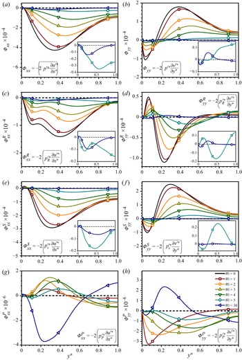
 $\overline {{{v'}^{* }}{{v'}^{*}}}$ is from pressure redistribution. Figures 10 and 11 show the evolutions of total, rapid, slow and polymeric pressure redistribution terms under different flow conditions. In IT both
 $\varPhi _{xx}^{{R}}$ and
 $\varPhi _{xx}^{{S}}$ behave as negative in the turbulent core area, i.e. TKE is redistributed to other directions from streamwise direction through slow and fast pressure fluctuations; the behaviour of
 $\varPhi _{yy}^{{S}}$ is opposite to that of
 $\varPhi _{xx}^{{S}}$ but this is not the case for
 $\varPhi _{yy}^{{R}}$: near the wall (at approximately
 $y^* < 0.1$),
 $\varPhi _{yy}$ is negative, indicating the energy is redistributed to the streamwise direction forming turbulent streaks and in turbulent core region (at approximately
 $y^* > 0.1$),
 $\varPhi _{yy}$ is positive, indicating the energy is redistributed to the wall-normal direction and forms
 $\overline {{{v'}^{* }}{{v'}^{*}}}$.
Profiles of total pressure distribution at  $Re=6000$ on
 $\overline {{{u'}^{* }}{{u'}^{*}}}$,
 $\overline {{{v'}^{* }}{{v'}^{*}}}$ and the divided rapid, slow and elastic contributions (see panel (h) for legend), where
 ${\varPhi _{xx} =2{\overline {{{p'}^{* } }({{{\partial u'^{* } }}/{{\partial x^{* } }}} )} }}$;
 ${\varPhi _{yy} =2{\overline {{{p'}^{* } }( {{{\partial v'^{* } }}/{{\partial y^{* } }}} )} }}$;
 ${{{p'}^{* } }( \boldsymbol {x} ) = {p'}_R^{* } ( \boldsymbol {x} ) +{p'}_S^{* } ( \boldsymbol {x} ) +{p'}_P^{* } ( \boldsymbol {x} )}$.

In DRT at moderate  $Re$ in figure 10, for small
 $Wi$ when the turbulence is IT-dominated, both
 $\varPhi ^{{R}}$ and
 $\varPhi ^{{S}}$ are far larger than
 $\varPhi ^{{P}}$ in both the streamwise and wall-normal directions, and
 $\varPhi ^{{P}}_{yy}$ does not generate but consumes
 $\overline {{{v'}^{* }}{{v'}^{*}}}$. With the increase of
 $Wi$,
 $\varPhi ^{{P}}$ of an active elastic nature is gradually excited and generates
 $\overline {{{v'}^{* }}{{v'}^{*}}}$ on one hand, and
 $\varPhi ^{{R}}$ and
 $\varPhi ^{{S}}$ are dampened on the other hand. When
 $Wi$ is large enough,
 $\varPhi ^{{P}}$ catches up with those two terms, and can affect the total pressure redistribution. Strikingly, the evolutions of
 $\varPhi ^{{P}}$ demonstrate a similar trend with that of
 $G_{xx}$ and
 $P^{E2}_{xx}$ with the increase of
 $Wi$. For cases of small
 $Wi$, e.g.
 $Wi = 2$ at
 $Re = 6000$,
 $\varPhi _{yy}^{{P}}$ is small and negative, i.e.
 $\overline {{{v'}^{* }}{{v'}^{*}}}$ is transferred to other directions through
 $\varPhi _{yy}^{{P}}$. However, for large
 $Wi$, e.g.
 $Wi \ge 4$ at
 $Re = 6000$, there is an obvious positive polymer effect near the wall, i.e. TKE in other directions is transferred to the wall-normal direction through
 $\varPhi _{yy}^{{P}}$. Polymers play a gain effect on the normal-wise TKE generation which sustains
 $\overline {{{v'}^{* }}{{v'}^{*}}}$ and turbulent SSP. Therefore, polymers introduce a new pressure redistribution mechanism in DRT. It plays a modulation effect on pressure redistribution when
 $Wi$ is small, but can reshape the pressure redistribution effect when
 $Wi$ is large enough, making the correlation between
 ${u'}^{*}$ and
 ${v'}^{*}$ in DRT more complex. When entering EIT, the characteristics of the pressure redistribution effect are obviously different from that in IT, and the polymeric contribution plays an indispensable role in generating
 ${v'}^{*}$. Although it is speculated in the previous section that the slow and fast contributions are likely to be driven by elastic nonlinearity rather than inertial nonlinearity at high
 $Wi$, in any case, the morphological transformation of pressure redistribution by polymers is the most notable feature for EIT-related SSP.
In DRT at low  $Re$ in figure 11, there exist some distinctions from the cases at moderate
 $Re$. Before the relaminarization phenomenon occurs (e.g.
 $Wi \leq 5$), both
 $\varPhi ^{{R}}$ and
 $\varPhi ^{{S}}$ in the
 $x$ and
 $y$ directions are also far larger than
 $\varPhi ^{{P}}$, and polymeric pressure fluctuations redistribute wall-normal TKE to other directions. But the morphological transformation of
 $\varPhi ^{{P}}$ does not occur until
 $Wi=5$. With the increase of
 $Wi$,
 $\varPhi ^{{R}}$ and
 $\varPhi ^{{S}}$ are dampened, but always much higher than
 $\varPhi ^{{P}}$, which is also broadly suppressed with the decline of IT in the wall-normal direction. At
 $Wi = 5$, the polymeric pressure redistribution effect still does not catch up with slow and rapid ones, and consequently does not show morphological change. In other words, the pressure redistribution effect featured by EIT is not excited before relaminarization, and polymeric pressure fluctuations at this stage are a passive response to IT dynamics, similar to these under LDR conditions at moderate
 $Re$ (e.g.
 $Wi=1,2$ for
 $Re=6000$). When an instability appears and the flow enters EIT from the laminar regime, pressure fluctuations induced by polymers begin to generate wall-normal velocity fluctuations and play an indispensable role in energy SSP (see figures 11g and 11h). Moreover,
 $\varPhi ^{{R}}_{yy}$ in figure 11(d) extraordinarily shows morphological inversion: it is positive at near-wall region (at approximately
 $y^*<0.12$) and negative at part of turbulent core region (at approximately
 $0.12< y^*<0.55$) in Newtonian IT, but show the opposite effects in roughly the same regions in EIT. Again, this transformation from consumption to generation of
 $\overline {{{v'}^{* }}{{v'}^{*}}}$ implies rapid pressure fluctuations experience the change from inertial nature to elastic nature.
Profiles of total pressure distribution at  $Re=2500$ on
 $\overline {{{u'}^{* }}{{u'}^{*}}}$,
 $\overline {{{v'}^{* }}{{v'}^{*}}}$ and the divided rapid, slow and elastic contributions (see panel (h) for legend), where
 ${\varPhi _{xx} =2{\overline {{{p'}^{* } }( {{{\partial u'^{* } }}/{{\partial x^{* } }}} )} }}$;
 ${\varPhi _{yy} =2{\overline {{{p'}^{* } }( {{{\partial v'^{* } }}/{{\partial y^{* } }}} )} }}$;
 ${{{p'}^{* } }( \boldsymbol {x} ) = {p'}_R^{* } ( \boldsymbol {x} ) +{p'}_S^{* } ( \boldsymbol {x} ) +{p'}_P^{* } ( \boldsymbol {x} )}$.

From the above budget analysis, there exists a distinct SSP from IT in viscoelastic DRT. On the one hand, the existence of elastic effect suppresses the self-sustaining mechanism related to IT. On the other hand, when  $Wi$ is large enough, a cycle of EIT-related SSP is introduced, which finally replaces that of IT.
3.5. Repicturing viscoelastic DRT
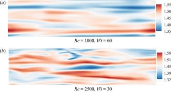
Based on the above analysis, we repicture the energy process for viscoelastic DRT from IT to EIT by combing energy and stress budgets as shown in Figure 12. First, the cycles of energy SSP for IT and EIT are illustrated by the cyan paths in figure 12(a) and the blue paths attached by cyan dashed paths in figure 12(d), respectively. Classical understanding about energy SSP of IT is that RSS absorbs energy from the mean motion and converts it into streamwise TKE, part of which is further redistributed to wall-normal TKE through pressure fluctuations, and then regenerates RSS. In this study, the energy SSP of EIT is further updated relative to our previous work (see Zhang et al. Reference Zhang, Shao, Li, Ma, Zhang and Li2021a). Specifically, a similar energy SSP of IT is added with cyan dashed paths, considering these paths still exist weakly in the so-called EIT regime. Here, we speculate these paths are a passive response to the SSP of EIT, similar to the passive response of polymers to the energy SSP of IT at the LDR state (see discussion about the energy process at the LDR state in figure 12b, below). These paths may be responsible for the three-dimensional structures in EIT, such as the velocity streaks (see figure 13) distributed in the  $x$–
 $z$ plane similar to streaks in ET (see Jha & Steinberg Reference Jha and Steinberg2021). The difference lies in that these paths do not seem to inhibit EIT, but are likely to boost EIT. For example, fast and slow pressure fluctuations can help to regenerate wall-normal velocity fluctuations, although it is uncertain whether these velocity fluctuations will participate in the EIT-related SSP. In this case, the converged friction coefficient independent of the increase of
 $Wi$ in EIT needs to find other reasons, such as the negative feedback regulation of suppression effect on NESS due to the interaction between polymers and turbulence,
 $G_{xy}$. The energy SSP in two-dimensional EIT will provide an important reference to solve these problems, which is a research work we are carrying out.
Energy picture of viscoelastic DRT: —— (cyan) and —— (blue), SSP cycles in IT and EIT, respectively; —— (orange), the bypass of energy process caused by the passive response of polymers on IT; —— (red), energy source and dissipation.

Instantaneous contours of streamwise velocity in the  $x$–
 $z$ plane close to the channel centre. The abscissa and ordinate of the subgraphs are
 $x^*$ (from 0 to 20
 ${\rm \pi}$) and
 $z^*$ (from 0 to 5
 ${\rm \pi}$), respectively.

The energy process in DRT from onset of DR to MDR, is illustrated in figure 12(b) for early LDR conditions and in figure 12(c) for later LDR, HDR and early MDR conditions. Under early LDR conditions (e.g.  $Wi = 1, 2$ for
 $Re=6000$), polymers passively respond to the SSP of IT with orange paths. The TKE is partially transformed into TEE through the interaction between polymers and turbulence in both the streamwise and wall-normal directions. In addition, partial streamwise TEE in a very small region near the channel walls is transformed into TKE. The NESS is formed due to a wall-normal polymer extension. The NESS absorbs energy from mean motion and turns into streamwise TEE. The above process is a passive response to the SSP of IT, which cannot support but significantly interferes its SSP. Pressure fluctuations induced by polymers distribute TKE from the wall-normal direction to other directions such as the streamwise, opposing that of fast and slow pressure distributions although with almost negligible magnitude. Moreover, there is an orange path showing the interaction between polymers and turbulence, which inhibits both RSS and NESS and is another important factor for polymers to interfere the SSP of IT. When
 $Wi$ is high enough (e.g.
 $Wi=4$ at
 $Re=6000$), the energy process of EIT begins to intervene and coexist with that of IT disturbed by polymers in figure 12(c). This coexistent phase sustains from later LDR conditions to early MDR conditions at least. With the increase of
 $Wi$, the energy process of DRT gradually transits to that of the EIT state. In this process, the IT-related SSP weakens and the EIT-related SSP gradually dominates the flow.
In Choueiri et al. (Reference Choueiri, Lopez and Hof2018), it was believed that elasto-inertial instability sets in before complete relaminarization at moderate  $Re$, resulting in a mixed state which then eventually approaches MDR. With the above energy picture in mind, the different DR phenomena at low
 $Re$ and moderate
 $Re$ can be well unified and the underlying mechanism can be further confirmed. As shown in figure 12, the two important links related with energy SSP cycle of EIT described by
 $G_{xx}$ (see figures 7b and 8b) and
 $\varPhi ^P_{yy}$ (see figures 10h and 11h) can be well hold at
 $Wi = 4$ for
 $Re = 6000$ but are not formed even at
 $Wi = 5$ for
 $Re = 2500$. That is to say, with the increase of
 $Re$, the triggering of EIT becomes easier since smaller fluid elasticity is required at higher
 $Re$. On the one hand, IT becomes more difficult to be suppressed as
 $Re$ increases since the streamwise vortices are stronger, so it takes larger fluid elasticity (or higher
 $Wi$) to suppress them (see Li, Xi & Graham Reference Li, Xi and Graham2006; Li & Graham Reference Li and Graham2007). In short, whether laminarization will occur or not needs to comprehensive consideration of the above two effects. That is, with the increase of
 $Re$, EIT becomes easier to trigger but IT becomes more difficult to suppress. Thus, consistent with Choueiri et al. (Reference Choueiri, Lopez and Hof2018), when
 $Wi$ is further increased, the flow is laminarized at
 $Re = 2500$ since the weaker IT disappears before EIT (the so-called ‘barrier to laminarization’ in Zhu & Xi (Reference Zhu and Xi2021) is excited, whereas, the flow directly enters EIT regime at
 $Re = 6000$ without a window of relaminarization as EIT-related SSP can be well sustained before IT-related SSP completely disappears).
Looking back at figure 1(c), the following explanation about the valley of  $G$ distribution at low
 $Wi$ (
 $Wi \approx 2$ for
 $Re=6000$ and
 $Wi \approx 1$ for
 $Re=20\,000$) can be given based on the proposed energy process in figure 12. For the cases before the valley, the EIT-related SSP has not been formed because the two necessary links of
 $G_{xx}$ (see figure 7b for
 $Re=6000$) and
 $\varPhi ^P_{yy}$ (see figure 10h for
 $Re=6000$) are not yet formed, and polymers passively participate in the IT-related SSP, absorbing energy from turbulence and converting it into TEE. Here
 $G$ denotes the energy conversion between TKE and TEE through the interaction between polymers and turbulence, that is, work done by fluctuating polymer stress depending on both the strength of fluid elasticity and turbulence intensity. On the one hand, the enhancement of fluid elasticity (the increase of
 $Wi$) is conducive to enhanced interaction, which increases the magnitude of
 $G$. On the other hand, with the enhancement of the DR effect due to the increase of fluid elasticity, IT is significantly inhibited, which suppresses the interaction before EIT is formed. In addition, EIT begins to intervene in DRT almost at the end of the valley, which introduces reverse energy transfer from TEE to TKE. As a result, the valley is formed under the confrontation of the above three effects.
We can also further understand the reason why  $u'^*$ lags behind
 $v'^*$ in DRT observed in figure 2. In IT, DRT and EIT, the formation of
 $u'^*$ are all inseparable with
 $v'^*$ but with a different routine. In IT, the energy absorbed by RSS sustains the formation of
 $u'^*$. The formed TKE in the streamwise direction is then redistributed to
 $v'^*$ directly through the pressure redistribution effect. The formation of
 $u'^*$ and the energy redistribution to
 $v'$ are direct processes and rapid terms. However, in the DRT and EIT regime, polymers even change the formation mechanism of
 $u'^*$, as illustrated by the orange path and blue path in figure 8. Different from that in IT,
 $u'^*$ is mainly derived from the conversion of streamwise TEE in the EIT regime, and the generation of streamwise TEE is from the wall-normal TEE caused by
 $v'^*$. Due to the polymer-memory effect, the formation and development of this process are indirect and takes a certain time, related to the fluid relaxation time, which results in the phenomenon
 $u'^*$ lags behind
 $v'^*$. For DRT, with the increase of
 $Wi$, the IT-related SSP gradually weakens, while the EIT-related SSP enhances and the time memory effect increases, resulting in the phenomenon that the lag distance increases.
4. Conclusions and future works
In summary, we have repictured viscoelastic DRT in channels, especially its energy transfer process, based on statistical and budget analysis throughout a wide range of flow states covering IT, LDR, HDR, MDR to EIT and the relaminarized flow regime. The evolutionary comparison of  $e_{k}, e_{e}, P_{k}, P_{e}$ and
 $G$ with
 $Wi$ provide quantitative evidence that the nature of DRT gradually changes from IT to EIT. The statistical results of
 $C_{uv}$ between IT, DRT and EIT are in sharp contrast, which further implies that there exists an SSP different from IT in DRT. Fast, slow and polymeric pressure fluctuations are likely to have dual natures. Specifically, with the enhancement of fluid elasticity, they gradually change from an inertial nature to an elastic nature. For energy and stress budget, polymers do have the passive feedback effect of modulating and interfering with the IT-related SSP, but more importantly, when
 $Wi$ exceeds a certain critical value long before the flow enters the MDR state, polymers can actively excite EIT-related SSP. The two obvious characteristics of this active behaviour are that polymers pump energy from mean motion to induce streamwise turbulent fluctuations, and that polymers can induce the pressure distribution to provide energy for the formation of wall-normal turbulent fluctuations. These evidences fully suggest that the nature of DRT experienced the transition from pure IT, IT modulated by polymers, participation of EIT and finally maybe pure EIT. The different DR phenomena at low
 $Re$ (e.g.
 $Re=2500$) and moderate
 $Re$ (e.g.
 $Re=6000, 20\,000$) are unified through the proposed energy picture. The reason why the relaminarized phenomenon does not occur at moderate
 $Re$ is further confirmed by the fact that inertial nonlinearity is stronger than that at low
 $Re$, and EIT dynamics gets involved in the flow earlier before IT dynamics completely disappear through stronger polymeric suppression, so that the turbulence can be maintained and fed by elasticity instability. In other words, the flow is relaminarized at low
 $Re$ with the coherent structures of IT are completely destroyed by polymers when the barrier of EIT dynamics against laminarization is not yet established.
The proposed energy picture provides a theoretical foundation for DRT modelling in the future, and also illustrates why the existing DRT models cannot well predict HDR and MDR flows since EIT dynamics are not involved. In addition, the connection is important to the further understanding of viscoelastic DRT and EIT. To this end, special attention in this study is paid to the possible relation of structures of polymer extension and vortex structures to the energy transfer term. They do show underlying links between them. However, we have to admit that it is not easy to build a direct and impressive connection between the budgets and structures in the current flow conditions as too many processes are cross-linked together. A systematic investigation focusing on this topic needs to be conducted from various aspects to simultaneously capture the evolution of the structures and the detailed energy transfer process for cases from its origin of EIT to the fully developed case. However, as the target of this paper is to repicture the drag-reducing turbulence, we would like to put this into our future work.
Acknowledgements
The authors are grateful to the reviewers for the constructive suggestions on this paper.
Funding
This research was funded by the National Natural Science Foundation of China (NSFC 51976238, 51776057, 52006249).
Declaration of interests
The authors report no conflict of interest.