



1. Introduction
Pulsatile turbulent pipe flows are widely encountered in engineering applications and biological systems, such as the turbomachinery and blood flow in aortic arteries. The oscillating nature of the pulsatile flow leads to a high-level fluctuation of the wall friction. Understanding the variation of the wall shear stress is of great practical significance to, e.g. pipeline leak detections (Colombo, Lee & Karney Reference Colombo, Lee and Karney2009) and blood-vessel problems (Cunningham & Gotlieb Reference Cunningham and Gotlieb2005), which require precise knowledge of flow dynamic behaviours. This paper is concerned with the wall shear stresses in pulsatile turbulent pipe flows and the corresponding fluid dynamics.
The pulsation process consists of continuous accelerating and decelerating phases. In the past decades, several researchers have focused on the flow responses in the accelerating turbulent pipe or channel flow, in which the flow rate varies in a step- or ramp-changing manner (Maruyama, Kuribayashi & Mizushina Reference Maruyama, Kuribayashi and Mizushina1976; Greenblatt & Moss Reference Greenblatt and Moss1999; He & Jackson Reference He and Jackson2000; Greenblatt & Moss Reference Greenblatt and Moss2004). It is well established, in both scenarios, that the flow initially evolves in a laminar-like way, accompanied by the streamwise stretching of the near-wall streaks (stage 1). Then, the elongated streaks break up, leading to the formation and subsequent merging of turbulent spots (stage 2). Finally, the turbulence reaches its new fully developed state (stage 3) (He, Ariyaratne & Vardy Reference He, Ariyaratne and Vardy2011; Jung & Chung Reference Jung and Chung2012; Seddighi et al. Reference Seddighi, He, Vardy and Orlandi2014; He & Seddighi Reference He and Seddighi2015; He, Seddighi & He Reference He, Seddighi and He2016). Specifically, this three-stage flow evolution resembles closely the bypass transition in the boundary layer induced by the free stream turbulence (He & Seddighi Reference He and Seddighi2013). Mathur et al. (Reference Mathur, Gorji, He, Seddighi, Vardy, O'Donoghue and Pokrajac2018) interpreted this process in a different way by regarding the preexisting turbulence as a perturbation that leads to the instability of the temporally developing laminar boundary layer from the wall. In any case, the laminar-like flow behaviours at the early stage allow an unsteady friction model to be established to predict the wall shear stress. Based on the assumption that the turbulence in stage 1 is nearly ‘frozen’, He & Ariyaratne (Reference He and Ariyaratne2011) derived a laminar-flow formulation to describe the wall shear stress at that stage. The acquired results are in good agreement with experimental or computational outcomes as further consolidated by He et al. (Reference He, Ariyaratne and Vardy2011). He & Seddighi (Reference He and Seddighi2015) and Jung & Kim (Reference Jung and Kim2017) discussed the effects of the ratio of the final to initial Reynolds number and the effects of the acceleration rate on the transition, respectively. They both showed that the turbulence evolves progressively for a low ratio and low acceleration rate, which is in contrast to the aforementioned bypass transition. Guerrero, Lambert & Chin (Reference Guerrero, Lambert and Chin2021) investigated the transient dynamics of the accelerating turbulent pipe flow in detail. By using the FIK identity, which is an exact expression developed by Fukagata, Iwamoto & Kasagi (Reference Fukagata, Iwamoto and Kasagi2002) to quantify the friction coefficient for wall-bounded flows, they were able to quantify the different contributions to the wall friction during the transient. Moreover, Sundstrom & Cervantes (Reference Sundstrom and Cervantes2018a) showed that the flow responses during the accelerating phase of the pulsatile flow are similar to those in the first two stages of the uniformly accelerating flow. As for the decelerating flow which is characterized by a decay of the preexisting turbulence (Mathur Reference Mathur2016), Sundstrom & Cervantes (Reference Sundstrom and Cervantes2018c) also demonstrated its laminar similarity to the accelerating flow at the initial stage.
Different from the one-way flow excursion reviewed above, the pulsatile turbulent flow exhibits strong wave–turbulence interactions due to the shear wave generated near the wall. The laminar Stokes thickness  $l_{s}^{+}=l_{s}\bar {u}_{\tau }/\nu, l_{s} =\sqrt {2\nu /\omega }$, where
 $\nu$ and
 $\omega$ are the kinematic viscosity and the angular pulsatile frequency, respectively, is generally used to characterize the wall-normal length scale of such a near-wall shear wave. In the present paper, the superscript
 $+$ denotes normalization using the mean friction velocity
 $\bar {u}_\tau$ and the kinematic viscosity
 $\nu$. To take into account the diffusion effect of turbulence, Scotti & Piomelli (Reference Scotti and Piomelli2001) proposed a turbulent Stokes thickness
 $l_{t}$, based on the eddy-viscosity theory, as the scaling parameter. There have been several experimental studies that focused on the pulsatile flows (Gerrard Reference Gerrard1971; Ronneberger & Ahrens Reference Ronneberger and Ahrens1977; Ramaprian & Tu Reference Ramaprian and Tu1980, Reference Ramaprian and Tu1983; Tu & Ramaprian Reference Tu and Ramaprian1983; Shemer & Kit Reference Shemer and Kit1984; Shemer, Wygnanski & Kit Reference Shemer, Wygnanski and Kit1985; Mao & Hanratty Reference Mao and Hanratty1986; Tardu & Binder Reference Tardu and Binder1993; Tardu, Binder & Blackwelder Reference Tardu, Binder and Blackwelder1994; Lodahl, Sumer & Fredsøe Reference Lodahl, Sumer and Fredsøe1998; He & Jackson Reference He and Jackson2009), covering a wide range of pulsation parameters. The wave–turbulence interactions exhibit a strong frequency dependence. When the pulsation frequency is high (
 $0.02\lesssim \omega ^+ \lesssim 0.04$), the Stokes thickness is small such that the shear wave is only confined to the very narrow near-wall region. In this case, the inner shear wave and outer turbulence are weakly coupled (quasi-laminar state). There is a
 $45^\circ$ phase lag between the centreline velocity and the wall shear stress, which coincides with the laminar Stokes solution. When the frequency falls in a low-frequency range (
 $\omega ^+\lesssim 0.005$), the flow variation is slow enough to allow the turbulence to react and settle down. Hence, the instantaneous flow field resembles that of the steady flow at the corresponding Reynolds number (quasi-steady state). Generally speaking, if the pulsation amplitude is not large enough to induce a reversal flow, the time-averaged flow quantities remain nearly unchanged from their values in the steady flow (Brereton, Reynolds & Jayaraman Reference Brereton, Reynolds and Jayaraman1990). However, Tu & Ramaprian (Reference Tu and Ramaprian1983) showed a deviation of the mean velocity profile from the steady one when the frequency is close to or larger than the turbulent bursting frequency in the turbulent pipe flow, i.e. a very-high frequency range (
 $\omega ^+\gtrsim 0.04$). This can be possibly attributed to a resonance effect with the closeness between the pulsation frequency and the characteristic frequency of the near-wall coherent structure. In contrast, Tardu et al. (Reference Tardu, Binder and Blackwelder1994) and Scotti & Piomelli (Reference Scotti and Piomelli2001) did not report such a deviation in turbulent channel flows with different pulsation parameters. This might be due to the dependency of the bursting frequency on the Reynolds number and geometry such that a resonance condition is not easily satisfied. Sundstrom, Mulu & Cervantes (Reference Sundstrom, Mulu and Cervantes2016) performed experimental research on a double-frequency pulsatile turbulent pipe flow and showed that the time-averaged flow quantities are also unaffected by the double-frequency pulsation. For a large-amplitude oscillation (usually refers to a situation when the oscillatory to mean velocity ratio
 $A$ is larger than one), Manna, Vacca & Verzicco (Reference Manna, Vacca and Verzicco2012) reported a drag-reducing effect which manifests as an upward shift of the mean velocity profile in the logarithmic region. This is consistent with Mao & Hanratty (Reference Mao and Hanratty1994) and Manna & Vacca (Reference Manna and Vacca2005) in which a reduction of wall shear stresses was both reported.
The laminar–turbulent transition is also an important phenomenon that occurs in pulsatile flows. Turbulence can be completely relaminarized in the pulsatile pipe flow with a non-zero mean flow under certain parameters (Lodahl et al. Reference Lodahl, Sumer and Fredsøe1998), and can also appear intermittently in a purely oscillatory flow (Feldmann & Wagner Reference Feldmann and Wagner2012), which belongs to a subcritical transition scenario (Feldmann & Wagner Reference Feldmann and Wagner2016b). Xu et al. (Reference Xu, Warnecke, Song, Ma and Hof2017) conducted an experimental study on the transition in a pulsatile pipe at amplitudes  $A\le 0.7$. Based on the transition theory in the steady pipe flow (Hof et al. Reference Hof, Westerweel, Schneider and Eckhardt2006; Avila, Willis & Hof Reference Avila, Willis and Hof2010; Avila et al. Reference Avila, Moxey, De Lozar, Avila, Barkley and Hof2011), they summarized the effects of pulsation frequency and this was further elaborated by Xu & Avila (Reference Xu and Avila2018) with the aid of the direct numerical simulation (DNS). For a large-amplitude pulsation with
 $A> 0.7$, Xu, Song & Avila (Reference Xu, Song and Avila2021); Xu et al. (Reference Xu, Varshney, Ma, Song, Riedl, Avila and Hof2020) reported a helical instability mechanism that induces the burst of turbulence in a pulsatile pipe flow. In particular, this helical disturbance is triggered during the decelerating phase and disappears in the accelerating phase, indicating a strong phase asymmetry in the pulsatile pipe flow (Feldmann & Wagner Reference Feldmann and Wagner2016a). Further, Morón, Feldmann & Avila (Reference Morón, Feldmann and Avila2022) linked this helical instability to the linear stability of the corresponding laminar flow and discussed the effect of the pulsation wave form on the turbulence transition. Similarly, Feldmann, Morón & Avila (Reference Feldmann, Morón and Avila2020) investigated the spatio-temporal intermittency associated with a competition between the helical structures and puffs. This intermittency in the pulsatile pipe flow is qualitatively similar to the gas-liquid slug pipe flow reported by Padrino et al. (Reference Padrino, Srinil, Kurushina and Swailes2023).
A paradoxical phenomenon occurs in the intermediate frequency range ( $0.005\lesssim \omega ^+\lesssim 0.02$). In this frequency range, the amplitude of the oscillating wall shear stress in a turbulent flow (
 $A_{\widetilde {\tau _{w}},t}$) is smaller than that in a laminar flow with the same pulsation conditions (
 $A_{\widetilde {\tau _{w}},s}$). This suggests a turbulence-induced drag reduction that is opposite to that in the steady flow where turbulence generally produces a larger drag than a laminar flow (Mao & Hanratty Reference Mao and Hanratty1986; Tardu et al. Reference Tardu, Binder and Blackwelder1994; Sundstrom & Cervantes Reference Sundstrom and Cervantes2018a). To deal with a non-closure problem in the governing equation, several researchers have established theoretical models for the Reynolds shear stress based on the concept of eddy viscosity. Most of these models in general fail to describe accurately the paradoxical phenomenon due to the inherent assumption that the Reynolds shear stress is in phase with the imposed oscillation (Weng, Boij & Hanifi Reference Weng, Boij and Hanifi2016; Weng, Boij & Hanifi Reference Weng, Boij and Hanifi2013). Weng et al. (Reference Weng, Boij and Hanifi2016) introduced the time dependency of the Reynolds shear stress into the standard eddy-viscosity model, which brings a phase lag between the Reynolds shear stress and the oscillating shear strain rate. This improved model is shown to be able to predict correctly the paradoxical phenomenon. However, a detailed explanation on why and how the turbulence reduces the wall shear stress is still lacking. Sundstrom & Cervantes (Reference Sundstrom and Cervantes2018b) provided a new interpretation of this paradoxical phenomenon by decomposing the total wall shear stress into the contributions from the oscillating pressure gradient (
 $\tau _p$) and the Reynolds shear stress (
 $\tau _s$). It is shown that a phase shift between
 $\tau _p$ and
 $\tau _s$ results in a mutual cancellation that leads to the reduction of the total wall shear stress. Nevertheless, in their experimental study,
 $\tau _s$ is calculated by subtracting
 $\tau _p$ from the measured total wall shear stress while
 $\tau _p$ is calculated by the laminar Stokes solution. Hence, this interpretation still cannot explain the underlying mechanisms; for instance, it does not explain what causes the phase shift. Based on these, we choose to perform direct numerical simulations in turbulent pulsatile pipe flows, in the hope of extending the numerical database of pulsatile flows, elucidating the physical mechanisms that cause the paradoxical phenomenon and revealing the corresponding turbulence dynamics in detail.
This paper is organized as follows. A computational set-up is introduced in § 2. Some basic statistics and the properties of the varying wall shear stress are given in § 3. Section 4 explores the causes of the paradoxical phenomenon and § 5 discusses the hysteresis phenomenon of the wall shear stress. The effects of the pulsation amplitude are examined in § 6. Section 7 further examines the phase-wise variation of spectra and § 8 summarizes the main findings of this paper.
2. Computational set-up
For pulsatile flows, it is common to introduce a triple decomposition of the flow quantity  $f(\boldsymbol {x},t)$ (Hussain & Reynolds Reference Hussain and Reynolds1970; Weng et al. Reference Weng, Boij and Hanifi2016; Sundstrom & Cervantes Reference Sundstrom and Cervantes2018b):
 \begin{equation} f(\boldsymbol{x},t)=\left \langle\, f \right \rangle (\boldsymbol{x},\varphi) + f'(\boldsymbol{x},t)=\bar{f} (\boldsymbol{x})+\tilde{f}(\boldsymbol{x},\varphi)+f'(\boldsymbol{x},t), \end{equation}
where  $\bar {f}$ and
 $\langle\, f \rangle$ are the time-averaged and phase-averaged values,
 $\tilde {f}$ is the oscillating component,
 $f'$ is the turbulent fluctuation and
 $\varphi$ is the phase. By further including the spatial average in statistically homogeneous directions, the time and phase averages can be defined as
 \begin{gather} \left\langle\, {f} \right\rangle(y,\varphi) = \lim_{M \to \infty } \frac{1}{{2{\rm \pi} ML}}\sum_{n = 1}^M {\int_0^L {\int_0^{2{\rm \pi} } {f\left(\boldsymbol{x},t + \frac{2{\rm \pi} n}{\omega}\right)} } } \,{\rm d}\kern 0.06em x\,{\rm d}\theta, \end{gather}
 \begin{gather} \bar{f} (y) = \int_0^{2{\rm \pi}} {\left\langle\, f \right\rangle } (y,\varphi )\,{\rm d}\varphi, \end{gather}
where  $x$,
 $y=R-r$ and
 $\theta$ denote the streamwise, wall-normal and azimuthal directions, respectively, with the corresponding velocity components being
 $u$,
 $-v$ and
 $w$. The pipe radius is
 $R$,
 $L$ is the pipe length and
 $M$ is the total number of periods.
In the present study, the pulsation is achieved by imposing a sinusoidally varying component to the constant streamwise pressure gradient that drives the steady turbulent pipe flow:
 \begin{equation} \frac{\partial p}{\partial x}(t)=\frac{\partial \bar{p}}{\partial x}(1+\beta \sin(\omega t)). \end{equation}
The constant mean pressure gradient  $\partial \bar {p}/{\partial x}$ is set to aim for a steady turbulent flow of
 $Re_\tau =\bar {u}_\tau R/\nu =180$. Throughout the paper, the quantity
 $\varphi$ refers to a phase of the streamwise pressure gradient
 $\partial p/\partial x$. We use the ratio of the amplitude of the oscillating velocity to the mean velocity at the pipe centreline, i.e.
 $A=A_{\tilde {u}_{cl}}/\bar {u}_{cl}$, to characterize the pulsation amplitude. Using (2.1), the governing equation for the oscillating component of the streamwise velocity reads:
 \begin{equation} \frac{\partial \tilde{u}}{\partial t}={-}\frac{\partial \tilde{p}}{\partial x}+ \nu \frac{1}{r} \frac{\partial \tilde{u}}{\partial r} +\nu \frac{\partial ^2 \tilde{u} }{\partial r^2} \underbrace{-\frac{\partial r\widetilde{u'v'} }{r\partial r}}_{\wp}. \end{equation}
By evaluating (2.4) at the pipe centreline, we have
 \begin{equation} A={-}\frac{\partial \bar{p}}{\partial x}\frac{\beta }{\omega }. \end{equation}
Hence,  $\beta$ can be predetermined based on the desired pulsation amplitude
 $A$.
To enable a direct comparison, the pulsation parameters selected in this paper, which are given in table 1, are similar to those of Weng et al. (Reference Weng, Boij and Hanifi2016) and Sundstrom & Cervantes (Reference Sundstrom and Cervantes2018b) (figure 1a). Five frequencies are chosen for  $A=0.1$ (Cases 1–5), and the resulting Womersley numbers
 $W=R\sqrt {\omega /\nu }$ ranges from 12.7 to 63.6. In addition, simulations of Cases 6 and 7 are performed at a higher amplitude of
 $A=0.4$ to evaluate the effect of pulsation amplitude. To provide a more comprehensive comparison with previous studies, each case is plotted in the
 $Re_b\unicode{x2013}Re_w$ plane (Lodahl et al. Reference Lodahl, Sumer and Fredsøe1998) together with available literature data (figure 1b). Here,
 $Re_b=U_bD/\nu$ is the bulk Reynolds number based on the bulk velocity
 $U_b$ and the pipe diameter
 $D$, and
 $Re_w={A_{\tilde {u}_{cl}}}^2/\omega \nu$ is the oscillatory Reynolds number. It is clear that all cases fall in the turbulent regime, as demonstrated in figure 3 where the instantaneous streamwise velocity at the meridional plane for Case 7 is shown. Although there is a large coincidence in the parameter space between the current study and Cheng et al. (Reference Cheng, Jelly, Illingworth, Marusic and Ooi2020), we note that our goal is not to carry out an investigation in the unexplored parameter space but to further elucidate the mechanisms responsible for the aforementioned paradoxical phenomenon based on existing parameters in the literature. Further, all the simulation cases of Cheng et al. (Reference Cheng, Jelly, Illingworth, Marusic and Ooi2020) are conducted at the fixed
 $\beta$ while the pulsation amplitude
 $A$ is fixed in the present study. Therefore, our cases are in fact different from those of Cheng et al. (Reference Cheng, Jelly, Illingworth, Marusic and Ooi2020) according to (2.5). For each case, the pulsation is imposed at a single flow field of the steady turbulent pipe flow. After discarding the transient effect, the phase-averaged data are collected over more than 23 periods to obtain the final statistics.
Cases with different pulsation parameters, namely the pulsation amplitude  $A$, the frequency
 $\omega ^+$. Here,
 $l_s^{+}$ is the laminar Stokes thickness;
 $W$ is the Womersley number;
 $A_{\widetilde {\tau _{w}},t}/A_{\widetilde {\tau _{w}},s}$ is the amplitude of the wall shear stress normalized by its laminar Stokes value; and
 $Re_b=U_bD/\nu$ and
 $Re_w={A_{\tilde {u}_{cl}}}^2/\omega \nu$ are the bulk and oscillatory Reynolds numbers, respectively.

(a) Variation of the amplitude of the wall shear stress  $A_{\widetilde {\tau _{w}},t}$ normalized by the laminar Stokes amplitude
 $A_{\widetilde {\tau _{w}},s}$ with respect to the laminar Stokes thickness
 $l_s^+$. (b) Laminar–turbulent transition boundary (dash-dotted line, Lodahl et al. Reference Lodahl, Sumer and Fredsøe1998) and parameter combinations considered by previous studies. The critical Reynolds numbers
 $Re_{b,tr}$ and
 $Re_{w,tr}$ are denoted by the dashed lines.

A cylindrical-coordinate spectral element–Fourier DNS solver Semtex is employed to conduct the simulations (Blackburn & Sherwin Reference Blackburn and Sherwin2004; Blackburn et al. Reference Blackburn, Lee, Albrecht and Singh2019). The computational mesh is the same as that of Liu et al. (Reference Liu, Zhu, Bao, Zhou and Han2022), where a  $50\times 10$ two-dimensional spectral element mesh is deployed to discretize the meridional semi-plane. To represent the three-dimensional computational domain, 192 Fourier expansion planes are used in the azimuthal direction. The pipe length is set to be
 $L=6{\rm \pi} R$. To ensure that this mesh configuration is appropriate to resolve the precise turbulence dynamics, we choose Cases 3 and 7 to conduct the mesh independence test. The choice of these two cases is based on the fact that the former is the case for which the ratio
 $A_{\widetilde {\tau _{w}},t}/A_{\widetilde {\tau _{w}},s}$ reaches its minimum and the latter is a high-amplitude case in which the variation of turbulence dynamics is more intense. Details of the spatial grid resolution are given in table 2. The
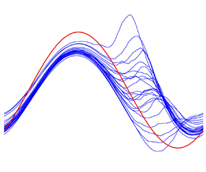
 $hp$-refinement strategy for the spectral element method is employed. Our baseline grid resolutions are comparable with the regular and high resolutions reported by Zahtila et al. (Reference Zahtila, Lu, Chan and Ooi2023). Figure 2 shows the phase-averaged wall shear stress obtained from various grids. It can be found that all the curves for Case 3 overlap well and the kink variation trend in Case 7 can be observed for all test cases, indicating that our phase-averaged statistics are grid independent. Figure 1(a) compares the present results of
 $A_{\widetilde {\tau _{w}},t}/A_{\widetilde {\tau _{w}},s}$ for
 $A=0.1$ with previous studies. It is shown that the paradoxical phenomenon can be clearly reproduced and that the variation trend of
 $A_{\widetilde {\tau _{w}},t}/A_{\widetilde {\tau _{w}},s}$ with respect to
 $l_s^+$ is also consistent with that in the literature. Note that the temporal variation of the wall shear stress is not necessarily a pure sine function; thus, here the amplitude corresponds to the amplitude of the fundamental mode calculated from the Fourier analysis. Quantitatively, a reasonable agreement can also be found except that the minimum of
 $A_{\widetilde {\tau _{w}},t}/A_{\widetilde {\tau _{w}},s}$ is 0.65 at
 $l_s^+=14$, which is smaller compared with that of Weng et al. (Reference Weng, Boij and Hanifi2016) and Sundstrom & Cervantes (Reference Sundstrom and Cervantes2018b) but in agreement with Tardu et al. (Reference Tardu, Binder and Blackwelder1994). This can probably be attributed to the different Reynolds numbers used in these studies. Moreover, the instantaneous fields in figure 3 exhibit visual smoothness, and no mesh imprints can be found. Hence, these results give us confidence in the accuracy of the DNS data used in this paper.
Summary of the grid information. Here,  $\Delta x^+$,
 $\Delta y^+$ are the normalized streamwise, wall-normal grid resolutions;
 $\Delta (r\theta )_{wall}^+$ is the normalized circumferential grid resolution at the wall;
 $P$ is the number of Lagrange knot points along the side of each element, corresponding to a polynomial order of
 $P-1$;
 $N$ represents the number of Fourier expansion planes in the circumferential direction;
 $H$ denotes the number of elements in the streamwise direction, which is associated with the streamwise
 $h$-refinement strategy in the spectral element method.

Comparisons of the phase-averaged wall shear stress  $\langle \tau _w\rangle$ between different mesh-independence validation cases: (a) Case 3 (
 $A=0.1$,
 $l_s^+=14$); (b) Case 7 (
 $A=0.4$,
 $l_s^+=17$).

Contours of the instantaneous inner-scaled streamwise velocity  $u^{+}$ in the meridional plane for Case 7 (
 $A=0.4$,
 $l_s^+=17$) at (a)
 $\varphi \approx 0$, (b)
 $\varphi \approx {\rm \pi}/4$, (c)
 $\varphi \approx {\rm \pi}/2$, (d)
 $\varphi \approx 3{\rm \pi} /4$.

3. Fundamental characteristics of pulsatile flow
First, we present some basic properties of the pulsatile pipe flow. Figure 4(a) shows the oscillating component of the streamwise velocity at the pipe centreline  $\tilde {u}_{cl}$. As expected, the oscillating amplitudes for high-frequency cases (Cases 2 and 3) are exactly
 $A=0.1$, while they are slightly larger than 0.1 for low-frequency cases (Cases 4 and 5). This is due to the strong coupling of the near-wall shear layer and the central region for low-frequency cases (Weng et al. Reference Weng, Boij and Hanifi2016). A similar phenomenon can also be found for higher amplitude cases where the centreline velocity oscillates at an amplitude larger than 0.4 for Case 7. Figure 4(b,c) shows the wall-normal profiles of the normalized mean velocity
 $\bar {u}$ and the components of the Reynolds stress tensor. The mean velocity is insensitive to the frequency at a low amplitude of
 $A=0.1$, but an increase in amplitude leads to the elevation of
 $\bar {u}$ in the log region. This is consistent with previous studies (Scotti & Piomelli Reference Scotti and Piomelli2001; Manna et al. Reference Manna, Vacca and Verzicco2012). In addition, the mean velocity seems to be more sensitive to the frequency for high-amplitude cases. For the presented Reynolds stresses, all the curves collapse well except for that of
 $\overline {u'u'}$. The increase of amplitude produces a larger magnitude of
 $\overline {u'u'}$ beyond
 $y^+\approx 10$, and
 $\overline {u'u'}$ is insensitive to the frequency for low-amplitude cases. Furthermore, the increase of
 $\overline {u'u'}$ is accompanied by the wall-normal location of the maximum
 $\overline {u'u'}$ moving away from the wall, which is similar to the situation where a transverse Stokes layer is generated by the wall oscillation (Quadrio & Sibilla Reference Quadrio and Sibilla2000; Liu et al. Reference Liu, Zhu, Bao, Zhou and Han2022).
(a) Time evolution of the oscillating component of the streamwise velocity  $\tilde {u}_{cl}$ at the pipe centreline. (b) Wall-normal profiles of the mean streamwise velocity
 $\bar {u}^{+}$. (c) Wall-normal profiles of the components of the Reynolds stress tensor. Note that the curves for the steady pipe (no pulsation) overlap completely with those for Case 2 in panel (b,c).

The near-wall flow dynamics is directly reflected by the wall shear stress. Figure 5 compares the phase-wise variation of the wall shear stress  $\widetilde {\tau _w}$ (black solid lines) with their corresponding laminar Stokes values (dashed blue lines) for cases with
 $A=0.1$, with the latter calculated by evaluating the radial derivative of the laminar Stokes solution at the wall (see Manna et al. Reference Manna, Vacca and Verzicco2012):
 \begin{equation} \tilde{u}(r,t) = A\,{\cdot}\, {\rm Re} \left[{\rm i}\left(\frac{{{{\rm J}_0}({{\rm i}^{3/2}}\sqrt 2 r/{l_s})}}{{{{\rm J}_0}({{\rm i}^{3/2}}\sqrt 2 R/{l_s})}} - 1\right){{\rm e}^{{\rm i}\omega (t - T/4)}}\right], \end{equation}
where  ${\rm J}_{0}$ is the Bessel function of the first kind of order zero, Re[
 $\,{\cdot}\,$] represents the real part of the argument,
 ${\rm i}$ is the imaginary unit and
 $T$ is the pulsation period. Also included is the corresponding fundamental mode obtained from the Fourier analysis (red solid lines), which allows us to evaluate qualitatively the extent of the nonlinear effect due to the turbulence. For a better presentation of the variation tendency, the data are duplicated and then spliced such that two periods are shown.
Phase-wise variations of the oscillating component of the wall shear stress  $\widetilde {\tau _w}$ for
 $A=0.1$ (the black lines), with the corresponding fundamental Fourier mode represented by the red solid lines. The blue dashed lines correspond to the laminar Stokes solution. The vertical arrows denote the phases where the phase-averaged wall shear stress
 $\langle \tau _w \rangle$ reaches its maximum or minimum. (a) Case 1; (b) Case 2; (c) Case 3; (d) Case 4; (e) Case 5.

For Case 1, the three curves overlap completely, indicating a quasi-laminar flow state. The phase-wise variation of the wall shear stress follows a purely sinusoidal pattern (figure 5a). A mild increase in frequency leads to the subtle departure from the laminar Stokes value and the decrease of  $A_{\widetilde {\tau _{w}},t}/A_{\widetilde {\tau _{w}},s}$ from unity for Case 2 (figure 5b). For Case 3, it is clear that the amplitude of the wall shear stress is significantly smaller than its laminar value but they still synchronize in phase. The differences between the wall shear stress and its fundamental mode are subtle, suggesting that the phase symmetry still holds. Considerable changes occur for Case 4. As seen, the wall shear stress deviates significantly from its fundamental mode. The drag-increasing phase occupies for a longer portion of the cycle than the drag-decreasing phase. That is, a hysteresis occurs during the oscillation cycle, indicating the destruction of the phase symmetry. Interestingly, when approaching the maxima, the increasing rate decreases, leading to a stage of the high-level wall shear stress with a slow growth. Similar phenomena have also been reported experimentally by Sundstrom & Cervantes (Reference Sundstrom and Cervantes2018b), where up to 500 cycles of measurements have been performed to obtain the phase-averaged wall shear stress at a higher amplitude and Reynolds number. Nevertheless, their data still suffer from fluctuations due to measurement uncertainties. Chen et al. (Reference Chen, Chan, Hutchins, Poon and Ooi2014) also reported the same tendency for similar pulsation parameters, but their data were obtained only from the final period. In the present study, the sufficient number of averaging periods and the spatial average in homogeneous directions ensure the smoothness of the phase-averaged statistics. In addition, the wall shear stress lags behind the laminar value, which does not occur in the former cases. This discrepancy and the physical meaning of this phase lag will be discussed in § 5. For the smallest frequency considered (Case 5), the deviations from the fundamental mode are still observable and the hysteresis is less evident but discernable. A phase lag with respect to the laminar value can also be observed. Theoretically, if the frequency is small enough to reach the quasi-steady state, all three curves should be in phase with the sinusoidally varying pressure gradient, and no hysteresis occurs. Hence, it can be inferred that as the frequency increases from zero, the aforementioned phase lag and hysteresis emerge initially and then disappear gradually.
Figure 6 shows the phase-wise variation of the wall shear stress for cases with  $A=0.4$. A reduction of the amplitudes compared with the corresponding laminar value is still observable. Specifically,
 $A_{\widetilde {\tau _{w}},t}/A_{\widetilde {\tau _{w}},s}$ increases from 0.65 to 0.8 as the amplitude increases from 0.1 to 0.4 for
 $l_s^+=14$, while it decreases from 0.86 to 0.59 for
 $l_s^+=17$. For Case 6, a distinct deviation from the fundamental mode occurs when the wall shear stress reaches its minimum (negative peak of
 $\widetilde {\tau _w}$), which implies a strong nonlinear effect of turbulence at that phase. Same as that for
 $A=0.1$, the wall shear stress is still in phase with the laminar value. For Case 7, a distinct kink can be clearly observed at around the phase of
 $t=3T/4$. We note that both Tu & Ramaprian (Reference Tu and Ramaprian1983) and Scotti & Piomelli (Reference Scotti and Piomelli2001) reported such a kink, but the causes are still unclear. Such a kink also implies special turbulence dynamics and will be discussed in detail in § 6. The fundamental mode lags behind the laminar value, consistent with that for
 $A=0.1$. It is worth noting that we only consider a higher amplitude at two intermediate frequencies. In fact, increasing the amplitude will not change the quasi-laminar state for high-frequency cases (e.g. Cases 1 and 2), hence their wall shear stresses are expected to still follow the laminar solution; while for a low-frequency case where the quasi-steady state is reached, a higher pulsation amplitude leads to a higher amplitude of the wall shear stress, but the variation trend would still follow a sinusoidal manner. Case 5 can be considered as a transition case for which the flow state is closer to the quasi-steady state. The hysteresis phenomenon at the frequency of Case 5 with a higher amplitude is probably not evident. Thus, behaviours of the wall shear stress for cases with high or low frequencies are somewhat predictable, which is the reason for considering only these two frequencies with a higher amplitude.
Phase-wise variations of the oscillating component of the wall shear stress  $\widetilde {\tau _w}$ for
 $A=0.4$ (the black lines), with the corresponding fundamental Fourier mode represented by the red solid lines. The blue dashed lines correspond to the laminar Stokes solution. The vertical arrows denote the phases where the phase-averaged wall shear stress
 $\langle \tau _w \rangle$ reaches its maximum or minimum. (a) Case 6; (b) Case 7.

In this section, we provide a general description of the pulsatile pipe flow, with a focus on the phase-wise variation of the wall shear stress. Different combinations of the pulsation parameters lead to significantly different behaviours of  $\widetilde {\tau _w}$. In the following sections, we aim to explore the causes of such differences and the corresponding flow dynamics based on (2.4) since
 $\widetilde {\tau _w}$ correlates closely to
 $\tilde {u}$ near the wall.
4. Damping mechanisms of the oscillating wall shear stress
We focus on Case 3, for which the ratio  $A_{\widetilde {\tau _{w}},t}/A_{\widetilde {\tau _{w}},s}$ reaches its minimum, to elucidate the mechanisms that lead to the amplitude reduction of the oscillating wall shear stress (
 $\widetilde {\tau _w}$) in the turbulent state compared with its corresponding laminar value.
The phase-wise variation of  $\tilde {u}$ for Case 3 is shown in figure 7(b), together with its laminar value calculated from (3.1) shown in figure 7(a). As seen, the most dramatic difference resides in the near-wall region; namely, below
 $y^+\approx 20$, the laminar contour appears to be more distorted than that in the turbulent case in that region. By examining the contour values, it can be observed that the amplitude of the oscillating
 $\tilde {u}$ is smaller in the turbulent case, corresponding to the smaller amplitude of
 $\widetilde {\tau _w}$ shown in figure 5(c). In the outer layer, the laminar and turbulent cases behave almost the same. According to (2.4), the key term that the laminar equation lacks is the weighted radial derivative of the Reynolds shear stress
 $\widetilde {u'v'}$ (Sundstrom & Cervantes Reference Sundstrom and Cervantes2018c), which we denote as
 $\wp$. This term can be further decomposed into the derivative term
 $-\partial \widetilde {u'v'}/\partial r$ and the curvature term
 $-\widetilde {u'v'}/r$, for which the latter is generally negligible compared with the former in the near-wall region. Hence, we examine the phase-wise variation of
 $\widetilde {u'v'}$ in figure 7(c). Importantly, there is a phase lag between
 $\widetilde {u'v'}$ and
 $\tilde {u}$ such that the positive and negative peaks of
 $\widetilde {u'v'}$ are reached when
 $\vert \partial \tilde {u}/\partial t \rvert$ reaches its maximum (the regions between the blue and red contours). Evidently, the term
 $\wp$ is prominent below the blue and red contours, as shown by the magenta contours in figure 7(c). For negative
 $\widetilde {u'v'}$ (blue region, at
 $t\approx T/4$), the radial derivative of
 $\widetilde {u'v'}$ near the wall is positive, hence the term
 $\wp$ acts as a sink term that leads to a reduction of the positive acceleration
 $\partial \tilde {u}/\partial t$. Similarly, for positive
 $\widetilde {u'v'}$ (red region, at
 $t\approx 3T/4$), the term
 $\wp$ contributes positively to the negative
 $\partial \tilde {u}/\partial t$. Thus, in the turbulent case, the acceleration and deceleration of
 $\tilde {u}$ in the near-wall region are both damped by term
 $\wp$ compared with its laminar value, therefore causing the reduction of the amplitude of
 $\tilde {u}$ and then the wall shear stress. It is noted that in the near-wall region of a steady fully developed turbulent pipe flow,
 $-{\rm d}\overline {u'v'}/{\rm d}r$ acts as a gain term in the
 $\bar {u}$ transport equation and hence contributes positively to the mean velocity (
 $-\overline {u'v'}/r$ is comparatively negligible) (Wu & Moin Reference Wu and Moin2008). Thus, the effect of turbulence is reversed by the imposed unsteadiness. It should also be noted that the temporal variation of
 $\widetilde {u'v'}$ is not strictly sinusoidal, i.e. the time span of the blue contour is not strictly the same as that of the red contour, and the same goes for the following contours. This coincides with the fact that the wall shear stress deviates slightly from its fundamental mode as shown in figure 5(c).
Phase-wise variations of (a) the laminar Stokes velocity  $\tilde {u}^{+}$, (b) the turbulent streamwise velocity
 $\tilde {u}^{+}$ and (c) the Reynolds shear stress
 $\widetilde {u'v'}^{+}$ for Case 3 (
 $A=0.1$,
 $l_s^+=14$). The magenta contours in panel (c) represent the term
 $\wp$, with the values (divided by
 $10^{-3}$) marked on the contour lines. The magenta dash-dotted straight line indicates the laminar Stokes thickness of
 $l_s^{+}=14$.

Apparently, it is the phase lag between  $\tilde {u}$ and
 $\widetilde {u'v'}$ that causes the nearly antiphase variation between the term
 $\wp$ and
 $\partial \tilde {u}/\partial t$, leading to the subsequent reduction of the amplitude of
 $\widetilde {\tau _w}$. To further understand the origin of such a phase lag, we examine the phase-wise variations of
 $\widetilde {u'u'}$,
 $\widetilde {v'v'}$ and the production terms of
 $\widetilde {u'u'}$ and
 $\widetilde {u'v'}$ (shown in figure 8):
 \begin{gather} P_{\widetilde{u'u'}}=\underbrace{-\overline{u'v'}\frac{\partial \tilde{u} }{\partial r}}_{P_{uu,1}} \underbrace{ -\widetilde{u'v'}\frac{\partial \bar{u} }{\partial r}}_{P_{uu,2}} \underbrace{ -\left(\widetilde{u'v'}\frac{\partial \tilde{u} }{\partial r}-\overline{\widetilde{u'v'}\frac{\partial \tilde{u} }{\partial r}} \right)}_{P_{uu,3}}, \end{gather}
 \begin{gather} P_{\widetilde{u'v'}}=\underbrace{-\overline{v'v'}\frac{\partial \tilde{u} }{\partial r}}_{P_{uv,1}} \underbrace{ -\widetilde{v'v'}\frac{\partial \bar{u} }{\partial r}}_{P_{uv,2}} \underbrace{ -\left(\widetilde{v'v'}\frac{\partial \tilde{u} }{\partial r}-\overline{\widetilde{v'v'}\frac{\partial \tilde{u} }{\partial r}} \right)}_{P_{uv,3}}. \end{gather}
These quantities are closely correlated as  $\widetilde {v'v'}$ dictates the production terms of
 $\widetilde {u'v'}$;
 $\widetilde {u'v'}$ dictates the production terms of
 $\widetilde {u'u'}$, and the energy redistribution from
 $\widetilde {u'u'}$ directly feeds energy into
 $\widetilde {v'v'}$. In addition, the laminar Stokes thickness
 $l_s^+=14$ (magenta dash-dotted line) is included to mark the edge of the laminar Stokes layer.
Phase-wise variations of (a) the streamwise Reynolds normal stress  $\widetilde {u'u'}^+$ and (b) the radial Reynolds normal stress
 $\widetilde {v'v'}^+$ for Case 3 (
 $A=0.1$,
 $l_s^+=14$). Phase-wise variations of the production terms in (4.1) for Case 3 (
 $A=0.1$,
 $l_s^+=14$): (c)
 $P_{uu,1}^+$, (e)
 $P_{uu,2}^+$, (g)
 $P_{uu,3}^+$, (d)
 $P_{uv,1}^+$, (f)
 $P_{uv,2}^+$, (h)
 $P_{uv,3}^+$. The magenta dash-dotted lines indicate the laminar Stokes thickness of
 $l_s^{+}=14$.

The phase-wise variation of  $\widetilde {u'u'}$ is well correlated with
 $\tilde {u}$, with the latter leading by a small phase margin. Since the streamwise velocity fluctuation is directly linked to the near-wall streak, this phase lag reflects the inertial effect of the turbulence structure. Here, the contour only gives the information regarding the intensity of near-wall streaks. It will be shown later by the spectrum analysis that the increase of
 $\widetilde {u'u'}$ is also accompanied by the elongation of near-wall streaks. The shear-strain-oscillated production
 $P_{uu,1}$ leads
 $\widetilde {u'u'}$ in phase and the wall-normal location of the maximum coincides with that of
 $\widetilde {u'u'}$. The Reynolds-stress-oscillated production
 $P_{uu,2}$ peaks inside the Stokes layer, and its magnitude is larger than
 $P_{uu,1}$. Thus, the main portion of the near-wall streak is dominated by the oscillating shear strain rate through
 $P_{uu,1}$, with the phase lag corresponding to the delayed development of the streak. Here,
 $P_{uu,2}$ is in phase with
 $\widetilde {u'v'}$ and therefore responsible for the distortion of
 $\widetilde {u'u'}$ contour within the Stokes layer. The phase-wise variation of
 $\widetilde {v'v'}$ further lags behind
 $\widetilde {u'u'}$; it reaches a positive (negative) peak during the deceleration (acceleration) phase of
 $\tilde {u}$. The production terms
 $P_{uv,1}$ and
 $P_{uv,2}$ both peak outside the Stokes layer, but
 $P_{uv,2}$ is more correlated with
 $\widetilde {u'v'}$ and its magnitude is larger than
 $P_{uv,1}$. Thus, it can be inferred that the variation of
 $\widetilde {u'v'}$ is dominated by
 $\widetilde {v'v'}$ rather than the oscillating shear strain rate, but the existence of
 $P_{uv,1}$ makes the
 $\widetilde {u'v'}$ lead
 $\widetilde {v'v'}$ by a small phase margin. The phase lag between
 $\widetilde {v'v'}$ and
 $\widetilde {u'u'}$ indicates the energy redistribution from
 $\widetilde {u'u'}$ to
 $\widetilde {v'v'}$ (the same goes for
 $\widetilde {w'w'}$, not shown here. The variation of
 $\widetilde {w'w'}$ is in phase with
 $\widetilde {v'v'}$). Moreover, the magnitude of
 $\widetilde {u'u'}$ is one order of magnitude larger than
 $\widetilde {v'v'}$ and
 $\widetilde {w'w'}$. The reduction of the energy of
 $\widetilde {u'u'}$ does not match the total energy gain of
 $\widetilde {v'v'}$ and
 $\widetilde {w'w'}$, which implies that there must be significant dissipation of the turbulent kinetic energy (TKE) during the deceleration phase of
 $\tilde {u}$ as confirmed in figure 9. It should be noted that the nonlinear production terms
 $P_{uu,3}$ and
 $P_{uv,3}$ are both negligible compared with the other linear production terms.
Phase-wise variation of the dissipation rate  $\widetilde {\varepsilon ^+}$ of the TKE
 $k=\overline {u'_{i}u'_{i}}$ (
 $i=1,2,3$) for Case 3 (
 $A=0.1$,
 $l_s^+=14$). Note that the time-averaged dissipation rate
 $\overline {\varepsilon ^+}$ is negative, thus a negative value of the oscillating component indicates the enhanced dissipation rate. For the definition of
 $\widetilde {\varepsilon ^+}$, we refer the reader to Eggels et al. (Reference Eggels, Unger, Weiss, Westerweel, Adrian, Friedrich and Nieuwstadt1994) for further details.

Based on the information given, we can summarize the flow evolution with a schematic in figure 10. There are two circulations representing the time evolution of  $\widetilde {u'u'}$ and the bulk velocity
 $U_b$, respectively. The inside of the
 $U_b$ loop corresponds roughly to the inner Stokes layer, while the outside is associated with the region outside the Stokes layer. As shown in figure 8(a), the majority of
 $\widetilde {u'u'}$ contours are outside the Stokes layer, hence here the
 $\widetilde {u'u'}$ loop encloses the
 $U_b$ loop. Two main points deserve to be highlighted. One is the time delays that are associated with the development of near-wall streaks and the energy redistribution process. The former corresponds to a phase lag between
 $\tilde {u}$ and
 $\widetilde {u'u'}$, and the latter gives rise to a phase lag between
 $\widetilde {u'u'}$ and
 $\widetilde {v'v'}$. These time delays together result in a phase lag between
 $\widetilde {u'v'}$ and
 $-\partial \tilde {u}/\partial r$ (figure 11a), which is
 $\Delta \phi =0.52{\rm \pi}$ at
 $y^+=15.8$ where the overall absolute value of
 $\widetilde {u'u'}$ reaches its maximum. This value is quite close to that reported by Weng et al. (Reference Weng, Boij and Hanifi2016) (figure 21 in their paper). Another point is the phase asymmetry of the turbulence activity. At the initial stage of the acceleration phase, the level of turbulence intensity is low, hence the whole phase is occupied by the smooth intensification of turbulent activity. For the deceleration phase, the situation is more complicated; the energy redistribution process is accompanied by a high-level dissipation rate that transfers partial TKE into heat. We note that Feldmann & Wagner (Reference Feldmann and Wagner2016a) also reported phase asymmetries in the oscillatory pipe flow (zero mean bulk flow), but their focus was on the laminar–turbulent transition during the reciprocal cycles of the bulk flow, therefore different from the present study where the phase asymmetry is reflected in the evolution of sustained turbulence. Xu et al. (Reference Xu, Varshney, Ma, Song, Riedl, Avila and Hof2020) also reported strong phase asymmetry in a pulsatile pipe with a non-zero mean flow. They showed, in the case of a large pulsation amplitude, that helical flow structures occur in the deceleration phase and decay in the acceleration phase. In the present study, the pulsation amplitude is small such that the helical instability cannot be triggered, but the energy transfer from
 $\widetilde {u'u'}$ to the other two co-existing components bears some similarity with the occurrence of the helical structure since the latter is characterized by a large circumferential velocity whose energy probably comes from the streamwise velocity.
Schematic of the flow dynamics leading to the damping of the wall shear stress. The vertical arrows indicate whether the quantities increase or decrease. The vertical lines denote the absolute values.

(a) Phase-wise variations of the Reynolds shear stress  $\widetilde {u'v'}^+$ and the shear strain rate
 $-\partial \tilde {u}^+/\partial r^+$ at
 $y^+=15.8$ where the overall absolute value of
 $\widetilde {u'u'}$ reaches its maximum for Case 3 (
 $A=0.1$,
 $l_s^+=14$). (b) Phase-wise variations of the term
 $\wp$ and the oscillating pressure gradient
 $-\partial \tilde {p}/\partial x$ at
 $y^+=6.5$ where the overall absolute value of term
 $\wp$ reaches its maximum for Case 3 (
 $A=0.1$,
 $l_s^+=14$). The red solid and dashed lines represent the respective fundamental Fourier modes that are used to calculate the phase difference.

However, the distinct phase asymmetry in the evolution of turbulence does not result in a remarkable phase asymmetry in  $\widetilde {\tau _w}$. As shown before, the fact that
 $\widetilde {u'u'}$ is mainly dominated by
 $P_{uu,1}$ suggests that the strength of the main portion of the near-wall streak directly follows from the magnitude of the shear strain rate. In the deceleration phase,
 $\widetilde {v'v'}$ drains energy from
 $\widetilde {u'u'}$ and feeds energy into
 $\widetilde {u'v'}$ through
 $P_{uv,2}$ simultaneously, yielding a large magnitude of
 $P_{uu,2}$. Nevertheless,
 $P_{uu,2}$ only affects
 $\widetilde {u'u'}$ in the very near-wall region (within the Stokes layer), which means that the main portion of the near-wall streak is unaffected by the variation of
 $\widetilde {u'v'}$. That is, the energy flow from
 $\widetilde {u'u'}$ to
 $\widetilde {v'v'}$ to
 $\widetilde {u'v'}$ is somewhat one-way coupled. In the acceleration phase, a negative
 $\widetilde {u'u'}$ results in a negative
 $\widetilde {v'v'}$,
 $\widetilde {u'v'}$ and
 $P_{uu,2}$. However, due to the high-frequency oscillation, the Reynolds number variation does not influence markedly the turbulence response time scale. Therefore, the phase-wise variation of
 $\widetilde {u'v'}$ follows a nearly sinusoidally varying manner (figure 11a) and the term
 $\wp$ follows suit. In addition, the delayed response of turbulence leads to an antiphase variation pattern between the term
 $\wp$ and the oscillating pressure gradient (figure 11b), indicating the coincidence between the phase lag between
 $-\partial \tilde {u}/\partial r$ and
 $\widetilde {u'v'}$ and the quarter of pulsation period. The resulting phase-averaged wall shear stress is equivalent to that in the laminar flow with a reduced amplitude of the oscillating pressure gradient. Hence, the above-mentioned factors make the phase-averaged wall shear stress oscillate at a lower amplitude without losing its phase asymmetry.
It is noted that similar discussions regarding the production process of Reynolds stresses have also been made by Weng et al. (Reference Weng, Boij and Hanifi2016). Their focus was mainly on the effects of frequency on the production process and the wall-normal propagation of the shear wave. Here, the flow dynamics presented in figure 10 is broadly consistent with them, but we further elaborate the production process focusing on only one case. The differences are that: we identify the relative importance of the production terms in (4.1) and their effective region during the cycle; we give an explanation of why the turbulence dampens the oscillating wall shear stress based on the production process; we explain why the phase asymmetry of the evolution of turbulence does not induce a remarkable phase asymmetry in the variation of wall shear stress.
5. Hysteresis phenomenon in the wall shear stress
An interesting issue to be addressed next is the distinct hysteresis in the phase-wise variation of  $\widetilde {\tau _w}$ for Case 4, where the drag-increasing phase occupies a longer portion of the cycle than the drag-decreasing phase. Figure 12 shows the phase-wise variations of
 $\tilde {u}$,
 $\widetilde {u'u'}$,
 $\widetilde {v'v'}$ and
 $\widetilde {u'v'}$ for Case 4. Again, the data are duplicated to two periods for a better presentation of the hysteresis. It is observed that the phase asymmetry is only remarkable in the near-wall region (approximately below
 $y^+=20$) for
 $\tilde {u}$, while it shows good symmetry in the outer layer. This is because the outer turbulence intensity is low such that the flow in that region behaves almost in a laminar-like manner. The hysteresis is brought out well by the contours of
 $\widetilde {u'u'}$,
 $\widetilde {v'v'}$ and
 $\widetilde {u'v'}$. They all exhibit similar patterns, that is, the low-magnitude phase of the stress progresses over a longer portion of the cycle than the high-magnitude phase. Again, at
 $y^+\approx 12$ where the mean streak intensity reaches its maximum,
 $\widetilde {u'u'}$ lags behind
 $\tilde {u}$ and
 $\widetilde {v'v'}$ further lags behind
 $\widetilde {u'u'}$, while
 $\widetilde {v'v'}$ is almost in phase with
 $\widetilde {u'v'}$. This suggests the same evolution process of turbulence as that in Case 3 discussed above.
Phase-wise variations of (a) the turbulent streamwise velocity  $\tilde {u}^+$, (b) the Reynolds normal stress
 $\widetilde {u'u'}^+$, (c) the Reynolds normal stress
 $\widetilde {v'v'}^+$ and (d) the Reynolds shear stress
 $\widetilde {u'v'}^+$ for Case 4 (
 $A=0.1$,
 $l_s^+=17$). The data are duplicated and then spliced such that two periods are presented.

The question addressed next is why the hysteresis occurs in Case 4 rather than in Case 3 given the same turbulence evolution process. Based on the discussion in § 4, the term  $\wp$ and the oscillating pressure gradient are the key factors that determine the evolution of the near-wall streamwise velocity
 $\tilde {u}$. Hence, we found the wall-normal location where the overall absolute value of term
 $\wp$ reaches its maximum and plotted the phase-wise variation of
 $\tilde {u}$,
 $-\partial \tilde {p}/\partial x$, term
 $\wp$ and the sum of the last two terms at that location in figure 13(a). It can be observed that the phase-wise variation of term
 $\wp$ is apparently non-sinusoidal. Specifically, the term
 $\wp$ rises to a positive peak with a larger absolute value than the negative peak; this leads to a sharp increase of the positive sum (black dash-dot-dotted line) of the term
 $\wp$ and
 $-\partial \tilde {p}/\partial x$, which counteracts the slow-down effect from the viscous force. Hence,
 $\tilde {u}$ keeps increasing at a lower rate even though the oscillating pressure gradient has already changed its direction, leading to the short lingering of the high-level wall shear stress and thereby the hysteresis. In the region away from the wall at
 $y^+=12.2$ (figure 13b), for instance, the magnitude of term
 $\wp$ is smaller such that it cannot effectively influence the evolution of the streamwise velocity, and therefore the hysteresis is less evident.
Phase-wise variations of the term  $\wp$, the oscillating pressure gradient
 $-\partial \tilde {p}/\partial x$, the streamwise velocity
 $\tilde {u}$ (divided by a scale factor of 5) and the quantity of
 $-\partial \tilde {p}/\partial x+\wp$ at (a)
 $y^+=6.1$ where the overall absolute value of term
 $\wp$ reaches its maximum, and at (b)
 $y^+=12.2$ where the overall absolute value of
 $\widetilde {u'u'}$ reaches its maximum for Case 4 (
 $A=0.1$,
 $l_s^+=17$).

According to the discussions above, it can be found that the magnitude of term  $\wp$ and its phase relation to the oscillating pressure gradient in the vicinity of the wall are the crucial factors that affect the wall shear stress. Taking the wall-normal location where the overall absolute value of term
 $\wp$ reaches its maximum as a reference, these two terms vary in antiphase to each other in Case 3 (the phase lag is approximately
 ${\rm \pi}$ (figure 11b)); while in Case 4, the phase lag is less than
 ${\rm \pi}$ if we take the positive peak of term
 $\wp$ as the reference (figure 13a). In addition, the magnitude of term
 $\wp$ in Case 4 is larger than that in Case 3. The combination of these facts leads to the significantly different behaviours of
 $\widetilde {\tau _w}$. The oscillating pressure gradient is predetermined based on the pulsation parameters. As for term
 $\wp$, its magnitude and phase near the wall are determined by the outer
 $\widetilde {u'v'}$; while the outer
 $\widetilde {u'v'}$ is closely associated with
 $\widetilde {v'v'}$ through the production terms, with the latter deriving from the energy redistribution process. Thus, this is a top-down effect that reflects the high wall-normal inhomogeneity of the wall-bounded turbulent flow, which is different from that in the homogeneous turbulence case (Yu & Girimaji Reference Yu and Girimaji2006). Hereafter, the outer region corresponds roughly to the wall-normal location where the overall absolute value of
 $\widetilde {u'u'}$ reaches its maximum and the inner region is associated with the wall-normal location where the overall absolute value of term
 $\wp$ reaches its maximum.
With regards to the phase lag between the term  $\wp$ and the oscillating pressure gradient, it is natural to focus on the time scale that the turbulence reacts to the varying shear strain rate, i.e. the time delay between
 $-\partial \tilde {u}/\partial r$ and
 $\widetilde {u'v'}$, which we denote as
 $t_{T}$. In the outer region,
 $\widetilde {u'v'}$ lags behind
 $-\partial \tilde {u}/\partial r$ due to the above-mentioned two processes. In the meantime, as the wall-normal location moves away from the wall, the phase lag between
 $-\partial \tilde {u}/\partial r$ and the oscillating pressure gradient gradually approach
 ${\rm \pi} /2$ (figure 12a). Thus, we can use a quarter of the pulsation period (
 $T/4$) as a benchmark to measure the phase lag between the term
 $\wp$ and the oscillating pressure gradient. If
 $t_{T}$ is equal to
 $T/4$ in the outer region, then the term
 $\wp$ would be in antiphase to the oscillating pressure gradient in the inner region, which is the situation in Case 3. To quantify
 $t_{T}$ and take into account the hysteresis, we denote the time delay between the maximum
 $-\partial \tilde {u}/\partial r$ and maximum
 $\widetilde {u'v'}$ as
 $t_{T,max}$; while for the minimum, it is denoted as
 $t_{T,min}$ (see figure 14). Figure 15 shows the wall-normal distribution of
 $t_T$ normalized by the respective pulsation period (
 $T$) for Cases 2–5. It is first observed that both
 $t_{T,max}$ and
 $t_{T,min}$ in the buffer layer are exactly a quarter of the pulsation period for Cases 2 and 3. For Cases 4 and 5,
 $t_{T,max}$ is smaller than
 $T/4$, in accordance with the aforementioned reduction of the phase lag between
 $\wp$ and
 $-\partial \tilde {p}/\partial x$ from
 ${\rm \pi}$. It is noted that the wall-normal variation tendency of
 $t_T$ presented in figure 15 agrees qualitatively well with that reported by Weng et al. (Reference Weng, Boij and Hanifi2016) where they showed the wall-normal profiles of the phase lag between
 $-\widetilde {u'v'}$ and
 $\partial \tilde {u}/\partial y$. A remarkable feature is the significantly reduced phase lag below
 $y^+=10$ for
 $\omega ^+\leq 0.006$ of their cases. In the present study, both
 $t_{T,max}$ and
 $t_{T,min}$ for Cases 4 (
 $\omega ^+=0.007$) and 5 (
 $\omega ^+=0.005$) exhibit such a feature. The cause is that the delayed generation of
 $\widetilde {u'v'}$ in the outer region produces a large radial gradient of
 $\widetilde {u'v'}$ in the inner region, promoting the continuous increase of
 $\tilde {u}$ and then shifting the overall phase of
 $\tilde {u}$ in the inner region. Therefore, the phase lag between
 $-\partial \tilde {u}/\partial r$ and
 $\widetilde {u'v'}$ is reduced, and this also causes the phase lag of the wall shear stress between the turbulent and laminar cases mentioned in § 3.
Definitions of the quantities associated with the time scale of turbulence response:  $t_{T,max}$,
 $t_{T,min}$,
 $t_{D,max}$,
 $t_{D,min}$. The data of the curves are taken from Case 4 (
 $A=0.1$,
 $l_s^+=17$) at
 $y^+=12.2$. The values of
 $\widetilde {u'u'}^+$ are divided by a scale factor of 30.

Wall-normal profiles of  $t_T$ normalized by the pulsation period
 $T$. Solid lines,
 $t_{T,max}$; dashed lines,
 $t_{T,min}$. Note that
 $-\partial \tilde {u}/\partial r$ approaches zero close to the centreline and numerical errors occur when determining
 $t_T$. The regions where the magnitude of local maximum
 $\lvert \partial \tilde {u}/\partial r \rvert$ drops below 10 % of the overall maximum are considered to be accompanied by certain numerical errors, which are marked by the black dots.

Another important information conveyed by figure 15 is the inequality between  $t_{T,max}$ and
 $t_{T,min}$, especially below
 $y^+=10$. In the model proposed by Weng et al. (Reference Weng, Boij and Hanifi2016), a constant turbulence relaxation time is assumed such that the turbulent eddies can be considered as viscoelastic; this turbulence relaxation time together with the pulsation frequency determines the phase lag between
 $-\widetilde {u'v'}$ and
 $\partial \tilde {u}/\partial y$. Furthermore, they attempted to improve the turbulence model by considering the wall-normal variation of turbulence relaxation time. However, it turns out that the improvement in predicting the wall shear stress is not satisfactory. The reason might be that the turbulence relaxation time varies not only in space but also in phase. As shown in figure 15, the difference between
 $t_{T,min}$ and
 $t_{T,max}$ increases as the wall is approached (
 $\, y^+<10$), which means that the assumption of constant turbulence relaxation is inappropriate; the cause might be attributed to the significant viscous effect near the wall such that the temporal variation of the friction Reynolds number leads to the distinct temporal variation of turbulence relaxation time scale
 $t_T$ in that region. In addition, such difference is more prominent in low-frequency cases (Cases 4 and 5) where
 $t_{T,max}$ and
 $t_{T,min}$ differ significantly not only below
 $y^+=10$ but also in the buffer layer. This might explain to a certain extent why considering the wall-normal variation of turbulence relaxation time can help to improve the prediction of
 $\widetilde {\tau _w}$ for cases with
 $\omega ^+\ge 0.01$ but fails for low-frequency cases (Weng et al. Reference Weng, Boij and Hanifi2016).
We further examine the time delay between  $-\partial \tilde {u}/\partial r$ and
 $\widetilde {v'v'}$, denoted as
 $t_D$, in figure 16 since
 $\widetilde {u'v'}$ leads
 $\widetilde {v'v'}$ by a small phase margin due to
 $P_{uv,1}$, and
 $t_D$ can describe a more complete turbulent reaction process. Again, the time delays between the respective maximum and minimum values are denoted as
 $t_{D,max}$ and
 $t_{D,min}$ (see figure 14). For Cases 2 and 3,
 $t_{D,max}$ and
 $t_{D,min}$ differ slightly in the near-wall region, in accordance with the phase symmetry shown in previous contours. For Cases 4 and 5,
 $t_{D,max}$ and
 $t_{D,min}$ follow a similar wall-normal distribution pattern, with the overall magnitude of
 $t_{D,min}$ being larger than
 $t_{D,max}$. In addition, in the buffer layer where the near-wall streak populates,
 $t_D$ increases as the frequency decreases, indicating that the turbulence reacts more slowly in low-frequency cases. As suggested by Weng et al. (Reference Weng, Boij and Hanifi2016), the delayed response of turbulence is a manifestation of the viscoelasticity of turbulent eddies, then the above-mentioned features of
 $t_D$ reflect the variation of the viscoelasticity with respect to the pulsation frequency. For high-frequency cases (Cases 2 and 3), the frequency is large such that the turbulent eddies exhibit a phase-wise-invariant viscoelastic property, that is, the relative importance between the elasticity and viscosity remains nearly constant in phase (in Maxwell's viscoelastic model, the ratio between the viscosity and the elasticity dictates the relaxation time), and this is reflected by the closeness between
 $t_{D,max}$ and
 $t_{D,min}$; while for low-frequency cases (Cases 4 and 5), the viscoelasticity varies in phase. Specifically, for a high-level shear strain rate (positive
 $-\partial \tilde {u}/\partial r$), the instantaneous friction Reynolds number is large, hence it can be regarded that the elasticity is enhanced such that the turbulence response time
 $t_{D,max}$ is small; while for the low shear strain rate phase (negative
 $-\partial \tilde {u}/\partial r$), the viscosity dominates, leading to a larger
 $t_{D,min}$ which is also characteristic of low-Reynolds-number flows. Therefore, this highlights again the importance of considering the phase-wise variation of turbulence relaxation time when employing the viscoelastic model to predict the wall shear stress in pulsatile wall-bounded flows. Moreover, the effects of the varying Reynolds number on the turbulence response time bears qualitative resemblance with that reported by Xu et al. (Reference Xu, Warnecke, Song, Ma and Hof2017) where the transition in the pulsatile pipe flow is studied. In the high-frequency regime, the transition threshold is unaffected due to the too-fast variation of the flow rate, corresponding to the equivalence between
 $t_{D,max}$ and
 $t_{D,min}$ here. When the frequency is reduced, the Reynolds number effect sets in: for the transition problem, it is reflected by the fact that the entrance of a low-Reynolds-number interval significantly elevates the transition threshold; while in the present study, the turbulence responds quickly in the high-Reynolds-number interval but slows down in the low-Reynolds-number interval.
Wall-normal profiles of inner-scaled  $t_D^{+}$. Solid lines,
 $t_{D,max}$; dashed lines,
 $t_{D,min}$. The meaning of the black dots is the same as that in figure 15.

6. Effects of the pulsation amplitude
In this section, the effects of pulsation amplitude are examined. We focus on  $l_s^+=14$ and 17 with the amplitude being
 $A=0.4$, which corresponds to Cases 6 and 7, respectively. As shown in figure 6(a), the wall shear stress decreases at a lower rate when it is close to its minimum in Case 6, leading to a short lingering low-level wall shear stress at that phase. This behaviour is similar to that in Case 4 except that the lingering stage occurs when the wall shear stress is close to its maximum and the extent is more distinct. According to the discussion on Case 3, the phase of the low-level wall shear stress is accompanied by a high-level Reynolds shear stress
 $\widetilde {u'v'}$ which results from the delayed turbulence response. It is reasonable to expect a more intense generation of
 $\widetilde {u'v'}$ for a larger pulsation amplitude. This is confirmed in figure 17 where the instantaneous spatial-averaged wall shear stress over all the collected periods for
 $A=0.1$ and 0.4 are shown. As seen, for low-amplitude cases (Cases 3 and 4), all the curves are evenly dispersed (figure 17a,b); while for high-amplitude cases (Cases 6 and 7), evident local scattering of the curves can be observed around the phase of
 $t=3T/4$ even for a larger vertical axis limit (figure 17c,d). Note that the energy redistribution from
 $\widetilde {u'u'}$ to
 $\widetilde {v'v'}$ and the rise of
 $\widetilde {u'v'}$ occurs at this phase. It should also be noted that apparent scattering can be still observed for Case 4 during the lingering phase (figure 17b). Hence, such a localized scattering of the wall shear stress curves indicates that the delayed response of turbulence in the drag-reducing phase is an intense event with a high degree of randomness. The higher the pulsation amplitude, the more intense the turbulence response. In addition, the corresponding laminar Stokes values are also included for comparison. Although the amplitude of the phase-averaged wall shear stress for all the cases shown in figure 17 are lower than their laminar values, the instantaneous value could possibly exceed the variation range of the laminar value for the cases with a relatively low frequency (figure 17b,d), especially when the pulsation amplitude is large (figure 17d).
Temporal evolution of instantaneous space-averaged wall shear stress  $\tau _w$ over all the pulsation periods that are used to perform the phase average. The red solid lines represent the corresponding laminar Stokes values. (a) Case 3; (b) Case 4; (c) Case 6; (d) Case 7.

Figure 18 shows the phase-wise variations of  $\tilde {u}$,
 $\widetilde {u'u'}$,
 $\widetilde {v'v'}$ and
 $\widetilde {u'v'}$ for Cases 6 and 7, with the dashed magenta lines marking the edge of the laminar Stokes layer. The exhibited phase lag indicates again the delayed response of turbulence. A first observation is that the positive
 $\widetilde {u'u'}$ peaks inside the laminar Stokes layer for Case 7 (figure 18d). As discussed in § 4, the increase of
 $\widetilde {u'u'}$ within the Stokes layer results from the generated
 $\widetilde {u'v'}$ through
 $P_{uu,2}$. This indicates the significantly large magnitude of
 $\widetilde {u'v'}$ such that it produces higher streamwise velocity fluctuations near the wall. Second, distinct hysteresis can be observed for Case 6. The blue contour occupies a longer portion of the cycle than that by the red contour, especially for
 $\widetilde {v'v'}$ and
 $\widetilde {u'v'}$. Note that this hysteresis is indiscernible in Case 3. Therefore, the increase of pulsation amplitude amplifies the phase asymmetry of turbulence activity, leading to hysteresis in the wall shear stress (figure 6a) that is reversed compared with Case 4, i.e. the drag-reducing phase is longer than the drag-increasing phase. The same goes for Case 7 where the amplification of the phase asymmetry is reflected by the more distinct hysteresis conveyed by the contour plots (figure 18d,f,h). Furthermore, in comparison with Case 6, the larger magnitude of all turbulence quantities in Case 7 indicates the higher intensity of turbulence activity, which accords well with the fact that the instantaneous curves of the space-averaged wall shear stress are more dispersed at that specific phase (figure 17c,d).
Phase-wise variations of the turbulent streamwise velocity  $\tilde {u}^{+}$, the Reynolds stresses
 $\widetilde {u'u'}^{+}$,
 $\widetilde {v'v'}^{+}$ and
 $\widetilde {u'v'}^{+}$ for
 $A=0.4$. (a,c,e,g) Case 6 (
 $A=0.4$,
 $l_s^+=14$); (b,d,f,h) Case 7 (
 $A=0.4$,
 $l_s^+=17$).

Next, we evaluate the relative importance of the term  $\wp$ and the oscillating pressure gradient (
 $-\partial \tilde {p}/\partial x$) in figure 19 to explore the cause of the behaviour of
 $\widetilde {\tau _w}$ for
 $A=0.4$. The wall-normal locations are selected where the overall maximum absolute value of term
 $\wp$ is reached. As seen, the variation of term
 $\wp$ exhibits a distinct phase asymmetry for both cases; it declines very slowly and smoothly during the acceleration phase of
 $\tilde {u}$ but increases sharply in the deceleration phase. Importantly, the sharp increase of term
 $\wp$ leads to a significant change of the sum (black dash-dot-dotted lines), especially for Case 7 where the sum even bounces back to a positive value at around the phase of
 $t=3T/4$, causing the kink of the
 $\tilde {u}$ curve and hence the wall shear stress; while for Case 6, the
 $\tilde {u}$ descends at a lower rate instead. This discrepancy results from the fact that the value of the positive peak of term
 $\wp$ in Case 7 is larger than that in Case 6, while the amplitude of the oscillating pressure gradient is smaller in the former case (according to (2.5),
 $\beta$ is proportional to the frequency
 $\omega$ for fixed
 $A$). The large pulsation amplitude tends to enhance the phase asymmetry and produces a large magnitude of term
 $\wp$. In the meantime, the amplitude of the oscillating pressure gradient also varies with respect to the pulsation amplitude. Hence, it can be inferred that there would be diverse forms of the phase-wise variation of
 $\widetilde {\tau _w}$ for different combinations of pulsation parameters, which requires more cases to summarize the general law and is therefore beyond the scope of the present paper. It also highlights the complexity of pulsatile flows which possess multiple predefined parameters.
Phase-wise variations of the term  $\wp$, the oscillating pressure gradient
 $-\partial \tilde {p}/\partial x$, the streamwise velocity
 $\tilde {u}$ (divided by a scale factor of 5) and the quantity of
 $-\partial \tilde {p}/\partial x+\wp$ at (a)
 $y^+=6.5$ for Case 6 (
 $A=0.4$,
 $l_s^+=14$), (b)
 $y^+=5.8$ for Case 7 (
 $A=0.4$,
 $l_s^+=17$) where the overall absolute value of term
 $\wp$ reaches its maximum.

We further examine the quantities  $t_T$ and
 $t_D$ in figure 20. A first observation is that the significantly reduced time scale below
 $y^+\approx 10$ in Case 4 disappears for Case 7. This is easily understood since the outer delayed variation of
 $\widetilde {u'v'}$ does not induce a remarkable phase shift of the inner
 $\tilde {u}$ (figure 18b). The general trend is that these two quantities both gradually increase as the wall is approached; this can be attributed to the strong viscous effect near the wall that shifts the phase of
 $\tilde {u}$ forward, which can be clearly conveyed by the distorted laminar contour in figure 7(a) as an example, and thereby enlarging the time delay between the shear strain rate and the Reynolds stresses in that region. Compared with
 $A=0.1$,
 $t_T$ does not change significantly in the buffer layer; both
 $t_{T,max}$ and
 $t_{T,min}$ are nearly a quarter of the period in Case 6, and
 $t_{T,min}$ is larger than
 $t_{T,max}$ in Case 7. For
 $t_D$, a remarkable observation is the enlarged difference between
 $t_{D,max}$ and
 $t_{D,min}$ in the buffer layer for both cases. This accords well with the hysteresis exhibited in figure 18. However, there are obvious differences between
 $t_T$ and
 $t_D$. For Case 6,
 $t_{T,min}$ and
 $t_{T,max}$ are nearly the same in the buffer layer, while
 $t_{D,min}$ and
 $t_{D,max}$ differ significantly in that region. Similarly, the difference between
 $t_{D,min}$ and
 $t_{D,max}$ is also apparently larger than
 $t_{T}$ for Case 7. Note that such discrepancy between
 $t_T$ and
 $t_D$ is not evident for cases with
 $A=0.1$. To explore the physical meaning, we compare the magnitude of
 $t_T$ and
 $t_D$ in figure 21. Generally,
 $t_T$ is smaller than
 $t_D$ since
 $\widetilde {u'v'}$ leads
 $\widetilde {v'v'}$ by a small phase margin due to the shear-strain-oscillated production term
 $P_{uv,1}$. It can be observed in figure 21 that the values of
 $t_{T,max}$ and
 $t_{D,max}$ are close, while
 $t_{T,min}$ and
 $t_{D,min}$ differ significantly for both cases. This discrepancy highlights the importance of the shear-strain-oscillated production term
 $P_{uv,1}$, that is, the variation of
 $\widetilde {u'v'}$ is governed both by the shear strain rate and
 $\widetilde {v'v'}$. In the deceleration phase, the generation of
 $\widetilde {v'v'}$ is intense such that the production process of
 $\widetilde {u'v'}$ is dominated by
 $\widetilde {v'v'}$, thus the variation of
 $\widetilde {u'v'}$ synchronizes with
 $\widetilde {v'v'}$ and the values of
 $t_{T,max}$ and
 $t_{D,max}$ are very close; while in the acceleration phase, the magnitude of
 $\widetilde {v'v'}$ is relatively small, then the effect of the shear-strain-oscillated production term
 $P_{uv,1}$ becomes prominent, leading to a large phase lag between
 $\widetilde {u'v'}$ and
 $\widetilde {v'v'}$, and also the large difference between
 $t_{T,min}$ and
 $t_{D,min}$. For the small amplitude of
 $A=0.1$, the magnitude of the varying shear strain rate is small such that the variation of
 $\widetilde {u'v'}$ is mainly dominated by
 $\widetilde {v'v'}$ throughout the cycle, hence the difference between
 $t_T$ and
 $t_D$ is small.
(a) Wall-normal profiles of  $t_T$ normalized by the pulsation period
 $T$. (b) Wall-normal profiles of the inner-scaled
 $t_D$. Solid lines,
 $t_{T,max}$ and
 $t_{D,max}$; dashed lines,
 $t_{T,min}$ and
 $t_{D,min}$. The meaning of the black dots is the same as that in figure 15.

Wall-normal profiles of the inner-scaled  $t_T$ and
 $t_D$. (a) Case 6 (
 $A=0.4$,
 $l_s^+=14$); (b) Case 7 (
 $A=0.4$,
 $l_s^+=17$). The meaning of the black dots is the same as that in figure 15.

7. Energy spectra
We finally examine the streamwise and circumferential one-dimensional spectra to provide some information about the variation of scales of turbulence structures during the pulsating process, as shown in figures 22 and 23. These spectral data are collected at the wall-normal locations where  $\overline {u'u'}$ reaches its maximum. Taking Case 4 as an example (figure 22c), the energy spectrum of large wavelengths (roughly
 $\lambda _{x}^{+}> 1000$) increases during the acceleration phase of
 $\tilde {u}$ (approximately
 $0\sim T/2$, see figure 12a), accompanied by an initially mild decrease and the subsequent increase of the energy of small wavelengths (
 $\lambda _{x}^{+}< 1000$); in the deceleration phase (
 $T/2\sim T$), the increasing energy spectrum of small wavelengths reaches its maximum quickly and then decreases, while the energy of large wavelengths keep decreasing. Notably, the phase of the peak energy spectrum of small wavelengths coincides with that of the peak of
 $\widetilde {v'v'}$. Hence, a rough scenario can be depicted: the increase of the bulk flow yields a large magnitude of the near-wall shear strain, stretching the near-wall streaks in the streamwise direction and suppressing the turbulence motions that are of small scales; when the bulk flow starts to decrease, the existing streamwise-stretched long streaks break up into many small-scale structures, accompanied by the energy redistribution from
 $\widetilde {u'u'}$ to the other two components and high intensity of dissipation; subsequently, the overall TKE drops to a low level and the flow state goes back to the beginning and repeats. This scenario is more clear in large-amplitude cases, as shown in figure 22(e, f), where the stretching and the breaking up processes are separated distinctly. For low-amplitude cases, the increase of the energy spectrum of small wavelengths becomes less evident as the frequency increases, it almost disappears for Case 2 (figure 22a); in addition, the streamwise stretching is also weak. Such changes result from two factors: one is that the pulsation is too fast for the turbulence structures to respond, and the other is the low thickness of the Stokes layer in high-frequency cases such that only a small portion of the near-wall streaks are affected by the varying shear strain rate. Nevertheless, there is still an evident increase of the peak energy spectrum of
 $\lambda _{x}^{+}\approx 1000$, which is the commonly accepted averaged length scale in a steady flow, outside the laminar Stokes layer. This can be attributed to the turbulent diffusion that diffuses ‘upward ejected’ or ‘downward sweeping’ fluids with higher wall-normal velocity due to the bottom Stokes layer away from or towards the wall, leading to a larger deficit or excess of the streamwise velocity outside the Stokes layer and hence the higher energy spectrum.
Normalized streamwise pre-multiplied spectra  $k_x\phi _{uu}$ of streamwise velocity fluctuations, where
 $\lambda _{x}=2{\rm \pi} /k_x$ is the wavelength. The contour levels are set to be the same for the fixed amplitude. The wall-normal location, where the spectra data are taken from, is at
 $y^+=14.7$ for (a) Case 2, (b) Case 3, (c) Case 4, (d) Case 5, and at
 $y^+=16.9$ for (e) Case 6, (f) Case 7. The black arrows indicate qualitatively the variation trend of the energy spectrum.

Normalized circumferential pre-multiplied spectra  $k_\theta \phi _{uu}$ of streamwise velocity fluctuations, where
 $\lambda _{\theta }=2{\rm \pi} /k_\theta$ is the wavelength. The contour levels are set to be the same for the fixed amplitude. The wall-normal locations, where the spectra data are collected, are the same as those in figure 22. (a) Case 2, (b) Case 3, (c) Case 4, (d) Case 5, (e) Case 6, (f) Case 7.

For circumferential spectra, all the contours are centred around  $\lambda _{\theta }^{+}=100$ which is the averaged circumferential length scale in the steady pipe. This means that the pulsation does not change the dominated circumferential length scale. Nevertheless, the streamwise stretching of the streaks is accompanied by a slight enlarging of their circumferential space, and the subsequent breaking up leads to the increase of energy of small circumferential wavelengths. It is noted that the results reported above resemble closely those of He & Seddighi (Reference He and Seddighi2013) where the turbulence in a channel with a step-increase of the bulk flow was investigated, both of which are characterized by the initial stretching of near-wall streaks and the subsequent breaking up into small-scale structures. However, the breaking up of the elongated streaks reported by He & Seddighi (Reference He and Seddighi2013) occurs in a circumstance where the bulk flow has already settled down, thus it can be considered as a spontaneous and gradual event because the turbulence structures have to change their scales to accommodate to the new larger Reynolds number; while in the pulsatile flow, the elongated streaks break up in the deceleration phase of the bulk flow, that is, the decelerating bulk flow cannot accommodate the existing high-energy turbulence structures such that they are forced to break up, hence it is a non-spontaneous, externally forced and transient process that is different from that of He & Seddighi (Reference He and Seddighi2013).
8. Summary
The phase-wise variations of the wall shear stress in turbulent pulsatile pipe flow with low-amplitude oscillations at  $Re_\tau =180$ have been investigated using DNS. We focus on the paradoxical phenomenon reported in previous studies, that is, the amplitude of the oscillating wall shear stress in the turbulent flow is smaller than that in the laminar flow for the same pressure gradient in the intermediate frequency range. This implies that the turbulence reduces the wall shear stress. It is shown that the phase-wise variation of the wall shear stress exhibits a strong dependence on the frequency at the fixed amplitude of
 $A=0.1$. For high-frequency cases, the wall shear stress synchronizes with its corresponding laminar Stokes value, displaying an evident phase symmetry. As the frequency is reduced, a distinct hysteresis occurs, i.e. the time occupied by the drag-reducing phase differs significantly from that by the drag-increasing phase, accompanied by a phase shift with respect to its laminar Stokes value. This hysteresis would disappear if the frequency further reduces to reach a quasi-steady state.
The cause of the paradoxical phenomenon can be attributed to the delayed response of the turbulence. Specifically, the delayed generation of the Reynolds shear stress  $\widetilde {u'v'}$ in the buffer layer gives rise to a large magnitude of the radial gradient of
 $\widetilde {u'v'}$ near the wall whose contribution to the oscillating streamwise velocity
 $\tilde {u}$ is opposite to that of the oscillating pressure gradient, thus damping the variation of
 $\tilde {u}$ near the wall and leading to a lower amplitude of the wall shear stress. This is a top-down effect that reflects the wall-normal inhomogeneity of wall-bounded turbulent flows. The delayed generation of
 $\widetilde {u'v'}$ derives from two processes: the delayed development of near-wall streaks and the subsequent energy redistribution from streamwise velocity fluctuations to the other two coexisting components. This is an interpretation of the viscoelasticity of turbulent eddies from the perspective of flow dynamics.
The hysteresis in the variation of the wall shear stress that occurs in low-frequency cases is caused by the phase asymmetry of turbulence response. In the deceleration phase of the bulk flow, the turbulence response is intense such that a large magnitude of  $\widetilde {u'v'}$ is generated in the buffer layer, yielding a large magnitude of the radial derivative of
 $\widetilde {u'v'}$ near the wall that is comparable to the oscillating pressure gradient and thus deviating the variation of
 $\tilde {u}$ and wall shear stress from the sinusoidally varying manner; while in the acceleration phase, the turbulence response is mild, thereby the variation of near-wall streamwise velocity is dominated by the oscillating pressure gradient and hence follows a sinusoidal manner. Such a phase asymmetry causes the hysteresis of the wall shear stress and also a phase shift from its laminar Stokes value. The intensity of turbulence response and the magnitude of the oscillating pressure gradient are both closely related to the pulsation parameters. Thus, there would be diverse forms of phase-wise variations of the wall shear stress given the different combinations of pulsation amplitude and frequency, highlighting the complexity of pulsatile flows. Further, a quantitative examination of the turbulence responding time scale reveals that the viscoelastic model proposed by Weng et al. (Reference Weng, Boij and Hanifi2016) should not only consider the wall-normal variation of turbulence relaxation time but also take into account its phase-wise variation to acquire a better performance.
For larger amplitude cases, the phase asymmetry of the turbulence response is amplified due to the larger variation range of the Reynolds number. The flow evolution can be clearly separated into two stages. In the acceleration phase of bulk flow, the near-wall streaks are stretched in the streamwise direction, accompanied by the suppression of small-scale turbulent motions. When the bulk flow starts to decrease, the existing long streaks break up into small-scale structures, together with a high dissipation rate that transforms the turbulent kinetic energy into heat. This process is of a high degree of randomness that leads to a more intense fluctuation of the instantaneous wall shear stress. Moreover, the importance of the shear-strain-oscillated production term of  $\widetilde {u'v'}$ increases for large-amplitude cases, reflected by the enlarged phase lag between the minimum
 $\widetilde {u'v'}$ and
 $\widetilde {v'v'}$ compared with that in low-amplitude cases.
Funding
The authors gratefully acknowledge the financial support by the National Natural Science Foundation of China (nos. 12372270, 52122110, 52101322, 52371285) and the Program for Intergovernmental International S&T Cooperation Projects of Shanghai Municipality (no. 22160710200). The numerical calculations in this study were partially carried out on the ORISE Supercomputer.
Declaration of interests
The authors report no conflict of interest.



