3.1 Governing equations

We assume that the phase speed of the fluctuations is much smaller than the electron thermal speed, so the thermalized electron equilibrium volumetric population density in normalized form is represented by the Boltzmann distribution law set out as follows,

For the ion and grain inertial fluids, a polytropic law of the form, $p_{s}=k_{s}n_{s}^{{\it\Gamma}_{s}}$ , is adopted for the fluid pressure, where ${\it\Gamma}_{s}$ (with $s=i$ for ions and $s=d$ for dust grains) is the polytropic index of the $s$ th species (Verheest & Shukla Reference Verheest and Shukla1997; Verheest Reference Verheest2000; Jacobs & Poedts Reference Jacobs and Poedts2011) and $k_{s}$ is a constant of proportionality. In normalized form, the law becomes $P_{s}=N_{s}^{{\it\Gamma}_{s}}$ . Here, the pressure $p_{s}$ is normalized to $P_{s}$ by the corresponding equilibrium thermal pressure ( $p_{so}=n_{so}T_{s}$ ) and density, by the equilibrium density ( $n_{so}$ ). So, the dynamics of the ionic and dust fluids in normalized form is described in each case by,

Here, for $s=i$ , we have ${\it\chi}_{i}={\it\Omega}_{i}={\it\alpha}$ and $f_{i}=F_{id}(M_{i}-M_{d})$ . Similarly, for $s=d$ , we have ${\it\chi}_{d}=(q_{d}/e)$ , ${\it\Omega}_{d}=1$ and $f_{d}=F_{di}(M_{d}-M_{i})$ . The term ${\it\alpha}~(=m_{d}/m_{i})$ is the grain-to-ion mass ratio; and $T_{e}$ , $T_{i}$ , $T_{d}$ are the temperatures (in eV) of the electrons ( $q_{e}=-e$ ), ions ( $q_{i}=+e$ ) and grains ( $q_{d}=-Z_{d}e$ ), such that $T_{e}\gg T_{i},T_{d}$ . The gravitational inertial force is considered in the ion dynamics to include the full ion-inertial effects. In the past, researchers have considered non-isothermal conditions for the inertial fluids in a cold plasma system (Verheest & Shukla Reference Verheest and Shukla1997; Verheest Reference Verheest2000; Maharaj, Bharuthram & Singh Reference Maharaj, Bharuthram, Singh and Lakhina2015). In their nonlinear evolutionary model, Verheest et al. have studied the propagation of electrostatic dust-acoustic waves in a uniform gravitating dusty plasma by treating all the constituent species polytropically alike (Verheest & Shukla Reference Verheest and Shukla1997; Verheest Reference Verheest2000). However, for simplicity, we assume both the fluids to be isothermal with a polytropic index of unity ( ${\it\Gamma}_{s}=1$ ). Thus, (3.3), with $P_{s}=N_{s}^{{\it\Gamma}_{s}}$ , for the isothermal fluids becomes

The spatial distributions of the normalized electrostatic potential $({\it\Phi})$ and normalized self-gravitational potential $({\it\Psi})$ are described by combining Poisson equations, thereby smoothly closing the model as given below,

Here, $n_{io}$ and $n_{do}$ model the Jeans swindle (Cadez Reference Cadez1990; Vranjes Reference Vranjes1994; Pandey et al. Reference Pandey, Holst, Vranjes and Poedts2003; Shukla & Stenflo Reference Shukla and Stenflo2006) of the equilibrium unipolar gravitational force field. The parameter $M_{s}({\it\xi})$ represents the flow velocity normalized by the dust sound phase speed $(C_{SS})$ . Electrostatic potential ${\it\Phi}({\it\xi})$ is normalized by the electron thermal potential $(T_{e}/e)$ and the self-gravitational potential ${\it\Psi}({\it\xi})$ is normalized by the self-evolving dust-acoustic potential $(C_{SS}^{2})$ . It is clear from (3.6) that ${\it\Psi}({\it\xi})$ originates from the inertial force effects jointly contributed by both the cold inertial ions and the cold inertial grains. The independent variables, such as position $({\it\xi})$ and time $({\it\tau})$ , are normalized by the Jeans length $({\it\lambda}_{J})$ and Jeans time $({\it\omega}_{J}^{-1})$ scales, respectively. Moreover, $N_{e}$ and $N_{s}$ are the normalized electron, ion ( $s=i$ ) and grain ( $s=d$ ) densities, normalized by their respective equilibrium values $n_{eo},n_{io}$ and $n_{do}$ . Furthermore, $F_{id}$ and $F_{di}$ are the ion–dust and dust–ion collision frequencies normalized by the effective Jeans frequency ${\it\omega}_{J}~(=\sqrt{{\it\omega}_{Ji}^{2}+{\it\omega}_{Jd}^{2}})$ , where ${\it\omega}_{Ji}=\sqrt{4{\rm\pi}Gm_{i}n_{i0}}$ and ${\it\omega}_{Jd}=\sqrt{4{\rm\pi}Gm_{d}n_{d0}}$ are the respective equilibrium Jeans frequencies due to the ions and dust grains, with $G~(=6.67\times 10^{11}~\text{N}~\text{m}^{2}~\text{kg}^{-2})$ the Newtonian universal gravitational constant.

3.2 Application of multiscale analysis

We apply the standard methodology of reductive perturbative technique (Washimi & Taniuti Reference Washimi and Taniuti1966) over the basic coupled governing equations. First, we consider the stretched space and time variables, namely, $X={\it\epsilon}^{1/2}({\it\xi}-{\it\mu}{\it\tau})$ and $T={\it\epsilon}^{3/2}{\it\tau}$ , where ${\it\mu}$ is the phase velocity (normalized by $C_{SS}$ ) of the fluctuations; and ${\it\epsilon}$ is a minor order parameter characterizing the balanced strength of nonlinearity and dispersion (Washimi and Traniuti 1966). The stretching of coordinates, leading to slow spatio-temporal variations here, is induced by plasma nonlinearity. The dependent relevant physical parameters in (3.1)–(3.2) and (3.4)–(3.6) are expanded nonlinearly (in various ${\it\epsilon}$ -powers) around the considered homogeneous equilibrium in standard perturbational form as follows,

It may be noted that gravity-induced space-charge polarization effects may contribute to some finite non-zero potential values (Vranjes & Tanakaa Reference Vranjes and Tanakaa2005). However, such gravito-electrostatic polarization effects are omitted here for simplification. We now use (3.7) in (3.1)–(3.2) and (3.4)–(3.6) for order-by-order analyses by the traditional procedure (Washimi & Taniuti Reference Washimi and Taniuti1966). Equating the like terms (in ${\it\epsilon}_{-}$ powers) in (3.1), one obtains

Again, equating the like terms in various powers of ${\it\epsilon}$ from (3.2), one gets

A similar order-by-order analysis in various powers of ${\it\epsilon}$ from (3.4) yields

In (3.20) and (3.21), for $s=i$ , one has $f_{s1}=f_{i1}=F_{id}(M_{i1}-M_{d1})$ and $f_{s2}=f_{i2}=F_{id}\{(M_{i2}-M_{d2})+N_{i1}(M_{i1}-M_{d1})\}$ . Similarly, for $s=d$ , we have $f_{s1}=f_{d1}=F_{di}(M_{d1}-M_{i1})$ and $f_{s2}=f_{d2}=F_{di}\{(M_{d2}-M_{i2})+N_{d1}(M_{d1}-M_{i1})\}$ . Thus, (3.20)–(3.21) result in two possibilities as: either $F_{id}$ , $F_{di}=0$ , or $(M_{i1}-M_{d1})$ , $(M_{i2}-M_{d2})=0$ . But, due to the mass scaling difference of the grains and ions resulting in unequal flow velocities, one has $(M_{i1}-M_{d1})$ , $(M_{i2}-M_{d2})\neq 0$ , which, in turn, yield $F_{id}$ , $F_{di}=0$ (cf. (3.20)–(3.21)). Likewise, the order-by-order analysis in various powers of ${\it\epsilon}$ from (3.5) yields

It can be noted that (3.22) satisfies the charge neutrality condition $n_{eo}+Z_{d}n_{do}=n_{io}$ . The same order-by-order analysis for (3.6) presents

After simplifying (3.24), by systematically eliminating the second-order perturbed quantities using various expressions among (3.8)–(3.26), as shown in the appendix, we find the following KdV equation for the weakly nonlinear electrostatic fluctuations (on  ${\it\Phi}_{1}$ )

where,

It is seen analytically from (3.28) to (3.29) that both the electrostatic convective coefficient $A_{1}$ representing the nonlinear wave steepening effect and electrostatic dispersive coefficient $A_{2}$ depicting the linear dispersive influence are sensitively dependent on diverse plasma parameters. The analytic constructs of the KdV coefficients are nonlinear and complicated functions of $n_{eo}$ , $n_{io}$ , $n_{do}$ , $Z_{d}$ , ${\it\alpha}$ , $T_{i}/T_{e}$ and so forth. It may, however, be an interesting query for readers to know the evolutionary patterns governing the wave propagation dynamics. Thus, the behaviour of $A_{1}$ and $A_{2}$ under the same plasma conditions, as discussed later in figure 1, is described as follows.

Figure 1.

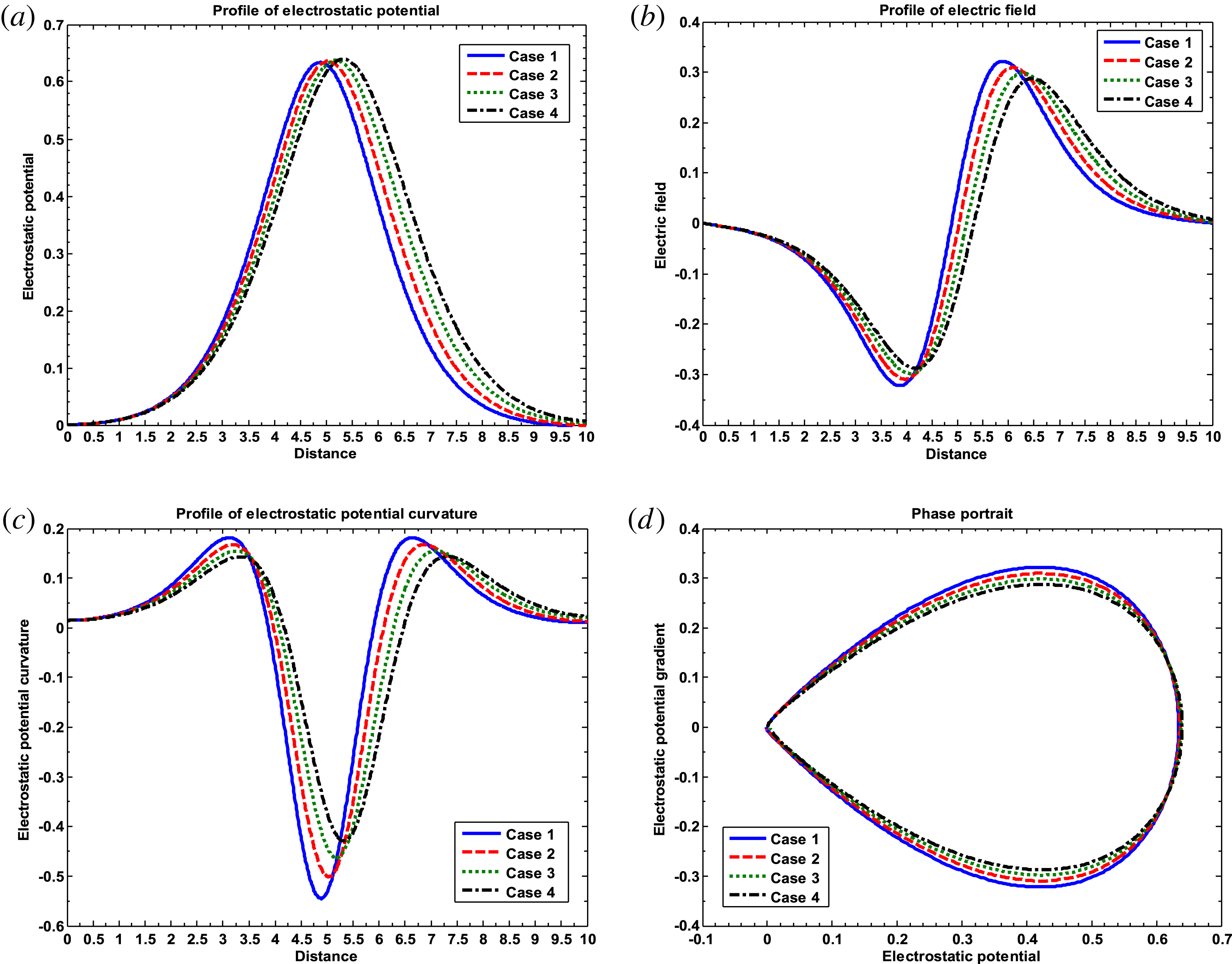
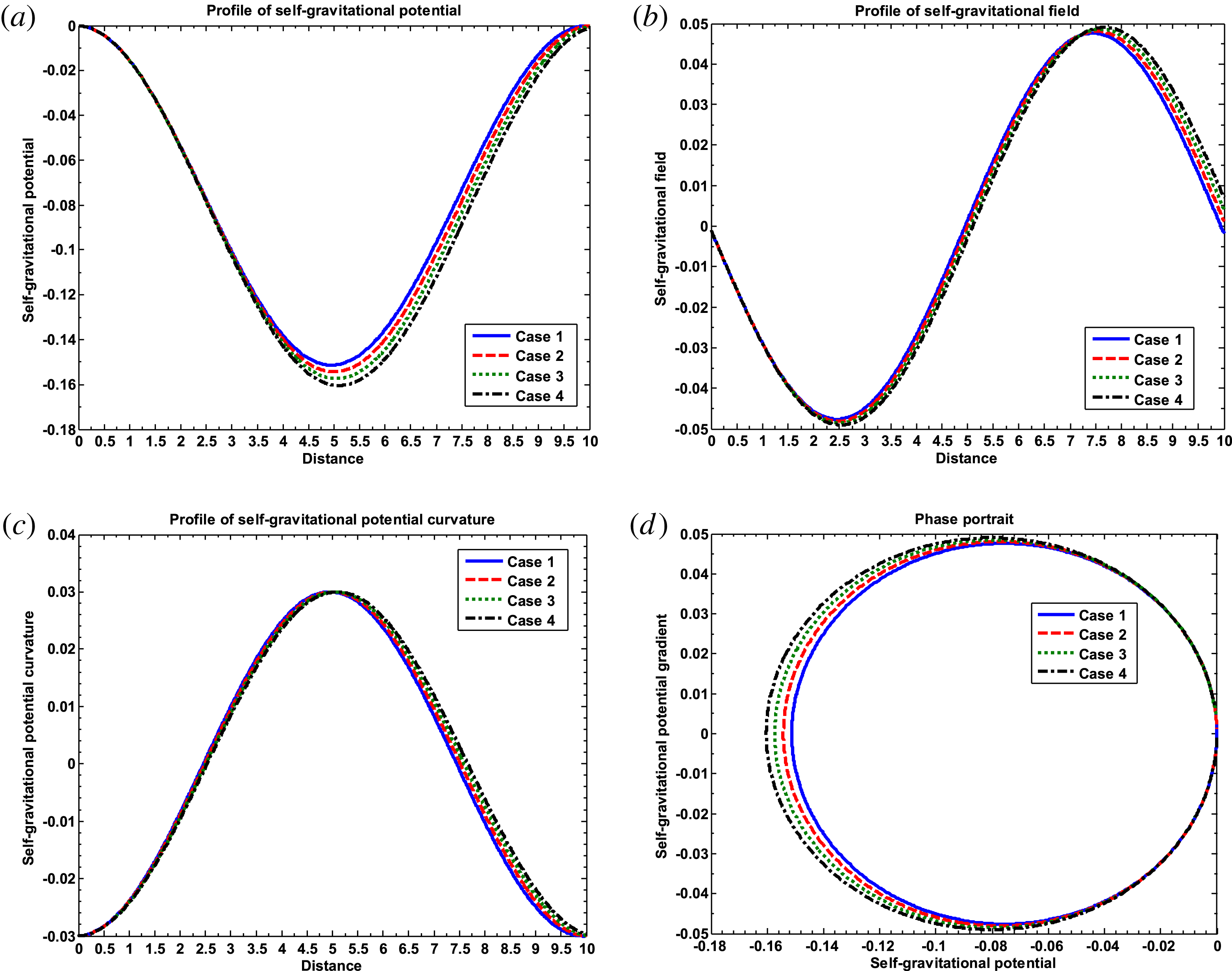
Spatial profile of the lowest-order perturbed electrostatic (a) potential, (b) field, (c) potential curvature, and (d) phase portrait. Various lines correspond to Case (1): $m_{d}=1.07\times 10^{-12}$  kg (blue line), Case (2): $m_{d}=1.12\times 10^{-12}$  kg (red line), Case (3): $m_{d}=1.17\times 10^{-12}$  kg (green line) and Case (4): $m_{d}=1.22\times 10^{-12}$  kg (black line). Different input initial values used are $({\it\Phi})_{i}=1.00\times 10^{-3}$ , $({\it\Phi}_{{\it\rho}})_{i}=-1.00\times 10^{-4}$ and $({\it\Phi}_{{\it\rho}{\it\rho}})_{i}=1.50\times 10^{-2}$ . The other parameters kept fixed are $Z_{d}=100$ , $n_{eo}=2.43\times 10^{3}~\text{m}^{-3}$ , $n_{io}=1.00\times 10^{3}~\text{m}^{-3}$ , $n_{do}=5.00\times 10^{-1}~\text{m}^{-3}$ and ${\it\mu}=1.00$ .

1. (1) For $n_{eo}=2.43\times 10^{3}~\text{m}^{-3}$ , $2.53\times 10^{3}~\text{m}^{-3}$ , $2.63\times 10^{3}~\text{m}^{-3}$ , we obtain $A_{1}=4.85$ , 5.05, 5.25 and $A_{2}=6.12\times 10^{-1}$ , $5.88\times 10^{-1}$ , $5.65\times 10^{-1}$ ; respectively. Thus, as $n_{eo}$ increases, the nonlinear effect (via $A_{1}$ ) increases and the dispersive effect (via $A_{2}$ ) decreases; and vice versa.

2. (2) For $n_{io}=1.00\times 10^{3}~\text{m}^{-3}$ , $1.50\times 10^{3}~\text{m}^{-3}$ , $2.00\times 10^{3}~\text{m}^{-3}$ , one has $A_{1}=4.85$ , 3.23, 2.42 and $A_{2}=6.120\times 10^{-1}$ , $6.128\times 10^{-1}$ , $6.130\times 10^{-1}$ ; respectively. This shows that, when $n_{io}$ increases, $A_{1}$ decreases and $A_{2}$ increases; and vice versa.

3. (3) For $n_{do}=5.00\times 10^{-1}~\text{m}^{-3}$ , $6.00\times 10^{-1}~\text{m}^{-3}$ , $7.00\times 10^{-1}~\text{m}^{-3}$ , one gets $A_{1}=4.85$ and $A_{2}=6.12\times 10^{-1}$ , $7.34\times 10^{-1}$ , $8.57\times 10^{-1}$ ; respectively. Thus, as $n_{do}$ increases, $A_{1}$ remains the same and $A_{2}$ increases; and vice versa.

4. (4) Further, it is found that there is no sensitive dependence of $A_{1}$ and $A_{2}$ on $Z_{d}$ .

5. (5) For ${\it\alpha}=6.40\times 10^{14}$ , $6.50\times 10^{14}$ , $6.60\times 10^{14}$ , one has $A_{1}=4.85$ and $A_{2}=6.12\times 10^{-1}$ , $6.23\times 10^{-1}$ , $6.35\times 10^{-1}$ ; respectively. Thus, as ${\it\alpha}$ increases, $A_{1}$ remains the same and $A_{2}$ increases; and vice versa.

6. (6) Lastly, for $T_{i}/T_{e}=1.00\times 10^{-3}$ , $5.00\times 10^{-3}$ , $1.00\times 10^{-2}$ , one has $A_{1}=4.85$ , 4.83, 4.80 and $A_{2}=6.12\times 10^{-1}$ , $6.06\times 10^{-1}$ , $5.99\times 10^{-1}$ ; respectively. Thus, as $T_{i}/T_{e}$ increases, both $A_{1}$ and $A_{2}$ decrease; and vice versa.

Likewise, a similar treatment by the same method of decoupling to (3.26), as shown in the appendix, yields the following KdV equation for the weakly nonlinear self-gravitational fluctuations (in terms of ${\it\Psi}_{1}$ ) on the Jeans scales of space and time,

where,

Analytically, again as in the case of electrostatic counterparts, it is evident from (3.31)–(3.32) that both the self-gravitational convective coefficient $B_{1}$ and self-gravitational dispersive coefficient $B_{2}$ sensitively depend on diverse plasma parameters. The quantifiable flavor of $B_{1}$ and $B_{2}$ in the normal cloud plasma conditions is tinted as in the next.

1. (1) For $n_{eo}=2.50\times 10^{3}~\text{m}^{-3}$ , $2.60\times 10^{3}~\text{m}^{-3}$ , $2.70\times 10^{3}~\text{m}^{-3}$ , we obtain $B_{1}=3.20\times 10^{-3}$ , $3.30\times 10^{-3}$ , $3.40\times 10^{-3}$ and $B_{2}=-2.52$ , $-2.42$ , $-2.33$ ; respectively. Thus, as $n_{eo}$ increases, $B_{1}$ increases and $B_{2}$ decreases in magnitude; and vice versa.

2. (2) For $n_{io}=1.00\times 10^{3}~\text{m}^{-3}$ , $1.50\times 10^{3}~\text{m}^{-3}$ , $2.00\times 10^{3}~\text{m}^{-3}$ , one has $B_{1}=3.20\times 10^{-3}$ , $2.10\times 10^{-3}$ , $1.60\times 10^{-3}$ and $B_{2}=-2.52$ , $-3.78$ , $-5.04$ ; respectively. Thus, as $n_{io}$ increases, $B_{1}$ decreases and $B_{2}$ increases in magnitude; and vice versa.

3. (3) For $Z_{d}=100$ , 105, 110, one has $B_{1}=3.20\times 10^{-3}$ , $3.00\times 10^{-3}$ , $2.90\times 10^{-3}$ and $B_{2}=-2.52$ , $-2.64$ , $-2.77$ ; respectively. Thus, as $Z_{d}$ increases, $B_{1}$ decreases and $B_{2}$ increases in magnitude; and vice versa.

4. (4) Lastly, there is no sensitive dependence of $B_{1}$ and $B_{2}$ on $n_{do}$ , ${\it\alpha}$ , $T_{i}/T_{e}$ and $T_{d}/T_{e}$ .

To see the time-stationary dynamics of the weakly nonlinear gravito-electrostatic eigenmodes, (3.27) and (3.30) are transformed into ordinary differential equations (ODEs) by the Galilean comoving frame transformation, ${\it\rho}=X-T$ . Thus, (3.27) and (3.30) in time-stationary form are respectively given by

Clearly, (3.33) and (3.34) together constitute a unique steady-state pair of decoupled KdV equations paving the way for solitary pattern existence in the new spatial coordinate system (defined by ${\it\rho}$ ). It may be noted that there is no self-consistent source, nor any sink in the KdV system, unlike previously reported results on the nonlinear evolution of electrostatic dust-acoustic waves in a uniform gravitating dusty plasma configuration with all the constituents politropically treated alike (Verheest & Shukla Reference Verheest and Shukla1997; Verheest Reference Verheest2000). In the latter case, the dust-acoustic mode evolution has been found to be governed by the extended KdV equation having a self-consistent non-local linear integral sink term arising due to the self-gravitational force field acting on the gravitating massive dust grains.

The steady-state analytical solution of (3.33), obtained by applying the technique of approximate analytical integration, as used by other authors in the past (Mamun & Shukla Reference Mamun and Shukla2002; Shukla & Mamun Reference Shukla and Mamun2003), can explicitly be written as

where, $({\it\Phi}_{1})_{m}=3/A_{1}\approx 6.18\times 10^{-1}$ is the amplitude of the electrostatic soliton with average width ${\it\Delta}_{ES}=\sqrt{4A_{2}}\approx 1.56$ . The value of the convective coefficient $A_{1}=4.85$ and dispersive coefficient $A_{2}=6.12\times 10^{-1}$ are analytically obtained by using the same plasma parameter values as in figure 1. It is seen that the analytically calculated solitary wave amplitude $({\it\Phi}_{1})_{m}$ exactly matches that obtained by exact numerical integration (figures 1 a–2 a).

Figure 2.

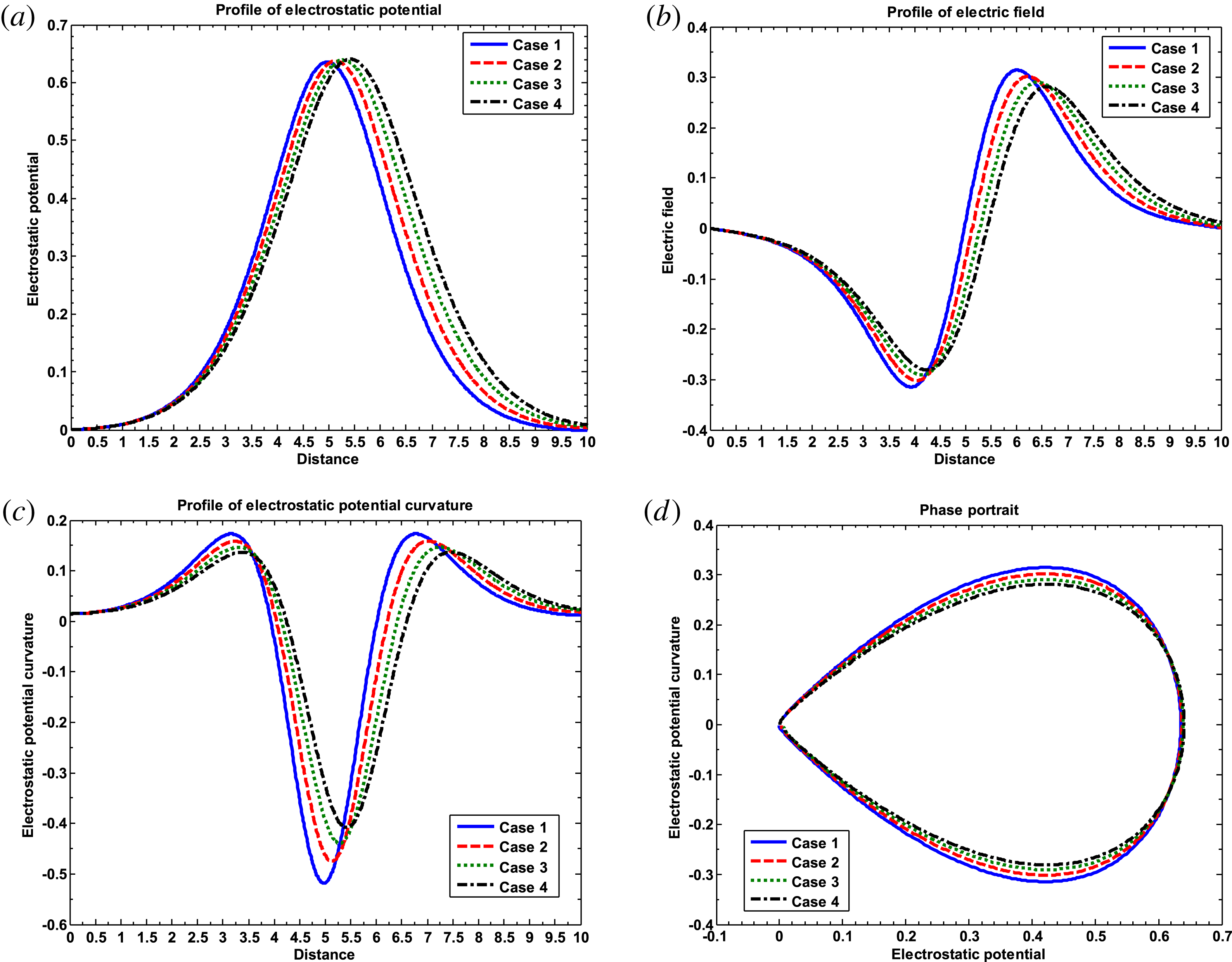
Same as figure 1. Various lines now correspond to Case (1): $n_{do}=5.00\times 10^{-1}~\text{m}^{-3}$ (blue line), Case (2): $n_{do}=5.50\times 10^{-1}~\text{m}^{-3}$ (red line), Case (3): $n_{do}=6.00\times 10^{-1}~\text{m}^{-3}$ (green line) and Case (4): $n_{do}=6.50\times 10^{-1}~\text{m}^{-3}$ (black line).

Again, similar to the electrostatic counterpart, the approximate analytical solution of (3.34) can be written as,

where, $({\it\Psi}_{1})_{m}=3/B_{1}\approx 9.37\times 10^{3}$ is the amplitude of the self-gravitational soliton with average width ${\it\Delta}_{GS}=\sqrt{4|B_{2}|}\approx 3.17$ . The value of the convective coefficient $B_{1}=3.20\times 10^{-3}$ and dispersive coefficient $B_{2}=-2.52$ are analytically obtained by using the same plasma parameter values as are used in figure 4. The analytically (with the approximation of asymptotic behaviour) calculated solitary wave amplitude $({\it\Psi}_{1})_{m}$ shows a minor deviation from that obtained by numerical (with no approximation, exact) analysis (figures 4 a–5 a). This shows that there is always some deviation in fluctuation patterns because of the approximate analytical integration in contrast with exact numerical integration (figures 4 a–5 a).

3.3 Application of the Sagdeev pseudo-potential method

In this section we study the properties of strongly nonlinear (arbitrary amplitude) gravito-electrostatic waves by applying the Sagdeev pseudo-potential approach (Sagdeev Reference Sagdeev and Leontovich1966). Here, we introduce a Galilean frame, ${\it\rho}={\it\xi}-{\it\mu}{\it\tau}$ , where ${\it\mu}$ is the reference frame velocity (normalized by $C_{SS}$ ), to obtain the time-stationary construct of the governing equations. Applying the appropriate boundary conditions, such as $M_{d}\rightarrow 0$ , $N_{i}\rightarrow 1$ , ${\it\Phi}\rightarrow 0$ and ${\it\Psi}\rightarrow 0$ at ${\it\rho}\rightarrow \pm \infty$ in the stationary frame, (3.2) and (3.4)–(3.6) are transformed as,

Now, substituting for $N_{e}$ , $N_{i}$ and $N_{d}$ from (3.1), (3.37) and (3.38) in (3.5) and (3.6), one obtains the following second-order differential equations,

and

where,

Here, ${\it\eta}_{i}=({\it\rho}_{i}-{\it\rho}_{io})$ and ${\it\eta}_{d}=({\it\rho}_{d}-{\it\rho}_{do})$ are defined as the average transit scale lengths of the ions and the grains, respectively, which typically are ${\sim}{\it\lambda}_{J}$ .

In the electrostatic case, multiplying both sides of (3.39) by $\partial {\it\Phi}/\partial {\it\rho}$ and integrating once under the appropriate boundary conditions, such as ${\it\Phi}\rightarrow 0$ and $\partial {\it\Phi}/\partial {\it\rho}\rightarrow 0$ at ${\it\rho}\rightarrow \pm \infty$ for the localized structure of the disturbance, we obtain the electrostatic energy integral (Sagdeev Reference Sagdeev and Leontovich1966; Rao, Shukla & Yu Reference Rao, Shukla and Yu1990; Mace & Hellberg Reference Mace and Hellberg1993; Mamun, Cairns & Shukla Reference Mamun, Cairns and Shukla1996; Shukla & Mamun Reference Shukla and Mamun2003; Lakhina et al. Reference Lakhina, Singh and Kakad2010; Maharaj et al. Reference Maharaj, Bharuthram, Singh and Lakhina2015) as follows,

which describes the energy conservation principle of the electrostatic fluctuation dynamics subjected to the Sagdeev pseudo-potential, $V_{E}({\it\Phi},{\it\Psi})$ , given by

The approximate analytical solution of (3.43) in explicit form can be obtained by direct integration, with the inserted integration constant $K_{E}$ , as shown below,

where,

It is discernible that the mathematical construct of (3.45) is highly complicated, convoluted and nonlinear in nature. So derivation of analytical (approximate) solutions is skipped here and the numerical (exact) results are presented later. Now, after differentiating (3.44) successively with respect to ${\it\Phi}$ , one finds the following,

We now carry out prerequisite analytical tests to check the conditions for the existence of solitary structures and their qualitative properties governed by (3.43). It is found that (3.44), (3.48)–(3.50) under cold plasma conditions, $T_{s}/T_{e}\sim 0$ (Shukla Reference Shukla2002), satisfy the following extreme conditions meant for the existence of electrostatic compressive soliton-like structures (Mamun et al. Reference Mamun, Cairns and Shukla1996; Lakhina et al. Reference Lakhina, Singh and Kakad2010; Maharaj et al. Reference Maharaj, Bharuthram, Singh and Lakhina2015) as follows,

In (3.51), it is seen that $\partial ^{3}V_{E}({\it\Phi},{\it\Psi})/\partial {\it\Phi}^{3}>0$ at ${\it\Phi}=0$ , ${\it\Psi}=0$ , which is the condition for existence of compressive solitonic structures (Maharaj et al. Reference Maharaj, Bharuthram, Singh and Lakhina2015). So analytical scrutiny shows the evolutionary possibility for compressive solitary patterns.

In a similar manner, for the self-gravitational counterparts, we multiply (3.40) by $\partial {\it\Psi}/\partial {\it\rho}$ and integrate once with appropriate boundary conditions, such as ${\it\Psi}\rightarrow 0$ and $\partial {\it\Psi}/\partial {\it\rho}\rightarrow 0$ at ${\it\rho}\rightarrow \pm \infty$ , for a localized disturbance to survive. Thus, the self-gravitational energy-integral equation is systematically obtained as follows,

which depicts the energy conservation law of the self-gravitational fluctuation dynamics subjected to the self-gravitational Sagdeev pseudo-potential $V_{G}({\it\Phi},{\it\Psi})$ pronounced as,

Now, the approximate analytical solution of (3.52) can also be derived by direct integration with integration constant $K_{G}$ as in the following,

As in the case of electrostatic formalism, here too, the mathematical structure of (3.54) is highly complicated, intricate and nonlinear in shape, and is therefore skipped here and the exact numerical solutions are presented later. Now, differentiating (3.53) successively with respect to ${\it\Psi}$ , one obtains

It is analytically verified that (3.53), (3.55)–(3.57) satisfy the following conditions predicting the dynamical evolution of possible self-gravitational rarefactive soliton-like patterns (Mamun et al. Reference Mamun, Cairns and Shukla1996; Lakhina et al. Reference Lakhina, Singh and Kakad2010; Maharaj et al. Reference Maharaj, Bharuthram, Singh and Lakhina2015) as follows,

In (3.58), it is found that $\partial ^{3}V_{G}({\it\Phi},{\it\Psi})/\partial {\it\Psi}^{3}<0$ at ${\it\Phi}=0$ , ${\it\Psi}=0$ , which is the condition for the existence of rarefactive solitonic structures (Maharaj et al. Reference Maharaj, Bharuthram, Singh and Lakhina2015). As with electrostatic fluctuations, an analytical inspection of the existential conditions for the self-gravitational fluctuations shows the growth possibility for rarefactive soliton-like structures.

It may be seen that the conditions for the existence of electrostatic compressive soliton-like structures are $\partial ^{3}V_{E}({\it\Phi},{\it\Psi})/\partial {\it\Phi}^{3}>0,\partial ^{3}V_{G}({\it\Phi},{\it\Psi})/\partial {\it\Psi}^{3}>0$ at ${\it\Phi}=0$ , ${\it\Psi}=0$ , whereas, for gravitational rarefactive soliton-like patterns, the same are $\partial ^{3}V_{E}({\it\Phi},{\it\Psi})/\partial {\it\Phi}^{3}<0,\partial ^{3}V_{G}({\it\Phi},{\it\Psi})/\partial {\it\Psi}^{3}<0$ (Maharaj et al. Reference Maharaj, Bharuthram, Singh and Lakhina2015). For exact and precise characterization of the supported wave spectrum with these basic inputs kept in mind, (3.43) and (3.52) are numerically integrated by the fourth-order Runge–Kutta (RK-IV) method as discussed in the next section.

4.1 Weakly nonlinear fluctuations

The obtained profiles of the weak fluctuations (both spatial, (3.33); and spatio-temporal, (3.27)) with a suitably wide range of judicious plasma parameter values (Pandey & Dwivedi Reference Pandey and Dwivedi1996; Pandey et al. Reference Pandey, Vranjes, Poedts and Shukla2002; Shukla & Stenflo Reference Shukla and Stenflo2006) are discussed below.

Figure 1 presents the spatial profile of the lowest-order perturbed electrostatic (a) potential, (b) field, (c) potential curvature and (d) phase portrait. Various lines correspond to Case (1): $m_{d}=1.07\times 10^{-12}$  kg (blue line), Case (2): $m_{d}=1.12\times 10^{-12}$  kg (red line), Case (3): $m_{d}=1.17\times 10^{-12}$  kg (green line) and Case (4): $m_{d}=1.22\times 10^{-12}$  kg (black line). Different input initial values used are $({\it\Phi})_{i}=1.00\times 10^{-3}$ , $({\it\Phi}_{{\it\rho}})_{i}=-1.00\times 10^{-4}$ and $({\it\Phi}_{{\it\rho}{\it\rho}})_{i}=1.50\times 10^{-2}$ . The other parameters kept fixed are $Z_{d}=100$ , $n_{eo}=2.43\times 10^{3}~\text{m}^{-3}$ , $n_{io}=1.00\times 10^{3}~\text{m}^{-3}$ , $n_{do}=5.00\times 10^{-1}~\text{m}^{-3}$ and ${\it\mu}=1.00$ . The potential fluctuations (figure 1 a) show compressive soliton-like eigenmodes, which are in qualitatively good correspondence with those as obtained by others in different situations (Mamun et al. Reference Mamun, Cairns and Shukla1996; Verheest & Shukla Reference Verheest and Shukla1997; Ergun et al. Reference Ergun, Carlson, McFadden, Mozer, Delory, Peria, Chaston, Ternerin, Roth and Muschietti1998; Mamun Reference Mamun1999; Omur et al. Reference Omur, Kojima, Miki, Mukai, Matsumoto and Anderson1999; Burman & Chowdhury Reference Burman and Chowdhury2002; Shukla & Mamun Reference Shukla and Mamun2003). We see that when $m_{d}$ increases, the soliton peak slightly shifts away from that at ${\it\rho}=5{\it\lambda}_{J}$ (figure 1 a). This shows that the fluctuations propagate away from the centre outwards with increasing $m_{d}$ . This physically means that increasing $m_{d}$ upturns dispersive effects sourced by the self-gravitational field (Newton) and space-charge polarization (Poisson). Subsequently, the combined effects of gravito-electrostatic coupling result in soliton broadening. The corresponding fields (figure 1 b) and curvature fluctuation (figure 1 c) profile show a mixture of rarefactive and compressive solitons; and bell-shaped soliton-like structures, respectively. Lastly, figure 1(d) shows the phase portraits in the phase space spanned by ${\it\Phi}_{1}$ and ${\it\Phi}_{1{\it\rho}}$ , which gives a parametric representation of the geometrical trajectories for the global behaviour of the local fluctuations.

Figure 2 portrays the same as figure 1. Various lines now stand for Case (1): $n_{do}=5.00\times 10^{-1}~\text{m}^{-3}$ (blue line), Case (2): $n_{do}=5.50\times 10^{-1}~\text{m}^{-3}$ (red line), Case (3): $n_{do}=6.00\times 10^{-1}~\text{m}^{-3}$ (green line) and Case (4): $n_{do}=6.50\times 10^{-1}~\text{m}^{-3}$ (black line). All the profiles show almost similar characteristics as in figure 1.

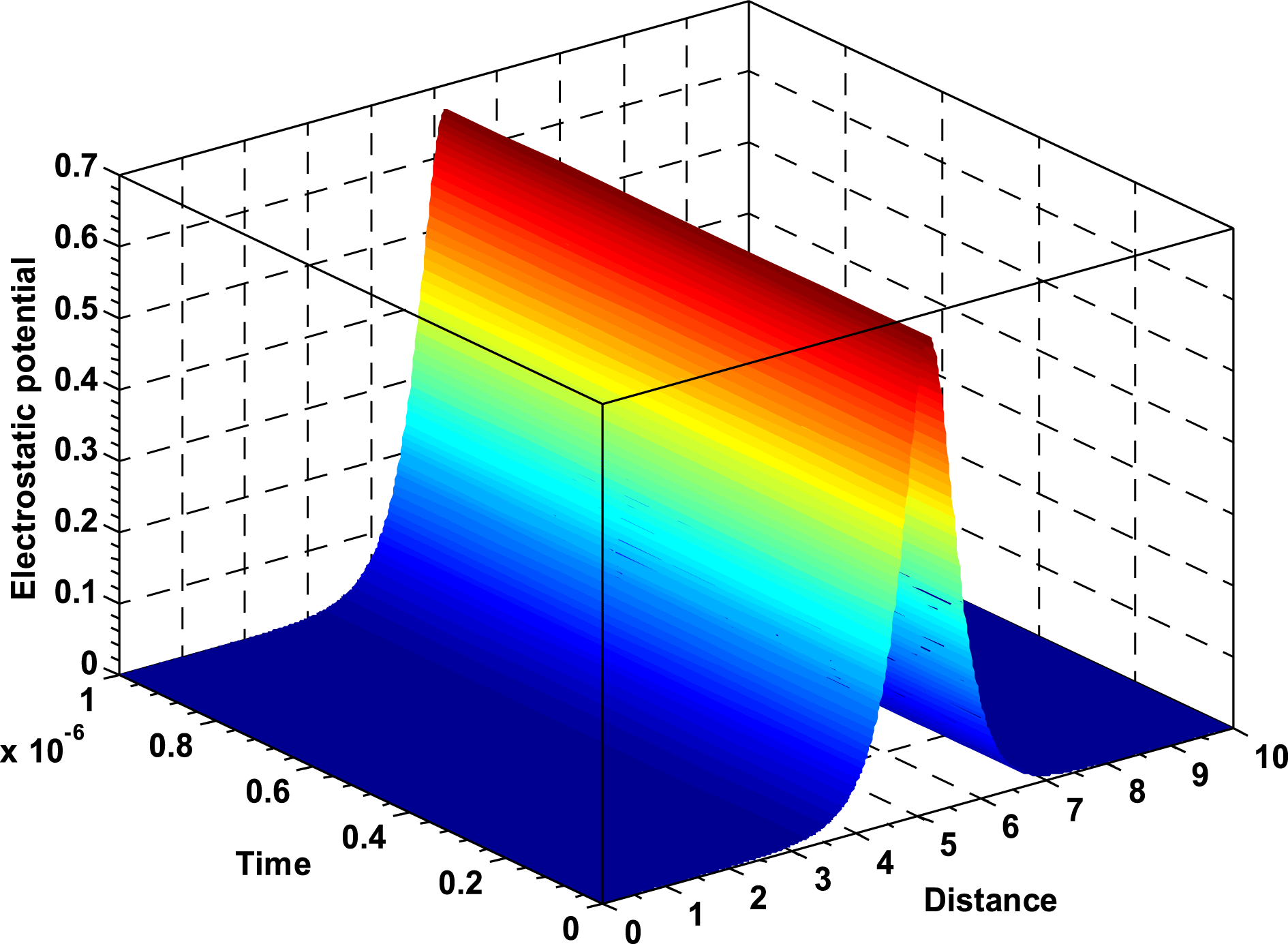
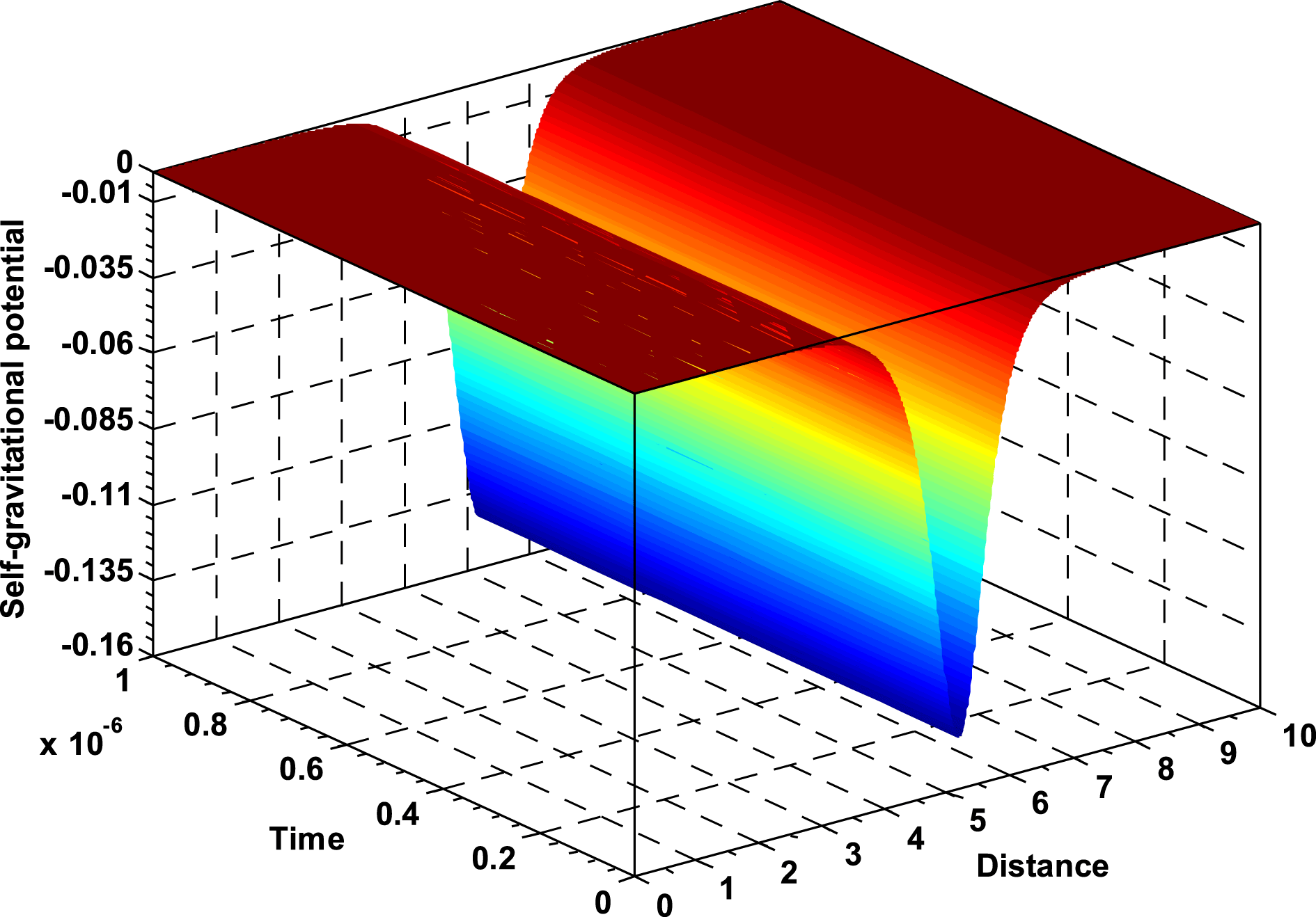
For the spatio-temporal evolution, (3.27) is integrated by the FD under suitable boundary conditions, as discussed above. Figure 3 depicts the perturbed potential evolving in astrophysical space and time under the same conditions as figure 1, but now with the numerically fitted (via trial-and-error, but soliton-like) initial value, ${\it\Phi}_{1,i}(X,0)=0.66\sec h(X^{1.4}-10)$ . Though it is well known that the soliton is of the $\sec h^{2}$ -form, spatio-temporal evolution is found to be possible only for the $\sec h$ -input, also termed the similariton, resembling the Gaussian soliton. It is worth mentioning that the $\sec h$ -solitary patterns have widely been studied by many authors in the past for different nonlinear systems (Lakshmanan & Rajasekar Reference Lakshmanan and Rajasekar2003). The boundary conditions applied here are: (i) densities and dust charge at infinity are asymptotically zero, (ii) velocities at the centre are zero and (iii) potentials at the centre and asymptotically at infinity are zero. The snapshot of figure 3 is the same in magnitude and structure as in figures 1 and 2. It reflects the basic normal feature of the solitary structures as being temporally stable ones.

Figure 3.

Spatio-temporal profile of the lowest-order perturbed electrostatic potential under the same condition as figure 1. The boundary conditions and input initial values used are presented in the text.

The physical strength of the potential fluctuations (figures 1 a–2 a) for average normalized value ${\it\Phi}_{1}\sim 6.25\times 10^{-1}$ is estimated as, ${\it\Phi}_{phys}\sim {\it\epsilon}(T_{e}{\it\Phi}_{1}/e)\sim 10^{-3}$  V, in the HII region with ${\it\epsilon}=10^{-2}$ (Pandey et al. Reference Pandey, Vranjes, Poedts and Shukla2002; Shukla & Stenflo Reference Shukla and Stenflo2006) and $T_{e}=10^{4}$  K. The wave amplitude is maximum at ${\it\rho}=5{\it\lambda}_{J}$ . The field fluctuations (figures 1 b–2 b) evolve with amplitudes having average normalized value ${\sim}4\times 10^{-1}$ , which is physically calculated as, $E_{phys}\sim {\it\epsilon}(T_{P}E_{e1}/e{\it\lambda}_{J})\sim 4.00\times 10^{-11}~\text{V}~\text{m}^{-1}$ . The curvature profiles (figures 1 c–2 c) exhibit bell-shaped solitary eigenmodes. The degree of deviation from the cloud quasi-neutrality is not uniform in the presence of the gravitating ions; it shows noticeable variation for $3{\it\lambda}_{J}<{\it\rho}<7.5{\it\lambda}_{J}$ with the maximum at ${\it\rho}=5{\it\lambda}_{J}\sim 5\times 10^{8}$  m. The average curvature fluctuation strength is calculated as, $(\partial _{xx}{\it\Phi})_{phys}\sim {\it\epsilon}(T_{p}\partial _{{\it\rho}{\it\rho}}{\it\Phi}_{1}/e{\it\lambda}_{J}^{2})\sim 2.00\times 10^{-19}~\text{Vm}^{-2}$ , which is very small ( ${\sim}$ 0). This signifies that the cloud quasi-neutrality is not affected appreciably due to the considered weakly nonlinear ( ${<}$ 3rd order) perturbation.

Figure 4.

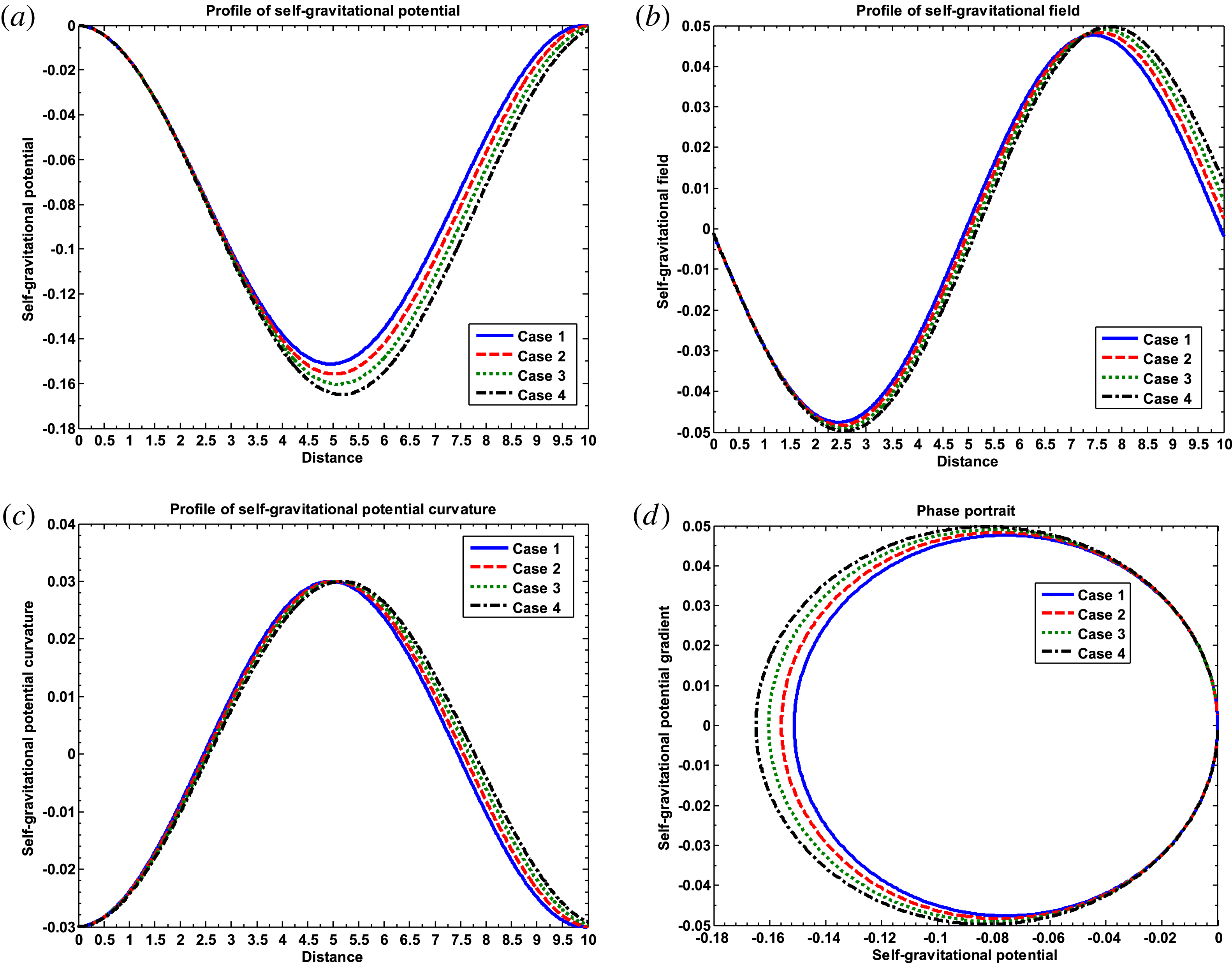
Spatial profile of the lowest-order perturbed self-gravitational (a) potential, (b) field, (c) potential curvature and (d) phase portrait. Various lines correspond to Case (1): $n_{io}=1.00\times 10^{3}~\text{m}^{-3}$ (blue line), Case (2): $n_{io}=1.03\times 10^{3}~\text{m}^{-3}$ (red line), Case (3): $n_{io}=1.06\times 10^{3}~\text{m}^{-3}$ (green line) and Case (4): $n_{io}=1.09\times 10^{3}~\text{m}^{-3}$ (black line). Different input initial values used are $({\it\Psi})_{i}=-1.00\times 10^{-4}$ , $({\it\Psi}_{{\it\rho}})_{i}=-1.00\times 10^{-3}$ and $({\it\Psi}_{{\it\rho}{\it\rho}})_{i}=-3.00\times 10^{-2}$ . The other parameters kept fixed are $Z_{d}=100$ , ${\it\mu}=0.06$ , $n_{eo}=2.50\times 10^{3}~\text{m}^{-3}$ , $n_{do}=1.00\times 10^{-1}~\text{m}^{-3}$ and $m_{d}=1.07\times 10^{-12}$  kg.

Let us now likewise describe the steady-state evolution of the self-gravitational fluctuation dynamics (governed by (3.34)). The resulting profiles are shown in figures 4–6. Figure 4 graphically gives the spatial profiles of the lowest-order perturbed self-gravitational (a) potential, (b) field, (c) potential curvature and (d) phase portrait. Various lines correspond to Case (1): $n_{io}=1.00\times 10^{3}~\text{m}^{-3}$ (blue line), Case (2): $n_{io}=1.03\times 10^{3}~\text{m}^{-3}$ (red line), Case (3): $n_{io}=1.06\times 10^{3}~\text{m}^{-3}$ (green line) and Case (4): $n_{io}=1.09\times 10^{3}~\text{m}^{-3}$ (black line). Different input initial values used are $({\it\Psi})_{i}=-1.00\times 10^{-4}$ , $({\it\Psi}_{{\it\rho}})_{i}=-1.00\times 10^{-3}$ and $({\it\Psi}_{{\it\rho}{\it\rho}})_{i}=-3.00\times 10^{-2}$ . The other parameters kept fixed are $Z_{d}=100$ , ${\it\mu}=0.06$ , $n_{eo}=2.50\times 10^{3}~\text{m}^{-3}$ , $n_{do}=1.00\times 10^{-1}~\text{m}^{-3}$ and $m_{d}=1.07\times 10^{-12}$  kg. The potential fluctuations evolve as bell-shaped soliton-like structures (figure 4 a), the amplitude of which increase with an increase in $n_{io}$ . As $n_{io}$ increases, the self-gravitational effects increase in the presence of the gravitating ions. As a consequence, the self-gravitational fluctuation increases. It provides strong evidence in support of the fact that the ion inertia makes an effective contribution to the propagation and excitation of eigenmodes. The corresponding field (figure 4 b) and curvature (figure 4 c) fluctuations evolve as hybridized mixtures of rarefactive and compressive soliton-like, and compressive soliton-like, structures, respectively. The phase portraits (figure 4 d) give the geometrical trajectories of the inertial species in the phase plane of ${\it\Psi}_{1}$ and ${\it\Psi}_{1{\it\rho}}$ . The trajectories show closed structures as a confirmation of the conservative system. Similarly, figure 5 gives the same as figure 4. Various lines are Case (1): $Z_{d}=100$ (blue line), Case (2): $Z_{d}=102$ (red line), Case (3): $Z_{d}=104$ (green line) and Case (4): $Z_{d}=106$ (black line). It is further seen that the spectral pattern and nature of figure 5 are almost similar to those of figure 4.

Figure 5.

Same as figure 4. Various lines now correspond to Case (1): $Z_{d}=100$ (blue line), Case (2): $Z_{d}=102$ (red line), Case (3): $Z_{d}=104$ (green line) and Case (4): $Z_{d}=106$ (black line).

Figure 6.

Spatio-temporal profile of the lowest-order perturbed self-gravitational potential under the same conditions as figure 4. The boundary conditions and input initial values used are presented in the text.

To obtain the 3-D spatio-temporal profile, (3.30) is numerically integrated as in the electrostatic case. The subsequent fluctuations evolve as shown in figure 6. The conditions are the same as figure 4, but with initial potential value, ${\it\Psi}_{1,i}(X,0)=0.14\sec h(X^{1.4}-10)$ . The magnitude and structure are the same as those of the time-stationary ones (figures 4 and 5).

The physical strength of the fluctuations for ${\it\Psi}_{1}\sim |1.6\times 10^{-1}|$ is estimated as, $|{\it\Psi}_{phys}|\sim {\it\epsilon}(C_{SS}^{2}{\it\Psi}_{1})\sim 2.24\times 10^{-11}~\text{J}~\text{kg}^{-1}$ , in the HII region, with ${\it\epsilon}=10^{-2}$ (Pandey et al. Reference Pandey, Vranjes, Poedts and Shukla2002; Shukla & Stenflo Reference Shukla and Stenflo2006) and $C_{SS}^{2}\sim 1.4\times 10^{-7}~\text{J}~\text{kg}^{-1}$ . The fluctuation strength peaks at ${\it\rho}=5{\it\lambda}_{J}\sim 5\times 10^{8}$  m. The field fluctuations (figures 4 b–5 b) evolve as hybrids of rarefactive and compressive solitonic patterns with average amplitude, $|E_{gphys}|\sim {\it\epsilon}(E_{g1}C_{SS}^{2}/{\it\lambda}_{J})\sim 7.00\times 10^{-19}~\text{J}~\text{kg}^{-1}~\text{m}^{-1}$ . The curvatures (figures 4 c–5 c) exhibit compressive solitary anatomical structures with average strength estimated as, $(\partial _{xx}{\it\Psi})_{phys}\sim {\it\epsilon}(\partial _{{\it\rho}{\it\rho}}{\it\Psi}_{1}C_{SS}^{2}/{\it\lambda}_{J}^{2})\sim 4.20\times 10^{-28}~\text{J}~\text{kg}^{-1}~\text{m}^{-2}$ , which is very small ( ${\sim}$ 0) owing to weak nonlinearly ( ${<}$ 3rd order) taken into account. Thus, the cloud inertial mass neutrality, although the active ion-inertial dynamics is taken into account, is not appreciably affected.

In comparison, we see that the strength of the self-gravitational fluctuations is weaker than for the electrostatic counterparts ( ${\it\Phi}_{1}/{\it\Psi}_{1}\approx 3.8$ ). The phase portraits of both the Coulombic (figures 1 d–2 d) and Newtonian (figures 4 d–5 d) species reveal a conservative dynamical system via closed-form structures. For increasing (decreasing) different plasma parameters, the trajectories overlap over one another at the potential value corresponding to that near the cloud centre. Therefore, it is pertinent to add that the central portion of the cloud surrounds the most stable fixed point.

4.2 Strongly nonlinear fluctuations

We analyse and characterize the strongly nonlinear (arbitrary amplitude) gravito-electrostatic fluctuations by numerically solving (3.43) and (3.52). It is noticeable that, as per our analytic tests for existence criterion of the fully nonlinear eigenmodes already mentioned in the previous section, the electrostatic and self-gravitational fluctuations are ensured to evolve respectively as compressive and rarefactive soliton-like structures numerically as well. The detailed characteristic features are in order.

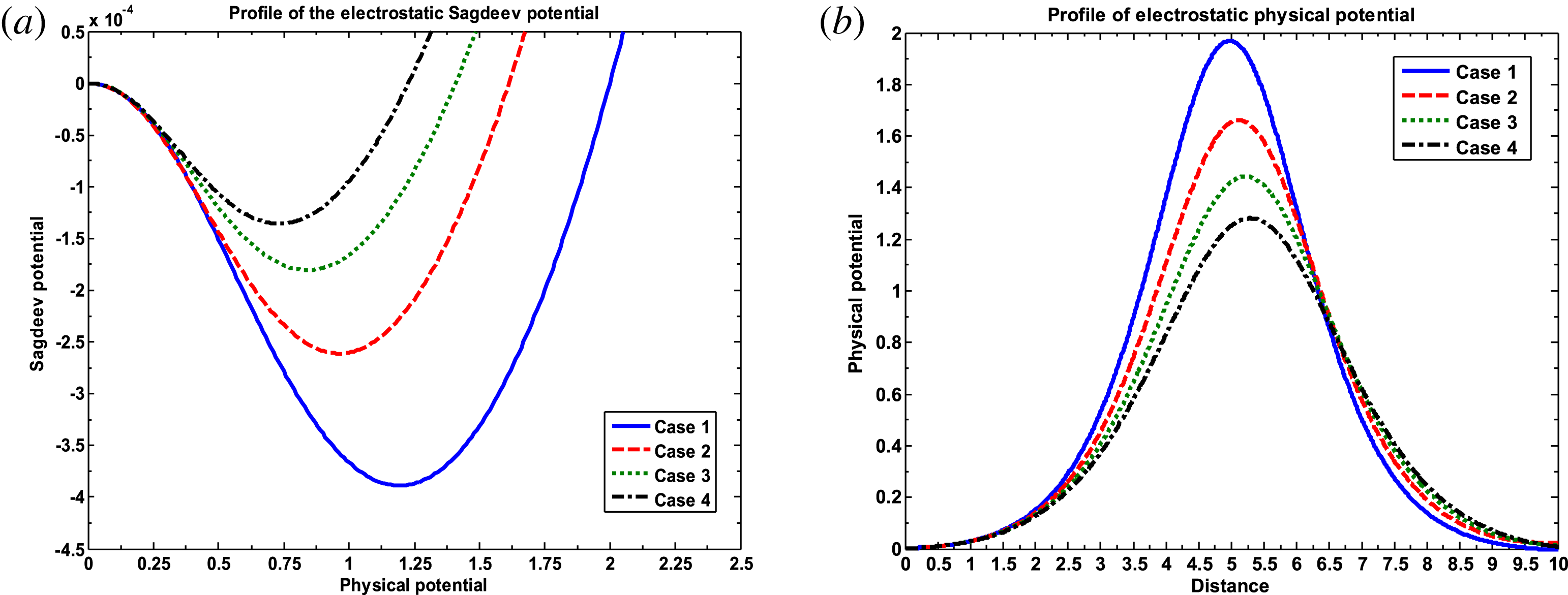
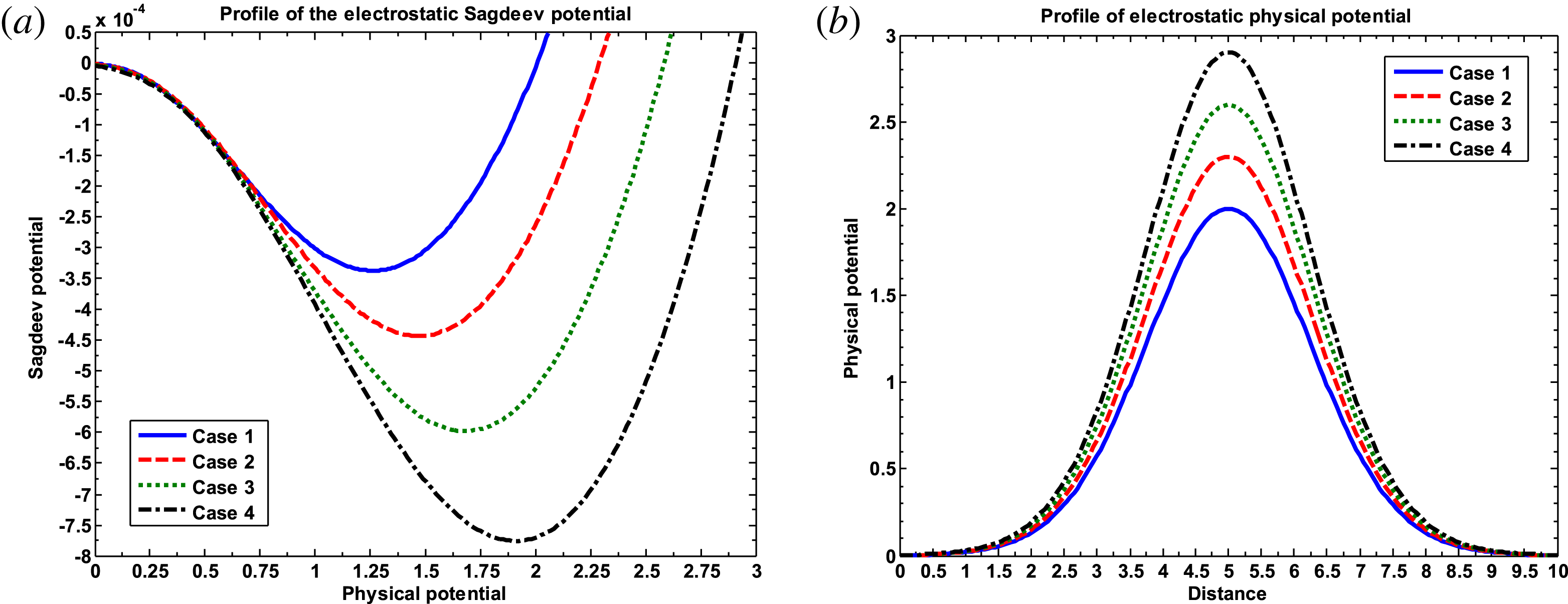
Figure 7 portrays the electro-dynamical evolution of the electrostatic (a) Sagdeev potential, and (b) physical potential. Various lines now represent Case (1): $n_{eo}=1.00\times 10^{7}~\text{m}^{-3}$ (blue line), Case (2): $n_{eo}=1.30\times 10^{7}~\text{m}^{-3}$ (red line), Case (3): $n_{eo}=1.60\times 10^{7}~\text{m}^{-3}$ (green line) and Case (4): $n_{eo}=1.90\times 10^{7}~\text{m}^{-3}$ (black line). The other parameters kept fixed are $Z_{d}=100$ , $n_{io}=7.00\times 10^{7}~\text{m}^{-3}$ , $n_{do}=5.00\times 10^{2}~\text{m}^{-3}$ , $m_{d}=4.00\times 10^{-12}$  kg, $F_{id}=1.00\times 10^{-4}$ and ${\it\mu}=1.00$ . The Sagdeev potential (figure 7 a) shows solitary eigenmodes, which satisfy all the analytical conditions pretested for the existence of solitary solutions. The physical potential (figure 7 b) evolves as compressive soliton-like structures corresponding to the Sagdeev potential (figure 7 a). In both the Sagdeev and physical potentials, the amplitude of the eigenmodes decreases with an increase in $n_{eo}$ . The basic physical insight underlying this is the same as discussed in the case of the weak fluctuations.

Figure 7.

Spatial profile of the electrostatic (a) Sagdeev potential and (b) physical potential. Various lines correspond to Case (1): $n_{eo}=1.00\times 10^{7}~\text{m}^{-3}$ (blue line), Case (2): $n_{eo}=1.30\times 10^{7}~\text{m}^{-3}$ (red line), Case (3): $n_{eo}=1.60\times 10^{7}~\text{m}^{-3}$ (green line) and Case (4): $n_{eo}=1.90\times 10^{7}~\text{m}^{-3}$ (black line). The initial value used here is $({\it\Phi})_{i}=1.20\times 10^{-9}$ . The other parameters kept fixed are $Z_{d}=100$ , $n_{io}=7.00\times 10^{7}~\text{m}^{-3}$ , $n_{do}=5.00\times 10^{2}~\text{m}^{-3}~m_{d}=4.00\times 10^{-12}$  kg,  $F_{id}=1.00\times 10^{-4}$ , and ${\it\mu}=15.0$ .

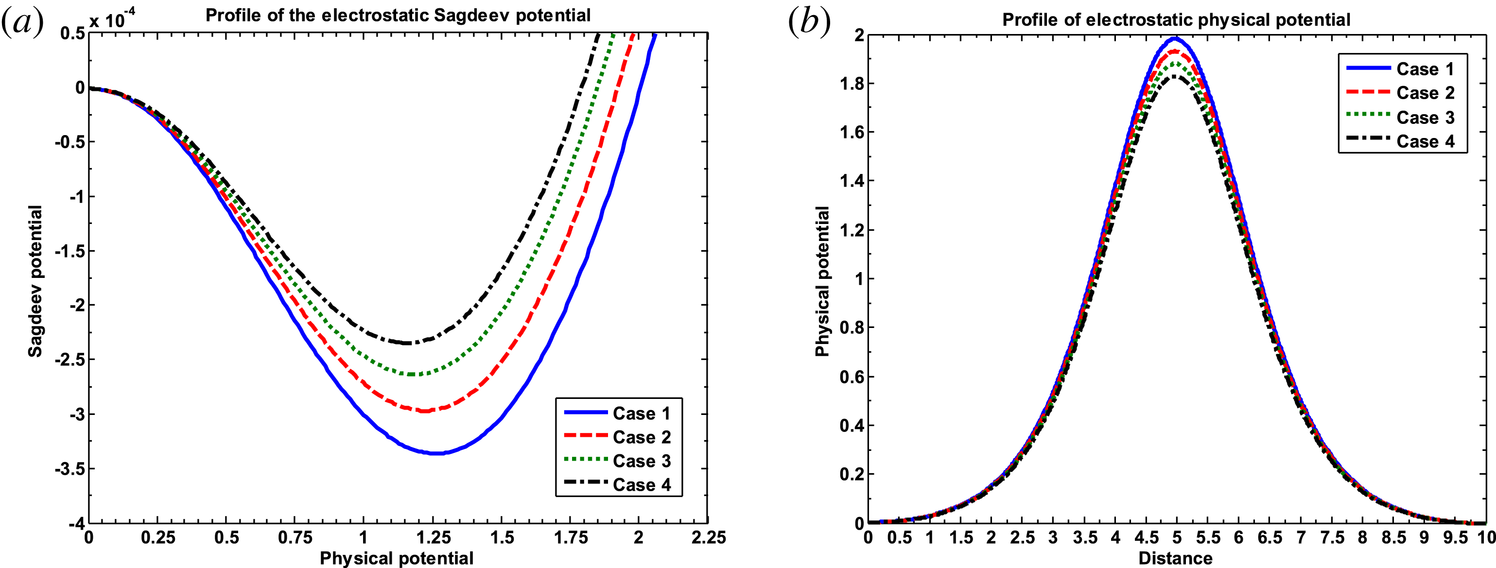
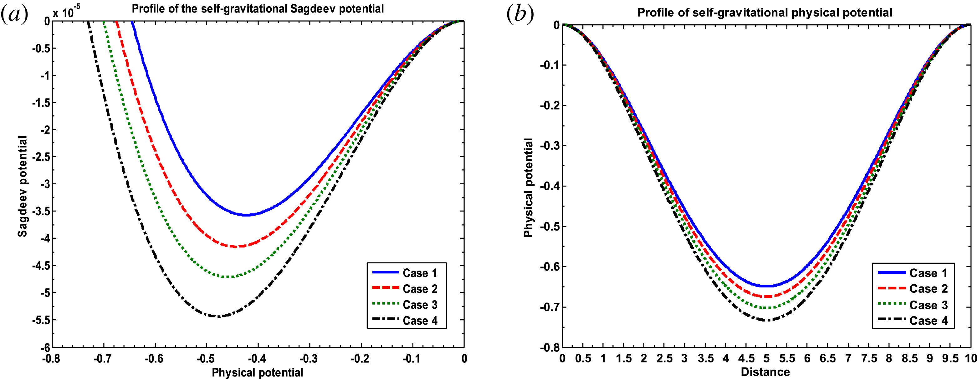
Analogously, figure 8 exhibits the same fluctuating patterns as figure 7. Various lines now stand for Case (1): $m_{d}=4.00\times 10^{-12}$  kg (blue line), Case (2): $m_{d}=4.30\times 10^{-12}$  kg (red line), Case (3): $m_{d}=4.60\times 10^{-12}$  kg (green line) and Case (4): $m_{d}=4.90\times 10^{-12}$  kg (black line). Here, as speculated in figure 1, we see similar features, but now in the fully nonlinear regime. It is interesting to note that for $10^{-13}<m_{d}<10^{-10}$  kg, the compressional solitary structures are supported in our cloud model.

Figure 8.

Same as figure 7. Various lines now correspond to Case (1): $m_{d}=4.00\times 10^{-12}$  kg (blue line), Case (2): $m_{d}=4.30\times 10^{-12}$ kg (red line), Case (3): $m_{d}=4.60\times 10^{-12}$  kg (green line) and Case (4): $m_{d}=4.90\times 10^{-12}$  kg (black line).

Furthermore, figure 9 presents the same as figure 7. Various lines now represent Case (1): $n_{do}=5.00\times 10^{2}~\text{m}^{-3}$ (blue line), Case (2): $n_{do}=7.00\times 10^{2}~\text{m}^{-3}$ (red line), Case (3) $n_{do}=9.00\times 10^{2}~\text{m}^{-3}$ (green line) and Case (4): $n_{do}=1.10\times 10^{3}~\text{m}^{-3}$ (black line). In figure 9, we find similar features as shown in figure 7.

Figure 9.

Same as figure 7. Various lines now correspond to Case (1): $n_{do}=5.00\times 10^{2}~\text{m}^{-3}$ (blue line), Case (2): $n_{do}=7.00\times 10^{2}~\text{m}^{-3}$ (red line), Case (3): $n_{do}=9.00\times 10^{2}~\text{m}^{-3}$ (green line) and Case (4): $n_{do}=1.10\times 10^{3}~\text{m}^{-3}$ (black line).

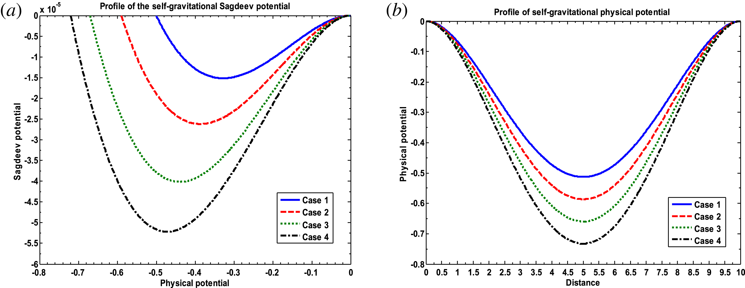
In a parallel manner, figure 10 presents evolutionary profiles of the self-gravitational (a) Sagdeev potential, and (b) physical potential. Various lines are now Case (1): $n_{io}=6.00\times 10^{4}~\text{m}^{-3}$ (blue line), Case (2): $n_{io}=6.30\times 10^{4}~\text{m}^{-3}$ (red line), Case (3): $n_{io}=6.60\times 10^{4}~\text{m}^{-3}$ (green line) and Case (4): $n_{io}=6.90\times 10^{4}~\text{m}^{-3}$ (black line). The other parameters kept fixed are $Z_{d}=110$ , $n_{do}=1.00\times 10^{1}~\text{m}^{-3}~m_{d}=4.00\times 10^{-12}$  kg, $F_{id}=1.00\times 10^{-4}$ and ${\it\mu}=1.00$ . Here, as already confirmed analytically before, it is found that the Sagdeev potential (figure 10 a) satisfies the requisite criterion, thereby allowing the real potential to evolve rarefactive solitary waves (figure 10 b) for $10^{4}<n_{io}<10^{6}~\text{m}^{-3}$ . The basic mechanism is the same as in figure 4.

Figure 10.

Spatial profile of the self-gravitational (a) Sagdeev potential and (b) physical potential. Various lines now correspond to Case (1): $n_{io}=6.00\times 10^{4}~\text{m}^{-3}$ (blue line), Case (2): $n_{io}=6.30\times 10^{4}~\text{m}^{-3}$ (red line), Case (3): $n_{io}=6.60\times 10^{3}~\text{m}^{-3}$ (green line) and Case (4): $n_{io}=6.90\times 10^{3}~\text{m}^{-3}$ (black line). The initial value used here is $({\it\Psi})_{i}=-1.00\times 10^{-9}$ . The other parameters kept fixed are $Z_{d}=110$ , $n_{do}=1.00\times 10^{1}~\text{m}^{-3}~m_{d}=4.00\times 10^{-12}$  kg,  $F_{id}=1.00\times 10^{-4}$ and ${\it\mu}=1.00$ .

Lastly, figure 11 gives the same as figure 10. Various lines now describe Case (1): $n_{do}=0.70\times 10^{1}~\text{m}^{-3}$ (blue line), Case (2): $n_{do}=0.80\times 10^{1}~\text{m}^{-3}$ (red line), Case (3): $n_{do}=0.90\times 10^{1}~\text{m}^{-3}$ (green line) and Case (4): $n_{do}=1.00\times 10^{1}~\text{m}^{-3}$ (black line). It is seen that the solitary amplitude increases with increasing $n_{do}$ in the range $10^{-1}<n_{do}<10^{3}~\text{m}^{-3}$ . The amplitude growth is attributable to the ion-inertial effects (figure 10) and the dust-inertial effects (figure 11) within the classical limit of the Newtonian dynamics.

Figure 11.

Same as figure 10. Various lines now correspond to Case (1): $n_{do}=0.70\times 10^{1}~\text{m}^{-3}$ (blue line), Case (2): $n_{do}=0.80\times 10^{1}~\text{m}^{-3}$ (red line), Case (3): $n_{do}=0.90\times 10^{1}~\text{m}^{-3}$ (green line) and Case (4): $n_{do}=1.00\times 10^{1}~\text{m}^{-3}$ (black line).

The physical strength of the strongly nonlinear electrostatic potential for the average normalized potential ${\it\Phi}_{N}\sim 2.00$ is calculated as, ${\it\Phi}_{p}\sim 2.00$  V, in the HII region with $T_{e}\sim 10^{4}$  K (Pandey et al. Reference Pandey, Vranjes, Poedts and Shukla2002; Shukla & Stenflo Reference Shukla and Stenflo2006). Similarly, the physical value of the self-gravitational potential is, ${\it\Psi}_{p}\sim 1.12\times 10^{-9}~\text{J}~\text{kg}^{-1}$ , for the average normalized potential, ${\it\Psi}_{N}\sim 8.00\times 10^{-1}$ . Thus, the electrostatic repulsive potential overcomes the self-gravitational attractive counterpart in both the regimes of weak nonlinearity ( ${\it\Phi}_{1}/{\it\Psi}_{1}\approx 3.8$ ) and strong nonlinearity ( ${\it\Phi}_{N}/{\it\Psi}_{N}\approx 2.5$ ). This implies that enhanced self-gravity effects by very massive dense grains are required for an equilibrium bounded structure to form via the gravito-electrostatic interplay mechanism. This lacuna might be due to the ignored neutral fluid dynamics frictionally coupled with the collapsing plasma mass via self-gravity.

In comparison, the stability analysis presented here, with the effective ion-inertial contribution accounted for in totality, differs from the existing weakly (Verheest & Shukla Reference Verheest and Shukla1997; Burman & Chowdhury Reference Burman and Chowdhury2002; Paul et al. Reference Paul, Roychowdhury, Burman, Roychowdhury and Paul2006; Guo et al. Reference Guo, Yang, Yin and Sun2010; Karmakar Reference Karmakar2011) and strongly (Mace & Hellberg Reference Mace and Hellberg1993; Misra & Chowdhury Reference Misra and Chowdhury2006) nonlinear analyses both fundamentally as well as in observation. The main differences in the light of the available reports are summarily presented in table 1 as follows.

Table 1.

Comparison between our model and existing model analyses.