





1. Introduction
The dynamics of fluids under rotation is a challenging fundamental problem in hydrodynamics (de Wit et al. Reference de Wit, Fruchart, Khain, Toschi and Vitelli2024) and in a wide range of multiphysics phenomena, such as geo-astrophysical flows (Landeau et al. Reference Landeau, Fournier, Nataf, Cébron and Schaeffer2022; Pizzi et al. Reference Pizzi, Mamatsashvili, Barker, Giesecke and Stefani2022; Stefani et al. Reference Stefani2024), magnetohydrodynamics (Guervilly et al. Reference Guervilly, Hughes and Jones2015; Pizzi et al. Reference Pizzi, Giesecke, Simkanin, Kumar, Gundrum and Stefani2023) and convection (Rubio et al. Reference Rubio, Julien, Knobloch and Weiss2014; Aurnou et al. Reference Aurnou, Calkins, Cheng, King and Stellmach2015), with applications spanning atmospheric and oceanic flows (Monroy et al. Reference Monroy, Hernández-García, Rossi and López2017), astrophysical discs (Armitage Reference Armitage2011; Fromang & Lesur Reference Fromang and Lesur2019), stars and planets (Mathis et al. Reference Mathis, Auclair-Desrotour, Guenel, Gallet and Le Poncin-Lafitte2016), as well as industrial processes (Godeferd & Moisy Reference Godeferd and Moisy2015). In a rotating frame, there are two pseudo forces: Coriolis and centrifugal. The former acts perpendicular to the velocity and provides no net work, while the effect of the second one is absorbed into the mean pressure field under homogeneous, periodic conditions for an incompressible flow. In particular, the influence of rotation on turbulence is commonly described by the Rossby number,
 $ \textit{Ro}$
, which expresses the ratio of inertial to Coriolis forces. The Coriolis contribution fundamentally reorganises the nonlinear energy transfer, suppressing interactions that redistribute energy along the rotation axis and promoting a preferential accumulation of energy at wavenumbers perpendicular to it (Smith & Waleffe Reference Smith and Waleffe1999; Deusebio et al. Reference Deusebio, Boffetta, Lindborg and Musacchio2014). At sufficiently small
 $ \textit{Ro}$
, this modified energy cascade gives rise to long, coherent vortical structures aligned with the axis of rotation, signalling a progressive departure from fully three-dimensional (3-D) turbulence to a nearly two-dimensional (2-D) regime (Smith et al. Reference Smith, Chasnov and Waleffe1996). The transition between rotation-dominated (predominantly 2-D) and inertia-dominated (predominantly 3-D) regimes is characterised by the Zeman scale,
 $l_\varOmega$
, corresponding to the wavenumber
 $k_\varOmega$
. For wavenumbers
 $k \lt k_\varOmega$
, the energy spectrum steepens to
 $E(k)\sim k^{-2}$
, while for
 $k \geqslant k_\varOmega$
, the classical Kolmogorov scaling is recovered (Godeferd & Moisy Reference Godeferd and Moisy2015; Alexakis & Biferale Reference Alexakis and Biferale2018). Rotation also enhances the stretching of cyclonic vortices (Biferale et al. Reference Biferale, Bonaccorso, Mazzitelli, van Hinsberg, Lanotte, Musacchio, Perlekar and Toschi2016) and promotes inverse energy transfer (Smith et al. Reference Smith, Chasnov and Waleffe1996; Alexakis & Biferale Reference Alexakis and Biferale2018), both of which contribute to flow anisotropy and reduction in turbulence fluctuations. Such behaviours have been extensively observed in computational (Smith & Waleffe Reference Smith and Waleffe1999; Biferale et al. Reference Biferale, Bonaccorso, Mazzitelli, van Hinsberg, Lanotte, Musacchio, Perlekar and Toschi2016; Buzzicotti et al. Reference Buzzicotti, Aluie, Biferale and Linkmann2018) and laboratory experiments with oscillating grids (Campagne et al. Reference Campagne, Gallet, Moisy and Cortet2014; Gallet et al. Reference Gallet, Campagne, Cortet and Moisy2014).
Due to these profound effects, rotating turbulence provides an ideal environment to study the breakdown of isotropy without altering the global energy balance. While the Eulerian characteristics of rotating turbulence have been widely explored, its Lagrangian description remains far less understood (Biferale et al. Reference Biferale, Bonaccorso, Mazzitelli, van Hinsberg, Lanotte, Musacchio, Perlekar and Toschi2016; Bragg & Dhariwal Reference Bragg and Dhariwal2018; Maity Reference Maity2023). From a Lagrangian standpoint, the study of both fluid tracers and inertial particles in rotating turbulence offers a powerful framework for uncovering fundamental physical mechanisms, such as (i) particle distribution, clustering and preferential sampling; and (ii) the underlying turbulence dynamics (viz. vortex formation and persistence) and potential universality emerging from trajectory-based statistics. Beyond its theoretical relevance, this perspective is directly applicable to a variety of real systems, ranging from the transport of dispersed particles in geophysical and astrophysical flows (Kriaa et al. Reference Kriaa, Subra, Favier and Le Bars2022) to industrial processes involving cyclonic separation and rotating machinery (Kuerten et al. Reference Kuerten, van Esch, van Kemenade and Brouwers2007). To capture these phenomena quantitatively, a consistent Lagrangian formulation is required: one that incorporates the full set of hydrodynamic forces acting on particles within a rotating environment.
1.1. The Maxey–Riley–Gatignol equation in a rotating frame of reference
The Maxey–Riley–Gatignol (MRG) equation (Maxey & Riley Reference Maxey and Riley1983; Gatignol Reference Gatignol1983), originally derived by Tsai in 1957 (Tsai Reference Tsai2022) in the context of sediment transport in rivers, is the foundation of the point-particle approach for modelling the motion of small, rigid spherical particles in unsteady, non-homogeneous flows. Formulated under the Stokes flow assumption, i.e. low particle Reynolds number and negligible flow disturbances at the particle scale, the MRG equation provides a Lagrangian force balance accounting for quasi-steady Stokes drag, added mass, buoyancy and the Basset–Boussinesq memory force (Boussinesq Reference Boussinesq1885; Basset Reference Basset1888). The model is derived under strict assumptions: (i) particles must be much smaller than the smallest turbulent scales, (ii) the flow must be smooth at the particle scale, and (iii) particle–particle interactions must be negligible (Odar & Hamilton Reference Odar and Hamilton1964; Elgobashi Reference Elgobashi1994; Balachandar & Eaton Reference Balachandar and Eaton2010). Under these conditions, each particle can be treated as a Lagrangian point in the flow and the hydrodynamic force can be estimated from theoretical models or empirical correlations based on the local relative velocity. Lift forces (Saffman Reference Saffman1965) and history forces (Daitche Reference Daitche2015) are sometimes included for increased fidelity, though their practical incorporation remains challenging due to their non-local and computationally intensive nature. Despite these simplifications, point-particle methods have proven remarkably effective in capturing first-order effects of particle transport, clustering and dispersion (Elgobashi Reference Elgobashi1994; Balachandar & Eaton Reference Balachandar and Eaton2010; Brandt & Coletti Reference Brandt and Coletti2022).
In a reference frame rotating with constant angular velocity
 $\boldsymbol{\varOmega }$
, both the material derivative and the particle acceleration must be modified to account for rotational effects. In particular, the MRG equation needs to incorporate the Coriolis and centrifugal forces (Biferale et al. Reference Biferale, Bonaccorso, Mazzitelli, van Hinsberg, Lanotte, Musacchio, Perlekar and Toschi2016; Monroy et al. Reference Monroy, Hernández-García, Rossi and López2017). For a generic Lagrangian velocity
 $\boldsymbol{v}$
, the transformation from an inertial frame (subscript
 $i$
) to a rotating (subscript
 $r$
) one takes the form (Monroy et al. Reference Monroy, Hernández-García, Rossi and López2017)
 \begin{align} \left ( \frac {\text{d}\boldsymbol{v}}{\text{d}t} \right )_{\! \text{i}} \;\rightarrow \; \left ( \frac {\text{d}\boldsymbol{v}}{\text{d}t} + 2\,\boldsymbol{\varOmega }\times \boldsymbol{v} + \boldsymbol{\varOmega }\times ( \boldsymbol{\varOmega }\times \boldsymbol{r} ) \right )_{\! \text{r}} \!, \end{align}
where
 $\boldsymbol{r}$
denotes the particle position vector measured from the rotation axis. The second and third terms in the rotating-frame equation arise from the Coriolis and the centrifugal contributions, respectively. Rotation, thus, affects particle dynamics via two concurrent mechanisms: (i) indirectly, through the profound modification of the turbulent velocity field that advects the particles; and (ii) directly, through the explicit rotational forces experienced by the particles. Although these effects are still often neglected in particle-laden flow simulations, recent studies have demonstrated that rotation can substantially alter particle dynamics. In particular, the Coriolis force promotes alignment (Biferale et al. Reference Biferale, Bonaccorso, Mazzitelli, van Hinsberg, Lanotte, Musacchio, Perlekar and Toschi2016) of the dispersed phase with columnar vortices and significantly modifies particle acceleration statistics (Del Castello & Clercx Reference Del Castello and Clercx2011), even at moderate Rossby numbers. Rotation is also primarily involved in the clusterisation of particles caused by the progressive two-dimensionalisation of turbulence, creating long-lived vortical and straining regions that strongly influence particle dynamics (Zhao et al. Reference Zhao, Zuo and Qian2025).
Lagrangian analyses based on the Weiss and Okubo–Weiss criteria (Kadoch et al. Reference Kadoch, del Castillo-Negrete, Bos and Schneider2011; Perlekar et al. Reference Perlekar, Ray, Mitra and Pandit2011) and on Lagrangian structure diagnostics (Meacham & Berloff Reference Meacham and Berloff2025) have shown that coherent vortices dominate residence-time statistics and drive intense clustering of tracers and floating material, a hallmark of rotating and quasi-geostrophic turbulent flows. Furthermore, experiments (Del Castello & Clercx Reference Del Castello and Clercx2011) demonstrated that in homogeneous rotating turbulence the acceleration of fluid tracers becomes highly anisotropic: viz. fluctuations parallel to
 $\boldsymbol{\varOmega }$
are strongly suppressed, while those perpendicular to
 $\boldsymbol{\varOmega }$
are amplified. This anisotropy originates from the combined effect of inertial waves and quasi-2-D columnar vortices that emerge as rotation increases. In addition, theoretical analyses (Elperin et al. Reference Elperin, Kleeorin and Rogachevskii1998) showed that in rotating turbulent flows with finite mean helicity, a residual flux mechanism arises that transports inertial particles along the rotation axis. The anisotropic dynamics of particle transport in rotating turbulence has been examined in detail by Biferale et al. (Reference Biferale, Bonaccorso, Mazzitelli, van Hinsberg, Lanotte, Musacchio, Perlekar and Toschi2016), who performed direct numerical simulation (DNS) studies with both light and heavy point particles. Their results demonstrate that background rotation strongly enhances preferential sampling: coherent columnar vortices act either as attractors or repellers depending on the particle–fluid density ratio, leading to markedly anisotropic mixing. Heavy particles are preferentially dispersed in planes perpendicular to the rotation axis, whereas light particles tend to accumulate and mix along it. Additional investigations have further elucidated how rotation alters particle-flow interactions. For instance, it has been observed (Maity et al. Reference Maity, Govindarajan and Ray2019) that the Coriolis-induced formation of coherent columnar vortices suppresses the ‘flight-crash’ dynamics characteristic of isotropic turbulence, revealing a breakdown of conventional measures of Lagrangian irreversibility in rotating flows. Extending this line of research, Maity (Reference Maity2023) showed that rotation profoundly modifies both the spatial and temporal statistics of inertial particles, leading to anisotropic residence times within vortical and straining regions and significant departures of the
 $Q{-}R$
invariants from the classical teardrop topology as the rotation rate increases.
These findings highlight the role of rotation as a central physical effect that should be taken into account, e.g. in geophysical and planetary flows as well as in industrial applications where rotation is predominant. It must therefore be considered in predictive models and has profound implications for particle-laden geophysical flows that are controlled by the Rossby number, characterising the interplay between 3-D turbulence and vortex/wave-dominated dynamics. Overall, the combined explicit (Coriolis–centrifugal) and implicit (anisotropic turbulence) effects make rotating turbulence a highly complex environment for particle dynamics. Understanding these coupled mechanisms remains crucial for predicting transport, clustering and sedimentation in rotating and stratified natural flows such as the oceanic mixed layer (Rahmani et al. Reference Rahmani, Gupta and Jofre2022; Pizzi et al. Reference Pizzi, Rahmani, Romera-Castillo, Peters, Grau, Capuano and Jofre2024) and the atmosphere.
1.2. Present study
Motivated by the limited understanding of particle dynamics in rotating turbulence, this study presents an in depth investigation of the behaviour of sub-Kolmogorov particles in both homogeneous isotropic turbulence and rotating turbulence at a Taylor-scale Reynolds number of
 $ \textit{Re}_{\kern-1pt \lambda } \approx 90$
. The flow is seeded with a million point particles, both tracer and inertial ones characterised by the Stokes number,
 $ \textit{St}$
, thereby enabling robust Lagrangian statistics. The choice of particle diameter and mass and volume fractions is consistent with the MRG modelling framework focused on a pure one-way coupling investigation. The central aim of this study is to reveal how background rotation restructures the transport of inertial particles in turbulence. In particular, this study examines how Coriolis and centrifugal effects modulate particle response to the underlying vortical structures, influencing their spatial distribution as well as the morphology and orientation of emergent clusters. In parallel, the work analyses how these mechanisms manifest in the geometry of particle trajectories, whose accelerations and curvatures encode the Lagrangian imprint of rotational dynamics. To address these questions, a triply periodic cubic domain is considered in which statistically stationary turbulence evolves under uniform background rotation. The simulations are carefully designed to produce a rich Eulerian environment: moderate rotation leads to the emergence of a dominant geostrophic vortex, whereas stronger rotation gives rise to a hierarchy of smaller columnar structures. These flow configurations provide a controlled setting to examine how particles disperse and sample vortical regions across scales, and how rotation-controlled coherence in the carrier field manifests itself on their spatial distribution and trajectory statistics.
A central methodological contribution of this work is the introduction of a novel framework based on the gyration tensor to characterise the geometry and orientation of particle clusters. This approach allows one to compute a second-order tensor whose eigenvalue–eigenvector decomposition provides direct measures of cluster size, shape and orientation. This method is applied to map cluster morphology across the
 $ \textit{Ro}$
–
 $ \textit{St}$
parameter space, thereby quantifying how inertia and rotation jointly control preferential concentration mechanisms. In the second part, acceleration statistics and geometrical properties of particle trajectories are analysed to elucidate how rotation and inertia modify Lagrangian pathways in 3-D space. In this regard, the paper is organised as follows. Section 2 describes the conservation equations for both the Eulerian flow field and the Lagrangian point-particle dynamics, along with the numerical method utilised. Section 3 introduces the analysis methodology, including the gyration-tensor definition and trajectory-based geometric descriptions. The computational set-up and results are presented and discussed in § 4, which is divided into two parts: (i) clustering statistics and tensorial morphology, and (ii) acceleration and trajectory geometry. Finally, § 5 summarises the main conclusions and outlines directions for future research.
2. Flow physics modelling
The dynamics of dispersed particles suspended in turbulent flows can be framed within the general theoretical problem of particle-laden turbulence (Balachandar & Eaton Reference Balachandar and Eaton2010; Brandt & Coletti Reference Brandt and Coletti2022), wherein a carrier phase interacts with a dispersed particulate phase. From a modelling standpoint, the present study adopts a point-particle Lagrangian–Eulerian DNS approach. In this formulation, the fluid phase is resolved in an Eulerian framework, while the motion of individual particles is tracked in a Lagrangian frame. The point-particle assumption is justified by the fact that the characteristic particle diameter is considerably smaller than the smallest hydrodynamic scale of the flow (the Kolmogorov scale). Accordingly, each of the
 $N_{p}$
particles is represented as an infinitesimal Lagrangian point with finite mass,
 $m_{p} = (\pi / 6) \,\rho _{p}\,d_{p}^{3}$
, where
 $\rho _{p}$
and
 $d_{p}$
denote the particle density and diameter, respectively. The following subsections detail, respectively, the Eulerian formulation of the carrier flow and the Lagrangian model describing the particle dynamics.
2.1. Carrier-phase description in a rotating frame
The evolution of an incompressible fluid in a reference frame rotating with angular velocity
 $\boldsymbol{\varOmega }$
is described by mass and momentum conservation, which in dimensionless form are expressed as (Zeman Reference Zeman1994; Smith & Waleffe Reference Smith and Waleffe1999)
 \begin{align} \boldsymbol{\nabla} ^* \boldsymbol{\cdot }\boldsymbol{u}^* & = 0, \\[-28pt] \nonumber \end{align}
 \begin{align} \frac {\partial \boldsymbol{u}^*}{\partial t^*} + \boldsymbol{u}^* \boldsymbol{\cdot }\boldsymbol{\nabla} ^* \boldsymbol{u}^* & = - \boldsymbol{\nabla} ^* p^* + \frac { \Delta ^* \boldsymbol{u}^*}{\textit{Re}_{\kern-1pt \lambda }} - \frac { \boldsymbol{\varOmega }^* \times \boldsymbol{u}^*}{Ro} + \boldsymbol{F}^*_{W} + \beta \big ( \Delta ^{-1} \big )^{*} \boldsymbol{u}^*, \\[0pt] \nonumber \end{align}
where superscript
 $*$
indicates normalised quantities,
 $\boldsymbol{u}$
is the velocity vector,
 $t$
is time and
 $p$
is the hydrodynamic pressure. In the present triply periodic configuration, the carrier flow has zero mean, and no additional decomposition into mean and fluctuating components is required. In addition to the standard terms, the third term on the right-hand side of (2.2) represents the Coriolis contribution, while the fourth term corresponds to the external forcing used to maintain a statistically stationary turbulent state. This forcing is implemented through the formulation of Watanabe et al. (Reference Watanabe, Tanaka and Nagata2021). Although this forcing scheme is intrinsically self-consistent in homogeneous isotropic turbulence (HIT), its direct extension to the rotating frame requires additional considerations. The coexistence of forward and inverse energy cascades in rotating flows demands a balanced scheme to minimise spurious finite-size effects and to ensure a physically balanced energy transfer across scales. In other words, the critical Rossby number at which the transition from 3-D to quasi-2-D dynamics occurs is known to depend sensitively on both the forcing mechanism (Smith & Waleffe Reference Smith and Waleffe1999; Alexakis & Biferale Reference Alexakis and Biferale2018) and the geometric aspect ratio of the computational domain (Barker & Lithwick Reference Barker and Lithwick2013; Deusebio et al. Reference Deusebio, Boffetta, Lindborg and Musacchio2014; Mamatsashvili et al. Reference Mamatsashvili, Khujadze, Chagelishvili, Dong, Jiménez and Foysi2016). To address these challenges, the present study adopts a modified version of the forcing scheme described above, supplemented with a large-scale linear friction (hypoviscosity) term that selectively damps the lowest wavenumber modes. This additional contribution, represented by the last term in (2.2), prevents the unphysical accumulation of energy at the domain scale (Biferale et al. Reference Biferale, Bonaccorso, Mazzitelli, van Hinsberg, Lanotte, Musacchio, Perlekar and Toschi2016) and, thereby, preserves statistical stationarity even in regimes dominated by strong inverse energy fluxes; the coefficient
 $\beta$
is utilised to calibrate the amount of hypoviscosity required in the computational experiments. The derivation of these dimensionless equations is fundamented on the following set of inertial-based scalings (Jofre et al. Reference Jofre, del Rosario and Iaccarino2020):
 \begin{align} t^{*} = \frac {t}{\lambda _T/u_{\textit{0}}}, \quad \boldsymbol{x}^* = \frac {\boldsymbol{x}}{\lambda _T}, \quad \boldsymbol{u}^{*} = \frac {\boldsymbol{u}}{u_{\textit{0}}}, \quad p^{*} = \frac {p}{\rho _{\kern-1pt f} u_{\textit{0}}^{2}}, \quad \boldsymbol{\varOmega }^* = \frac {\boldsymbol{\varOmega }}{\varOmega _{0}} . \end{align}
Here
 $\lambda _T$
is the Taylor microscale,
 $u_{\textit{0}}$
is the target root-mean-square (r.m.s.) velocity fluctuation set by the forcing scheme,
 $\rho _{\kern-1pt f}$
is the fluid density and
 $\varOmega _{0} = \lvert \boldsymbol{\varOmega } \rvert$
is the angular velocity magnitude. The flow is therefore characterised by two dimensionless parameters: (i) the Taylor-scale Reynolds number,
 $ \textit{Re}_{\kern-1pt \lambda } = \lambda _T u_{\textit{0}}/\nu _{\kern-1pt f}$
with
 $\nu _{\kern-1pt f}=\mu _{\kern-1pt f}/\rho _{\kern-1pt f}$
the kinematic viscosity of the fluid, which measures the ratio of inertial to viscous forces; and (ii) the Rossby number,
 $ \textit{Ro} = u_{\textit{0}}/(2 \varOmega _{0} \lambda _T)$
, quantifying the relative importance of inertial and rotational strength. In the present formulation, the two-way coupling (namely, the feedback exerted by the dispersed particles on the carrier flow) is neglected. This modelling choice is motivated by the aim of isolating the fundamental mechanisms governing particle dispersion and trajectory statistics, without the additional complexity introduced by turbulence modulation. To ensure a physically consistent one-way-coupled regime, particle parameters are chosen such that the mass loading ratio remains sufficiently small even at the largest Stokes number considered, with
 $\varPhi _{m} \lesssim 10^{-2}$
(Brandt & Coletti Reference Brandt and Coletti2022), and the particle volume fraction remains significantly small,
 $\varPhi _{v} \approx 10^{-8}$
, to avoid particle collisions (see table 1).
Summary of the numerical simulations conducted in the present study. The main dimensionless parameters are (i) the Rossby number based on the integral length scale,
 $ \textit{Ro}$
; and (ii) the Kolmogorov-scale Stokes number,
 $ \textit{St}_{\eta }$
. The Taylor-scale Reynolds number is fixed for all cases at
 $ \textit{Re}_{\kern-1pt \lambda } \approx 90$
. The particle volume fractions are kept constant at
 $\varPhi _v = 3.5 \times 10^{-8}$
.

Table 1. Long description
A table summarizing numerical simulations with various parameters. The table has 12 rows and 4 columns. The columns are labeled Case, Ro, Stη, and Φm. Each row represents a different case with specific values for these parameters. Row 1: Case A, Ro ∞ (HIT), Stη 0, Φm —. Row 2: Case B, Ro ∞ (HIT), Stη 10^0, Φm 1.0 * 10^-3. Row 3: Case C, Ro ∞ (HIT), Stη 10^1, Φm 1.0 * 10^-2. Row 4: Case D, Ro 10^0, Stη 0, Φm —. Row 5: Case E, Ro 10^0, Stη 10^0, Φm 1.0 * 10^-3. Row 6: Case F, Ro 10^0, Stη 10^1, Φm 1.0 * 10^-2. Row 7: Case G, Ro 5 * 10^-1, Stη 0, Φm —. Row 8: Case H, Ro 5 * 10^-1, Stη 10^0, Φm 1.0 * 10^-3. Row 9: Case I, Ro 5 * 10^-1, Stη 10^1, Φm 1.0 * 10^-2. Row 10: Case J, Ro 10^-1, Stη 0, Φm —. Row 11: Case K, Ro 10^-1, Stη 10^0, Φm 1.0 * 10^-3. Row 12: Case L, Ro 10^-1, Stη 10^1, Φm 1.0 * 10^-2.
2.2. Lagrangian point-particle description in a rotating frame
The dispersed phase is described by the MRG equation in a rotating frame (Elperin et al. Reference Elperin, Kleeorin and Rogachevskii1998; Monroy et al. Reference Monroy, Hernández-García, Rossi and López2017). In this scenario, rotation effects perceived by the particles are expressed through the Coriolis and centrifugal forces (Maity Reference Maity2023). The added-mass and Basset history terms are neglected in the MRG formulation, as the particle density is much larger than that of the surrounding fluid and the particle size is significantly smaller than the Kolmogorov length scale
 $\eta$
(i.e.
 $d_{p} \ll \eta$
). In addition, the settling or rising velocity due to gravity is also omitted, as its associated time scale is considerably longer than the inertial response time relevant for the dynamics considered in this work; this point is extensively discussed in § 4.1. As a result, the description of particle motion in terms of dimensionless positions and velocities is given by (Bragg & Dhariwal Reference Bragg and Dhariwal2018)
 \begin{align} \frac {\text{d} \boldsymbol{x}^{*}_{p}}{\text{d} t^{*}} & = \boldsymbol{v}^{*}_{p}, \\[-28pt] \nonumber \end{align}
 \begin{align} \frac {\text{d} \boldsymbol{v}^{*}_{p}}{\text{d} t^{*}} & = \frac {\boldsymbol{u}^{*}_{p} - \boldsymbol{v}^{*}_{p}}{St_{\kern-1pt \lambda }} - \frac {\boldsymbol{\varOmega }^{*} \times \boldsymbol{v}^{*}_{p}}{Ro} - \frac {\boldsymbol{\varOmega }^{*} \times \left [ \boldsymbol{\varOmega }^{*} \times \big( \boldsymbol{x}^{*}_{p} - \boldsymbol{x}^{*}_{0} \big) \right ]}{4 Ro^{2}}, \\[0pt] \nonumber \end{align}
where
 $\boldsymbol{x}_{p}$
and
 $\boldsymbol{v}_{p}$
correspond to the particle position and velocity vectors, respectively,
 $\boldsymbol{u}_{p}$
is the corresponding carrier-phase velocity evaluated at the particle location and
 $\boldsymbol{x}_{0}$
is the reference position, i.e. the rotation axis, used to express the centrifugal contribution. The reference axis of rotation is chosen to pass through the centre of the computational domain, consistent with previous studies of inertial particle-laden rotating turbulence in triply periodic domains (Biferale et al. Reference Biferale, Bonaccorso, Mazzitelli, van Hinsberg, Lanotte, Musacchio, Perlekar and Toschi2016; Maity Reference Maity2023). The three terms on the right-hand side of (2.5) represent, respectively, the Stokes drag, the Coriolis and the centrifugal terms. The centrifugal acceleration does not satisfy the periodic boundary conditions of the domain, irrespective of the location of the rotation axis. For the carrier phase, this contribution can be absorbed into the pressure term, since in incompressible turbulence it can be written as the gradient of a potential (Zhang & Liao Reference Zhang and Liao2017). For the Lagrangian particles, by contrast, the centrifugal contribution must be retained explicitly, as it depends on the particle position relative to the rotation axis. In practice, for the regimes considered in related studies (Biferale et al. Reference Biferale, Bonaccorso, Mazzitelli, van Hinsberg, Lanotte, Musacchio, Perlekar and Toschi2016; Monroy et al. Reference Monroy, Hernández-García, Rossi and López2017; Bragg & Dhariwal Reference Bragg and Dhariwal2018), its magnitude near the domain boundaries remains small compared with the other terms, so that the non-periodicity of this contribution does not significantly affect particle dynamics.
The system is characterised by two independent non-dimensional parameters: the Taylor-based Stokes number
 $ \textit{St}_{\kern-1pt \lambda }=\tau _{p}/\tau _{\kern-1pt \lambda }$
and the Rossby number
 $ \textit{Ro}$
introduced above, where
 $\tau _{p}$
and
 $\tau _\lambda$
are the particle and flow response times, respectively. The non-dimensionalisation described above scales all quantities using the Taylor microscales, ensuring consistency with the dimensionless form of the momentum equation. However, for the parametrisation of the results, the Stokes number based on the Kolmogorov scale,
 $ \textit{St}_{\eta }$
, is utilised in this work as this is the notation typically employed in the literature (Toschi & Bodenschatz Reference Toschi and Bodenschatz2009; Ireland et al. Reference Ireland, Bragg and Collins2016; Brandt & Coletti Reference Brandt and Coletti2022). For instance, it is well established that preferential concentration exhibits its strongest intensity at
 $ \textit{St}_{\eta } \sim 10^0$
. The relation between the two is trivial and reads
 $ \textit{St}_{\eta } = \sqrt {15} St_{\kern-1pt \lambda }$
(Pope Reference Pope2000). Finally, it is worth mentioning that, in the inertialess or tracer-limit regime (
 $ \textit{St}_{\eta } = 0$
), the particle velocity relaxes instantaneously to the local fluid velocity, i.e.
 $\boldsymbol{v}_{p}^{*}=\boldsymbol{u}_{p}^{*}$
, recovering the Lagrangian dynamics of passive tracers. This tracer limit case therefore serves as a natural baseline, revealing the direct influence of the rotating flow on particle motion in the absence of inertial effects.
2.3. Numerical method
The full Eulerian–Lagrangian system, comprising the equations of fluid ((2.1) and (2.2)) and particle ((2.4) and (2.5)) motion is numerically solved using the in-house flow solver Rhea (Jofre et al. Reference Jofre, Abdellatif and Oyarzun Altamirano2023; Monteiro et al. Reference Monteiro, Álvarez-Farré, Martín, Pizzi and Jofre2026). A standard semi-discretisation approach is employed, whereby the equations are first discretised in space and, subsequently, advanced in time. Specifically, spatial operators are treated using second-order central-differencing schemes, and time advancement is performed by means of a third-order strong-stability preserving Runge–Kutta approach (Gottlieb et al. Reference Gottlieb, Shu and Tadmor2001). The advective terms are expanded according to the Kennedy–Gruber–Pirozzoli splitting (Coppola et al. Reference Coppola, Capuano, Pirozzoli and de Luca2019). This scheme preserves kinetic energy by advection, and is locally conservative for mass and momentum. The resulting computational framework provides stable computations without the need for any form of artificial dissipation or stabilisation procedures. Additionally, a standard trilinear interpolation scheme is employed to map between the Eulerian and Lagrangian fields. The influence of the interpolation scheme on particle statistics is discussed in Appendix B.
3. Mathematical framework for data analysis
This section describes the principal mathematical and geometrical tools employed for the Lagrangian analyses. The framework encompasses two complementary methodologies: (i) a tensor-based characterisation of the spatial structure of particle clusters, presented in § 3.1, where the eigendecomposition of the gyration tensor provides a rigorous and original foundation for particle-laden turbulence studies; and (ii) a geometrical description of particle trajectories, discussed in § 3.2, based on the Frenet–Serret formulation, which relates local curvature and torsion to the 3-D shape and dynamics of the trajectories.
3.1. Tensor-based characterisation of the spatial distribution of particles
To quantitatively characterise particle spatial distribution and cluster emergence in terms of concentration, morphology and orientation across scales, a suitable mathematical representation is required. Traditional tools for analysing particle organisation – most notably the radial distribution function (RDF) (Sundaram & Collins Reference Sundaram and Collins1997) and Voronoi tessellations (Monchaux et al. Reference Monchaux, Bourgoin and Cartellier2010) – offer only a partial view of the underlying structure. In particular, the RDF provides an intrinsically isotropic statistic by construction: it quantifies deviations from a perfectly uniform distribution but cannot reveal how clusters are shaped, elongated or oriented in space (Ray & Collins Reference Ray and Collins2011). Similarly, Voronoi-based methods (Monchaux et al. Reference Monchaux, Bourgoin and Cartellier2012), while more sensitive to local inhomogeneities, suffer from specific limitations: their geometric reconstruction becomes increasingly unstable as the particle configuration departs from isotropy, often leading to ill-conditioned cells and numerical artefacts in the presence of strong directional alignment. These limitations motivate the need for a more robust and physically transparent descriptor capable of capturing the geometry, morphology and orientation of the particle distribution across scales.
A natural and physically grounded choice is the construction of a second-order tensor that encapsulates the structural properties of the particle ensemble: the gyration tensor (Mattice & Suter Reference Mattice and Suter1994), widely employed in chemical physics and polymer dynamics (Arkın & Janke Reference Arkın and Janke2013). In this work, its application is extended to particle-laden turbulence, where the tensor’s eigendecomposition provides a rigorous framework to quantify cluster anisotropy and orientation, bridging statistical and geometrical descriptions of particle organisation. In this regard, the spatial organisation of particles is analysed within a local neighbourhood surrounding a reference particle. For a particle located at position
 $\boldsymbol{x}_{\kern-1pt p}$
, a spherical sampling region of radius
 $R$
is considered and defined as the set
 \begin{align} \mathcal{S}_{\kern-1pt p}(R) = \left \{ n : \left \| \boldsymbol{x}_n - \boldsymbol{x}_{\kern-1pt p} \right \| \leqslant R \right \} \!, \end{align}
where
 $\boldsymbol{x}_n \in \mathbb{R}^3$
denotes the position vector of the
 $n$
th particle. Distances are evaluated using the periodic minimum-image convention appropriate for the triply periodic computational domain. Let
 $N = |\mathcal{S}_{\kern-1pt p}(R)|$
denote the number of particles contained within this local sampling sphere, the centroid of the particle cloud is thereby defined as
 \begin{align} \bar {\boldsymbol{x}} = \frac {1}{N} \sum _{n=1}^{N} \boldsymbol{x}_n. \end{align}
Then, defining the position-fluctuation vectors with respect to the centroid in the form
 \begin{align} \delta \boldsymbol{x}_n = \boldsymbol{x}_n - \bar {\boldsymbol{x}}, \end{align}
the gyration tensor is given by
 \begin{align} \boldsymbol{G} = \frac {1}{N} \sum _{n=1}^{N} \delta \boldsymbol{x}_n \otimes \delta \boldsymbol{x}_n, \end{align}
where
 $\otimes$
denotes the outer product. The conceptual sketch in figure 1(a) illustrates the essence of the
 $\boldsymbol{G}$
tensor, where the local particle cloud is characterised by its centroid, fluctuation vectors and associated control volume. By construction,
 $\boldsymbol{G}$
is symmetric and positive semi-definite, i.e.
 \begin{align} \boldsymbol{G}^{\top } = \boldsymbol{G}, \quad \boldsymbol{a}^{\top }\boldsymbol{G}\boldsymbol{a} = \frac {1}{N}\sum _{n=1}^{N} (\boldsymbol{a}\boldsymbol{\cdot }\delta \boldsymbol{x}_n)^2 \geqslant 0 \quad \text{for all} \, \boldsymbol{a} \in \mathbb{R}^3. \end{align}
Following from the definition of the gyration tensor, three characteristics hold: (i) diagonal entries are non-negative (variance of each spatial coordinate), (ii) the Cauchy–Schwarz inequality between spatial components ensures a consistent covariance structure, and (iii) a positive determinant guarantees semi-definiteness and real eigenvalues. Mathematically, these features can be expressed as
 \begin{align} G_{\alpha \alpha } &\geqslant 0, \quad \alpha \in \{1,2,3\}, \\[-28pt] \nonumber \end{align}
 \begin{align} G_{\alpha \beta }^2 &\leqslant G_{\alpha \alpha } G_{\beta \beta }, \quad \alpha \ne \beta , \\[-28pt] \nonumber \end{align}
 \begin{align} \det (\boldsymbol{G}) &\geqslant 0. \\[0pt] \nonumber \end{align}
Collectively, these properties guarantee that the eigenvalues of
 $\boldsymbol{G}$
are real and non-negative, corresponding to physically realisable element configurations and permitting its eigendecomposition, analogous to the realisability conditions of the Reynolds stress tensor (Banerjee et al. Reference Banerjee, Krahl, Durst and Zenger2007; Jofre et al. Reference Jofre, Domino and Iaccarino2019).
Schematic illustrating the construction and interpretation of the gyration-tensor features. (a) Definition of the control volume around a reference particle and identification of neighbouring particles contributing to the local structure, with the centre of mass indicated in green. (b) Barycentric representation of the tensor components, mapping the eigenvalue triplet onto the one-, two- and three-component limiting states. (c) Ellipsoidal depiction of the eigendecomposition of
 $\boldsymbol{G}$
, where the principal axes
 $\boldsymbol {e}_{1}$
,
 $\boldsymbol {e}_{2}$
and
 $\boldsymbol {e}_{3}$
indicate the orientation of the particle cloud, while their associated semi-axes are proportional to the eigenvalues
 $\lambda _{1}$
,
 $\lambda _{2}$
and
 $\lambda _{3}$
, respectively.

3.1.1. Tensor eigendecomposition
To separate the isotropic and anisotropic contributions of the particle cloud geometry, the normalised anisotropy tensor (a symmetric and trace-free tensor) is introduced as
 \begin{align} \boldsymbol{A} = \frac {\boldsymbol{G}}{\textrm{tr}(\boldsymbol{G})} - \frac {1}{3}\,\boldsymbol{I} \kern-1pt , \end{align}
where
 $\boldsymbol{I}$
denotes the identity matrix and
 $\textrm{tr}(\boldsymbol{G})$
is the trace of the gyration tensor, used to normalise it. Then the eigendecomposition of
 $\boldsymbol{A}$
can be expressed as
 \begin{align} \boldsymbol{A} = \boldsymbol{E}\,\boldsymbol{\varLambda }\,\boldsymbol{E}^{\top } \kern-1pt, \end{align}
where
 $\boldsymbol{E}\in \mathbb{R}^{3\times 3}$
is the orthonormal matrix whose columns are the eigenvectors of
 $\boldsymbol{A}$
, and
 $\boldsymbol{\varLambda } = \textrm{diag}(\lambda _1,\lambda _2,\lambda _3)$
is the diagonal matrix of real eigenvalues, ordered such that
 $\lambda _1 \geqslant \lambda _2 \geqslant \lambda _3$
and satisfying
 $\textrm{tr}(\boldsymbol{\varLambda }) = 0$
. The eigenvalues
 $\lambda _i$
describe the shape of the particle cloud, whereas the eigenvectors define the principal orientation of the cluster in space. The resulting eigendecomposition reformulates the gyration tensor as
 \begin{align} \boldsymbol{G} = \textrm{tr}(\boldsymbol{G})\,\boldsymbol{E}\!\left (\boldsymbol{\varLambda } + \frac {1}{3}\boldsymbol{I}\right )\!\boldsymbol{E}^{\top } \kern-1pt. \end{align}
This representation isolates the trace,
 $\textrm{tr}(\boldsymbol{G})$
, which quantifies the overall spatial extent of the particle cloud independent of shape and orientation. The deviatoric component then characterises the directional distribution of this extent; described by the eigenvalues and eigenvectors of the anisotropy tensor, it encodes the cloud geometry to distinguish between rod-like, disk-like and isotropic morphologies.
3.1.2. Barycentric & polar maps
Analysing in detail the real eigenvalues emerging from the anisotropic tensor decomposition, three limiting states exist: (i) one-component (rod-like), where
 $2/3 = \lambda _{1} \gt \lambda _{2} = \lambda _{3} = -1/3$
; (ii) two-component axisymmetric (disk-like) with
 $1/6 = \lambda _{1} = \lambda _{2} \gt \lambda _{3} = -1/3$
; and (iii) three-component (isotropic) characterised by
 $\lambda _{1} = \lambda _{2} = \lambda _{3} = 0$
. The anisotropy tensor shapes and their limiting states can be visualised, for instance, in terms of the barycentric map (Banerjee et al. Reference Banerjee, Krahl, Durst and Zenger2007; Jofre et al. Reference Jofre, Domino and Iaccarino2019), which relies on the fact that any anisotropic state is a convex combination of the three limiting states. In a Euclidean space, these can be represented as the vertices of an equilateral triangle with coordinates
 $\boldsymbol {x}_{1c} = (0,0)$
,
 $\boldsymbol {x}_{2c} = (1,0)$
and
 $\boldsymbol {x}_{3c} = (1/2,\sqrt {3}/2)$
. A graphical representation of the map and the different anisotropy shapes is illustrated in figure 1(b) where the limiting cases occupy the corners of the triangle while their combinations are included in the interior. One of the main advantages is that it provides a linear relation between anisotropy eigenvalues and Euclidean space through the projection
 \begin{align} \boldsymbol {x} = \boldsymbol {x}_{1c}\left (\lambda _{1} - \lambda _{2} \right ) + 2\boldsymbol {x}_{2c} \left (\lambda _{2} - \lambda _{3}\right ) + \boldsymbol {x}_{3c}\left (3 \lambda _{3} + 1\right )\!, \end{align}
which, together with the requirement that the eigenvalues sum to zero, is a unique invertible linear mapping.
In addition to the eigenvalue-based description provided by the diagonal matrix
 $\boldsymbol{\varLambda }$
, a complementary analysis addresses the orientation of the eigenvectors contained in the orthonormal matrix
 $\boldsymbol{E}$
with respect to the reference coordinate system, as schematically illustrated in figure 1(c). This aspect is particularly relevant in the context of rotating turbulence, where anisotropic forcing imposes preferred directions (most notably the rotation axis) on the particle distribution. To quantify such orientation statistics, a polar-map representation is employed where each eigenvector
 $\boldsymbol{e} = (e_{x}, e_{y}, e_{z})^{\textrm {T}}$
is expressed in spherical coordinates. Following standard physics conventions, the polar angle
 $\theta = \arccos (|e_{z}|)$
measures the inclination of the eigenvector with respect to the vertical axis, while the azimuthal angle
 $\phi = \operatorname {atan2}(e_{y}, e_{x})$
specifies the direction of its projection onto the horizontal plane. Since the eigenvectors are normalised (
 $|\boldsymbol{e}| = 1$
), their orientation is fully characterised by the pair
 $(\theta ,\phi )$
, allowing the 3-D principal directions of the particle cloud to be visualised on a 2-D polar map. In this framework, isotropic configurations are characterised by equal eigenvalues (
 $\lambda _1=\lambda _2=\lambda _3$
), corresponding to the isotropic vertex of the realisability triangle, and by uniformly distributed eigenvector orientations over the unit sphere. The latter implies a probability measure
 $ \textit{dP} = (4\pi )^{-1}\sin \theta \,\text{d}\theta \,\text{d}\phi$
, which, upon integration over the azimuthal angle and adopting the director definition
 $\theta =\arccos (|\boldsymbol{e}\boldsymbol{\cdot }\hat {\boldsymbol{z}}|)$
, yields the isotropic reference
 $P_{\textit{iso}}(\theta )=\sin \theta$
over
 $\theta \in [0,\pi /2]$
. Deviations from isotropy manifest as both a displacement of the barycentric coordinate (reflecting shape anisotropy) and as directional clustering in the polar map, indicating preferential alignment of the principal axes. Collectively, these two representations provide a unified description of particle-cluster anisotropy in terms of both shape and orientation.
3.2. Geometric properties of Lagrangian trajectories
Complementing the statistical description of instantaneous spatial organisation provided by the gyration-tensor analysis, the geometrical analysis of individual trajectories yields information on their temporal evolution and dynamical coupling with the turbulent flow. Mathematically, a particle trajectory defines a space curve
 $\boldsymbol{x}_{\kern-1pt p}(t)$
in three dimensions, amenable to description using tools from differential geometry (Braun et al. Reference Braun, Lillo and Eckhardt2006; Xu et al. Reference Xu, Ouellette and Bodenschatz2007; Hengster et al. Reference Hengster2024). Within this framework, the Frenet–Serret formalism provides a natural local coordinate system attached to the trajectory, defined by the tangent, normal and binormal unit vectors (
 $\boldsymbol{t}$
,
 $\boldsymbol{n}$
and
 $\boldsymbol{b}$
, respectively). The arc length along the trajectory is given by (Scagliarini Reference Scagliarini2011)
 \begin{align} \text{d}s = |\dot {\boldsymbol{x}}_{\kern-1pt p}(t)|\,\text{d}t \end{align}
and the local orthonormal triad is expressed as
 \begin{align} \boldsymbol{t} = \frac {\text{d}\boldsymbol{x}_{\kern-1pt p}}{\text{d}s} = \frac {\boldsymbol{v}_{\kern-1pt p}}{|\boldsymbol{v}_{\kern-1pt p}|}, \quad \boldsymbol{n} = \frac {1}{\mathscr{K}\kern1pt\kern1pt }\frac {\text{d}\boldsymbol{t}}{\text{d}s}, \quad \boldsymbol{b} = \boldsymbol{t} \times \boldsymbol{n}, \end{align}
where the geometrical description is related to the dynamical one by using the particle velocity
 $\boldsymbol{v}_{\kern-1pt p} = \text{d}\boldsymbol{x}_{\kern-1pt p}/\text{d}t$
and
 $\mathscr{K}\kern1pt$
is the local curvature of the trajectory. Figure 2 illustrates the main geometrical concepts associated with Lagrangian trajectories in space. The instantaneous particle positions are shown together with the local orthonormal triad
 $\{\boldsymbol{t},\boldsymbol{n},\boldsymbol{b}\}$
at different times. The evolution of this orthonormal triad along a particle trajectory is obtained by rearranging (3.14), yielding the relations (Schaefer Reference Schaefer2012)
 \begin{align} \frac {\text{d}\boldsymbol{t}}{\text{d}s} = \mathscr{K}\kern1pt \boldsymbol{n}, \quad \frac {\text{d}\boldsymbol{n}}{\text{d}s} = \mathscr{T}\kern2pt \boldsymbol{b} - \mathscr{K}\kern1pt \boldsymbol{t}, \quad \frac {\text{d}\boldsymbol{b}}{\text{d}s} = - \mathscr{T}\kern1pt \boldsymbol{n}, \end{align}
where
 $\mathscr{T}\kern1pt$
denotes torsion, which quantifies the 3-D twisting of the trajectory. The curvature and torsion can be expressed directly in terms of Lagrangian velocity, acceleration and jerk vectors as (Braun et al. Reference Braun, Lillo and Eckhardt2006; Xu et al. Reference Xu, Ouellette and Bodenschatz2007; Kadoch et al. Reference Kadoch, Bassenne, Esmaily-Moghadam, Schneider, Farge and Bos2016)
 \begin{align} \mathscr{K}\kern1pt = \frac {|\boldsymbol{v}_{\kern-1pt p} \times \dot {\boldsymbol{v}}_{\kern-1pt p}|}{|\boldsymbol{v}_{\kern-1pt p}|^3}, \quad \mathscr{T}\kern1pt = \frac {\boldsymbol{v}_{\kern-1pt p} \boldsymbol{\cdot }(\dot {\boldsymbol{v}}_{\kern-1pt p} \times \ddot {\boldsymbol{v}}_{\kern-1pt p})}{\left ( \boldsymbol{v}_{\kern-1pt p} \boldsymbol{\cdot }\boldsymbol{v}_{\kern-1pt p}\right )^{3}\mathscr{K}^{\kern2pt 2}} = \frac {\boldsymbol{v}_{\kern-1pt p} \times \dot {\boldsymbol{v}}_{\kern-1pt p}}{||\boldsymbol{v}_{\kern-1pt p} \times \dot {\boldsymbol{v}}_{\kern-1pt p}||^2 } \boldsymbol{\cdot }\ddot {\boldsymbol{v}}_{\kern-1pt p}, \end{align}
which highlights that
 $\mathscr{K}\kern1pt$
measures the instantaneous bending of the trajectory, which is proportional to the normal acceleration component normal to the velocity vector (
 $a_n = |\dot {\boldsymbol{v}}_{\kern-1pt p}|_n = \mathscr{K}\kern1pt |\boldsymbol{v}_{\kern-1pt p}|^2$
), whereas
 $\mathscr{T}\kern1pt$
quantifies the out-of-plane twisting of the path. Consequently, the Frenet–Serret formalism offers a unifying framework for connecting Lagrangian dynamics, flow topology and anisotropy across different flow regimes. A particularly informative quantity is the ratio between torsion and curvature. For an ideal helical curve, Lancret’s theorem states that
 $\mathscr{T}\kern1pt/\mathscr{K}\kern1pt$
is constant along the trajectory (Millman & Parker Reference Millman and Parker1977). Denoting by
 $\varTheta$
the angle between the tangent vector
 $\boldsymbol{t}$
and the local axis of the helix, one obtains the geometrical relation
 \begin{align} \frac {\mathscr{T}\def\lumina{\kern1pt}}{\mathscr{K}\kern1pt\kern1pt } = \chi = \cot \varTheta . \end{align}
If the helix axis is locally identified with the vorticity direction, the relative helicity can be expressed in terms of the ratio
 $\chi$
as
 \begin{align} h = \frac {\chi }{\sqrt {1 + \chi ^2}}. \end{align}
Schematic illustrating a particle trajectory modelled as a 3-D space curve, highlighting positions at different time lags along the trajectory. The local coordinate system is defined by the orthonormal Frenet–Serret triad
 $\{\boldsymbol{t},\boldsymbol{n},\boldsymbol{b}\}$
comprising the tangent, normal and binormal unit vectors. The colour scale encodes temporal progression from the initial time (
 $t=0$
) to one large-eddy turnover time (
 $t = T_{L0}$
).

Equations (3.17)–(3.18) show that the ratio
 $\chi$
provides a direct geometrical proxy for the local helical alignment between velocity and vorticity. In particular,
 $\chi \approx 0$
corresponds to nearly planar motion (
 $h \approx 0$
), while
 $\chi \sim \mathcal{O}(1)$
identifies strongly 3-D trajectories with significant helical character (
 $h \approx 1/\sqrt {2}$
). The idealised limit of maximal helicity (
 $|h| \rightarrow 1$
) is formally recovered only as
 $\chi \rightarrow \infty$
, corresponding to trajectories locally aligned with the vorticity direction. In turbulent flows, however, particle trajectories are not exact helices and the ratio
 $\chi$
is not constant in time. Nevertheless, finite values
 $\chi \sim \mathcal{O}(1)$
provide a robust signature of locally helical motion, particularly in the vicinity of coherent vortical structures (Choi et al. Reference Choi, Park and Lee2010).
In the context of particle-laden turbulence, curvature and torsion statistics serve as valuable indicators of the flow topology sampled by particles. For instance, in HIT the curvature distributions of dispersed tracers exhibit intermittent tails associated with rapid rotational events (Xu et al. Reference Xu, Ouellette and Bodenschatz2007). In contrast, under rotation, Coriolis-induced anisotropy favours organised helical trajectories and the alignment of the tangent vector
 $\boldsymbol{t}$
within the plane perpendicular to the rotation axis (Alards et al. Reference Alards, Rajaei, Del Castello, Kunnen, Toschi and Clercx2017). However, the influence of the particle Stokes number on the degree of trajectory smoothing, in both HIT and rotating turbulence, remains underexplored in the literature.
4. Computational experiments and results
This section presents the core results of the study, examining both the properties of the Eulerian flow and the behaviour of the Lagrangian particles. Prior to these analyses, the following subsection details the computational configuration and simulation strategy, including the numerical parameters employed to maintain statistically stationary turbulence and to integrate the particle trajectories.
4.1. Problem set-up and simulation strategy
The simulations are carried out in a triply periodic cubic domain of size
 $L_{\textit{box}} = 5.5 L_{0}$
, where
 $L_{0}$
denotes the integral length scale of the flow. The Taylor microscale,
 $\lambda$
, relates to the integral scale as
 $\lambda /L_{0} \approx 15 Re_{\kern-1pt \lambda }^{-1}$
, while the ratio of the Taylor to Kolmogorov scales is given by
 $\lambda /\eta \approx 15^{1/4} Re_{\kern-1pt \lambda }^{1/2}$
(Pope Reference Pope2000). All runs are performed at a Taylor-scale Reynolds number
 $ \textit{Re}_{\kern-1pt \lambda } \approx 90$
. The flow is initialised from a random solenoidal velocity field and maintained in a statistically stationary state via the solenoidal forcing described in § 2. The grid resolution is determined using Pope’s criterion (Pope Reference Pope2000), which requires
 $k_{\textit{max}}\eta \approx 1.5$
, where
 $k_{\textit{max}}=\pi N/L_{\textit{box}}$
represents the maximum resolved wavenumber. This yields a mesh resolution of
 $N^{3}=320^{3}$
, ensuring accurate representation of the smallest scales while maintaining computational efficiency. A complete summary of the dimensionless parameters for the twelve DNS cases is provided in table 1. The HIT simulations (cases A, B and C) represent the most computationally demanding configurations, as they must resolve the smallest spatial scales. In contrast, the inclusion of rotation suppresses part of the energy cascade, leading to larger dissipative scales. Time integration is performed with a Courant–Friedrichs–Lewy (CFL) number below
 $0.3$
to ensure numerical stability. Each case tracks
 $10^{6}$
Lagrangian point particles, providing robust statistical sampling while maintaining sufficiently low particle volume and mass fractions to justify the one-way coupling approximation. For inertial particle cases, the particle-to-fluid density ratio satisfies
 $\rho _{p}/\rho _{\kern-1pt f} \gg 1$
. The settling number
 $Sv_\eta = V_s/u_\eta$
, where the Stokes settling velocity is
 $V_s =g\, d_{\kern-1pt p}^2 (\rho _{\kern-1pt p}-\rho _{\kern-1pt f})/18\mu _{\kern-1pt f}$
and
 $g$
is the gravitational acceleration, is of the order of
 $10^{-6}$
–
 $10^{-5}$
for all cases; thus settling effects due to gravity are neglected in the simulations.
Evolution of the normalised total kinetic energy of the flow field,
 $E_{\textit{kin}}(t)/E_{\textit{kin}}^{0}$
, for the different cases. The grey, orange and green shaded regions indicate, respectively, the transient and statistically stationary phases of HIT, the subsequent rotating phases at different Rossby numbers and the particle-laden transient following particle injection. The 3-D renderings of the kinetic energy density illustrate representative flow configurations for each regime, revealing the emergence of columnar vortical structures at increasing rotation rates.

The simulation strategy is illustrated in figure 3, which reports the evolution of the volume-averaged kinetic energy of the flow,
 $E_{\textit{kin}}(t) = \left \langle \boldsymbol{u}^2 \right \rangle /2$
, normalised by its statistically stationary reference value
 $E_{\textit{kin}}^{0}=3 u_{0}^{2}/2$
, where
 $u_{0}$
is the target velocity prescribed by the forcing scheme. During the initial phase, the velocity field develops under a solenoidal linear forcing until a fully developed HIT is established. This first stage extends for approximately
 $30\,T_{L_0}$
, allowing the flow to reach a statistically stationary regime. In the subsequent phase, which extends up to
 $t/T_{L_0} \approx 50$
, two distinct configurations are considered. For the non-rotating cases (canonical HIT), the simulations continue without further modification. For the rotating cases, rotation is activated by introducing the Coriolis and centrifugal terms, alongside a large-scale damping mechanism to prevent the unphysical accumulation of energy at the largest scales; a typical feature of rotating turbulence at moderate Rossby numbers (as detailed in § 2). The duration of this interval (approximately twenty integral times) is chosen to allow the rotational dynamics to develop and for the inverse spectral transfer to produce the characteristic large-scale energy condensate. The flow visualisations in figure 3 clearly illustrate the morphological transitions induced by rotation. At moderate rotation (
 $ \textit{Ro}=10^{0}$
), coherent vortical structures emerge with dimensions comparable to the integral scale, whereas for stronger rotation (
 $ \textit{Ro}=5 \times 10^{-1}$
and
 $Ro=10^{-1}$
), the flow organises into a quasi-2-D regime dominated by slender columnar vortices, analogous to those observed in convective rotating turbulence (Rubio et al. Reference Rubio, Julien, Knobloch and Weiss2014) and recent studies of odd viscosity turbulence (de Wit et al. Reference de Wit, Fruchart, Khain, Toschi and Vitelli2024). Together, these flow configurations offer distinct and complementary Eulerian backgrounds, each providing a meaningful framework for examining particle organisation and dynamical behaviour.
Once the flow fields reach a statistically steady state, they are seeded with Lagrangian point particles, initially distributed randomly and assigned the local fluid velocity via trilinear interpolation (
 $\boldsymbol{v}_{\kern-1pt p}=\boldsymbol{u}_{\kern-1pt p}$
). While tracer particles follow flow pathlines (see (2.4)), inertial particle motion is computed from the MRG equations (see (2.4)–(2.5)). The system is then advanced for an additional
 $15T_{L_0}$
, with the first
 $5T_{L_0}$
following particle injection discarded to allow inertial particles to reach statistical equilibrium (dark green band in figure 3), consistent with previous studies indicating that several integral turnover times are required for convergence of inertial particle statistics at
 $ \textit{St}_{\eta }\gtrsim 1$
(e.g. Biferale et al. Reference Biferale, Bonaccorso, Mazzitelli, van Hinsberg, Lanotte, Musacchio, Perlekar and Toschi2016; Maity Reference Maity2023). All Eulerian and Lagrangian statistics reported in the following sections are computed over the interval
 $t/T_{L_0} \in [55,\,64]$
, corresponding to the statistically stationary regime of the particle-laden flow.
4.2. Spectral characterisation of the carrier phase
Prior to the Lagrangian analysis, the manner in which rotation reshapes the carrier turbulence is examined to characterise the flow as the background for the dispersed phase and to provide the requisite context for interpreting tracer dynamics; see Appendix A for further characterisation of the flow. To quantify the multiscale impact of rotation on turbulent motions, the flow is analysed in Fourier space. Spectral analysis, a standard approach in rotating turbulence research, provides direct access to the energy distribution between 2-D vortical structures and 3-D inertial waves, in addition to the nonlinear transfer mechanisms that dynamically couple these two modes (Alexakis & Biferale Reference Alexakis and Biferale2018). From this perspective, rotating turbulence emerges as a multiple-time-scale system where inertial waves govern the fast dynamics, while the slow manifold comprises the 2-D vortical structures. Initially, the turbulent velocity field
 $\boldsymbol{u}(\boldsymbol{x},t)$
is decomposed into its Fourier modes
 $\hat {\boldsymbol{u}}(\boldsymbol{k}, t)$
as
 \begin{align} \boldsymbol{u}(\boldsymbol{x},t) = \sum _{\boldsymbol{k}} \hat {\boldsymbol{u}}(\boldsymbol{k}, t) {\rm e}^{i (\boldsymbol{k})\boldsymbol{\cdot }\boldsymbol{x}}, \end{align}
where
 $\boldsymbol{r}$
denotes the spatial coordinate and
 $\boldsymbol{k}=(k_x,k_y,k_z)$
represents the wavevector associated with the discrete Fourier modes permitted by the periodic domain. The component
 $k_z$
, which is aligned with the axis of rotation, plays a pivotal role: modes satisfying
 $k_z=0$
define the slow manifold, corresponding to vertically invariant (2-D) vortical structures. Conversely, modes with
 $k_z \neq 0$
constitute the fast manifold, where the dynamics is governed by the propagation of inertial waves. Consequently, the Fourier space is partitioned into two disjoint subsets in the form (Pizzi et al. Reference Pizzi, Mamatsashvili, Barker, Giesecke and Stefani2022)
 \begin{align} \varPsi _{\textrm{3-D}} = \{\boldsymbol{k}\,|\, k_z \neq 0\}, \quad \varPsi _{\textrm{2-D}} = \{\boldsymbol{k}\,|\, k_z = 0\}, \end{align}
so that each Fourier mode can be written as
 \begin{align} \hat {\boldsymbol{u}}(\boldsymbol{k}) = \begin{cases} \hat {\boldsymbol{u}}_{\textrm{3-D}}(\boldsymbol{k}), & \boldsymbol{k}\in \varPsi _{\textrm{3-D}},\\[4pt]\hat {\boldsymbol{u}}_{\textrm{2-D}}(\boldsymbol{k}), & \boldsymbol{k}\in \varPsi _{\textrm{2-D}}, \end{cases} \end{align}
representing the fast and slow velocity components, respectively. Within the slow manifold, the velocity is further decomposed into a two-dimensional, three-component field. This decomposition consists of a horizontal component
 $\hat {\boldsymbol{u}}_{\perp }$
, situated in the plane perpendicular to the rotation axis, and a vertical component
 $\hat {\boldsymbol{u}}_{z}$
, such that
 \begin{align} \hat {\boldsymbol{u}}_{\textrm{2-D}}(\boldsymbol{k}_{\textrm{2-D}}) = \hat {\boldsymbol{u}}_{\perp }(\boldsymbol{k}_{\textrm{2-D}}) + \hat {\boldsymbol{u}}_z(\boldsymbol{k}_{\textrm{2-D}}). \end{align}
Consistently, the total energy spectrum can therefore be expressed as (Buzzicotti et al. Reference Buzzicotti, Aluie, Biferale and Linkmann2018)
 \begin{align} E(k) = E_{\textrm{3-D}}(k) + E_{\textrm{2-D}}(k) = E_{\textrm{3-D}}(k) + E_{\perp }(k) + E_{z}(k), \end{align}
where
 $k = |\boldsymbol{k}|$
denotes the scalar wavenumber, and the spectra are obtained by shell averaging in Fourier space. The partial spectral contributions are defined by
 \begin{align} E_{\textrm{3-D}}(k) = \frac {1}{2}\sum _{\substack {\boldsymbol{k}\in \varPsi _{\textrm{3-D}} \\ k\leqslant |\boldsymbol{k}|\lt k+1}}|\hat {\boldsymbol{u}}_{\textrm{3-D}}(\boldsymbol{k})|^2, \quad E_{\textrm{2-D}}(k) = \frac {1}{2}\sum _{\substack {\boldsymbol{k}\in \varPsi _{\textrm{2-D}} \\ k\leqslant |\boldsymbol{k}|\lt k+1}}|\hat {\boldsymbol{u}}_{\textrm{2-D}}(\boldsymbol{k})|^2, \end{align}
and
 \begin{align} E_{\perp }(k) = \frac {1}{2}\sum _{\substack {\boldsymbol{k}\in \varPsi _{\textrm{2-D}} \\ k\leqslant |\boldsymbol{k}|\lt k+1}}|\hat {\boldsymbol{u}}_{\perp }(\boldsymbol{k})|^2, \quad E_{z}(k) = \frac {1}{2}\sum _{\substack {\boldsymbol{k}\in \varPsi _{\textrm{2-D}} \\ k\leqslant |\boldsymbol{k}|\lt k+1}}|\hat {\boldsymbol{u}}_{z}(\boldsymbol{k})|^2. \end{align}
A complementary aspect of the analysis concerns the structure of the nonlinear interactions, most clearly revealed by the (nonlinear) spectral energy flux. This quantity measures the cumulative transfer of energy across scales and admits a natural decomposition between the slow (vortical) and fast (inertial wave) manifolds, expressed as
 \begin{align} \varPi = \varPi _{\textrm{2-D} \leftrightarrow \textrm{2-D}}(k,t) + \varPi _{\textrm{3-D} \leftrightarrow \textrm{3-D}}(k,t) + \varPi _{\textrm{3-D}\leftrightarrow \textrm{2-D}}(k,t), + \varPi _{\textrm{2-D}\leftrightarrow \textrm{3-D}}(k,t), \end{align}
where the four terms denote the energy fluxes within the slow manifold, within the fast manifold and across the two manifolds, respectively. The redistribution of energy across scales is quantified through the nonlinear energy flux, defined as the cumulative contribution of the transfer function
 $T(k,t)$
over all Fourier shells with a wavenumber larger than
 $k$
in the form
 \begin{align} \varPi (k,t) = \sum _{k' \geqslant k} T(k',t), \end{align}
which measures the net rate at which energy leaves the modes with
 $k'\lt k$
and is transferred to modes with
 $k'\gt k$
. Positive values of
 $\varPi (k,t)$
correspond to a forward cascade toward smaller scales, whereas negative values indicate an inverse cascade toward larger scales, as commonly observed in rapidly rotating turbulence (Alexakis & Biferale Reference Alexakis and Biferale2018). Explicitly, the nonlinear transfers between manifolds read as (Pizzi et al. Reference Pizzi, Mamatsashvili, Barker, Giesecke and Stefani2022)
 \begin{align} \begin{cases} T_{\textrm{2-D}\textrm{2-D}}(\boldsymbol{k}) = -\,\hat {\boldsymbol{u}}_{\textrm{2-D}}(\boldsymbol{k}) \boldsymbol{\cdot }\widehat {\big ( {\displaystyle \boldsymbol{u}_{\textrm{2-D}} \boldsymbol{\cdot }\boldsymbol{\nabla }\boldsymbol{u}_{\textrm{2-D}} }\big )} (\boldsymbol{k}), \\[4pt]T_{\textrm{3-D}\textrm{3-D}}(\boldsymbol{k}) = -\,\hat {\boldsymbol{u}}_{\textrm{3-D}}(\boldsymbol{k}) \boldsymbol{\cdot }\widehat {\big ( \boldsymbol{u}_{\textrm{3-D}} \boldsymbol{\cdot }\boldsymbol{\nabla }\boldsymbol{u}_{\textrm{3-D}} \big )} (\boldsymbol{k}), \\[4pt]T_{\textrm{3-D}\textrm{2-D}}(\boldsymbol{k}) = -\,\hat {\boldsymbol{u}}_{\textrm{2-D}}(\boldsymbol{k}) \boldsymbol{\cdot }\widehat {\big ( \boldsymbol{u}_{\textrm{3-D}} \boldsymbol{\cdot }\boldsymbol{\nabla }\boldsymbol{u}_{\textrm{3-D}} \big )} (\boldsymbol{k}), \\[4pt]T_{\textrm{2-D}\textrm{3-D}}(\boldsymbol{k}) = -\,\hat {\boldsymbol{u}}_{\textrm{3-D}}(\boldsymbol{k}) \boldsymbol{\cdot }\Big [ \widehat {\big ( \boldsymbol{u}_{\textrm{2-D}} \boldsymbol{\cdot }\boldsymbol{\nabla }\boldsymbol{u}_{\textrm{3-D}} \big )} + \widehat {\big ( \boldsymbol{u}_{\textrm{3-D}} \boldsymbol{\cdot }\boldsymbol{\nabla }\boldsymbol{u}_{\textrm{2-D}} \big ) \Big ]} (\boldsymbol{k}), \end{cases} \end{align}
with the last two terms satisfying the relation
 $ \sum _{\boldsymbol{k}\in \varPsi _{\textrm{3-D}}} T_{\textrm{3-D}\textrm{2-D}}(\boldsymbol{k})= - \sum _{\boldsymbol{k}\in \varPsi _{\textrm{2-D}}} T_{\textrm{2-D}\textrm{3-D}}(\boldsymbol{k})$
. The corresponding fluxes entering (4.8) can be defined via (4.9). In general, the transfer function
 $T(\boldsymbol{k},t)$
represents the nonlinear exchange of energy between triads of Fourier modes and, by construction, redistributes energy without affecting the total amount, satisfying the conservation condition
 \begin{align} \sum _{\boldsymbol{k}} T(\boldsymbol{k},t) = 0. \end{align}
Its structure, as shown in (4.10), can be generalised to
 \begin{align} T(\boldsymbol{k},t) = \frac {1}{2} \big [ \hat {\boldsymbol{u}}(\boldsymbol{k},t)\!\boldsymbol{\cdot }\!\boldsymbol{Q}(\boldsymbol{k},t) \big ], \end{align}
which represents the instantaneous rate at which nonlinear triadic interactions transfer kinetic energy into (or out of) mode
 $\boldsymbol{k}$
. The vector
 $\boldsymbol{Q}(\boldsymbol{k},t)$
corresponds to the nonlinear advection term
 $\boldsymbol{u}\boldsymbol{\cdot }\boldsymbol{\nabla }\boldsymbol{u}$
of the momentum conservation equations, which in Fourier space becomes a convolution over all interacting triads and takes the form (Mamatsashvili et al. Reference Mamatsashvili, Khujadze, Chagelishvili, Dong, Jiménez and Foysi2016)
 \begin{align} Q_m(\boldsymbol{k},t) = -\, i \sum _{n}\sum _{\boldsymbol{k}'} k_n\, \hat {u}_m(\boldsymbol{k}',t)\, \hat {u}_n(\boldsymbol{k}-\boldsymbol{k}',t), \end{align}
where
 $(m,n)\in \{x,y,z\}$
denote Cartesian components and repeated indices imply summation over spatial directions. The summation in (4.13) extends over all wavevectors
 $\boldsymbol{k}'$
and describes a triadic nonlinear interaction of
 $\boldsymbol{k}$
with a pair of
 $\boldsymbol{k}'$
and
 $\boldsymbol{k}-\boldsymbol{k}'$
modes, which is responsible for energy redistribution across Fourier modes. Together with the manifold decomposition introduced above, it provides a quantitative framework to assess how rotation, in contrast to standard HIT, distributes energy between 3-D inertial waves and 2-D vortices.
Spectral energy distribution and nonlinear transfer across different rotation regimes: (a,b) HIT; (c,d) moderate rotation at
 $ \textit{Ro}=10^{0}$
; (e,f) intermediate rotation at
 $ \textit{Ro}=5 \times 10^{-1}$
; and (g,h) fastest rotation at
 $ \textit{Ro}=10^{-1}$
. Left column (a,c,e,g): one-dimensional energy spectra
 $E(k)$
and their respective 2-D vortical and 3-D inertial wave contributions,
 $E_{\textrm{2-D}}(k)$
and
 $E_{\textrm{3-D}}(k)$
. Right column (b,d,f,h): displays the corresponding shell-averaged energy transfers (fluxes) in Fourier space
 $\varPi (k)_{\textrm{2-D-2-D}}$
,
 $\varPi (k)_{\textrm{3-D-3-D}}$
,
 $\varPi (k)_{\textrm{2-D-3-D}}$
. The shaded regions highlight the inverse cascades at those lower wavenumbers and the golden dashed lines mark the Zeman wavenumbers.

The spectral signatures associated with these mechanisms are presented in figure 4. Beginning with the non-rotating reference case, the energy spectrum in panel (a) follows the classical Kolmogorov scaling,
 $E(k) \sim k^{-5/3}$
, across the inertial range, which is consistent with HIT. The corresponding energy flux, displayed in panel (b), remains strictly positive and is concentrated primarily at large wavenumbers, confirming the presence of a time-averaged forward energy cascade driven by nonlinear transfer within the 3-D manifold, as defined in (4.10). As rotation is introduced, the flow departs from isotropy and energy progressively accumulates at lower wavenumbers, where quasi-2-D vortical motions begin to dominate. Specifically, for the moderate rotation case (
 $ \textit{Ro}=10^{0}$
) shown in panel (c), the total spectrum steepens at high wavenumbers (reflecting the suppression of small-scale turbulent activity by inertial waves) and exhibits an emerging energy excess at low
 $k$
. This is consistent with the partial formation of columnar vortices (see also the flow structures in figure 7
b). The flux displayed in panel (d) shows that, unlike the purely forward cascade observed in HIT, rotation induces a noticeable inverse cascade at small wavenumbers while a direct cascade persists at higher wavenumbers. This indicates the presence of the dual-cascade process characteristic of moderately rotating turbulence. Notably, this inverse cascade, which is responsible for vortex formation, is driven by the nonlinear interaction
 $\varPi _{\textrm{3-D}\leftrightarrow \textrm{2-D}}$
between 3-D and 2-D structures; essentially, the large-scale 2-D vortices are energised by the 3-D waves. The redistribution of spectral quantities continues in the intermediate rotation case (
 $ \textit{Ro}=5\times 10^{-1}$
), where a distinct peak in the energy spectrum begins to emerge at intermediate wavenumbers. Concurrently, a reduction of the vertical component of the slow manifold,
 $E_{z}(k)$
, is observed in the vicinity of the Zeman wavenumber (see below), indicating the progressive suppression of 3-D motions at scales affected by rotation. At higher wavenumbers, however, the scaling of the 3-D component is largely preserved, suggesting that small-scale turbulence remains only partially influenced by rotational effects. The corresponding flux, shown in panel (f), reveals a more developed dual-cascade behaviour: an inverse transfer emerges also within the slow manifold in addition to 3-D to 2-D transfers, as evidenced by the negative contribution of
 $\varPi _{\textrm{2-D} \rightarrow \textrm{2-D}}$
at low wavenumbers, while a forward cascade persists at smaller scales. This reflects the coexistence of upscale energy transfer driven by quasi-2-D vortical structures and downscale transfer sustained by residual 3-D turbulence. For the strong rotation case (
 $ \textit{Ro}=10^{-1}$
), the energy spectrum of which is displayed in panel (g), the 2-D contribution
 $E_{\textrm{2-D}}(k)$
remains considerably large at low
 $k$
, confirming the dominance of the slow manifold and the pronounced two-dimensionalisation of the flow (as seen in figure 7
c). The corresponding flux in panel (h) exhibits a broad negative region at low
 $k$
, signalling a persistent inverse cascade driven by interactions among 2-D vortical modes. At intermediate wavenumbers, however, the flux becomes positive again, indicating the coexistence of upscale and downscale transfers; a split-cascade regime consistent with recent observations in rapidly rotating flows (de Wit et al. Reference de Wit, Fruchart, Khain, Toschi and Vitelli2024). Furthermore, it should be noted that the sharp reduction of energy at the lowest wavenumbers, which starts to become observable at
 $ \textit{Ro} = 5 \times 10^{-1}$
and is particularly evident at
 $ \textit{Ro}=10^{-1}$
, is a direct consequence of the hypoviscous damping applied to prevent the unphysical condensation of energy at small
 $k$
.
As a final remark, it is important to emphasise that in rotating turbulence the interplay between nonlinear advection and Coriolis effects is most appropriately characterised in the
 $(Re_\lambda ,Ro)$
phase space through the Zeman scale, which provides a scale-dependent measure of the relative importance of inertial and wave dynamics. The Zeman length scale and the corresponding wavenumber are defined as
 \begin{align} \ell _\varOmega = \left (\frac {\varepsilon }{\varOmega ^3}\right )^{1/2}, \quad k_\varOmega = \frac {2 \pi }{\ell _\varOmega } , \end{align}
and identify the scale at which the eddy turnover time becomes comparable to the inertial wave time scale (Zeman Reference Zeman1994; Godeferd & Moisy Reference Godeferd and Moisy2015). Scales larger than
 $\ell _\varOmega$
are rotation dominated and exhibit strong anisotropy, typically organising into vertically coherent columnar vortices, whereas scales smaller than
 $\ell _\varOmega$
progressively recover isotropic turbulence. The transition between these regimes depends jointly on the Reynolds and Rossby numbers. At a fixed rotation rate, increasing
 $ \textit{Re}_{\kern-1pt \lambda }$
enhances the dissipation rate
 $\varepsilon$
, thereby shifting
 $\ell _\varOmega$
toward larger physical scales and reducing the range of scales dominated by rotation (and vice versa). Conversely, a similar effect is produced by decreasing the Rossby number (increasing the rotation rate) at a constant
 $ \textit{Re}_\lambda$
; this contracts the Zeman scale,
 $\ell _\varOmega$
, effectively extending rotational dominance across a broader range of the turbulent spectrum.
Using the imposed angular velocity and the mean dissipation rate measured a posteriori from the statistically stationary DNS, the Zeman scale is quantitatively estimated for the present configurations. For the moderate rotation cases (
 $ \textit{Ro}=10^{0}$
and
 $Ro=5 \times 10^{-1}$
), we obtain
 $\ell _\varOmega /\eta \approx 1.53\times 10^2$
and
 $\approx 1\times 10^2$
, whereas for strong rotation (
 $ \textit{Ro}=10^{-1}$
), the ratio becomes
 $\ell _\varOmega /\eta \approx 1.04\times 10^1$
. These values, consistent with those in the literature for similar regimes (Mininni et al. Reference Mininni, Rosenberg and Pouquet2012; Alexakis & Biferale Reference Alexakis and Biferale2018), indicate that, in the moderate Rossby regime, the rotation-dominated scales occupy only a limited portion of the spectrum, leaving a substantial range of scales available for the recovery of isotropy. In contrast, under strong rotation, the Zeman scale shifts significantly closer to the Kolmogorov scale, implying that anisotropy persists across a much larger fraction of the dynamically active range. This behaviour is clearly observed in figure 4, where the position of
 $k_\varOmega$
moves across the spectrum as a function of
 $ \textit{Ro}$
, acting as a control parameter for the scale at which rotational effects become dominant.
In this context, although the present Taylor-scale Reynolds number (
 $ \textit{Re}_\lambda \approx 90$
) implies a limited inertial range (which is well resolved though), the key feature governing the flow organisation and particle response is the relative position of the Zeman scale with respect to the dissipative scales. The results suggest that the mechanisms identified and discussed in the following sections, such as cyclonic trapping and the organisation of Lagrangian trajectories, are primarily controlled by the separation between
 $\ell _\varOmega$
and
 $\eta$
, rather than by the extent of the classical inertial range. Therefore, while higher
 $ \textit{Re}_\lambda$
would broaden the isotropic small-scale range, the persistence of rotation-induced structures is expected to remain robust provided that rotation remains dynamically active over a sufficiently broad range of scales.
4.3. Lagrangian statistics and particle clustering in rotating flows
This subsection investigates the dynamics of point particles advected by the turbulent velocity field under the influence of rotation. The analysis is organised into three primary components: (i) an examination of the general features and instantaneous spatial distributions of the particles; (ii) a quantitative characterisation of clustering and preferential concentration based on the gyration tensor introduced in § 3.1; and (iii) an assessment of the statistical and geometric properties of the Lagrangian trajectories, with a specific focus on the impact of rotational forces compared with the non-rotating HIT reference case.
4.3.1. Qualitative characterisation of the particle field
Figure 5 provides a qualitative comparison of the various configurations by displaying instantaneous particle distributions alongside their corresponding turbulent structures. Both the carrier flow and the particle field, partitioned into adjacent halves of the domain for visual clarity, are visualised through isosurfaces and point clouds, respectively, coloured by their normalised kinetic energy to provide an intuitive measure of the local intensity of motion. The spatial distribution of the particle kinetic energy,
 $E^{\textit{p}}_{\textit{kin}}(\boldsymbol{x}_{p})$
, is observed to mirror the underlying flow structure except in the most extreme cases, indicating that inertial particle clustering remains closely coupled to the carrier turbulence. In the HIT reference case (panels a–c), tracers (
 $ \textit{St}_{\eta }=0$
) are distributed nearly uniformly (panel a), whereas particles with
 $ \textit{St}_{\eta }=10^{0}$
exhibit the most pronounced clustering. These particles form elongated filamentary structures consistent with the preferential concentration mechanism driven by the competition between local strain and vorticity (Bec et al. Reference Bec, Biferale, Cencini, Lanotte, Musacchio and Toschi2007; Ireland et al. Reference Ireland, Bragg and Collins2016), as seen in panel (b). For higher inertia (
 $ \textit{St}_{\eta }=10^{1}$
, panel c), the clusters appear more diffuse, as the particle response time significantly exceeds the characteristic eddy turnover time. Additionally, the range of particle kinetic energy is found to be sensitive to the particle inertia.
Three-dimensional visualisations of the carrier-flow structure and dispersed particle field at
 $t/T_{L_0}=65$
. The flow and particle fields are shown via the normalised kinetic energy
 $E_{\textit{kin}}$
and
 $E^{\textit{p}}_{\textit{kin}}(\boldsymbol{x}_{p}) = |\boldsymbol{v}_{p}(\boldsymbol{x}_{p})|^{2}/2$
. Rows correspond to increasing rotation: HIT (a–c),
 $ \textit{Ro}=10^{0}$
(d–f),
 $ \textit{Ro}=5\times 10^{-1}$
(g–i), and
 $ \textit{Ro}=10^{-1}$
(j–l). Columns denote
 $ \textit{St}_{\eta }=0$
(left),
 $10^{0}$
(centre) and
 $10^{1}$
(right).

Figure 5. Long description
Panel A: A 3-D visualization showing the carrier-flow structure and dispersed particle field with no rotation. The flow and particle fields are represented by the normalized kinetic energy. Panel B: A 3-D visualization showing the carrier-flow structure and dispersed particle field with low rotation. The flow and particle fields are represented by the normalized kinetic energy. Panel C: A 3-D visualization showing the carrier-flow structure and dispersed particle field with moderate rotation. The flow and particle fields are represented by the normalized kinetic energy. Panel D: A 3-D visualization showing the carrier-flow structure and dispersed particle field with high rotation. The flow and particle fields are represented by the normalized kinetic energy. Panel E: A 3-D visualization showing the carrier-flow structure and dispersed particle field with very high rotation. The flow and particle fields are represented by the normalized kinetic energy. Panel F: A 3-D visualization showing the carrier-flow structure and dispersed particle field with extremely high rotation. The flow and particle fields are represented by the normalized kinetic energy. Panel G: A 3-D visualization showing the carrier-flow structure and dispersed particle field with no rotation. The flow and particle fields are represented by the normalized kinetic energy. Panel H: A 3-D visualization showing the carrier-flow structure and dispersed particle field with low rotation. The flow and particle fields are represented by the normalized kinetic energy. Panel I: A 3-D visualization showing the carrier-flow structure and dispersed particle field with moderate rotation. The flow and particle fields are represented by the normalized kinetic energy. Panel J: A 3-D visualization showing the carrier-flow structure and dispersed particle field with high rotation. The flow and particle fields are represented by the normalized kinetic energy. Panel K: A 3-D visualization showing the carrier-flow structure and dispersed particle field with very high rotation. The flow and particle fields are represented by the normalized kinetic energy. Panel L: A 3-D visualization showing the carrier-flow structure and dispersed particle field with extremely high rotation. The flow and particle fields are represented by the normalized kinetic energy.
The most distinctive and novel features emerge with the introduction of rotation, as the particle organisation deviates significantly from the behaviour observed in the HIT case and begins to reflect the anisotropic structure of the carrier flow. In the moderately rotating case (
 $ \textit{Ro}=10^{0}$
, panels d–f), a clear and systematic trend emerges as particle inertia increases. Even tracer particles (
 $ \textit{St}_{\eta }=0$
) exhibit signatures of anisotropy in response to the columnar vortices, exhibit the imprint of flow anisotropy in their particle-carried kinetic energy, reflecting the underlying columnar vortices. Particles with
 $ \textit{St}_{\eta }=10^{0}$
show even more pronounced exclusion, being expelled from the vortex cores and accumulating along the periphery, where centrifugal ejection and Coriolis-induced trapping reach a dynamical balance. At higher inertia (
 $ \textit{St}_{\eta }=10^{1}$
), this effect is further intensified; as a result of centrifugal ejection, the vortices become almost entirely devoid of particles. These particles migrate toward the annular regions encircling the vortex columns, forming sharply defined bands of high concentration.
An intermediate regime is observed at
 $ \textit{Ro} = 5 \times 10^{-1}$
(panels g–i), where the influence of rotation becomes more pronounced while retaining features of the moderate rotation case. Compared with
 $ \textit{Ro}=10^{0}$
, the flow reorganises into multiple large-scale vortical structures, which begin to interact and populate the domain more densely. This transition is accompanied by a clear amplification of rotation-induced particle dynamics. Tracer particles (panel g) already exhibit enhanced columnar appearance, where the structure of particle energy resembles that of the columnar vortices. For finite inertia, the centrifugal expulsion mechanism becomes more effective: particles with
 $ \textit{St}_{\eta }=10^{0}$
are more systematically excluded from the vortex cores and accumulate in elongated structures between neighbouring columns while at higher inertia (panel i), this effect is further intensified, leading to the formation of more extended particle-depleted regions within the vortices and sharper, more coherent clustering in the interstitial zones. Overall, the
 $ \textit{Ro}=5 \times 10^{-1}$
configuration represents a transitional regime in which the key rotational mechanisms (centrifugal expulsion, preferential concentration and the emergence of void regions) are strengthened relative to
 $ \textit{Ro}=10^{0}$
, while not yet reaching the fully columnar, quasi-2-D organisation observed at lower Rossby numbers.
A distinct phenomenology emerges in the strongly rotating regime (
 $ \textit{Ro} = 10^{-1}$
, panels j–l), where the vortices exhibit smaller horizontal scales and are organised into long, vertically coherent columnar structures as a consequence of the increased rotation. In this case, the tracers within the vortex cores exhibit kinetic energy levels distinct from those in the surrounding fluid, as evidenced by the contrasting colour bands. Concurrently, inertial particles no longer merely skirt the periphery of isolated vortices; instead, they align into slender, vertically extended bands that closely follow the dominant columnar structures. This progressive transition (from nearly isotropic filamentary clustering in HIT to vertically coherent columnar alignment at low Rossby numbers) reflects the interplay between inertial filtering (the reduced responsiveness of particles to high-frequency fluid fluctuations due to their finite response time) and rotational anisotropy in shaping the morphology of particle concentrations. Such an extreme regime, in which centrifugal forcing dominates particle dynamics and leads to rapid radial expulsion and vertically coherent organisation, has also been documented by Maity (Reference Maity2023). In that framework, particles are centrifuged out of the computational domain while still experiencing a statistically equivalent carrier flow due to the imposition of periodic boundary conditions.
Interestingly, with the exception of the ‘degenerate’ cases (figure 5
k,l), the normalised kinetic energy levels (referenced via the left colourbar in figure 5) reveal that tracer particles attain the highest kinetic energy levels, reflecting their capacity to faithfully follow the most intense fluid fluctuations. As the Stokes number increases, the maximum particle kinetic energy decreases; specifically, for
 $ \textit{St}_{\eta } \gt 10^{0}$
, the dynamics is dominated by inertial filtering, where particles are unable to respond to the most rapid fluid fluctuations. This results in
 $E_{\textit{kin}}^{\textit{p}} \lt E_{\textit{kin}}$
on average, which is consistent with observations from prior studies (Ireland et al. Reference Ireland, Bragg and Collins2016; Brandt & Coletti Reference Brandt and Coletti2022). Furthermore, particles tend to accumulate in relatively low-energy regions where they decelerate, thereby increasing their residence time in these zones (Pietrzyk et al. Reference Pietrzyk, Horwitz, Najjar and Minich2022). Although these mechanisms have been primarily established in the context of HIT, the rotating cases analysed here demonstrate that a similar interplay between preferential sampling and inertial filtering persists, albeit fundamentally reshaped by the anisotropic, columnar architecture of the carrier flow.
(a) Ratio between the average particle kinetic energy and the average carrier-flow kinetic energy
 $E_{\textit{kin}}$
for HIT, rotating turbulence. The solid black line denotes the Abrahamson–Ireland inertial filtering model. (b) Ratio between the average fluid kinetic energy sampled along particle trajectories for the same cases. Tracer values are fixed at unity by construction. The two panels separate the effects of inertial filtering and preferential sampling on the particle kinetic energy budget.

To substantiate these qualitative observations, the particle and the fluid kinetic energy sampled along particle trajectories are examined below. These quantities make it possible to quantify both the attenuation of particle kinetic energy due to inertial filtering and the tendency of inertial particles to preferentially sample regions of lower-than-average carrier-flow kinetic energy (Ireland et al. Reference Ireland, Bragg and Collins2016). With the aim to obtain statistically independent estimates, the analysis is performed over seven representative flow–particle corresponding snapshots separated by
 $2T_{L0}$
, a time interval sufficiently large to reduce temporal correlations, while collectively covering the full steady-state portion of the simulation. Figure 6(a) shows the ratio between the ensemble-average particle kinetic energy,
 $E_{\textit{kin}}^{p}(St_\eta )$
, and the average carrier-flow kinetic energy,
 $E_{\textit{kin}}$
. In HIT,
 $E_{\textit{kin}}^{p}/E_{\textit{kin}}$
decreases monotonically with
 $ \textit{St}_\eta$
, manifesting the inertial filtering phenomenon: finite-inertia particles are unable to follow the fastest carrier-flow fluctuations and, therefore, retain less kinetic energy. The solid line reports the Abrahamson model (Abrahamson Reference Abrahamson1975; Ireland et al. Reference Ireland, Bragg and Collins2016),
 \begin{align} \frac {E_{\textit{kin}}^{p}}{E_{\textit{kin}}}\approx \frac {1}{1+\tau _{\kern-1pt p}/T_L} = \frac {1}{1+ St_{\eta } \tau _{\eta }/T_L}, \end{align}
where
 $T_L$
denotes the fluid Lagrangian integral time scale, determined from the tracer velocity autocorrelation in the HIT case. From the present DNS, a value of
 $T_L / \tau _{\eta } \approx 15$
is obtained, which is in good agreement with the value
 $T_L / \tau _{\eta } \approx 12.5$
predicted by the analytical expression of Zaichik et al. (Reference Zaichik, Simonin and Alipchenkov2003),
 $T_{L}/\tau _{\eta } = 2 (Re_{\kern-1pt \lambda } + C_{1})/(\sqrt {15}\, C_{0})$
, evaluated at
 $ \textit{Re}_{\kern-1pt \lambda } = 90$
using the semi-empirical constants
 $C_{0} = 7$
and
 $C_{1} = 32$
. This agreement indicates that the model captures the overall attenuation trend and provides a consistent non-rotating reference. The rotating cases show a substantially stronger reduction of
 $E_{\textit{kin}}^{p}/E_{\textit{kin}}$
, especially at
 $ \textit{Ro}=5 \times 10^{-1}$
, indicating that background rotation enhances the effective filtering of the carrier-flow fluctuations.
Since the Abrahamson–Ireland formulation assumes isotropic exponential decorrelation with a single scalar
 $T_L$
, it is not applied directly to the rotating cases, and is shown only as an HIT reference; however, it is nevertheless instructive to report the corresponding values obtained from the present DNS. At
 $ \textit{Ro}=10^{0}$
, the horizontal components remain approximately equal,
 $T_{L}/ \tau _{\eta } \simeq T_{L}/ \tau _{\eta } \approx 10$
, while the vertical component is reduced,
 $T_{L,z} \lt T_{L,x,y}$
. For
 $ \textit{Ro}=5 \times 10^{-1}$
, the horizontal components remain approximately equal,
 $T_{L}/\tau_{\eta} \simeq T_{L}/\tau_{\eta} \approx 6$
, and all components exhibit a significant reduction in magnitude, with a tendency toward reduced directional disparity, reflecting the increasing dominance of coherent columnar structures as observed in recent works (Maity Reference Maity2023; Polanco et al. Reference Polanco, Arun and Naso2023).
The analysis is further complemented by a quantification of sampling bias. Figure 6(b) isolates preferential sampling through the ratio
 $E_{\textit{kin}}(\boldsymbol{x}_{\kern-1pt p})/E_{\textit{kin}}$
, defined as the mean carrier-flow kinetic energy sampled at particle positions normalised by the Eulerian domain average. While tracers recover unity by construction, inertial particles systematically sample regions of lower-than-average kinetic energy. This effect is weak in HIT but becomes much stronger as rotation increases, with the largest deficit observed for
 $ \textit{Ro}=5 \times 10^{-1}$
and
 $ \textit{St}_\eta =10^{1}$
. The results therefore show that the reduction of particle kinetic energy in rotating turbulence is controlled by the combined action of enhanced inertial filtering and stronger preferential sampling of low-energy regions. From a physical perspective, rotation expels inertial particles from the energetic cores of the coherent columnar vortices and promotes residence in their outer layers and in the surrounding inter-vortex regions, where the local kinetic energy is lower on average.
The scenario that emerges is that rotating turbulence follows an intuitive mechanism. Whereas increasing
 $ \textit{Re}_{\kern-1pt \lambda }$
would enrich the range of turbulent time scales larger than the particle response time and, therefore, would weaken inertial filtering, increasing rotation (viz. decreasing
 $ \textit{Ro}$
) suppresses small-scale turbulent fluctuations and narrows the range of energetic scales able to drive particle motion. This enhances the kinetic energy deficit of the dispersed phase. In parallel, stronger rotation amplifies preferential sampling by promoting particle residence in low-energy regions, such as the shear layers and outer peripheries of coherent columnar vortices, rather than within their energetic cores. This effect, related to the centrifugal expulsion discussed in the next section, becomes increasingly pronounced with particle inertia.
Instantaneous visualisation of the flow field and particle spatial distribution for (a) HIT, (b) rotating turbulence at
 $ \textit{Ro}=10^{0}$
, (c) rotating turbulence at
 $ \textit{Ro}=5 \times 10^{-1}$
, and (d) rotating turbulence at
 $ \textit{Ro} = 10^{-1}$
. For each case, the top left subpanel shows the normalised planar kinetic energy field, defined as
 $E_{\textit{kin},\perp }=u_x^2 + u_y^2$
, within an
 $x$
–
 $y$
slice, while the accompanying subpanels depict the instantaneous particle spatial distribution within a slab of finite thickness (
 $2\times \eta$
) centred on the same plane.

To complement the 3-D visualisations and concentrate on the dynamics most characteristic of rotating turbulence, the focus is now placed on particle organisation within the horizontal
 $(x,y)$
plane. Both particle inertia and the structure of the underlying flow leave a distinct imprint on the spatial distribution, as seen in the planar snapshots of figure 7. This planar visualisation approach, frequently employed in studies of inertial suspensions (Bec et al. Reference Bec, Biferale, Boffetta, Celani, Cencini, Lanotte, Musacchio and Toschi2006; Monchaux et al. Reference Monchaux, Bourgoin and Cartellier2012), facilitates a direct comparison with the classical phenomenology of preferential concentration in HIT. Consistent with previous DNS results (Chen et al. Reference Chen, Goto and Vassiliscos2006; Goto & Vassilicos Reference Goto and Vassilicos2006; Yoshimoto & Goto Reference Yoshimoto and Goto2007) and laboratory experiments (Eaton & Fessler Reference Eaton and Fessler1994), tracers remain nearly uniformly distributed, exhibiting no significant tendency to accumulate. As inertia increases (panels b and c), particles deviate from fluid trajectories and form increasingly heterogeneous patterns. Specifically, for
 $ \textit{St}_{\eta }=10^{0}$
, clustering is most pronounced, giving rise to filamentary and cellular-void cluster structures. For
 $ \textit{St}_{\eta }=10^{1}$
, the distribution becomes more diffuse as inertial filtering suppresses the response to small-scale turbulent motions. These trends align with the well-established properties of inertial clustering in HIT (Bec et al. Reference Bec, Biferale, Boffetta, Celani, Cencini, Lanotte, Musacchio and Toschi2006; Calzavarini et al. Reference Calzavarini, Kerscher, Lohse and Toschi2008).
Remarkably, these visualisations extend the canonical picture of preferential concentration to the rotating regime, revealing novel organisational mechanisms induced by background rotation. The underlying physics is inherently complex, as rotation not only modifies the local force balance acting on the particles but also reorganises the carrier flow into large-scale coherent vortices that modulate inertial segregation. For the moderate rotation case (
 $ \textit{Ro}=10^{0}$
, panel b), the flow self-organises into columnar vortices aligned with the axis of rotation. In this regime, the particle field develops annular concentration patterns encircling the vortex cores, arising from the interplay between centrifugal ejection and Coriolis-induced confinement. As illustrated in figure 7(b), the tracer spatial distribution displays depleted zones coinciding with the vortex interiors, while inertial particles are progressively expelled toward the peripheries as
 $ \textit{St}_{\eta }$
increases, forming dense rings at the vortex boundaries. Consequently, this radial migration mechanism becomes increasingly dominant with rising particle inertia.
At the intermediate rotation rate,
 $ \textit{Ro}=5\times 10^{-1}$
(panel c), the flow already exhibits a clear departure from the single-vortex organisation observed at weaker rotation. Multiple coherent vortical structures coexist in the horizontal plane, producing a more complex spatial pattern of particle segregation. The particle field responds directly to this multi-vortex organisation: tracers remain broadly distributed while reflecting the underlying vortical topology, whereas inertial particles are increasingly expelled from the vortex interiors and accumulate along the interfaces between neighbouring structures. As
 $ \textit{St}_{\eta }$
increases, these inter-vortex regions become preferential accumulation zones, leading to more localised and filamentary concentrations around the vortex borders, thereby enhancing the clustering effect in such low levels of kinetic energy.
Finally, under strong rotation (
 $ \textit{Ro}=10^{-1}$
), the phenomenological landscape changes significantly. The flow becomes quasi-2-D, dominated by persistent vortical columns, hallmarks of the split energy cascade and emergent medium-scale coherent structures that are smaller than the integral scale
 $L_{0}$
. The dispersed phase responds accordingly: tracer particles organise anisotropically within the horizontal planes, forming inhomogeneous patterns that reflect the underlying columnar structures. Conversely, inertial particles with
 $ \textit{St}_{\eta }=10^{0}$
and
 $ \textit{St}_{\eta }=10^{1}$
align into vertically coherent columns. This emergence of vertically aligned particle bands highlights the prevalence of rotational anisotropy and the suppression of turbulent dispersion along the axis of rotation, an effect that is analysed in detail in § 4.4.
Evolution of particle acceleration components normalised by the reference Stokes drag acceleration
 $a_{ref}$
. The trends highlight the relative contributions of Stokes drag (solid), Coriolis (dashed) and centrifugal (dotted) terms across a range of Stokes numbers,
 $\textit{St}_{\eta}$
. (b) Regime diagram in the
 $\textit{St}_{\eta}$
–
 $ \textit{Ro}$
parameter space. The dashed–dotted line represents the marginal stability curve delineating the transition between the particle accumulation given by the centrifugal components; symbols indicate the specific simulation cases investigated in the present study.

Figure 8. Long description
Panel A: Two line graphs depict the evolution of particle acceleration components normalized by the reference Stokes drag acceleration. The x-axis represents time normalized by a reference time scale (t/T_L0) ranging from 50 to 64. The y-axis represents the normalized acceleration (a_rms/a_ref) on a logarithmic scale from 10^-2 to 10^2. The graphs compare different Rossby numbers (Ro) and Stokes numbers (St_η). The trends highlight the relative contributions of Stokes drag (solid lines), Coriolis (dashed lines), and centrifugal (dotted lines) terms. The top graph shows data for St_η = 10^0, and the bottom graph shows data for St_η = 10^1. Panel B: A scatter plot represents a regime diagram in the parameter space of Stokes number (St_η) on the y-axis and Rossby number (Ro) on the x-axis, both on logarithmic scales. The dashed-dotted line represents the marginal stability curve delineating the transition between particle accumulation given by the centrifugal components. Symbols indicate specific simulation cases investigated in the present study, with colors representing the ratio of the square of the Coriolis acceleration to the square of the root mean square (rms) particle acceleration.
A fundamental question arises: Why do different rotation regimes lead to such distinct spatial organisations of the dispersed phase, even when the underlying flow structures appear qualitatively similar? The contrasting behaviours observed between the moderate and strong rotation cases can be elucidated by examining the particle acceleration within a rotating reference frame. Building upon the MRG equation, the total particle acceleration
 $\boldsymbol{a}_{p}^{\textit{tot}}$
is decomposed as
 \begin{align} \begin{cases} a_{\textit{rms}}^{*,\textit{tot}} = \left \langle \left | \displaystyle \frac {d \boldsymbol{v}^{*}_{p}}{d t^{*}} \right |^{2} \right \rangle _{\textit{prts}}^{1/2} = a_{\textit{rms}}^{*,\textit{St}} + a_{\textit{rms}}^{*,\textit{Co}} + a_{\textit{rms}}^{*,\textit{Ce}} \: , \\a_{\textit{rms}}^{*,\textit{St}} = \displaystyle \frac {1}{St_{\eta }} \Big \langle \big | \boldsymbol{u}^{*}_{p} - \boldsymbol{v}^{*}_{p} \big |^{2} \Big \rangle _{\textit{prts}}^{1/2} \: , \\a_{\textit{rms}}^{*,\textit{Co}} = \displaystyle \frac {1}{Ro} \Big \langle \big | \boldsymbol{\varOmega }^{*} \times \boldsymbol{v}^{*}_{p} \big |^{2} \Big \rangle _{\textit{prts}}^{1/2} \:, \\a_{\textit{rms}}^{*,\textit{Ce}} = \displaystyle \frac {1}{4Ro^{2}} \Big \langle \big | \boldsymbol{\varOmega }^{*} \times \big [ \boldsymbol{\varOmega }^{*} \times \big ( \boldsymbol{x}^{*}_{p} - \boldsymbol{x}^{*}_{0} \big ) \big ] \big |^{2} \Big \rangle _{\textit{prts}}^{1/2} \: , \end{cases} \end{align}
where
 $\langle \,\boldsymbol{\cdot }\,\rangle _{\textit{prts}}$
denotes an ensemble average over all particles and superscripts
 $\textit{tot}$
,
 $\textit{St}$
,
 $\textit{Co}$
and
 $\textit{Ce}$
denote the total acceleration, Stokes drag, Coriolis and centrifugal contributions, respectively. Notably, from the scaling of the MRG equation, the Coriolis term is proportional to
 $ \textit{Ro}^{-1}$
, whereas the centrifugal term increases more steeply, proportional to
 $ \textit{Ro}^{-2}$
, suggesting that it should eventually dominate the particle dynamics as rotation intensifies. This theoretical trend is confirmed by the time series of these accelerations shown in figure 8(a), where the HIT curves serve only as a reference for the non-rotating baseline. For the moderately rotating case (
 $ \textit{Ro} = 10^{0}$
; blue curves), the hierarchy of forces remains well ordered: Stokes drag is the leading contribution, followed by Coriolis acceleration, and finally, the centrifugal term, whose magnitude is relatively small. This balance explains why particles with
 $ \textit{St}_{\eta }=10^{0}$
preferentially orbit around vortex peripheries: drag keeps them tied to the local flow, while the weaker rotational effects only slightly modify their cross-stream migration. For
 $ \textit{St}_{\eta }=10^{1}$
, this separation between Stokes, Coriolis and centrifugal terms is reduced, yet Stokes drag still regulates the dynamics, preventing strong radial expulsion effects. This trend continues at the intermediate rotation rate of
 $ \textit{Ro}=5\times 10^{-1}$
(red curves). The force hierarchy remains closer to the moderate rotation case than to the extreme
 $ \textit{Ro}=10^{-1}$
regime: Stokes drag is still larger than the rotational contributions for
 $ \textit{St}_{\eta }=10^{0}$
, while for
 $ \textit{St}_{\eta }=10^{1}$
, the centrifugal term becomes slightly larger than the Stokes contribution. The Coriolis acceleration nevertheless remains subdominant, indicating that particle dynamics at this Rossby number are still primarily governed by drag, which prevents the strong radial ejection mechanism observed at
 $ \textit{Ro}=10^{-1}$
.
A qualitatively different regime emerges at strong rotation (
 $ \textit{Ro} = 10^{-1}$
; green curves). In this case, centrifugal acceleration becomes the dominant contribution for both Stokes numbers, exceeding Coriolis and drag by more than an order of magnitude. The relative importance of the remaining forces depends on inertia: for
 $ \textit{St}_{\eta }=10^{0}$
, the Stokes and Coriolis terms remain comparable, whereas for
 $ \textit{St}_{\eta }=10^{1}$
, Coriolis clearly surpasses Stokes drag, reflecting the weakened particle–flow coupling at large inertia. This force imbalance produces a strong radial ejection mechanism that drives particles away from vortex cores and into thin, vertically coherent shells, consistent with the extreme clustering patterns observed in figures 5(k), 5(l) and 7(d). As a result of rotation being centred within the domain, the periodic remapping of centrifugally expelled particles leads to vertically aligned bands that accumulate near the edges and corners of the computational box.
The scaling of the acceleration terms in (4.16) further suggests the existence of a transition in the
 $(St_{\eta },Ro)$
parameter space. In particular, comparing the Stokes and centrifugal contributions yields the condition
 \begin{align} \frac { \left\langle a_{\textit{rms}}^{*,\textit{Ce}} \right\rangle _{{t}}}{ \big\langle a_{\textit{rms}}^{*,\textit{St}} \big\rangle _{t}} \sim \frac {St_{\eta }}{Ro^{2}}, \end{align}
indicating that centrifugal effects become dominant when
 $ \textit{St}_{\eta } \gtrsim Ro^{2}$
. This balance defines a marginal curve separating regimes in which particle dynamics remain primarily controlled by drag from those in which rotational forcing governs particle transport. The regime diagram reported in figure 8(b) confirms this scaling and provides a useful and efficient interpretation of the different clustering pathways. To better populate the transition region in the
 $(St_{\eta },Ro)$
parameter space, three additional strongly rotating simulations at
 $ \textit{Ro}=10^{-1}$
were performed for low-inertia particles,
 $ \textit{St}_{\eta }=10^{-1}$
,
 $2.5\times 10^{-1}$
and
 $5.0\times 10^{-1}$
. These cases were used to evaluate the acceleration–balance ratio
 $a^{\textit{Ce}}/a^{\textit{St}}$
and to confirm the progressive approach to the marginal condition
 $ \textit{St}_{\eta }\sim Ro^{2}$
. In particular, the slender, vertically aligned particle structures observed in figures 5(k) and 5(l) emerge only when both sufficient inertia and strong rotation are present, corresponding to the region
 $ \textit{St}_{\eta } \gtrsim Ro^{2}$
. In contrast, intermediate cases below this threshold exhibit qualitatively distinct and less organised clustering patterns, demonstrating that varying
 $ \textit{St}_{\eta }$
and
 $ \textit{Ro}$
does not lead to equivalent dynamical states unless this combined condition is satisfied.
The visual patterns observed so far point to a profound reorganisation of particle clusters under rotation, yet their quantitative characterisation requires analyses beyond visual inspection. Thus, the following subsection turns to the gyration-tensor formalism presented in § 3.1 to rigorously assess the size, shape and anisotropy of these clusters.
4.3.2. Spatial distribution and particle clustering
The gyration tensor, introduced in § 3.1, provides a robust statistical framework for characterising the local spatial distribution of particle clusters. Its trace,
 $\textrm{tr}(\boldsymbol{G}) = G_{\alpha \alpha }$
, serves as a measure of the overall spatial dispersion (or squared radius of gyration) of a cluster. Simultaneously, its eigenvalues quantify the intrinsic geometry (distinguishing between spherical, filamentary or sheet-like morphologies), while the corresponding eigenvectors define the principal axes of orientation. Compared with traditional diagnostics such as RDFs or Voronoi tessellations, the gyration tensor offers a more comprehensive description by concurrently capturing size, shape and alignment. This multidimensional characterisation is particularly advantageous for analysing the anisotropic clustering and vertically coherent structures typical of rotating turbulent flows.
The statistical analysis is performed over seven instantaneous snapshots extracted from the statistically steady state, separated by approximately
 $2\,T_{L0}$
in order to ensure sufficient temporal decorrelation. At each snapshot, all particles are considered as potential reference points. Candidate clusters are defined as spherical sampling volumes of radius
 $R$
centred on each particle and characterised by a centroid (see § 3.2). However, for small occupancies, estimates of anisotropy and orientation can be dominated by discretisation noise, leading to spurious geometrical classifications. To ensure the statistical robustness of the gyration-tensor analysis, a two-stage selection and declustering protocol is adopted. First, the occupancy criterion: in three dimensions, resolving the principal axes of an equivalent ellipsoidal structure requires a number of samples exceeding the minimal degrees of freedom of the tensor,
 $N \geq d(d+1)/2$
, which provides a minimum value of six particles. Nonetheless, this represents only a lower bound and does not guarantee stability of the inferred geometry. Thus, in analogy with established analyses of turbulent structures (Moisy & Jiménez Reference Moisy and Jiménez2004), where reliable identification of filamentary and sheet-like morphologies requires adequately resolved point sets, a more stringent threshold of
 $N_{min }=20$
is adopted. Therefore, only samples satisfying
 $N \geqslant N_{min }$
are retained, ensuring convergence of the second-order moments entering the gyration tensor and providing robust estimates of its eigenvalues and eigenvectors. Second, to avoid oversampling the same physical cluster and to ensure statistical independence of the retained samples, a declustering procedure is applied. Specifically, once candidate clusters are selected, by satisfying the occupancy criterion, they are accepted only if their centroids are separated by a minimum distance
 $d_{min } = 2R$
from previously accepted clusters, using a periodic distance metric. This criterion effectively enforces a non-overlapping sampling of the particle field at the scale
 $R$
, preventing artificial bias due to multiple counting of the same structure. For completeness, Appendix C examines the sensitivity of the selection protocol to its two control parameters, the occupancy threshold
 $N_{min }$
and the minimum centroid separation
 $d_{min }$
. This analysis shows that, although these parameters affect the absolute number of retained clusters, the relative ordering among cases and the range of radii yielding statistically robust gyration-tensor statistics remain unchanged. The same cluster-based framework is also used to estimate the local mass loading in the most critical configurations, providing an order-of-magnitude assessment of the conditions under which particle feedback may become locally relevant.
Number of accepted sampling spheres,
 $N_{\mathcal{S}_{\kern-1pt p}(R)}$
, normalised by the total number of particles
 $N_{\kern-1pt p}$
, as a function of the sampling radius
 $R/\eta$
. Samples are retained only if they satisfy the occupancy threshold
 $N \geqslant N_{min }=20$
and the declustering criterion. The shaded yellow region denotes the range of radii for which the number of accepted sampling spheres satisfies
 $N_{S_{p}(R)} \gt 10^2$
, corresponding to a statistically well-converged ensemble.

The impact of this selection criterion is illustrated in figure 9, which reports the number of accepted sampling spheres,
 $N_{\mathcal{S}_{\kern-1pt p}(R)}$
, normalised by the total number of particles, as a function of the sampling radius. For small radii, the number of retained samples is strongly reduced, except for the
 $ \textit{Ro} = 5 \times 10^{-1}$
and
 $ \textit{St} = 10^{1}$
case, reflecting the fact that the local particle population frequently falls below the threshold
 $N_{min }$
, and thus, these scales are dominated by undersampled configurations. As the radius increases, the number of accepted clusters rapidly grows and reaches a maximum at intermediate scales of approximately
 $10 \eta$
, corresponding to well-resolved clusters that satisfy the occupancy criterion and provide statistically robust estimates of the gyration tensor. At larger radii, the number of independent samples decreases again due to the combined effects of geometric overlap and the progressive loss of locality of the sampling volumes. This figure also confirms the rotation-induced displacement of the preferential concentration peak toward larger inertia: while in HIT the
 $ \textit{St}_{\eta }=10^{0}$
case yields more accepted clusters than
 $ \textit{St}_{\eta }=10^{1}$
over the relevant radii, increasing rotation progressively reverses this tendency, with the
 $ \textit{Ro}=5\times 10^{-1}$
,
 $ \textit{St}_{\eta }=10^{1}$
case remaining populated over the broadest range of
 $R/\eta$
. Thus, because only the radii within the shaded yellow area are considered (ensuring a minimum of
 $100$
sampling spheres for the analysis), the adopted threshold effectively filters out noise-dominated configurations at small scales while retaining a sufficiently large ensemble of statistically independent clusters at intermediate radii. Consequently, the gyration-tensor statistics presented in the subsequent section are not affected by undersampling, and the observed oscillatory features can be attributed to genuine physical clustering rather than finite-sample effects.
The PDFs of the normalised trace of the gyration tensor,
 $\log _{10}(G_{\alpha \alpha }/R^2)$
, for various analysis radii
 $R$
(scaled by the Kolmogorov length
 $\eta$
). Columns from left to right represent tracers (
 $\textit{St}_{\eta}=0$
) and inertial particles with
 $\textit{St}_{\eta}=10^{0}$
and
 $\textit{St}_{\eta}=10^{1}$
, respectively. Rows from top to bottom correspond to the HIT reference case (a–c), moderate rotation at
 $ \textit{Ro}=10^{0}$
(d–f), and strong rotation at
 $ \textit{Ro}=5 \times 10^{-1}$
(g–i). Curves of different colours indicate increasing analysis radii, as labelled. These distributions quantify the degree of spatial concentration and the multiscale compactness of the local particle neighbourhood as a function of both inertia and rotational intensity.

The trace of the gyration tensor, a scalar quantity that quantifies the spatial spread of particle occupancy within the spherical neighbourhood surrounding each reference particle serves as a measure of the local concentration within the prescribed analysis volume. Since the components of the gyration tensor represent squared distances, the trace is normalised by
 $R^{2}$
, where
 $R$
denotes the radius of the spherical sampling volume used to sample the local particle ensemble. As illustrated in figure 1(a), this radius establishes the characteristic length scale of the cluster associated with each reference particle. Consequently, the dimensionless quantity
 $\log _{10}(G_{\alpha \alpha }/R^{2})$
characterises the local compactness of the particle cloud: negative values signify dense, tightly packed clusters, whereas values approaching zero correspond to more diffuse spatial distributions. In this framework, the trace analysis provides a multiscale assessment of particle concentration, offering a perspective analogous to that of the classical RDF.
Figure 10 displays the probability density functions (PDFs) of
 $\log _{10}(G_{\alpha \alpha }/R^{2})$
for several analysis radii, as indicated by the colour-coded curves. In the HIT reference case, the tracer distribution (panel a) exhibits sharp, narrow peaks centred around −0.22, confirming that these particles populate the flow almost uniformly across all sampled scales. This reference value follows from the second moment of a uniform distribution within a spherical sampling volume of radius
 $R$
. In this case,
 \begin{align} \langle r^2 \rangle = \frac {\int _{0}^{R} r^2 (4\pi r^2)\,\text{d}r}{\int _{0}^{R} (4\pi r^2)\,\text{d}r} = \frac {\int _{0}^{R} r^{4}\,\text{d}r}{\int _{0}^{R} r^{2}\,\text{d}r} = \frac {R^{5}/5}{R^{3}/3} = \frac {3}{5}R^{2}, \end{align}
so that
 \begin{align} \frac {G_{\alpha \alpha }}{R^{2}} = \frac {3}{5}, \quad \log _{10}\!\left (\frac {G_{\alpha \alpha }}{R^{2}}\right ) \simeq -0.22. \end{align}
This provides a natural reference state corresponding to homogeneous spatial filling of the sampling volume.
As particle inertia increases (figure 10
b,c), the PDFs progressively broaden and develop pronounced asymmetric tails toward more negative values, particularly at small radii. This behaviour reflects the emergence of strongly inhomogeneous particle distributions, characterised by compact clusters embedded within extended void regions. Notably, the case
 $ \textit{St}_{\eta }=10^{0}$
(panel b) exhibits the strongest clustering signature: a wider spread toward negative values together with a larger number of statistically converged radii, extending down to
 $R/\eta \simeq 5$
. This indicates a high probability of encountering compact particle aggregates at scales approaching the Kolmogorov length. In contrast, the higher-inertia case
 $ \textit{St}_{\eta }=10^{1}$
(panel c) shows a comparatively narrower distribution, signalling a reduced efficiency of small-scale clustering. Altogether, these observations provide scale-resolved evidence of the well-known peak in preferential concentration at
 $ \textit{St}_{\eta }=O(1)$
, where the coupling between particle response time and the smallest turbulent time scales maximises clustering intensity (Elgobashi Reference Elgobashi1994; Gibert et al. Reference Gibert, Xu and Bodenschatz2012). This confirms that preferential concentration is strongest near
 $ \textit{St}_{\eta }\simeq 1$
, where inertial filtering and turbulent strain dynamics are optimally balanced.
The nature of particle clustering undergoes a profound transformation in the presence of rotation. Indeed, as observed in the previous sections, rotation imprints a large-scale geometrical organisation onto the flow, characterised by the emergence of coherent columnar vortices, that fundamentally reshapes the spatial distribution of the dispersed phase. These vortical cores and their surrounding shear layers promote the formation of compact particle clusters even at moderate or high inertia, creating structures that are absent in the HIT regime. This influence is clearly reflected in the inertial particle statistics. In the moderate rotation regime (
 $ \textit{Ro}=10^{0}$
, figure 10e–f), the PDFs exhibit a systematic broadening toward more negative values as particle inertia increases, indicating a monotonic enhancement of clustering intensity from
 $ \textit{St}_{\eta }=10^{0}$
to
 $ \textit{St}_{\eta }=10^{1}$
. In particular, the
 $ \textit{St}_{\eta }=10^{1}$
case displays the widest distributions together with statistically robust curves extending down to smaller analysis radii (
 $R/\eta \simeq 3$
), demonstrating an increased probability of finding highly compact particle aggregates at near-dissipative scales. This behaviour contrasts with the HIT case, where preferential concentration peaks at
 $ \textit{St}_{\eta }=O(1)$
, and instead suggests that rotation alters the clustering mechanism by progressively favouring higher-inertia particles. The observed shift is consistent with the tendency of inertial particles to be expelled from rotating coherent structures and accumulate in their strain-dominated peripheries, leading to enhanced small-scale segregation as inertia increases.
By increasing the rotation (
 $ \textit{Ro} = 5 \times 10^{-1}$
, figure 10
g–i), the trends observed at moderate rotation intensify further. While the tracer distributions remain largely unchanged, inertial particles exhibit increasingly broad and highly skewed PDFs as
 $ \textit{St}_{\eta }$
increases, indicating a systematic and monotonic amplification of clustering. In particular, the distributions extend progressively toward more negative values of
 $\log _{10}(G_{\alpha \alpha }/R^{2})$
, revealing the formation of extremely compact particle clusters. The persistence of these tails across multiple radii, together with their extension to the smallest accessible scales, suggests that clustering occurs down to near- and even sub-Kolmogorov scales. The present results strengthen the concept that rotation not only enhances clustering intensity but also shifts its maximum toward higher inertia, leading to a regime in which the strongest preferential concentration is attained at
 $ \textit{St}_{\eta }=10^{1}$
. Overall, the combined effects of rotational constraint and particle inertia produce a strongly heterogeneous spatial distribution characterised by tightly packed clusters embedded within large-scale voids. This dual behaviour suggests that rotation introduces a multiscale clustering mechanism: a large-scale organisation dictated by columnar vortices and a small-scale preferential concentration driven by particle inertia. The synergy between these mechanisms results in maximum spatial heterogeneity within the high-Stokes and strong rotation regime. Taken together, the distributions reveal a clear functional division: inertia governs dissipative-scale clustering through preferential concentration, whereas rotation dictates large-scale segregation by imposing coherent vortical organisation and geometric confinement.
4.3.3. Geometric characterisation of cluster morphology
The trace of the gyration tensor quantifies the spatial extent and compactness of particle clusters, yet it remains agnostic to their specific geometric architecture. To further delineate cluster morphology, the anisotropy of the tensor is analysed via the barycentric map representation introduced in § 3.1 (3.12). The projection of the eigenvalues of the normalized anisotropy tensor onto a 2-D barycentric triangle facilitates a direct visualisation of the relative prevalence of one-dimensional (prolate/rod-like), 2-D (oblate/disk-like) and 3-D (spherical/isotropic) geometries within the particle ensemble. This approach enables a comprehensive assessment of the manner in which external forcing, such as background rotation, reshapes the fundamental topology of particle clusters.
Barycentric-map PDFs characterising the geometric anisotropy of particle clusters. Rows correspond to the HIT reference case (a–c), moderate rotation at
 $ \textit{Ro}=10^{0}$
(d–f), and strong rotation at
 $ \textit{Ro}=5 \times 10^{-1}$
(g–i). The three vertices represent pure rod-like (
 $x_{1c}$
), disk-like (
 $x_{2c}$
) and isotropic (
 $x_{3c}$
) cluster geometries, respectively (refer to figure 1 for the geometric definitions).

The barycentric maps depicted in figure 11 are constructed at a representative neighbourhood scale
 $R/\eta$
, corresponding to the radius at which the PDF of the trace distribution
 $\log _{10}(G_{\alpha \alpha }/R^{2})$
attains its peak (see figure 10). This choice ensures that the maps capture the statistically dominant geometrical configuration of the particle clouds. For each panel, the red marker denotes the location of the maximum of the joint PDF, while the contour lines correspond to the
 $25\,\%, 50\,\% \text{ and } 75\,\%$
probability levels, highlighting the progressive concentration of the distribution around its most probable state. In the HIT reference case, the barycentric distribution shows that tracers are confined to a narrow region in the vicinity of the isotropic vertex, reflecting the spatial uniformity of their local environments.
The introduction of particle inertia breaks this symmetry; the barycentric clouds shift toward the oblate (disk-like) boundary, signalling a tendency for particle groups to organise into flattened, sheet-like arrangements. This behaviour is consistent with the established phenomenology of inertial clustering in homogeneous turbulence, whereby particles with
 $ \textit{St}_{\eta } \sim 10^0$
are centrifuged from vortex cores and accumulate within high-strain regions to form thin, elongated structures (Monchaux et al. Reference Monchaux, Bourgoin and Cartellier2012; Bec et al. Reference Bec, Gustavsson and Mehlig2024).
In the moderately rotating regime (
 $ \textit{Ro}=10^{0}$
, figure 11
d–f), the barycentric distributions migrate toward the oblate (disk-like) even more. This behaviour illustrates the influence of developing columnar vortices on cluster geometry, which produces structures characterised by simultaneous transverse compression and axial elongation. At intermediate inertia (
 $ \textit{St}_{\eta }=10^{0}$
, panel e), the distribution shifts toward the oblate limit, indicating a predominance of quasi-planar sheets organised along the periphery of the columnar vortices. With a further increase in inertia (
 $ \textit{St}_{\eta }=10^{1}$
, panel f), the probability density concentrates significantly near the oblate side. This shift reflects the enhanced confinement of high-inertia particles along vortex filaments and the axis of rotation, a result that is entirely consistent with the pronounced axial alignment observed in the 3-D visualisations.
Finally, in the strongly rotating regime (
 $ \textit{Ro}=5 \times 10^{-1}$
, figure 11g–i), the barycentric distributions undergo a marked reorganisation driven by particle inertia. While tracers remain tightly clustered near the isotropic vertex, inertial particles exhibit a progressive broadening and displacement of the distribution toward the 2-D side region of the map. In particular, for increasing
 $ \textit{St}_{\eta }$
, the probability density becomes more dispersed and shifts away from the isotropic state, indicating a transition toward elongated, anisotropic cluster geometries. At the highest inertia, the distribution no longer forms a compact region but instead displays significant scatter across the barycentric space, reflecting a highly intermittent organisation of particle clouds. The concentration of probability toward the oblate side, together with the loss of a well-defined peak, suggests that strong rotation promotes the formation of columnar clusters, while simultaneously enhancing spatial variability. This behaviour is consistent with the underlying flow anisotropy, where rotational effects suppress transverse fluctuations and favour particle accumulation along strain-dominated, vertically coherent structures.
4.3.4. Orientation of particle clusters
The analysis of cluster orientation relative to the rotation axis complements the characterisation of cluster geometry. As with the barycentric analysis, polar maps are constructed from the most representative clusters, those corresponding to the peak values of
 $G_{\alpha \alpha }/R^{2}$
identified in figure 10. The focus of this analysis is placed on the polar angles
 $\theta _{1}$
,
 $\theta _{2}$
and
 $\theta _{3}$
, which quantify the inclination of the three principal eigenvectors of the gyration tensor with respect to the vertical
 $z$
axis. This axis coincides with the rotation axis and defines the primary direction of anisotropy within the flow. Consequently, the probability distributions of
 $\theta _{i}$
provide a direct measure of cluster alignment: peaks near
 $\theta = 0$
signify vertical orientation, whereas concentrations near
 $\theta = \pi /2$
correspond to horizontal alignment. These orientation statistics are presented as smoothed polar histograms of normalised probability density, providing a clear visualisation of the directional anisotropy within the tensor eigenspace.
Polar distributions of angles
 $\theta _{1}$
,
 $\theta _{2}$
and
 $\theta _{3}$
of the gyration-tensor eigenvectors. The isotropic reference (black dotted line) corresponds to a uniformly distributed director, yielding
 $P_{\textit{iso}}(\theta )=\sin \theta$
. Columns correspond to increasing particle inertia:
 $ \textit{St}_{\eta }=0$
,
 $ \textit{St}_{\eta }=10^{0}$
and
 $ \textit{St}_{\eta }=10^{1}$
. Rows correspond to HIT (a–c), rotating turbulence at
 $ \textit{Ro}=10^{0}$
(d–f), and strongly rotating turbulence at
 $ \textit{Ro}=5 \times 10^{-1}$
(g–i).

The polar distributions of
 $\theta _{1}$
,
 $\theta _{2}$
and
 $\theta _{3}$
are presented in figure 12 together with the isotropic reference, corresponding to a uniformly oriented direction in three dimensions. Within the canonical HIT regime (top row), the three eigenvectors exhibit nearly uniform angular distributions across the entire polar range, as expected for an isotropic flow devoid of a preferred direction. For tracer particles (panel a), the probability density closely follows the isotropic reference. In contrast, for particles with finite inertia (panels b–c), a slight deviation from isotropy is observed, with a weak preference for orientations around
 $\theta \approx 90^{\circ }$
. This behaviour arises from a preferential concentration, whereby inertial particles accumulate in strain-dominated regions and avoid vortical structures, thereby biasing the local deformation field they sample. As a result, the principal axes tend to lie within planes perpendicular to the reference direction, leading to a mild enhancement of probability near
 $\theta \approx \pi /2$
. This corresponds to a statistically planar, yet otherwise random, orientation of cluster axes within the horizontal plane. Overall, in the absence of rotation, particle-cluster orientations remain only weakly correlated with the flow coordinates.
The orientation landscape transitions markedly under moderate rotation (
 $ \textit{Ro}=10^{0}$
, figure 12
d–f), where the distributions deviate slightly from isotropy. The eigenvectors associated with the smallest eigenvalues (
 $\theta _{3}$
) exhibits enhanced probability near
 $\theta \approx 90^{\circ }$
, indicating that the minor axes preferentially reside within the horizontal plane orthogonal to the rotation axis. Such configurations represent particle clusters organised into planar sheets; likely the horizontal cross-sections of large-scale columnar vortices. This alignment is particularly pronounced for
 $ \textit{St}_{\eta }=10^{0}$
, a regime where the interplay between inertial clustering and rotational confinement is optimised.
In the strong rotation regime (
 $ \textit{Ro}=5 \times 10^{-1}$
, figure 12
g–i), the spatial organisation of the dispersed phase becomes even more anisotropic. For tracer particles (panel g), the angle of the major axis
 $\theta _{1}$
remains predominantly horizontal, indicating the persistence of vortical structures and their effective coupling with the particle motion, as illustrated in the schematics accompanying each panel. With increasing inertia however, the distribution of
 $\theta _{1}$
undergoes a sharp collapse toward
 $\theta \approx 0^{\circ }$
, signifying that the major principal axis aligns with the axis of rotation. Simultaneously, the secondary and tertiary axes (
 $e_2$
and
 $e_3$
) concentrate around
 $\theta \approx 90^{\circ }$
, corresponding to the transverse plane. This configuration characterises rod-like or columnar clusters whose the angle of the dominant axis
 $\theta _{1}$
follows the rotational direction, while the smaller dimensions
 $\theta _{2}$
and
 $\theta _{3}$
define the cross-sectional plane of the filament. Such structures, sketched in the lower portion of each polar map, reflect the strong quasi-two-dimensionalisation of the turbulent field under rapid rotation. Furthermore, the combined influence of the flow topology and centrifugal acceleration constrains the particles into vertically elongated clusters, effectively suppressing the random, isotropic configurations observed in the HIT case.
4.4. Geometry and dynamics of Lagrangian trajectories
The focus of the analysis now shifts toward the geometry and dynamics of individual Lagrangian trajectories. While the preceding sections characterised the static organisation of the dispersed phase, the trajectory-based perspective elucidates the underlying dynamical mechanisms responsible for clustering, alignment and anisotropy. Consequently, this Lagrangian viewpoint provides a mechanistic interpretation of the morphological trends established in the prior Eulerian statistics.
Representative Lagrangian trajectories for approximately
 $50$
particles across the investigated simulation regimes. The colour scale denotes temporal evolution from dark to light, and trajectories crossing domain boundaries are periodically wrapped for visual clarity. Top row: HIT cases with
 $ \textit{St}_{\eta }=0$
(a),
 $ \textit{St}_{\eta }=10^{0}$
(b), and
 $ \textit{St}_{\eta }=10^{1}$
(c). Middle row: moderate rotating turbulence at
 $ \textit{Ro}=10^{0}$
(d–f). Bottom row: pronounced rotating turbulence at
 $ \textit{Ro}=5 \times 10^{-1}$
(g–i).

A qualitative inspection of the particle trajectories depicted in figure 13 provides an initial overview of the flow dynamics. These visualisations, obtained by tracking a subset of particles (colour coded to represent temporal evolution), serve to illustrate the dominant dynamical mechanisms that are subsequently quantified through acceleration, curvature and torsion statistics. In the HIT regime, tracer trajectories (panel a) appear highly convoluted and intermittent, reflecting the repeated entrapment of fluid particles within evolving vortical structures, a characteristic feature of Lagrangian turbulence. As the Stokes number increases, inertia progressively filters the trajectories, rendering particles less sensitive to small-scale, rapid fluctuations. Consequently, sharp directional reversals are suppressed, and the paths become increasingly rectilinear and slowly varying, as illustrated in figures 13(b) and 13(c). This behaviour is consistent with the well-documented attenuation of extreme acceleration events and curvature bursts for inertial particles, which tend to sample strain-dominated regions while avoiding rotational cores.
The introduction of background rotation induces a markedly different trajectory geometry. In the moderate rotation regime (
 $ \textit{Ro}=10^{0}$
), a significant degree of planarity emerges, with trajectories largely confined to horizontal layers and exhibiting slow, coherent drifts induced by the large-scale columnar vortices. In the enhanced-rotation limit (
 $ \textit{Ro} = 5 \times 10^{-1}$
), this behaviour becomes dominant. Some particle trajectories effectively follow planes nearly perpendicular to the axis of rotation, while centrifugal forces facilitate the expulsion of particles from the columnar cores toward the periphery of the domain. This results in the layered, quasi-2-D organisation observed in figure 13(g–i). Notably, despite the Eulerian flow being characterised by vertically coherent columnar structures, the inertial particle trajectories do not remain confined within these vortices. Instead, they exhibit intermittent stretching and outward dispersion, forming elongated, anisotropic filaments with a clear vertical bias. This behaviour reflects the progressive dominance of rotational effects, whereby particles are continuously expelled from vortical regions and redistributed across the domain.
4.4.1. Lagrangian acceleration and intermittency
Lagrangian acceleration represents a fundamental quantity in turbulence research, as it encapsulates the multiscale coupling between dissipative fluctuations and large-scale flow organisation. This variable is widely recognised as a primary observable for quantifying intermittency, extreme events and the nonlinear response of particles to turbulent forcing (Voth et al. Reference Voth, Crawford, Alexander and Bodenschatz2001; Biferale et al. Reference Biferale, Boffetta, Celani, Lanotte and Toschi2004). From a theoretical perspective, the acceleration variance are intrinsically linked to the local energy dissipation rate via the classical Heisenberg–Yaglom framework (Toschi & Bodenschatz Reference Toschi and Bodenschatz2009). Deviations from these theoretical predictions serve to quantify the degree of small-scale intermittency within the flow (Wang et al. Reference Wang, Wan and Biferale2022). In the case of inertial particles, acceleration statistics further encode the complex interplay between dissipative eddies and particle inertia, providing a direct diagnostic of preferential concentration and clustering dynamics (Bec et al. Reference Bec, Biferale, Boffetta, Celani, Cencini, Lanotte, Musacchio and Toschi2006; Mathai et al. Reference Mathai, Calzavarini, Brons, Sun and Lohse2016). Consequently, the characterisation of acceleration distributions is essential for elucidating the underlying nature of particle clustering.
The PDFs of the normalised Lagrangian acceleration components for various Stokes numbers (columns) and Rossby numbers (colours). The top row depicts the vertical component
 $a_{z}$
(parallel to the rotation axis), while the bottom row displays the transverse component
 $a_{\perp } = (a_{x} + a_{y})/2$
within the plane of rotation. All distributions are normalised by their respective r.m.s. acceleration,
 $a_{\textit{rms}}$
, to facilitate a direct comparison of their intermittent tails.

The PDFs of the normalised Lagrangian acceleration components are presented in figure 14 for various particle inertias and flow configurations. The top panels depict the vertical component
 $a_{z}/a_{z,\textit{rms}}$
, while the bottom panels show the acceleration within the transverse plane,
 $a_{\perp }/a_{\perp ,\textit{rms}}$
. Here,
 $a_{i,\textit{rms}} \equiv \sqrt {\langle a_{i}^{2}\rangle }$
denotes the r.m.s. value of either the vertical (
 $i=z$
) or transverse (
 $i=\perp \equiv (a_x + a_y)/2$
) component. Decomposing the total acceleration into vertical and horizontal contributions highlights the distinct dynamical behaviours emerging from the anisotropy imposed by rotation. The HIT cases (black curves in figure 14) serve as a benchmark for the subsequent analysis of rotating turbulence. In the tracer limit (
 $ \textit{St}_{\eta }=0$
), the acceleration distributions are isotropic, with both components exhibiting nearly identical variances and pronounced stretched-exponential tails. Such tails signify the emergence of extreme events, a well-known feature of Lagrangian intermittency (Voth et al. Reference Voth, Crawford, Alexander and Bodenschatz2001, Reference Voth, La Porta, Crawford, Alexander and Bodenschatz2002). Even at the moderate Reynolds number of the present simulations (
 $ \textit{Re}_{\kern-1pt \lambda }\approx 90$
), the probability of high-acceleration events remains significant, confirming the persistent nature of small-scale intermittency. These intense acceleration bursts originate from the entrapment of fluid particles within coherent vortical structures, where local velocity gradients and centripetal accelerations are maximal (Biferale et al. Reference Biferale, Boffetta, Celani, Lanotte and Toschi2004). As particle inertia increases, the acceleration PDFs progressively narrow (black curves, moving from left to right panels), indicating a systematic attenuation of extreme events. This trend is consistent with the understanding of particle inertia as a temporal low-pass filter of underlying turbulent fluctuations (Ayyalasomayajula et al. Reference Ayyalasomayajula, Gylfason, Collins, Bodenschatz and Warhaft2006; Bec et al. Reference Bec, Biferale, Boffetta, Celani, Cencini, Lanotte, Musacchio and Toschi2006; Cencini et al. Reference Cencini, Bec, Biferale, Boffetta, Celani, Lanotte, Musacchio and Toschi2006). Physically, this reduction in intermittency is driven by preferential concentration: inertial particles are centrifuged away from intense vortical regions and preferentially sample strain-dominated zones. For larger Stokes numbers (
 $ \textit{St}_{\eta } = 10^{0}$
), this filtering effect dominates; the finite response time of the particles smooths out rapid, small-scale accelerations, leading to a further suppression of the non-Gaussian tails and a shift toward more moderate fluctuations.
The introduction of rotation profoundly alters the Lagrangian dynamics, revealing several distinct physical mechanisms. First, a pronounced anisotropy in the particle acceleration emerges. The PDFs of the axial acceleration (figure 14
a–c) are markedly narrower than those of the transverse components for
 $ \textit{Ro}=10^{0}$
and
 $ \textit{Ro}=5 \times 10^{-1}$
. This suggests that background rotation suppresses vertical intermittency while simultaneously enhancing horizontal fluctuations. Such behaviour is in close agreement with the experimental observations of Del Castello & Clercx (Reference Del Castello and Clercx2011), who reported a reduction in intense acceleration events along the rotation axis alongside an amplification of transverse accelerations. The underlying mechanism is attributed to the reorganisation of the flow into columnar vortices aligned with the rotation axis; this structural shift attenuates axial velocity gradients while reinforcing transverse strain and centrifugal effects at the vortex peripheries. Consequently, particles experience diminished accelerations in the axial direction but more intense, intermittent forcing within the transverse plane. Second, this anisotropic signature persists across the investigated range of Stokes numbers, though its magnitude is modulated by particle inertia. For moderate inertia (
 $ \textit{St}_{\eta }=10^{0}$
), the transverse acceleration displays pronounced non-Gaussian tails, reflecting localised bursts of intense forcing as particles interact with coherent vortical columns. At higher inertia (
 $ \textit{St}_{\eta }=10^{1}$
), the distributions narrow progressively, as particle response times exceed the characteristic time scales of the smallest turbulent eddies, effectively filtering the acceleration signal. This trend aligns with the theoretical framework of Biferale et al. (Reference Biferale, Bonaccorso, Mazzitelli, van Hinsberg, Lanotte, Musacchio, Perlekar and Toschi2016), wherein rotation promotes preferential sampling: heavy particles diffuse more efficiently in the transverse plane, while their axial motion is increasingly constrained. Thus, acceleration anisotropy not only quantifies the quasi-two-dimensionalisation of the Lagrangian dynamics but also provides a dynamical basis for the planar clustering and axial alignment discussed in § 4.3.2. Third, the dependence of acceleration statistics on the Rossby number reveals a non-monotonic behaviour. Under moderate rotation (
 $ \textit{Ro}=10^{0}$
, blue curves), the transverse acceleration PDFs exhibit broader tails than those in the HIT case, indicating enhanced horizontal intermittency. In contrast, under stronger rotation (
 $ \textit{Ro}=5 \times 10^{-1}$
, red curves), both transverse and axial acceleration PDFs narrow substantially, indicative of the stringent dynamical constraints imposed by intense rotation. This mirrors the findings of Del Castello & Clercx (Reference Del Castello and Clercx2011), who noted that while moderate rotation intensifies lateral intermittency, rapid rotation leads to a global reduction in fluctuations.
Statistical moments of the Lagrangian acceleration components as a function of the Stokes number
 $ \textit{St}_{\eta }$
for HIT (black diamonds) and rotating turbulence at
 $ \textit{Ro}=10^{0}$
(blue circles) and
 $ \textit{Ro}=5 \times 10^{-1}$
(red stars). The top row depicts the axial acceleration
 $a_{z}$
, while the bottom row displays the transverse magnitude
 $a_{\perp }$
. From left to right, panels show the skewness
 $S_{a}$
(a,d), the flatness
 $F_{a}$
(b,e), and the normalised r.m.s. acceleration
 $a_{\textit{rms}}/a_{0}$
(c,f).

The probability distributions discussed above are complemented by a quantitative analysis of their statistical moments. Specifically, the r.m.s. value, skewness and flatness provide compact measures of acceleration intensity, asymmetry and intermittency, respectively. These metrics represent standard benchmarks for characterising Lagrangian acceleration statistics in turbulent flows (Voth et al. Reference Voth, La Porta, Crawford, Alexander and Bodenschatz2002; Del Castello & Clercx Reference Del Castello and Clercx2011). The following classical definitions are adopted for a generic acceleration component
 $a_i$
:
 \begin{align} S_{a}(i) = \frac {\langle a_{i}^{3}\rangle }{\langle a_{i}^{2}\rangle ^{3/2}}, \quad F_{a}(i) = \frac {\langle a_{i}^{4}\rangle }{\langle a_{i}^{2}\rangle ^{2}}. \end{align}
The flatness factor
 $F_{a}$
characterises the relative contribution of extreme events to the tails of the probability distribution. Specifically, values significantly exceeding the Gaussian baseline of
 $F_{a}=3$
signify pronounced intermittency. Simultaneously, the skewness
 $S_{a}$
quantifies the degree of asymmetry between positive and negative acceleration fluctuations, providing insight into the directional bias of the underlying forces.
Results presented in figure 15 corroborate the trends observed in the acceleration PDFs and quantify the influence of rotation and inertia on higher-order statistics. In the HIT regime (black symbols), the skewness of all acceleration components remains negligible, consistent with the statistical isotropy of the flow. Simultaneously, the flatness reaches values of
 $F_{a} \simeq 15$
, which aligns with canonical results for HIT at moderate Reynolds numbers (Voth et al. Reference Voth, La Porta, Crawford, Alexander and Bodenschatz2002). These elevated values reflect the pronounced intermittency of Lagrangian acceleration associated with intense vortical events. Conversely, the systematic decrease in
 $F_{a}$
with increasing Stokes number indicates the expected attenuation of extreme fluctuations due to inertial filtering. The introduction of rotation yields more complex statistical trends. For moderate rotation (
 $ \textit{Ro}=10^{0}$
), the skewness of the transverse acceleration
 $a_{\perp }$
remains small, indicating an absence of preferential planar bias. However, the axial component
 $a_{z}$
exhibits a mild asymmetry that remains invariant with
 $ \textit{St}_{\eta }$
. Rotational anisotropy is clearly manifested in the flatness: the transverse components (bottom row) display significantly higher values at
 $ \textit{Ro}=10^{0}$
, signifying enhanced intermittency and a higher frequency of extreme acceleration events within the plane orthogonal to the rotation axis. For both axial and transverse components, the flatness decreases as
 $ \textit{St}_{\eta }$
increases, confirming the suppression of small-scale intermittency as inertia becomes the dominant factor. In the enhanced-rotation regime (
 $ \textit{Ro}=5 \times 10^{-1}$
),
 $F_{a}(a_{\perp })$
declines, suggesting that extreme acceleration events are quenched as the flow approaches a quasi-2-D state dominated by stable columnar vortices. Collectively, these findings demonstrate that rotation redistributes acceleration intermittency from the axial to the transverse direction – reinforcing planar dynamics under moderate rotation while globally suppressing fluctuations in the rapid-rotation regime.
Finally, values of r.m.s. acceleration provide a direct measure of the characteristic force intensity and serve as a quantitative benchmark for assessing deviations from classical turbulence theory. In the right-hand column of figure 15, the acceleration components are normalised by the reference acceleration
 $a_{0} = (\varepsilon ^{3} / \nu )^{1/4}$
, consistent with the Heisenberg–Yaglom scaling (Voth et al. Reference Voth, Crawford, Alexander and Bodenschatz2001; Bec et al. Reference Bec, Biferale, Boffetta, Celani, Cencini, Lanotte, Musacchio and Toschi2006) for HIT. Experimental and numerical investigations indicate that the normalised acceleration magnitude,
 $|a_{\textit{rms}}|/a_{0}$
, exhibits a weak dependence on the Taylor-scale Reynolds number
 $ \textit{Re}_{\kern-1pt \lambda }$
, typically approaching an asymptotic value between 3 and 7 at sufficiently high
 $ \textit{Re}_{\kern-1pt \lambda }$
(Voth et al. Reference Voth, Crawford, Alexander and Bodenschatz2001; Bec et al. Reference Bec, Biferale, Boffetta, Celani, Cencini, Lanotte, Musacchio and Toschi2006; Wang et al. Reference Wang, Wan and Biferale2022). Furthermore, in rotating flows the transverse acceleration components are consistently more energetic than the axial ones; a clear signature of persistent small-scale anisotropy even in high-
 $ \textit{Re}_{\kern-1pt \lambda }$
regimes (Del Castello & Clercx Reference Del Castello and Clercx2011). In the present HIT simulations, the r.m.s. values of both vertical and horizontal accelerations decrease systematically with increasing Stokes number. This trend reflects the inertial filtering of small-scale fluctuations, as documented in previous experimental (Voth et al. Reference Voth, La Porta, Crawford, Alexander and Bodenschatz2002; Ayyalasomayajula et al. Reference Ayyalasomayajula, Gylfason, Collins, Bodenschatz and Warhaft2006) and computational (Bec et al. Reference Bec, Biferale, Boffetta, Celani, Cencini, Lanotte, Musacchio and Toschi2006) studies, and confirms that particle inertia suppresses the fluctuating intensity of the Lagrangian dynamics. The inset in the lower-right panel of figure 15 shows the total normalised acceleration
 $a_{\textit{rms}}/a_{0}$
, which falls within the range reported in the literature for comparable
 $ \textit{Re}_{\kern-1pt \lambda }$
(Voth et al. Reference Voth, Crawford, Alexander and Bodenschatz2001; Bec et al. Reference Bec, Biferale, Boffetta, Celani, Cencini, Lanotte, Musacchio and Toschi2006). Overall, these results demonstrate that the present simulations accurately reproduce the canonical Heisenberg–Yaglom scaling in the HIT limit, providing a robust reference for analysing rotational effects. For the rotating cases, the r.m.s. acceleration generally decreases monotonically with the Stokes number for both axial and transverse components. This confirms that the filtering effect of inertia on small-scale fluctuations persists under the influence of background rotation.
4.4.2. Curvature and torsion of Lagrangian particle trajectories
The Lagrangian characterisation of particle dynamics is completed by an analysis of trajectory geometry in terms of curvature,
 $\mathscr{K}\kern1pt$
, and torsion,
 $\mathscr{T}\kern1pt$
. These quantities characterise the degree of bending and twisting of the particle path, respectively, following the formal definitions provided in § 3.2. Their PDFs provide a concise statistical description of the Lagrangian geometry, complementing the acceleration analysis by linking kinematic intermittency to the underlying flow topology (Scagliarini Reference Scagliarini2011; Kadoch et al. Reference Kadoch, Bassenne, Esmaily-Moghadam, Schneider, Farge and Bos2016). To disentangle short-term fluctuations caused by flow reversals from the more persistent bending induced by coherent vortices, the curvature and torsion signals are temporally filtered along each trajectory. This filtering is performed over windows of
 $\Delta t/\tau _{\eta } = n$
, with
 $n = 1, 5, 25$
. The unfiltered case (
 $n=0$
) represents the instantaneous statistics, whereas increasing
 $n$
facilitates the averaging of local geometric properties over trajectory segments spanning one to several Kolmogorov time scales.
The PDFs of trajectory curvature
 $\mathscr{K}\kern1pt$
(top row, a–c) and torsion
 $\mathscr{T}\kern1pt$
(bottom row, d–f) for various Stokes numbers (
 $ \textit{St}_{\eta }=0, 10^{0}, 10^{1}$
, left to right) and flow regimes: HIT (black), moderate rotation
 $ \textit{Ro}=10^{0}$
(blue) and strong rotation
 $ \textit{Ro}=5 \times 10^{-1}$
(green). All geometric quantities are normalised by the Kolmogorov length scale
 $\eta$
. Different symbols denote temporal filtering windows of
 $\Delta t/\tau _{\eta } = 1, 5, 25$
applied along the particle paths. Reference power-law scalings
 $(\mathscr{K}\kern1pt \eta )^{1}$
and
 $(\mathscr{K}\kern1pt \eta )^{-5/2}$
for curvature, and
 $(\mathscr{T}\kern1pt \eta )^{0}$
and
 $(\mathscr{T}\kern1pt \eta )^{-3}$
for torsion, are indicated by dashed and dotted red lines, respectively.

The curvature PDFs for the HIT cases (black symbols in figure 16) reproduce the established dual-power-law behaviour: scaling as
 $(\mathscr{K}\kern1pt \eta )^{1}$
for small curvatures and
 $(\mathscr{K}\kern1pt \eta )^{-5/2}$
for large curvatures. This result is consistent with theoretical predictions derived from independent Gaussian velocity-acceleration statistics and aligns with previous experimental observations (Cencini et al. Reference Cencini, Bec, Biferale, Boffetta, Celani, Lanotte, Musacchio and Toschi2006; Xu et al. Reference Xu, Ouellette and Bodenschatz2007; Hengster et al. Reference Hengster2024). Temporal filtering predominantly affects the lower tail, where the probability of small-curvature events is reduced. In contrast, the high-curvature tail remains largely invariant, confirming that extreme bending events correspond to short lived yet intense interactions with vortical structures. Similarly, the torsion PDFs exhibit the anticipated scalings of
 $(\mathscr{T}\kern1pt\eta )^{0}$
and
 $(\mathscr{T}\kern1pt\eta )^{-3}$
for small and large values of
 $\mathscr{T}\kern1pt$
, respectively. While the low-
 $\mathscr{T}\kern1pt$
plateau remains unaffected by filtering, large-
 $\mathscr{T}\kern1pt$
events are progressively attenuated. This behaviour stems from the geometric relationship between the two parameters: since torsion is inversely proportional to the square of the curvature magnitude, the suppression of low-
 $\mathscr{K}\kern1pt$
(quasi-rectilinear) segments naturally reduces the incidence of extreme torsion values (Hengster et al. Reference Hengster2024).
Background rotation systematically modulates these geometric statistics in a physically consistent manner. For tracers (left column), the curvature and torsion distributions under moderate rotation (
 $ \textit{Ro} = 10^{0}$
) remain nearly identical to those of the HIT case, indicating the robustness of the power-law tails and the weak influence of rotation on trajectory geometry in this regime. However, a pronounced shift toward higher values of both
 $\mathscr{K}\kern1pt$
and
 $\mathscr{T}\kern1pt$
emerges under strong rotation at
 $ \textit{Ro} = 5 \times 10^{-1}$
. This behaviour is consistent with the development of axial columnar vortices (see figure 7), which constrain particle trajectories to circulate around coherent structures characterised by smaller length scales. An analogous trend was reported by Alards et al. (Reference Alards, Rajaei, Del Castello, Kunnen, Toschi and Clercx2017) for tracer particles in rapidly rotating Rayleigh–Bénard convection, where the onset of vertically aligned plumes produces a comparable shift of the curvature peak toward larger values. In both systems, the increased curvature reflects the dominance of coherent columnar motions and the corresponding reduction in the effective radius of curvature as trajectories are confined within these vortical plumes.
Interpretation of trajectory topology based on curvature and torsion.

Table 2. Long description
A table categorizing trajectory regimes based on curvature and torsion. The table has three columns: Regime, K and T, and Physical interpretation. It contains six rows, each describing a different regime. Row 1: Quasi-rectilinear, Low K and Low T, Weakly bent trajectories. Row 2: Twisting (no strong bending), Low K and High T, Rapid reorientation in 3-D. Row 3: Vortex core (planar trapping), High K and Low T, Tight in-plane circling. Row 4: Vortex border (intermittent), High K and Intermediate T, Intermittent interaction with vortical structures. Row 5: Helical-like, High K and High T, Fully 3-D winding.
The interplay between rotation and inertia further enriches the particle dynamics, leading to divergent trends in curvature and torsion statistics. Regarding curvature, the sensitivity to the imposed temporal filtering persists across both HIT and rotating regimes. Independently, increasing particle inertia further smooths the trajectory by filtering rapid flow fluctuations. However, this effect is attenuated at higher
 $ \textit{St}_{\eta }$
, where the overall intermittency of the particle motion is inherently reduced. In contrast, torsion displays a distinct response to inertia. In the HIT regime, inertial particles exhibit a clear filtering characteristic: the probability distributions of
 $\mathscr{T}\kern1pt$
narrow progressively with increasing
 $ \textit{St}_{\eta }$
, particularly at small torsion (
 $\mathscr{T}\kern1pt\eta \ll 1$
). This trend reflects the suppression of rapid 3-D directional changes due to particle inertia. Under moderate rotation however, the torsion PDFs for various
 $ \textit{St}_{\eta }$
exhibit only a marginal shift without significant narrowing of the distribution. This behaviour indicates that the trajectory geometry is primarily governed by large-scale rotational constraints rather than small-scale inertial filtering. Such a statistical collapse suggests that the coherent columnar vortices inherent to rotating turbulence impose a persistent, organised structure on particle motion, effectively homogenising the trajectory geometry across different levels of inertia.
While these statistics provide quantitative information on the geometric complexity of particle trajectories, their physical interpretation in terms of trajectory shapes is not immediately evident. Table 2 provides a compact mapping between curvature–torsion statistics and trajectory topology. In particular, large curvature combined with weak torsion corresponds to strongly bent but nearly planar trajectories, characteristic of tight in-plane circling around vortical structures. Conversely, simultaneous enhancement of curvature and torsion identifies genuinely 3-D helical-like motion (the pure helix is given by
 $\mathscr{T}\kern1pt/\mathscr{K}\kern1pt=\textrm {constant}$
), where particles wind around vortices while drifting along them. This interpretation is consistent with classical differential geometry, where curvature and torsion uniquely determine the local shape of a space curve (Millman & Parker Reference Millman and Parker1977), and with Lagrangian turbulence studies showing that the ratio
 $\mathscr{T}\kern1pt/\mathscr{K}\kern1pt$
governs the transition from planar to helical trajectories, which is closely associated with vortex-induced spiral motion (Choi et al. Reference Choi, Park and Lee2010). This interpretation is further supported by the joint PDFs of curvature and transverse acceleration shown in figure 17. These statistics provide a mechanistic perspective on how rotation reshapes the geometry of Lagrangian trajectories.
Joint PDFs of trajectory curvature and transverse acceleration,
 $\textrm{PDF}(\mathscr{K}\kern1pt\eta , a_{\perp }/a_{\perp ,\textit{rms}})$
. Curvature is normalised by the Kolmogorov length scale
 $\eta$
, while transverse acceleration is normalised by its r.m.s. value; the colour scale denotes log-probability density. Columns represent Stokes numbers
 $ \textit{St}_{\eta }=0$
,
 $10^{0}$
and
 $10^{1}$
(from left to right). Rows correspond to the different flow regimes: homogeneous isotropic turbulence (top), moderately rotating turbulence at
 $ \textit{Ro}=10^{0}$
(middle) and strongly rotating turbulence at
 $ \textit{Ro}=5 \times 10^{-1}$
(bottom).

Interestingly, figure 16(c,f) reveal a further distinctive feature at high inertia (
 $ \textit{St}_{\eta }=10^{1}$
) and
 $ \textit{Ro}=5 \times 10^{-1}$
, namely the emergence of an enhanced probability at finite curvature accompanied by a corresponding modification of the torsion statistics. The curvature PDF exhibits increased levels for
 $\mathscr{K}\kern1pt \eta \gtrsim 10^{-1}$
, indicating that particle trajectories preferentially bend over a finite range of length scales rather than exhibiting a purely scale-free behaviour. A dynamical interpretation of this behaviour can be obtained by relating curvature to the underlying force balance. Since the Frenet–Serret expression gives
 $\mathscr{K}\kern1pt=a_n/u^2$
, with
 $a_{n} \approx a_{\perp}$
for moderate to strong rotation, a transverse acceleration dominated by the Coriolis contribution,
 $a_{\perp } \sim 2\varOmega u$
, leads to a characteristic curvature
 $\mathscr{K}\kern1pt \sim 2\varOmega /u$
, corresponding to a radius of curvature
 $R_c \sim u /(2\varOmega )$
, analogous to inertial circular motion. The observed peak in the curvature distribution is therefore consistent with the emergence of a preferred bending scale imposed by the competition between inertial and rotational effects, although trajectories remain strongly perturbed by drag and turbulence and do not form ideal circular orbits.
In order to further investigate the relation between planar bending and the dynamical feature of the particle, in figure 17 is shown the joint PDF of the curvature and perpendicular acceleration. In the HIT regime, the joint PDFs of
 $(a_{\perp }, \mathscr{K}\kern1pt)$
exhibit a broad, positively sloped ridge – a direct kinematic consequence of the Frenet–Serret relationship
 $\mathscr{K}\kern1pt=a_{n}/u^{2}$
, which implies that sharp trajectory bends coincide with intense normal accelerations. These results indicate that curvature and transverse acceleration originate from the same physical mechanism: intermittent small-scale strain and vorticity that induce bursts of normal acceleration and rapid changes in trajectory direction. Rotation fundamentally reorganises this relationship. At an intermediate Rossby number (
 $ \textit{Ro}=10^{0}$
), the joint PDFs of
 $(a_{\perp }, \mathscr{K}\kern1pt)$
broaden toward higher values of
 $a_{\perp }/a_{\perp ,\textit{rms}}$
while
 $\mathscr{K}\kern1pt\eta$
remains nearly invariant. This discrepancy signifies a decoupling between trajectory bending and the underlying forcing; transverse accelerations become increasingly dominated by Coriolis and centrifugal contributions rather than by local vorticity-induced curvature. The persistence of non-zero curvature alongside diminishing torsion identifies trajectories that orbit columnar structures along arcs that are significantly curved yet weakly twisted. Under strong rotation (
 $ \textit{Ro}=5 \times 10^{-1}$
), the Lagrangian geometry becomes distinctly 2-D. The associated
 $(a_{\perp }, \mathscr{K}\kern1pt)$
distributions develop a pronounced vertical feature, where extremely large transverse accelerations coexist with only modest curvature. This represents the Lagrangian signature of a regime where Coriolis and centrifugal forces outweigh turbulent gradients, producing intense planar accelerations along smooth, large-radius paths. The suppression of torsion and the amplification of
 $a_{\perp }$
directly mirror the anisotropic acceleration moments discussed previously; characterised by enhanced
 $a_{\perp }$
and quenched
 $a_{z}$
. Increasing the particle inertia from
 $ \textit{St}_{\eta }=0$
to
 $10$
amplifies these effects. Inertial filtering attenuates the smallest-scale bends, reducing the high-
 $\mathscr{K}\kern1pt$
tail, while rotational forces increasingly dictate the amplitude and direction of transverse acceleration. Consequently, inertial particles under strong rotation follow trajectories that are ‘bent, planar and dynamically forced’, where torsion is nearly eliminated and
 $a_{\perp }$
is governed by global rotation dynamics rather than by turbulent dissipation.
5. Conclusions
This study investigates the effects of background rotation on the spatial organisation and Lagrangian dynamics of tracer and inertial particles in homogeneous turbulence using high-fidelity DNS. The computational framework integrates a fully resolved Eulerian turbulent flow (both with and without background rotation) with one-way-coupled Lagrangian tracking based on the MRG equation. This approach facilitates a consistent assessment of the interplay between centrifugal, Coriolis and Stokes drag contributions. Specifically, this work provides a systematic quantification of the effects of particle inertia in rotating turbulence by analysing both spatial distributions and Lagrangian dynamics, including acceleration statistics and trajectory geometry. Such a comprehensive analysis enables the relative influence of the various governing forces to be disentangled, offering new insights into the mechanisms of particle transport and clustering in rotating systems.
Rotation fundamentally transforms the phenomenology characteristic of HIT, where preferential concentration and particle dynamics are primarily dictated by the Stokes number. In HIT, heavy particles accumulate in high-strain regions, and Lagrangian statistics, including acceleration and trajectory geometry, exhibit robust universal scaling. The extension of these foundational concepts to rotating turbulence remains relatively unexplored, as rotation fundamentally restructures the flow through the formation of persistent columnar vortices, large-scale coherence and a strong directional bias, leading to a complex coupling with particle inertia. As a primary step, the carrier turbulence was investigated to provide a well-controlled Eulerian framework. By varying the rotation rate, the simulations span four distinct turbulent states: classical HIT in the absence of rotation; a moderate rotation regime (
 $ \textit{Ro}=10^{0}$
) dominated by a domain-scale columnar vortex; an intermediate rotation regime (
 $ \textit{Ro}=5 \times 10^{-1}$
) characterised by the emergence of multiple columnar vortices of intermediate scale; and a strong rotation regime (
 $ \textit{Ro}=10^{-1}$
), in which the flow approaches a quasi-2-D state composed of slender, vertically coherent vortex columns. These configurations reproduce environments relevant to various geophysical and industrial systems, facilitating a systematic study of tracer and inertial particle dynamics under increasing rotational constraints. Spectral analysis reveals that while HIT is dominated by 3-D isotropic turbulent structures, vortex formation in the rotating cases is driven by nonlinear energy transfers from the 3-D wave modes toward the 2-D slow manifold. At moderate rotation (
 $ \textit{Ro}=10^{0}$
), this mechanism manifests primarily as an inverse transfer from the 3-D manifold to 2-D vortical modes, fuelling the growth of large-scale columnar structures. Under intermediate rotation (
 $ \textit{Ro}=5 \times 10^{-1}$
), this inter-manifold transfer persists and is accompanied by an additional inverse cascade within the 2-D manifold itself, promoting energy accumulation at larger transverse scales and the proliferation of vertically coherent vortices, a trend that becomes further amplified at the largest rotation rate, viz.
 $ \textit{Ro}=10^{-1}$
. Building on this Eulerian foundation, the particle response demonstrates that rotation profoundly redistributes Lagrangian dynamics and distribution. This reorganisation has direct consequences for the dispersed phase, leading to a marked intensification and restructuring of particle clustering across scales. Specifically, the probability of forming dense clusters increases with decreasing Rossby number, particularly for high-inertia particles. Departing from the nearly isotropic clustering observed in HIT, rotation progressively reorganises cluster morphology, giving rise to disk-like structures at moderate rotation (
 $ \textit{Ro} = 10^{0}$
) and columnar clusters aligned with the rotation axis under intermediate rotation (
 $ \textit{Ro}=5 \times 10^{-1}$
).
The underlying mechanisms of these phenomena are elucidated through the Lagrangian dynamics. For inertial particles, centrifugal acceleration emerges as the primary driver for fast rotation cases, effectively expelling particles from vortex cores and promoting accumulation in peripheral regions. This process explains the intensified clustering observed for
 $ \textit{St}_\eta \geqslant 1$
and the resulting spatial segregation of heavy particles. This transition is quantitatively captured by the regime diagram in the
 $(St_\eta ,Ro)$
parameter space and by the scaling
 $ \textit{St}_\eta \sim Ro^{2}$
, which estimates the onset of centrifugal-dominated dynamics. For tracer particles, rotation redistributes dispersion, into more coherent columnar vortices; a phenomenon reminiscent of the ‘elevator effect’ illustrated in figures 13(d) and 13(g). Beyond its impact on spatial organisation, rotation profoundly modulates particle accelerations by enforcing a progressive two-dimensionalisation of the flow. Both the intensity and the anisotropy of the acceleration are strongly affected: fluctuations in the transverse plane are amplified, while axial accelerations are markedly suppressed. The joint statistics of transverse acceleration and trajectory curvature,
 $(a_{\perp }, \mathscr{K}\kern1pt)$
, further reveal how these dynamics depend on the Rossby number. At moderate rotation, acceleration statistics exhibit intense transverse bursts occurring as particles intermittently traverse vortical cores. Conversely, under intermediate rotation, large transverse accelerations are predominantly associated with smooth, quasi-planar trajectories, reflecting the dominance of Coriolis and centrifugal effects over 3-D turbulent fluctuations. Consequently, the trajectory geometry becomes highly sensitive to rotation, mirroring the restructuring of the carrier flow. From a purely geometric perspective, the canonical scaling behaviour of trajectory curvature (
 $\mathscr{K}\kern1pt$
) and torsion (
 $\mathscr{T}\kern1pt$
) remains robust across different rotation regimes and particle inertias nonetheless, rotation introduces systematic deviations in their statistical distributions. For tracers under moderate to strong rotation, curvature PDFs shift toward higher values, indicating enhanced trajectory bending at small scales. In contrast, inertial particles exhibit an increased probability of low-curvature events at moderate rotation, reflecting smoother and more persistent paths. Remarkably, under increasing rotation, the curvature PDFs for inertial particles exhibit a pronounced enhancement at
 $\mathscr{K}\kern1pt\eta \gtrsim \mathcal{O}(1)$
, indicating that trajectories preferentially bend over a finite range of small scales rather than at a single characteristic length. This behaviour is consistent with a rotation-induced transverse acceleration, which imposes a preferred curvature scaling through the balance between inertial and Coriolis effects.
The present analysis also provides a clear physical framework to interpret the Lagrangian clustering mechanisms observed in this work. Since cyclonic entrapment and vortex-trapping dynamics are fundamentally governed by large-scale coherent vortical structures, their occurrence is primarily controlled by the rotation-dominated portion of the spectrum. The flow Zeman scale thus plays a central role by determining the spectral extent of these structures. By varying the Rossby number, the position of this scale can be shifted, effectively modulating the balance between large-scale anisotropic dynamics and small-scale isotropic turbulence. This suggests that the trapping dynamics identified in this work are robust and are expected to persist, at higher-Reynolds-number rotating flows relevant to geophysical and environmental applications, as shown in previous works (Mininni et al. Reference Mininni, Rosenberg and Pouquet2012; Delache et al. Reference Delache, Cambon and Godeferd2014; Biferale et al. Reference Biferale, Bonaccorso, Mazzitelli, van Hinsberg, Lanotte, Musacchio, Perlekar and Toschi2016).
A central methodological contribution of this work is the application of the gyration tensor to characterise particle clusters across multiple scales. This approach provides a unified quantification of cluster compactness (via the tensor trace), morphology (via the eigenvalues of the anisotropy tensor) and orientation (via the eigenvectors), proving particularly effective in anisotropic configurations where conventional isotropic metrics fail. Complementing the spatial cluster analysis, a detailed Lagrangian investigation of particle trajectories was conducted, incorporating acceleration budgets. Together, these diagnostic tools provide a mechanistic link between the observed spatial distributions and the underlying forces governing the particle dynamics. These results have significant implications for natural and industrial systems where rotation and inertia jointly govern transport. In geophysical flows, background rotation suppresses vertical dispersion while enhancing horizontal spreading. This effect is particularly pronounced for particles with
 $ \textit{St}_{\eta } \ll 1$
, bearing direct relevance to the transport of microplastics in the ocean and fine particulate matter in the atmosphere. In this context, smaller microplastic particles are expected to remain preferentially trapped within large-scale atmospheric or oceanic gyres, experiencing significantly reduced vertical transport compared with larger, more inertial particles. In engineering applications, such as cyclonic separators (Kuerten et al. Reference Kuerten, van Esch, van Kemenade and Brouwers2007), the dynamical mechanisms elucidated here clarify how centrifugal dominance and planar confinement promote efficient particle segregation. These insights provide a physical basis for optimising rotation rates and particle size distributions to maximise separation efficiency. Finally, the identified clustering pathways, centrifugal expulsion, planar confinement and columnar accumulation, provide a fluid-mechanical analogue to dust concentration processes in differentially rotating protoplanetary disks. These processes are instrumental in the formation of planetesimals (e.g. Gibbons et al. Reference Gibbons, Mamatsashvili and Rice2014; Li et al. Reference Li, Youdin and Simon2018; Rice Reference Rice2022; Lesur et al. Reference Lesur2023; Lyra et al. Reference Lyra, Yang, Simon, Umurhan and Youdin2024; Baehr et al. Reference Baehr, Rice, Yang and Hall2025). Specifically, rotation-induced anisotropy and inertial trapping may play a role complementary to gravitational and streaming instabilities during the early stages of planetary formation. Overall, the present study demonstrates that combining gyration-tensor cluster analysis with the geometric characterisation of trajectories provides a coherent physical framework for interpreting particle dynamics in rotating turbulence. Although the present study is restricted to the one-way coupling regime, it is worth noting that, in the most extreme clustering cases, the local particle concentration can approach or exceed thresholds typically associated with two-way coupling. This suggests that, under such conditions, particle feedback may influence the modulation and stability of the quasi-2-D columnar vortices, as well as their interaction with 3-D inertial waves. These results establish a robust foundation for future investigations into two-way coupling effects and collision statistics in rotating environments.
Acknowledgements
The authors gratefully acknowledge the SGR program (2021-SGR-01045) and the Joan Oró scholarship (2024 FI-1 00205) of Generalitat de Catalunya (Catalonia), the German Deutsche Forschungsgemeinschaft (MA10950/1-1), the Shota Rustaveli National Science Foundation of Georgia (FR-23-1277), and the supercomputer resources provided by the Digital Research Alliance of Canada (RAC-2026 kfw-162-ab).
Funding
This work is funded by the European Union’s Horizon Europe program under the Marie Skłodowska-Curie Actions (NEPTUNE, 101151441).
Declaration of interests
The authors report no conflict of interest.
Author contributions
F. Pizzi: conceptualisation, formal analysis, funding acquisition, investigation, software, writing – original draft; D. Martín: conceptualisation, investigation, software, writing – review, editing; M. Rahmani: conceptualisation, investigation, writing – review, editing; G. Mamatsashvili: conceptualisation, investigation, writing – review, editing; L. Jofre: conceptualisation, funding acquisition, investigation, software, writing – review, editing.
Data availability statement
Data supporting the findings of this study are openly available in Figshare
 $^+$
at https://doi.org/10.25452/figshare.plus.31211680.
Appendix A. Classification of local flow topology
The theoretical framework linking the invariants of the velocity-gradient tensor to the local flow topology was established in the seminal works of Perry & Chong (Reference Perry and Chong1987) and Chong et al. (Reference Chong, Perry and Cantwell1990). Grounded in critical-point theory, this methodology relates the tensor invariants to the 3-D flow structures perceived by a co-moving observer at locations where the local velocity vanishes and streamlines exhibit singular behaviour. To provide a self-contained derivation and establish the notation adopted throughout this work, the fundamental elements of this formalism are summarised below.
A.1 Velocity-gradient tensor and its invariants
The velocity-gradient tensor
 $\boldsymbol{A} = \boldsymbol{\nabla }\boldsymbol{u}$
encapsulates the local kinematic topology of the flow. Its characteristic polynomial, expressed as
 \begin{align} \lambda ^{3} + P_{A}\lambda ^{2} + Q_{A}\lambda + R_{A} = 0 , \end{align}
defines three scalar invariants of the form
 \begin{align} P_{A} = -\operatorname {tr}(\boldsymbol{A}), \quad Q_{A} = \frac {1}{2}\big [\operatorname {tr}^{2}(\boldsymbol{A}) -\operatorname {tr}(\boldsymbol{A}^{2}) \big ], \quad R_{A} = -\operatorname {det}(\boldsymbol{A}). \end{align}
For incompressible flows (
 $P_{A}=0$
),
 $Q_{A}$
quantifies the competition between rotation and strain, while
 $R_{A}$
measures their mutual interaction and alignment. The tensor
 $\boldsymbol{A}$
can be decomposed into its symmetric and antisymmetric components,
 $\boldsymbol{A} = \boldsymbol{S} + \boldsymbol{\varOmega }$
, where
 $\boldsymbol{S} = (\boldsymbol{A} + \boldsymbol{A}^{\textrm {T}})/2$
is the rate-of-strain tensor and
 $\boldsymbol{\varOmega } = (\boldsymbol{A} - \boldsymbol{A}^{\textrm {T}})/2$
the rate-of-rotation tensor. The invariants of these tensors can be defined analogously to those of
 $\boldsymbol{A}$
, and provide information on the strain-rate topology and enstrophy production, respectively.
A.2 Topological classification
The topological features of the velocity-gradient tensor for an incompressible flow can be classified in the
 $(Q_{A}, R_{A})$
space according to the sign of the discriminant
 \begin{align} D_{A} = \frac {27 R_{A}^{2}}{4} + Q_{A}^{3}, \end{align}
which governs the real or complex nature of the eigenvalues of
 $\boldsymbol{A}$
. A positive discriminant (
 $D_{A} \gt 0$
) indicates the presence of one real and two complex-conjugate eigenvalues, identifying vortex-dominated (enstrophy-dominated) regions characterised by local swirling motion. Conversely, a negative discriminant (
 $D_{A} \lt 0$
) implies three distinct real eigenvalues, associated with strain-dominated regions where the flow is governed by local stretching and compression. The condition
 $D_{A}=0$
denotes degenerate eigenvalues, marking the topological boundaries between these two regimes. Further classification is determined by the sign of the third invariant,
 $R_{A}$
. For
 $R_{A} \lt 0$
, the flow exhibits an unstable focus/contracting topology, where fluid elements are stretched along the eigenvector associated with the positive real eigenvalue while spiralling inward in the perpendicular plane. For
 $R_{A} \gt 0$
, the topology is a stable focus/stretching one, characterised by axial compression and outward spiralling. This classification recovers the characteristic ʹteardrop’ distribution in the
 $Q_{A}$
–
 $R_{A}$
plane, a universal feature of turbulent flows where the statistics are preferentially concentrated along the right strain-dominated branch, aligned with the Vieillefosse tail.
A.3 Invariants of the strain-rate and rotation tensors
The local topology of any symmetric second-order tensor field, such as
 $\boldsymbol{S}$
or
 $\boldsymbol{\varOmega }$
, can also be classified in an analogous way. For incompressible flows,
 $P_{S}=P_{\varOmega }=0$
and
 $R_{\varOmega }=0$
(owing to the skew symmetry of
 $\boldsymbol{\varOmega }$
). Owing to the symmetry of the strain-rate tensor, the discriminant satisfies
 $D_{S} \leqslant 0$
, which delineates the boundaries between topologically distinct regions of the strain-rate field. In particular, pairs
 $(R_{S}, Q_{S})$
fall along lines associated with specific eigenvalue ratios
 $(\lambda _{1},\lambda _{2},\lambda _{3})$
, such as
 $2\!:\!-1\!:\!-1$
(axisymmetric contraction) and
 $1\!:\!1\!:\!-2$
(axisymmetric expansion), while the case
 $1\!:\!0\!:\!-1$
corresponds to purely 2-D straining motion. Finally, the joint distribution of
 $-Q_{S}$
and
 $Q_{\varOmega }$
quantifies the relative contribution of strain and rotation to local dissipation and enstrophy, since
 \begin{align} \varepsilon = 2\nu \boldsymbol{S}:\boldsymbol{S} = -4\nu Q_{S}, \quad |\boldsymbol{\omega }|^{2} = 2\boldsymbol{\varOmega }:\boldsymbol{\varOmega } = 4Q_{\varOmega }, \end{align}
with
 $\nu$
the kinematic viscosity. Regions dominated by large negative
 $Q_{S}$
are therefore strongly dissipative, while those of large
 $Q_{\varOmega }$
correspond to intense vorticity and coherent rotational motion. Plotting
 $Q_{\varOmega }$
against
 $-Q_{S}$
provides an effective means to visualise the local balance between strain and rotation in turbulent flows (Chong et al. Reference Chong, Perry and Cantwell1990; Soria et al. Reference Soria, Sondergaard, Cantwell, Chong and Perry1994).
Joint PDFs of velocity-gradient tensor invariants for HIT (top row: a–c), moderate rotation
 $ \textit{Ro} = 10^{0}$
(middle row: d–f) and enhanced rotation
 $ \textit{Ro} = 5 \times 10^{-1}$
(bottom row: g–i). The left column (a,d,g) shows the invariants of the full velocity-gradient tensor,
 $Q_{A}/\langle Q_{\varOmega } \rangle$
vs
 $R_{A}/\langle Q_{\varOmega } \rangle ^{3/2}$
. The middle column (b,e,h) displays the strain-rate invariants,
 $Q_{S}/\langle Q_{\varOmega } \rangle$
vs
 $R_{S}/\langle Q_{\varOmega } \rangle ^{3/2}$
. The right column (c,f,i) illustrates the strain–enstrophy balance,
 $-Q_{S}/\langle Q_{\varOmega } \rangle$
vs
 $Q_{\varOmega }/\langle Q_{\varOmega } \rangle$
. Colour scales represent the logarithmic probability density normalised by the maximum value in each panel.

The joint PDFs of the velocity-gradient tensor invariants, presented in figure 18 for three flow configurations, elucidate how background rotation modulates the local flow topology. These statistics are extracted from the flow fields at
 $t/T_{L_0}=50$
, corresponding to the statistically steady state of the simulations. In the HIT case (figure 18
a), the joint PDF of the second and third invariants (
 $Q_{A}/\langle Q_{\varOmega }\rangle$
vs
 $R_{A}/\langle Q_{\varOmega }\rangle ^{3/2}$
) exhibits the canonical teardrop-shaped distribution. The statistics are preferentially aligned with the Vieillefosse tail in the lower-right quadrant (
 $Q_{A}\lt 0, R_{A}\gt 0$
), consistent with established findings in isotropic turbulence (Chong et al. Reference Chong, Perry and Cantwell1990; Ooi et al. Reference Ooi, Martin, Soria and Chong1999). This characteristic shape reflects the predominance of biaxial strain and vortex-stretching events (
 $Q_{A}\gt 0, R_{A}\lt 0$
) that sustain enstrophy production at small scales. Upon the introduction of moderate rotation (
 $ \textit{Ro}=10^{0}$
), the joint PDF broadens and exhibits increased symmetry about the
 $R_{A}$
-axis. This shift indicates a relative weakening of the strain-dominated branch and a higher prevalence of vortical topologies, signifying a clear preference for enstrophy-dominated configurations. Under strong rotation (
 $ \textit{Ro}=5 \times 10^{-1}$
), the distribution becomes increasingly confined to the
 $Q_{A}\gt 0$
region while developing a marked symmetry with respect to
 $R_{A}$
. This symmetry suggests that rotational motions possess a balanced probability of being of the converging or diverging type, particularly in the high-magnitude tails. Such behaviour serves as a topological signature of the emergence of coherent columnar vortices and the progressive two-dimensionalisation of the turbulent field, as the axial velocity gradients – which drive the
 $R_{A}$
asymmetry in HIT – are systematically suppressed.
The results for the strain-rate invariants,
 $Q_{S}/\langle Q_{\varOmega }\rangle$
vs
 $R_{S}/\langle Q_{\varOmega }\rangle ^{3/2}$
(middle column), further quantify the topological reorganisation of the strain field under rotation. As shown in figure 18(b), the PDF for HIT is markedly skewed toward
 $R_{S} \gt 0$
. This corresponds to disk-like (expansive) structures characterised by a
 $1:1:-2$
strain eigenvalue ratio. At
 $ \textit{Ro}=10^{0}$
(figure 18
e), this asymmetry is attenuated, and the distribution broadens at its tails, suggesting a more balanced coexistence of compressive and expansive strain topologies. Under strong rotation (
 $ \textit{Ro}=5 \times 10^{-1}$
, figure 18
h), statistical symmetry is largely recovered. However, a residual bias toward positive
 $R_{S}$
persists, indicating that while disk-like straining remains statistically significant, it is no longer as dominant as in isotropic conditions. This shift toward symmetry in the
 $Q_S$
–
 $R_S$
plane serves as a further Lagrangian indicator of the flow’s two-dimensionalisation, as the axial stretching mechanisms that typically drive the
 $R_S$
skewness in HIT are progressively inhibited by the rotational constraint.
Figure 18(c,f,i) presents the joint PDFs of
 $-Q_{S}/\langle Q_{\varOmega }\rangle$
vs
 $Q_{\varOmega }/\langle Q_{\varOmega }\rangle$
, providing an explicit visualisation of the balance between strain and rotational dynamics. In this representation, regions of near-pure solid-body rotation are proximal to the
 $Q_{\varOmega }$
-axis, while regions dominated by near-pure straining motions align with the
 $-Q_{S}$
-axis. The
 $45^{\circ }$
diagonal, where
 $Q_{\varOmega }/\langle Q_{\varOmega }\rangle \approx -Q_{S}/\langle Q_{\varOmega }\rangle$
, demarcates flow topologies where strain and rotation are of comparable magnitude – a configuration typically characteristic of sheet-like structures. For the HIT case (panel c), the distribution exhibits a distinct skewness toward the rotation-dominated regime (
 $Q_{\varOmega }/\langle Q_{\varOmega }\rangle \gt -Q_{S}/\langle Q_{\varOmega }\rangle$
), consistent with the established prevalence of intense vortical structures in isotropic turbulence. As background rotation is introduced, this asymmetry progressively attenuates: at
 $ \textit{Ro}=10^{0}$
(panel f), the distribution becomes more symmetric and diffuse, reflecting a more balanced contribution from strain and rotation. At the strongest rotation,
 $ \textit{Ro}=5 \times 10^{-1}$
(panel i), the joint PDF shifts significantly toward the
 $Q_{\varOmega }$
-axis, signalling a clear dominance of coherent rotational motions and a corresponding suppression of strain-rate activity. This behaviour is a signature of rapidly rotating turbulence, reflecting the inhibition of the forward energy cascade alongside the emergence of quasi-2-D vortical structures.
Appendix B. Effect of scheme interpolation on particle trajectories and statistics
The time advancement of particles requires evaluating the fluid velocity field at the particle position. In the present work, a standard trilinear interpolation is adopted as the interpolation scheme. Alternative interpolation methods, and their impact on Lagrangian particle tracking, have been investigated in dedicated works; see Homann et al. (Reference Homann, Dreher and Grauer2007), van Hinsberg et al. (Reference van Hinsberg, Boonkkamp, Toschi and Clercx2013) and references therein. Here, the sensitivity of both particle trajectories and acceleration statistics to the interpolation procedure is assessed. Tracer trajectories are computed using both trilinear interpolation and
 $B$
-spline interpolation (van Hinsberg et al. Reference van Hinsberg, Boonkkamp, Toschi and Clercx2013) for a HIT case.
To quantify short-term trajectory accuracy, figure 19(a) shows the mean separation between particle positions obtained with the two interpolation methods, defined as
 \begin{align} \delta \boldsymbol{x}_{\kern-1pt \textit{int}}(t) \equiv \sqrt {\frac {1}{N_{\kern-1pt p}}\sum _{p=1}^{N_{\kern-1pt p}} \left | \boldsymbol{x}_{\kern-1pt \textit{tri}}^{\,p}(t)- \boldsymbol{x}_{\kern-1pt B\text{-}\textrm{s}}^{\,p}(t) \right |^2}, \end{align}
where
 $\boldsymbol{x}_{\textit{tri}}^{\,p}(t)$
and
 $\boldsymbol{x}_{B\text{-}\textrm{s}}^{\,p}(t)$
denote the particle positions obtained with trilinear and
 $B$
-spline interpolation, respectively. Overall, the separation remains moderate, reaching about
 $5\eta$
after approximately
 $40 \tau _\eta$
. To evaluate the effect of the interpolation on long-term statistics, the PDFs of acceleration magnitude obtained with both interpolation schemes are shown in figure 19(b). The PDFs show an excellent collapse throughout the core, with only minor deviations in the tails.
(a) Root-mean-square separation between corresponding particle positions obtained using trilinear and
 $B$
-spline interpolation. (b) The PDF of the particle acceleration magnitude obtained with the two interpolation schemes.

Appendix C. Statistical validation of cluster-based analysis and local mass loading
This appendix provides a systematic assessment of the statistical robustness of the sampling procedure employed in the analysis of particle clustering. In particular, it quantifies the number of particles contained within spherical subdomains of varying radius and evaluates the reliability of these samples for subsequent tensor-based diagnostics. The analysis is motivated by the need to ensure that the computation of local structural quantities, such as the gyration tensor, is based on sufficiently populated particle subsets. Since these quantities rely on second-order moments of particle positions, inadequate sampling may introduce spurious fluctuations or bias the inferred geometrical properties of particle clusters.
Statistical assessment of particle sampling within spherical volumes of radius
 $R/\eta$
. Panels (a,c) report the fraction of sampling spheres containing at least
 $N_R \geqslant 10$
and
 $N_R \geqslant 50$
particles, respectively, while panels (b,d) show the corresponding conditional mean particle number
 $\langle N_R \mid N_R \geqslant N_{\textit{th}} \rangle$
. Insets display the relative dispersion
 $\sigma (N_R)/\langle N_R \rangle$
, quantifying fluctuations within the selected subset. The dashed boxes highlight the transition region where sampling becomes statistically representative.

To address this, both unconditional and conditional statistics of the particle count within sampling spheres are examined. The conditional analysis, based on the threshold
 $N_R \geqslant N_{\textit{th}}$
, allows isolation of statistically meaningful subsets and provides direct control over sampling quality. The corresponding relative dispersion further quantifies the degree of statistical convergence within each scale. This framework also establishes the basis for estimating local volume fraction and mass loading, which are central to assessing the validity of the one-way coupling assumption adopted in the main text. In particular, regions characterised by sufficiently large particle counts at small scales may indicate the onset of locally enhanced concentrations, potentially approaching regimes where two-way or four-way coupling effects become non-negligible. Figure 20 shows the number of accepted sampling spheres for multiple centroid distances
 $d_{\textit{min}}$
and minimum particle-count thresholds (
 $N_{\textit{min}}$
). The results demonstrate the existence of an intermediate range of sampling radii, centred around
 $R/\eta \approx 10$
, for which all regimes considered in the main text retain a sufficiently large population of valid clusters to support statistically robust analysis.
Based on the results of the gyration-tensor clustering, the mass loading parameter is depicted in figure 21. The local mass loading,
 $\varPhi _m$
, can be defined in several ways, for instance, through box-counting approaches or Voronoi-based methods (Zhu et al. Reference Zhu, Pan, Wang, Liang, Ji and Wang2021). However, in order to remain fully consistent with the Lagrangian, cluster-based framework adopted throughout this study, we evaluate
 $\varPhi _m$
using the same centroid-based coarse-graining procedure employed for the gyration-tensor analysis.
The resulting PDFs of
 $\varPhi _m$
, shown in figure 21, consistently exhibit a peak located near the bulk (global) mass loading value, indicating that most of the flow domain remains in a dilute regime. For moderate inertia (
 $ \textit{St}_{\eta }=10^{0}$
), the distributions remain narrow across all flow configurations, and no significant excursions toward large local mass loading values are observed. In contrast, for heavy particles (
 $ \textit{St}_{\eta }=10^{1}$
), the PDFs develop pronounced tails associated with strongly clustered events, where locally dense particle aggregates can exceed typical thresholds for the onset of two-way coupling effects. These structures are confined to a limited fraction of the domain and considering the qualitative visualisations in the figure 7 may be limited in the border region of the vortices. A systematic investigation of the resulting turbulence modulation and its feedback on the carrier flow, particularly in relation to the stability of vortical structures, is beyond the scope of the present work and will be addressed in future studies.
The PDF of the local mass loading,
 $\varPhi _m$
, for HIT and rotating cases at different cluster radii. Panel (a) corresponds to moderate inertia (
 $ \textit{St}_{\eta }=10^{0}$
), while panel (b) reports the heavy-particle regime (
 $ \textit{St}_{\eta }=10^{1}$
).

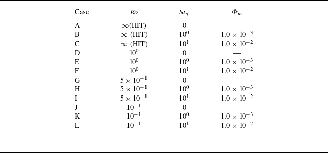
 Ro
 Stη
 Reλ≈90
 Φv=3.5×10⁻⁸

 G
 e1
 e2
 e3
 λ1
 λ2
 λ3
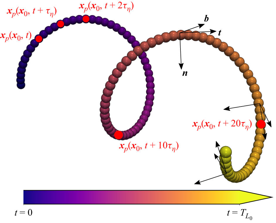
 {t,n,b}
 t=0
 t=TL0

 Ekin(t)/Ekin0

 Ro=100
 Ro=5×10⁻¹
 Ro=10−1
 E(k)
 E2-D(k)
 E3-D(k)
 Π(k)2-D-2-D
 Π(k)3-D-3-D
 Π(k)2-D-3-D

 t/TL0=65
 Ekin
 Ekinp(xp)=|vp(xp)|2/2
 Ro=100
 Ro=5×10⁻¹
 Ro=10−1
 Stη=0
 100
 101
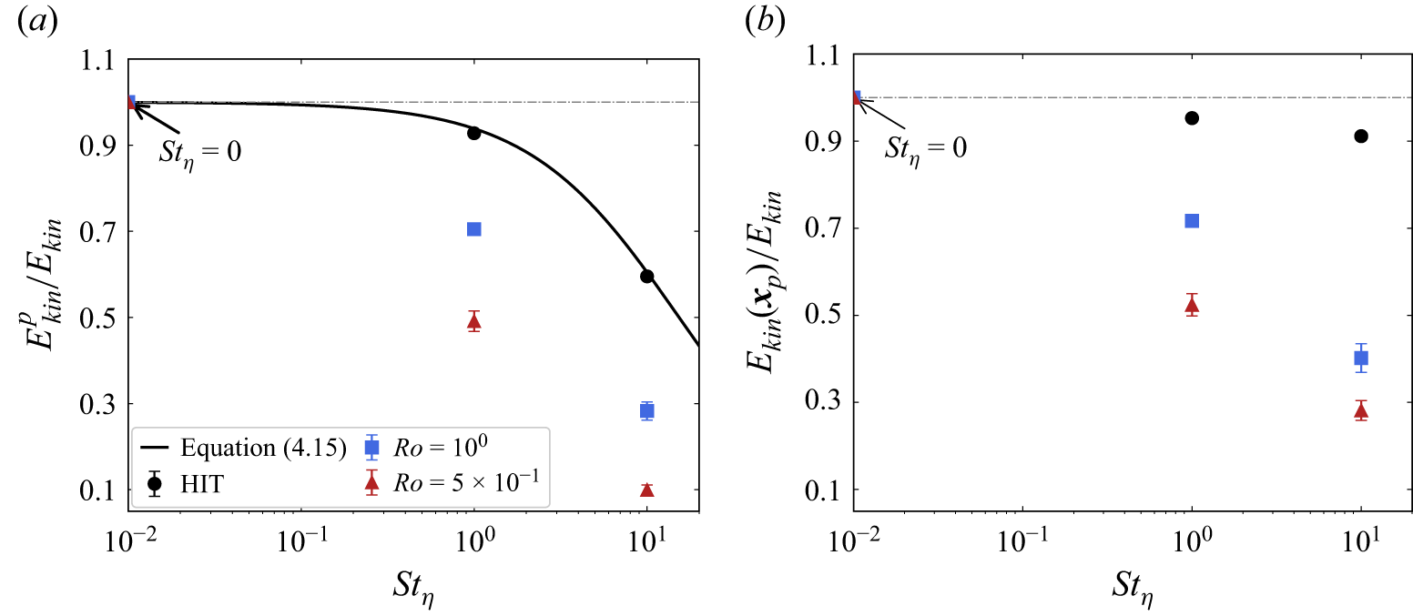
 Ekin

 Ro=100
 Ro=5×10⁻¹
 Ro=10−1
 Ekin,⊥=ux2+uy2
 x
 y
 2×η
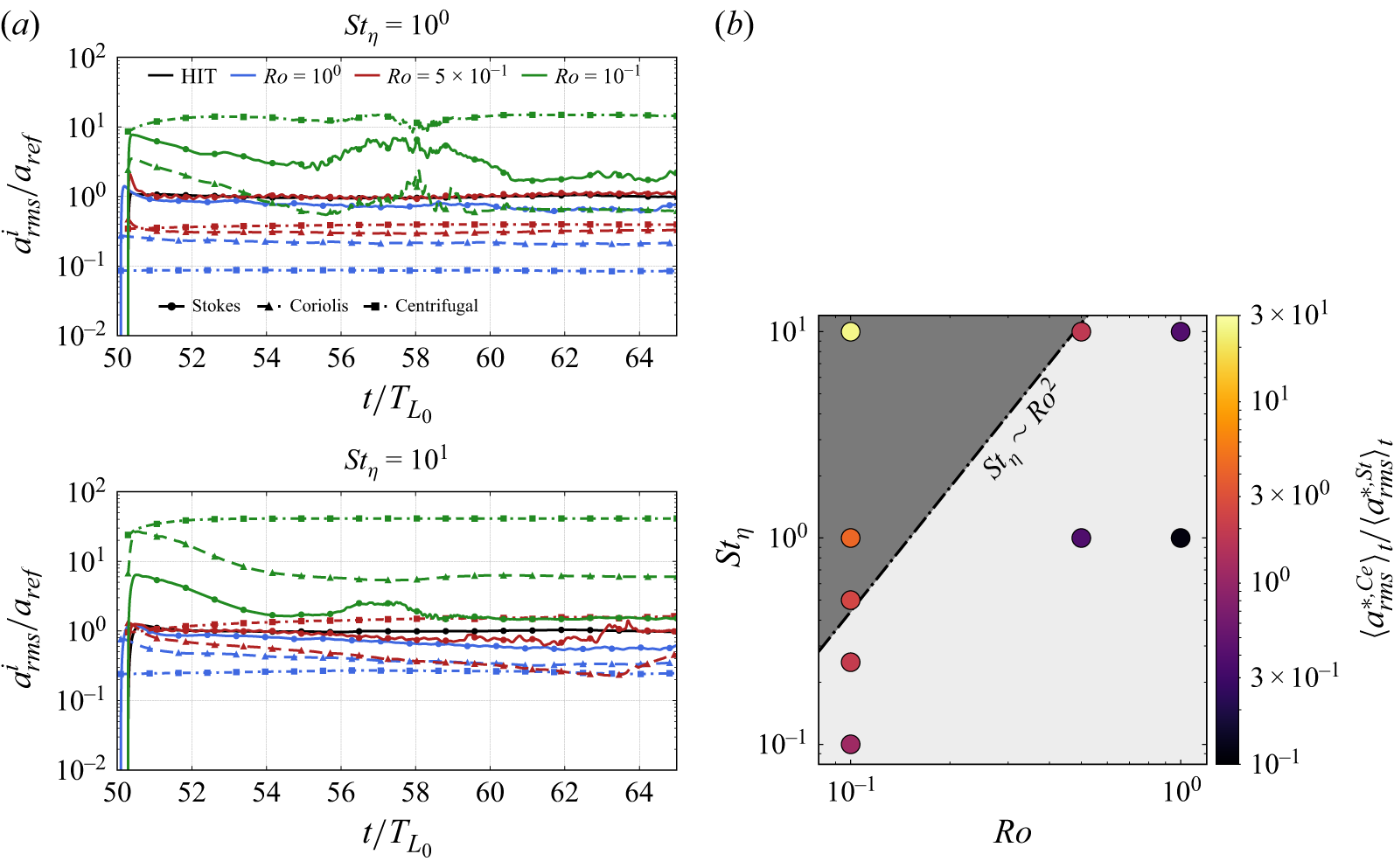
 aref
 Stη
 Stη
 Ro
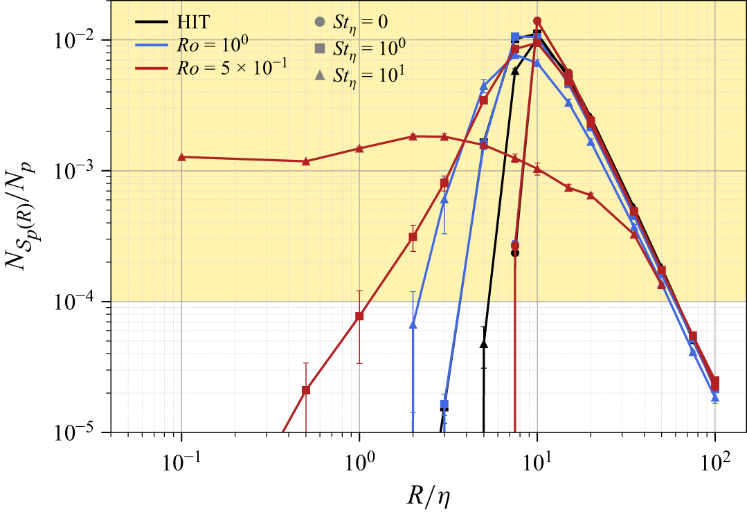
 NSp(R)
 Np
 R/η
 N⩾Nmin=20
 NSp(R)>102

 log10(Gαα/R2)
 R
 η
 Stη=0
 Stη=100
 Stη=101
 Ro=100
 Ro=5×10⁻¹

 Ro=100
 Ro=5×10−1
 x1c
 x2c
 x3c

 θ1
 θ2
 θ3
 Piso(θ)=sinθ
 Stη=0
 Stη=100
 Stη=101
 Ro=100
 Ro=5×10⁻¹

 50
 Stη=0
 Stη=100
 Stη=101
 Ro=100
 Ro=5×10⁻¹
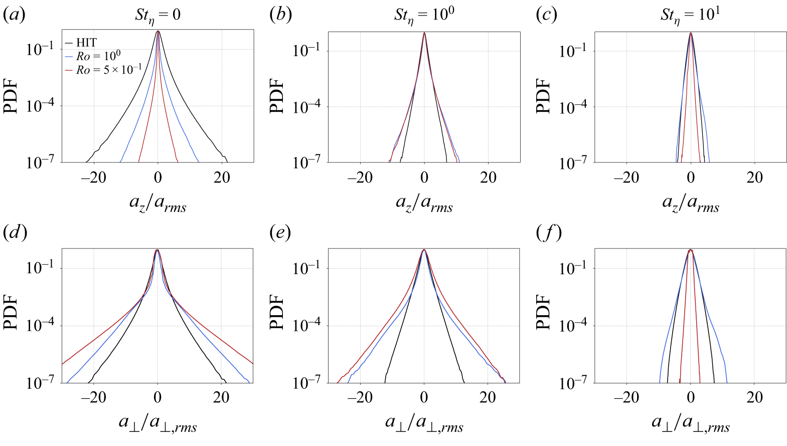
 az
 a⊥=(ax+ay)/2
 arms

 Stη
 Ro=100
 Ro=5×10⁻¹
 az
 a⊥
 Sa
 Fa
 arms/a0

 K
 T
 Stη=0,100,101
 Ro=100
 Ro=5×10⁻¹
 η
 Δt/τη=1,5,25
 (Kη)1
 (Kη)−5/2
 (Tη)0
 (Tη)−3
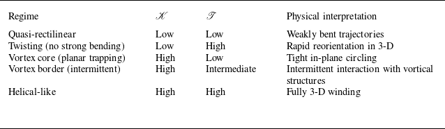

 PDF(Kη,a⊥/a⊥,rms)
 η
 Stη=0
 100
 101
 Ro=100
 Ro=5×10⁻¹

 Ro=100
 Ro=5×10⁻¹
 QA/⟨QΩ⟩
 RA/⟨QΩ⟩3/2
 QS/⟨QΩ⟩
 RS/⟨QΩ⟩3/2
 −QS/⟨QΩ⟩
 QΩ/⟨QΩ⟩
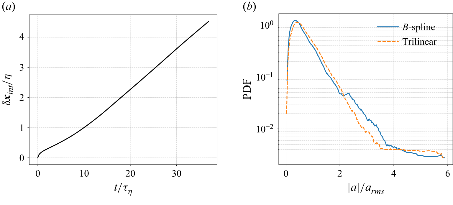
 B

 R/η
 NR⩾10
 NR⩾50
 ⟨NR∣NR⩾Nth⟩
 σ(NR)/⟨NR⟩

 Φm
 Stη=100
 Stη=101

 Open access

