


Introduction
The discovery of Heinrich events in the North Atlantic (i.e. episodes during which the ice streams that discharge ice sheets became enormously active, producing large numbers of icebergs possibly associated with a partial collapse of the ice sheets) provided new motivation for Antarctic research, especially for studies of the West Antarctic ice sheet, since its activity is also dominated by fast-flowing ice streams. In this regard, the following key questions may be formulated: (1) what is the modern configuration and behavior of the West Antarctic ice sheet (e.g. where is it changing and by how much?), (2) what is the climatic history of West Antarctica (e.g. was there an ice sheet present during the last interglacial?), (3) what are the leads and lags of West Antarctic ice-sheet advance and retreat with global sea levels and with glacial fluctuations in the Northern Hemisphere and other parts of the Southern Hemisphere?
Though the potential instability of the West Antarctic ice sheet was a central issue of numerous earlier studies (e.g. Reference HughesHughes, 1973; Reference MercerMercer, 1978; Reference Alley and WhillansAlley and Whillans, 1991), it is only recently that more comprehensive three-dimensional (3-D) models of the Antarctic ice sheet have been developed (Reference HuybrechtsHuybrechts, 1992; Reference Budd, Jenssen, Mavrakis and CouttsBudd and others, 1991). These models, however, consider large-scale ice-sheet dynamics as separate from mesoscale ice-stream dynamics (e.g. Reference MacAyealMacAyeal, 1992). This is because the thermal features of coastal ice streams, which attain just a few hundred kilometers in length, cannot be resolved in a large-scale model. It is not unlikely that the artificial horizontal diffusion inherent in numerical solutions of 3-D equations forces modelers to sacrifice mesoscale effects in favor of numerical stability.
Nevertheless, one should recognize that to answer the above questions, we must simulate the ice sheets with a 3-D model from which we can calculate the ice topography, the velocity of the ice flow, and the temperature distribution, to a level of accuracy necessary to produce ice streams internally without prescribing them. In the next section, we formulate an ice-sheet model utilizing a simple formula for the basal temperature that is free from an artificial horizontal diffusivity, and allows simulation of temperature structures that could be associated with ice streams. We shall demonstrate that applying our model to the late Pleistocene, ice-stream-like structures appear and disappear, and switch to active or stagnant modes, as a part of a single solution responding to external forcing.
The Model
Ice dynamics
The dynamic part of the model is governed by an equation representing a mass balance of the non-linear ice flow,
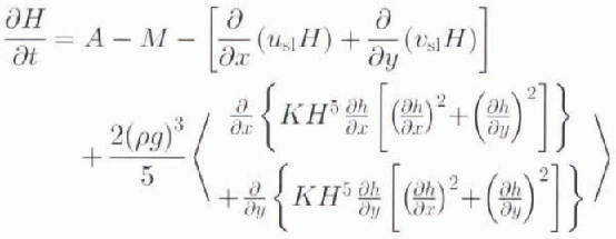
where H is the iee thickness; h is elevation, h = h′ + H ™ ξ; hʹ is the bedrock topography measured above sea level; hʹ = hʹ 0 − ζ, hʹ 0 is the “undisturbed” bedrock topography; ζ is the bedrock depression under the ice load; ξ is the change in the sea level; A is the accumulation rate of snow onto the ice sheet; M is the mean annual ablation; g and ρ are the gravity acceleration and the density of ice, respectively; n = 3, where n is a power degree and K is the vertically integrated temperature-dependent coefficient in Glen’s rheological law; and u sl and v sl are components of the sliding velocity. We restrict ourselves to studying grounded ice dynamics only, and leave aside the role of ice shelves. Thereby we accept the arguments of Reference Hindmarsh and PeltierHindmarsh (1993b) that, to the order of the commonly used approximations, ice-sheet mechanics do not require knowledge of the stress distribution across the transition sheet–shelf zone. However, we recognize that the mass balance of an ice sheet might be influenced strongly by thermal effects along the calving periphery of an ice sheet.
As the boundary condition for the model, we set H = 0 beyond the ground line, where the flotation condition,

is satisfied. Here, ρw is the density of the sea water. This
equation implies that the grounding line can advance due to bedrock rebound
and sea-level drop, and can retreat due to decreased ice thickness, bedrock
depression, and sea-level rise. It is noteworthy that the movement of the
grounding line is computed simply from the ice-sheet mass balance (Reference Hindmarsh and PeltierHindmarsh, 1993b). The above boundary
condition is equivalent to the assumption that the grounding line resides
somewhere between the last grounded point
 and the boundary point (H = 0) where the
ice-sheet profile, as determined by the numerical discretization, takes the
value
 . We allow Impossible ice-shelf grounding by calculating
the critical thickness of an ice shelf as
 (Reference Oerlemans and van der VeenOerlemans and van der
Veen, 1984), and consider an ice shelf to become grounded if

The bedrock is assumed to be depressed locally by the ice load (Reference Debonde and PeltierDeblonde and Peltier, 1993):
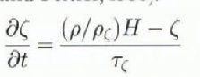
where τ ζ is the relaxation time constant and ρ ζ is the density of the bedrock.
A simple formula for the ice-sheet basal temperature
It has been noted (Reference HindmarshHindmarsh, 1993a; Reference Verbitsky and SaltzmanVerbitsky and Saltzman, 1995) that any errors in ice-topography calculations are non-lincarly amplified in the advective terms of the equation of heat transfer. Since the horizontal velocity of ice advection is proportional to the ice thickness to the power 2n + 1 (e.g. Reference VerbitskyVerbitsky, 1992), a 10% error in ice thickness for the conventional value of n = 3 leads to nearly a 100% error in horizontal velocity, which makes the accuracy of the temperature calculations rather dubious. Moreover, as we noted above, some mesoscale temperature features could be lost due to the artificial horizontal diffusion inherent in numerical solutions of the 3-D thcrmodynamical equation (e.g., Reference HuybrechtsHuybrechts, 1992). For all these reasons, one might be reluctant to expend significant effort in solving the full 3-D energy equation for an ice sheet, especially when a vertically integrated model is employed and the details of the vertical temperature structure are not a matter of concern. Here we suggest a simple formula for the basal temperature of an ice sheet, which is free from artificial diffusion effects, and at the same time is good enough to reproduce the large-scale features of a solution obtained from the 3-D energy equation.
It was shown by Reference Grigoryan, Krass and ShumskiyGrigoryan and others
(1976) and Reference MorlandMorland (1984)
that in the usual glaciological system the ratio of the conductive component
to the advective component of the heat flux above the bottom boundary layer
(BBL) is small, and an ice-flow trajectory has a near-constant temperature
determined by its value on the top surface of the ice sheet. We determine
the thickness of the BBL, η, from the balance of the
vertical diffusion, kT
zz, and advection of heat measured by uT
x (T is the temperature, u is
the horizontal velocity, and k is the thermal diffusivity
of ice). Scaling u from the mass-balance requirement
u = aL/H (H is the ice
thickness, a is the snowfall rate, and L
is the horizontal span), and setting
 and
 (thus assuming that vertical and horizontal temperature
gradients are of the same order of magnitude), we have (sec also Reference MorlandMorland, 1984):
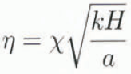
where X is a proportionality constant. Within the BBL, the vertical-heat diffusion is in balance with heating due to internal friction, f,

where λ is the thermal conductivity of ice.
At the bottom (z = 0)

where T
M is the pressure-melting temperature, and Q is
the geothermal heat flux that can be enhanced by the heat of basal sliding
 and by the heat of fusion Q″ if
T = T
M, where V
sl is the basal sliding velocity and
 is basal-shear stress. For the sliding velocity we adopt
the approximation of Grevc and Reference MacAyealMacAyeal
(1996):
 where k
sl is a constant. At z = η,

In accordance with the above, the temperature T b is assumed to be advected from the top surface of the ice sheet with the time lag H/a, and can be determined from the equation,

where T h is the temperature on the ice-sheet surface.
Solving Equation (5) with the boundary conditions of (6) and (7), we finally obtain the formula for the basal temperature T B,

A few remarks regarding this formula are appropriate. First, we want to clarify how horizontal advection is taken into account. Horizontal advection does not affect the basal temperature directly, since there is little horizontal advection within the BBL. However, horizontal advection affects the thickness of the BBL. In other words, in an active ice sheet undergoing an increased snowfall rate, the surface temperature T h penetrates deeper. This effect is taken into account by formulas (4) and (9). It must be recognized, however, that calculating T b by using Equation (8) may lead to some error (e.g. it docs not account for the temperature inversion effect); the results shown in the next section suggest that this error is not significant, but further comprehensive tests are necessary.
It is important to note that T B as represented by Equation (9) is time dependent. In our case, two time-scales are particularly important: the time-scale of thermal advection, τ = H/a, and the time-scale of dynamical adjustment to accumulation rate changes, τ 1. It can be shown (e.g. Reference WhillansWhillans, 1981) that for fixed margins τ 1 = τ (2n + 2) ≪ τ. Both of these time-scales enter the calculations through the application of Equations (4) and (8) to evaluate η and T b, respectively. Equation (8) operates with a time-scale τ. This means that if T h, changes, this change will be transmitted downward with a time-delay τ. Equation (4) is a steady-state formula, and η changes instantly. This means that if a changes, the basal temperature in the model will respond immediately. In reality, however, the restructuring of an ice sheet (i.e. the shape, stress, velocities, and ηadjustment) takes place with a time-scale τ 1. Though in the simple formula we satisfy the relation τ 1 ≪ τ by assuming τ 1 = 0, the relation τ 1 = τ/(2n + 2) is not satisfied. Only further tests can clarify whether this may be important.
The integral form of the frictional healing term,
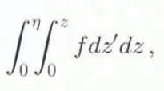
in Equation (9) does not mean that the internal friction is “spread” over the whole depth of the BBL instead of being concentrated near the bottom. In the model, frictional heating is calculated using the exact solution for the strain rate and shear stress. If at some point f is equal to zero the integral is not affected by that point.
The above formula for the basal temperature in Equation (9) will now supplement the dynamical part of the ice-sheet model (1). When the basal temperature reaches the pressure-melting point, a lubricating water layer forms and ice begins to slide at a rate proportional to the basal shear stress. In view of the uncertainties regarding the subglacial hydrology process (e.g. Reference HughesHughes, 1992), the coefficient k sl in the sliding law is in fact a free parameter; in our experiments ρgksl = 10 a−1. We assume the rheological coefficient K to be a function of basal temperature, and use the Reference ShumskiyShumskiy (1975) approximation, K = K 0 exp[−k(T M/T B − 1)], K 0 = 1.5 × 10⁻¹⁶ (Pa3 a)−1, k = 21.1. In all experiments, χ = 1, τ ζ = 3000 a, Q = 0.0546 W m−2.
Modeling the “Present-Day” Equilibrium Regime of the Antarctic Ice Sheet
We solved the model equations on a high-resolution (40 × 40 km) grid for values of the climatic temperature, bedrock topography, and snowfall rate adopted from (Reference HuybrechtsHuybrechts 1992, Reference Huybrechts1994). The equilibrium solution, which we associate with the “present-day” state (probably non-equilibrium), is shown in Figures 1 and 2 for some of the two-dimensional variables. It can be seen in Figure la that the ice-sheet model reproduces reasonably well the ice topography and velocity distribution of the present-day Antarctic ice sheet. We note first that the results resemble major features of the observed ice thickness. Deviations from observations (generally within 10–15% of the present-day thickness) may be attributed, indeed, to the model’s shortcomings, but might simply be a manifestation of the fact that the Antarctic ice sheet is not in a steady state, or that there are errors in the bedrock elevation data.
“Present-day” equilibrium regime of the Antarctic ice sheet: (a) ice thickness (m): (b) mean horizontal velocity (ma1): (c) thickness of the bottom-boundary layer(m): (d) heat influx due to internal friction and basal sliding in units of the geother-
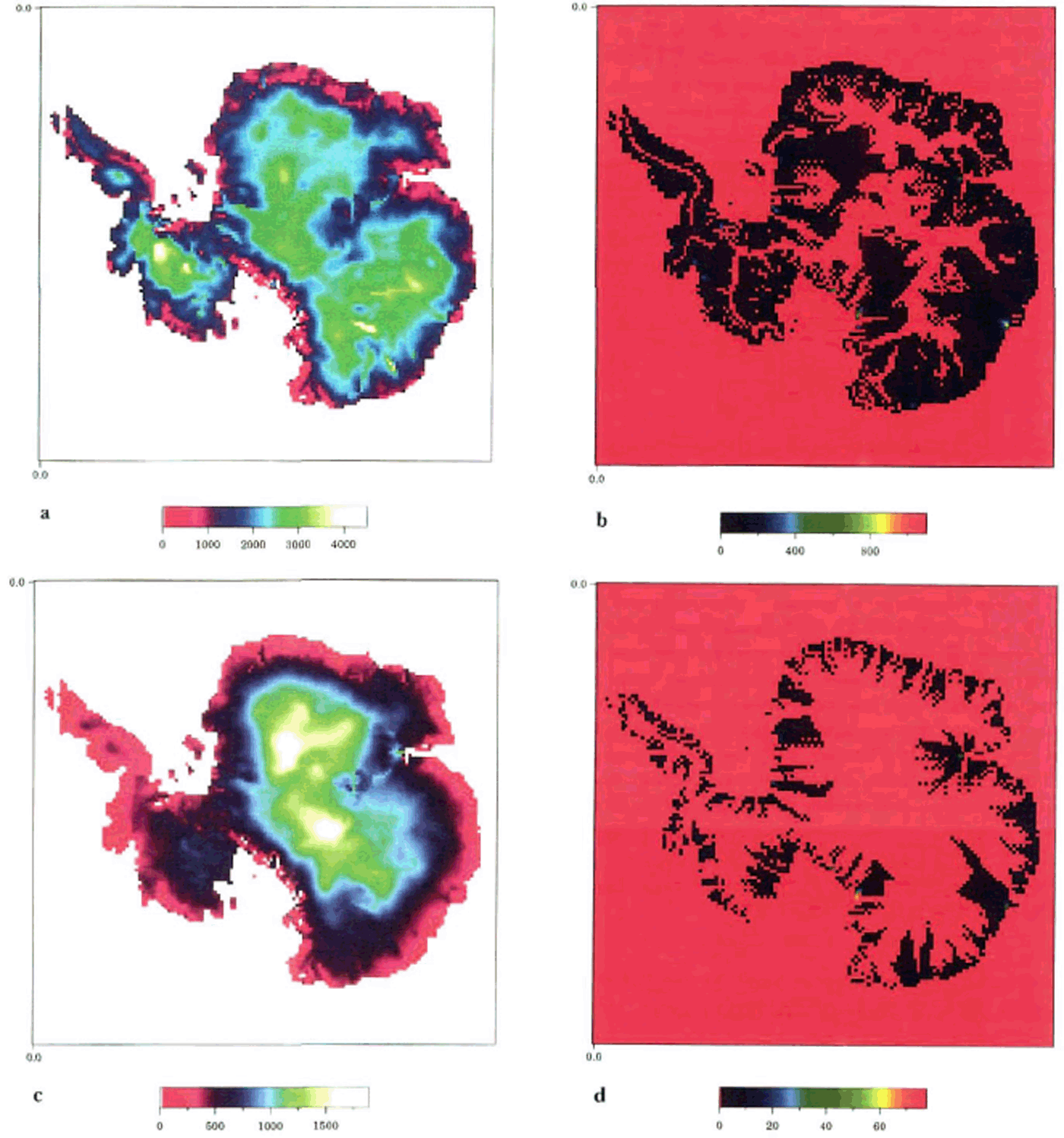
The vertically integrated velocity of ice flow (Fig. 1b) is small (a few meters per year) in the central part of an ice sheet and at ice divides, and reaches a few hundred meters per year near the grounding line. Points with maximum ice velocity identify all major ice streams and outlet glaciers. The thickness of the BBL, determined according to Equation (4), is shown in Figure 1c. Its value reaches roughly 1000 m in the central part of the ice sheet, and only a few hundred meters at the peripheral regions.
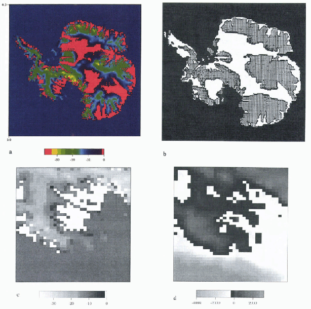
In Figure 1d we show the intensity of heating due to internal friction and basal sliding in units of the geothermal heat flux. One can see that geothermal heat flux dominates in central regions, but internal friction is much more significant near the ice-sheet edge. Figures 2a shows the calculated basal temperature, which also compares well with the shape and extent of the areas of melting and freezing temperature obtained by Reference HuybrechtsHuybrechts (1992) as a solution of the full 3-D thermodynamic equation (Fig. 2b). This implies that our simplified formula can represent the relevant thermodynamics. Moreover, our approach seems to allow us to simulate the fine temperature structure in the coastal zone.
At the West Antarctic Siple Coast, the bottom temperature has an interesting form: areas at the pressure-melting point are separated by strips of frozen-to-bed ice (Fig. 2c and d). Ifwe associate these features with ice streams, they are reminiscent of (1) Ice Streams A and B, uniting to form a single flow downstream, (2) a similar structure formed by Ice Streams D and E, and (3) the narrow Ice Stream C in the central part of the coast. Not only is the shape of these structures similar to the ice streams found on the Siple Coast, but their behavior is also similar in that their horizontal flow is dominated by the basal sliding, and is much faster than the flow of the neighboring ice. Although we recognize that these model-generated features are not ice streams in the fullest sense, since their horizontal velocities are still less than the observationally suggested values, in the following discussion we will refer to this pattern as a “stream-like structure” or “ice streams”.
Increased snowfall rates intensify the advection of the cold temperature from the top of the ice sheet to its bottom, and a consequent decrease in the bottom temperature might be expected due to thinning of the BBL. To explore this possibility, we performed a sensitivity experiment, increasing the snowfall rate over the Siple Coast. In Ice Streams A and B, D and E, an increase in the frictional heating offset the advection effect, but friction in Ice Stream C was not strong enough to counteract it and Ice Stream C switched from an active sliding mode to slow creeping mode. The detailed analysis undertaken in the next section will explain the reason for this.
Modeling the Antarctic Ice Sheet During the Last Ice Age
A block-scheme of the experimental set-up is shown in Figures 3. The model variables are shown in rectangles, external forcing (empirical data) is shown in circles, arrows indicate interconnection between variables, and plus and minus signs indicate positive and negative feedbacks, respectively. Wc forced our Antarctic ice-sheet model with sea-level and temperature changes, invoking two widely accepted, independent measures of temperature and ice volume (rescaled in terms of the sea level, z): the Vostok core-temperature measurements (Reference JouzelJouzel and others, 1993) and the SPECMAP δ 18O estimate (Reference Imbrie, Imbrie, Hays, Kukla and SaltzmanImbrie and others, 1984). Although questions arise concerning the absolute chronologies of these two measures, it is of interest to examine their implications, taking them at face value as the best estimates currently available. Some support for these estimates has come from recent studies with regard to temperature changes (Shackleton and others, 1992) and ice volume (Sowers and others, 1993).
For surface temperature, we adopted Huybrechts (1994) formula:

where ϕ is latitude, α, β, γ are coefficients, and ΔT v is the temperature change as represented by the Vostok measurements. To calculate mean annual ablation, we used the empirical formula of Khodakov (1965), based on measurements from glaciers and ice caps:

This formula gives results similar to Pollard's (1980) parameterization. Here T S is the summer temperature determined according to Huybrechts (1994) as

We represent the snow accumulation rate as the sum of its present-day value. A 0 Huybrechts. (1992) and a forced departure, δA. If we assume that A is temperature dependent (Huybrechts, 1994), i.c.

in the range of temperatures presently prevailing on Antarctica, we have

For the temperature departure. ΔT, we employ the measurements of the temperature at the Southern Ocean core
MD88-770 (46°S, 96° E) studied by Reference SowersSowers and others (1993) assuming that these variations might be a better proxy for moisture availability over the Antarctic continent than the Vostok temperatures. In Figures 4 we show the assigned forcing (i.e. sea level, Vostok, and Southern Ocean temperature changes). The coevolution of these three variables forms a complicated trajectory in phase space (Reference Saltzman and VerbitskySaltzman and Verbitsky, 1994).
“Presently” equilibrium regime of the Antarctic ice sheet: (a) the calculated basal temperature. Red represents the pressure melting point; (b) the same from Reference HuybrechtsHuybrechts (1992). White represents the pressure melting point; (c)–(d) the calculated basal temperature (white is at the pressure melting point) and the bedrock topography for the Siple Coast region
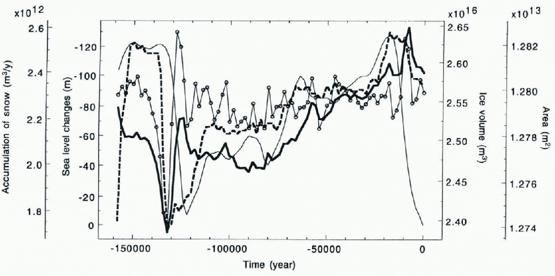
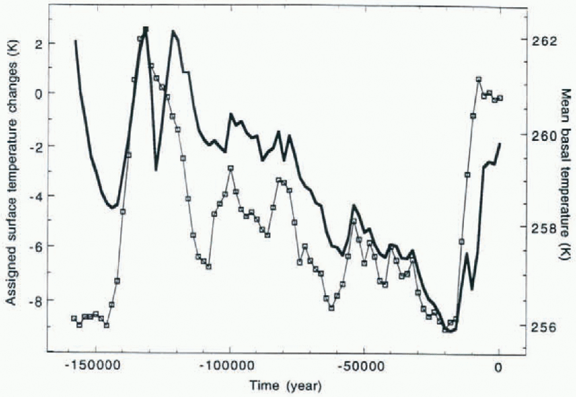
In Figures 5 we show the calculated changes in the Antarctic ice-sheet volume and area along with the assigned sea-level changes and mass balance generated according to Equations (10) – (14). One may note that ice-sheet area is influenced mainly by changes in sea level. On the other hand, ice-sheet volume reproduces the tendency of the prescribed sea-level changes on the long time-scale (~100ka), increasing while the sea level drops and decreasing when sea level rises, but on a shorter time-scale (~10ka) ice volume is highly sensitive to the mass balance. As a result, Antarctic ice volume reached its maximum not during the last glacial maximum in the Northern Hemisphere, 20 ka ago, but later during the interglacial when a large positive mass balance is assumed to have existed due to relatively high ocean temperature. Figures 6 shows the assigned surface temperature changes, and the calculated mean basal temperature that appears to follow the surface temperature with a time lag. Irregularities at 128 ka and 10 ka reflect advective cooling due to increased snowfall rates.
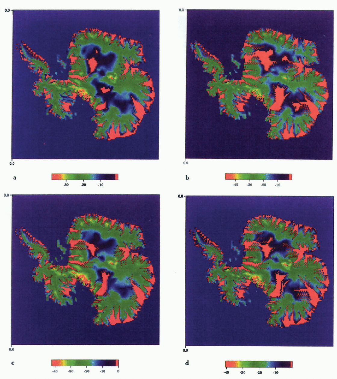
In Figures 7 we plot the calculated basal temperature at 128 ka, 50 ka, 10 ka, and 0 ka (end of the experiment). Consistent with Figures 6. the basal temperature generally decreases with time as the assigned decrease in the surface temperature is advected toward the bottom. According to the model, the present-day temperature still “remembers” the cold conditions of the last glacial maximum.
The stream-like structure of the West Antarctic Siple Coast found in the steady-state solution appears to be very robust, and can be observed during the whole glacial cycle under a wide range of external forcing. Interestingly, as in the sensitivity experiment described earlier, Ice Stream C again shows its “readiness” to stagnate and switches to a slow mode during the penultimate interglacial at 128 ka and partially at 10 ka during the last interglacial when snowfall rates were high. The question arises as to why Ice Stream C is more vulnerable to increased snowfall rates.
Block scheme of the numerical experiment. See details in the text

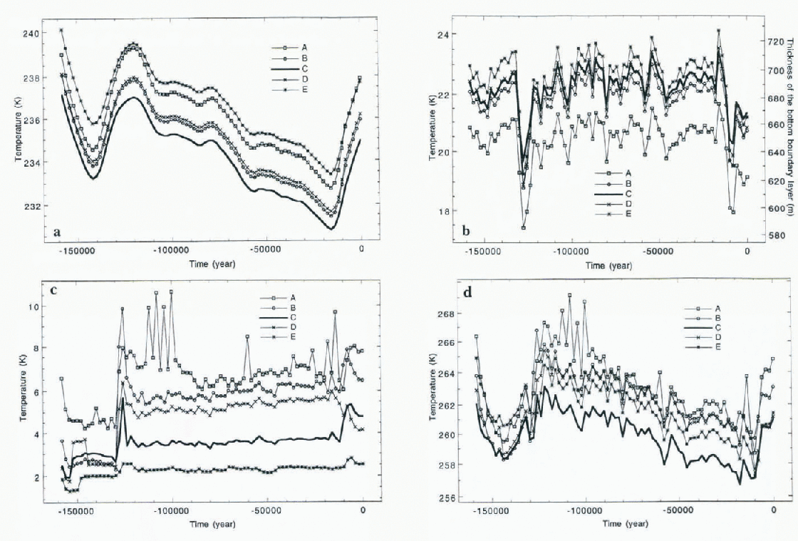
To answer this question, we have compared the terms of Equation (9) for selected points on Ice Streams A–E. The results are shown in Figures 8. We note first (Fig. 8a), that, in the model, Ice Stream C has the lowest “background” temperature T b, (i.e. the temperature advected from the top of the ice sheet). Figures 8b shows evolution of the BBL thickness and, being multiplied by Q/λ, shows the combined contribution of the geothermal heat flux and thermal advection to the basal temperature. It is noteworthy that two major basal cooling events are observed during the last and penultimate interglacials when snowfall rates are high.
External forcing: surface-temperature changes (solid line) from Vostok core measurements (Reference JouzelJouzel and others, 1993); the SPECMAP δ18O estimates (Reference Imbrie, Imbrie, Hays, Kukla and SaltzmanImbrie and others, 1984) in terms of the sea-level changes (dotted line), and measurements of the temperature changes at the Southern Ocean core MD88-770 (Reference SowersSowers and others, 1993), dashed line.

In Figures 8c we show the contribution of the internal heat flux to the basal temperature,
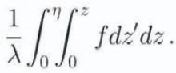
The penultimate and the last interglaeials are also visible in Figures 8c: periods of high snowfall rales are marked by increased internal friction. It is of critical importance that the internal friction in Ice Stream C is low. We show the sum,
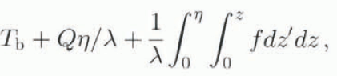
in Figures 8d. The combination of coldest surface temperature and low intensity of internal friction gives Ice Stream C the lowest possibility to counteract the advective cooling. At 128 ka, when snow accumulation was at its maximum, advective cooling caused the freezing of Ice Stream C’s base. At the present day (Fig. 7d), most of the bed of Ice Stream C is thawed with two frozen sticky spots, which is consistent with findings of Reference Anandakrishnan and AlleyAnadakrishnan and Alley (1994).
Modeling the Antarctic ice sheet during the last ice age. Calculated changes in Antarctic ice sheet volume (thick solid line) and area (dashed line), along with assigned sea-level changes (thin solid line) and surface mass balance (circled line)
Modeling the Antarctic ice sheet during the last ice age. Calculated mean basal temperature (thick solid line) along with assigned surface-temperature changes (squared line)
Calculated basal temperature at (a)128 ka, (b)50 ka, (c) 10 ka, and (d) 0 ka. Red represents the pressure-melting point
Contribution of different factors to basal temperature of Ice Streams
A–E: (a) advected surface temperature. Tb; (b) thickness of
the bottom-boundary layer, η. and contribution of the geothermal flux,
Qη/λ (c) coulribution of the internal heat flux
 (d) the sum of the above,

Thus, our investigation indicates that the reduced internal frietion of Ice Stream C and a low surface temperature are possibly responsible for its stagnation. The implications of Equation (10) are straightforward concerning T h and do not require further discussion. In order to determine why internal friction in Ice Stream C is low, additional experiments were performed.
In the first experiment, we replaced the real bedrock topography of the Siple Coast, shown in Figures 2d, by a flat plane. As a result, the basal temperature field at Siple Coast displays only one strip of frozen ice. Topographically, this strip is under the divide that is located close to the present-day position of Ice Stream C. In turn, this divide appears to be due to the specific shape of the coastline that has a clearly identified cape in the southern part of the Siple Coast (Fig. 2d). This ridge, and the strip of cold temperature, disappear when we change the shape of the coastline by replacing the cape by a straight coastline. We may surmise, therefore, that peculiarities of local topography (including the shape of the coastline) may create a situation in which an ice stream develops at a divide, and consequently has a lower surface temperature, and reduced shear stresses and internal friction. It is not unlikely that this situation may be characteristic of Ice Stream C.
Conclusions
We used a 3-D (although vertically integrated). high-resolution (40 × 40 km), non-linearly v iscous, non-isothermal ice-sheet model to calculate the “present-day” equilibrium regime of the Antarctic ice sheet and its evolution during the last glacial cycle. Since the model is vertically averaged, the only temperature field we needed was the basal temperature, which determines regions of frozen and melting ice at the bottom of an ice sheet, and consequently determines the sliding component of the ice flow. In the course of our study, we suggested an approximate formula for ice-sheet basal temperature, based on scaling the thermodynamic equation for the ice flow. To test this formula, we simulated the equilibrium regime of the Antarctic ice sheet under the present-day climatic conditions. A steady-state solution for the shape and extent of the areas of basal melting or freezing temperature turned out to be in good agreement with those obtained from the solution of full 3-D thermodynamic equation. As an unexpected main result of this experiment we found that the solution for the basal temperature field of the West Antarctic Siple Coasi reproduced areas at the pressure-melting point separated by strips of frozen-to-bed ice, the structure of which is suggestive of Ice Streams A–E. At this point it is difficult to speculate why this result was not obtained previously in other large-scale models of the Antarctic ice sheet. We can only guess that mesoseale temperature features could be lost due to the artificial horizontal diffusion inherent in numerical solutions of the 3-D thermodynamic equation. A comprehensive experimental run and intercomparison with other models is needed to verify our supposition.
This simulated stream-like structure appeared to be robust, preserving its features under the wide range of climatic changes din ing the last glacial cycle (though Ice Stream C seemed to be more vulnerable to the stagnation, switching to a passive mode during the penultimate interglacial). We speculated that peculiarities of the local topography determined the unique behavior of Ice Stream C: reduced basal stress and, consequently, relatively weak warming due to internal friction and basal sliding, was unable to counteract advective cooling during the periods of increased snowfall rates.
This conclusion should be regarded as tentative, however, for the following reasons: the dynamics of the subglacial processes (e.g. the dynamics of the deformable till, anad the generation and drainage of melting water) are accounted for by the simplest form of a sliding law (Reference Greve and MacAyealGreve and MacAyeal, 1996) that does not depend on either the intensity of basal melting or on the hydraulic properties of the sediments. We also excluded the whole class of physical phenomena characteristic of the transition zone between an ice sheet and ice shell, which might be important in describing the grounding-line dynamics (e.g. Reference Alley and WhillansAlley and Whillans, 1984; Reference Van der Veen, Van der Veen and OerlemansVan der Veen, 1987; Reference HughesHughes, 1992). It is likely, also, that our resolution is not sufficiendy high to allow final conclusions to be drawn. We also should not forget that the way we assigned external forcing, though based on the most reliable data available is no mure than a reasonable speculation about the possible changes of climatic conditions during the last glacial cycle.
For the future we plan to use an atmospheric general circulation model coupled with the mesoscale atmospheric model nested in the southern polar region to improve the representation of snowfall rates and surface temperature. Until this is completed, we probably have to regard our attempt to model the Antarctic ice sheet during the last ice age as a comprehensive sensitivity experiment rather than a simulation of real evolution. Consequently, our study is not intended to replace existing theories of ice streams, or to challenge the hypothesis about Ice Stream C stagnation (e.g. Reference Alley, Anandakrishnan, Bentley and LordAlley and others, 1994; Reference Fowler and JohnsonFowler and Johnson, 1995). What we do want to say is that, according to the model, some distinctive features of ice-stream structure found at the Siple Coast may have deep roots in a large-scale topography that is able to pre-determine the development of some of the properties we have observed.
Epilogue
Hindmarsh has criticized the model on the grounds that it is a parameterization of two thermal-transport processes (advection and diffusion) that are treated explicitly in most models and regarded as being well understood by most glaciologists. Hindmarsh Turtherstatesthat since the model is a parameterization, the results are difficult to interpret — for example, do they work well because they over- or underestimate the contributory processes of conduction and advection? Moreover, since they are parameterizations, their range of validity is not clearly understood.
We nevertheless note, that a model cannot be wrong merely because it is simple. We need a simple model when more sophisticated models are not helpful (for whatever reasons) or when they are difficult to understand. In our case, 3-D models are not yet able to resolve ice streams.
Therefore, we used a simple model (which contains all of the qualitative physics contained in the 3-D model) to generate some ideas concerning Antarctic ice stream behavior and Ice Stream C stagnation in particular. We now challenge those who have a more sophisticated (but at the same time more realistic) model to test these ideas.
Acknowledgements
This work has been supported by the Office of Polar Programs (Polar Glaciology Program) of the National Science Foundation under grant OPP-9319674, and by NASA (Polar Research Program) under grant NAGW-4197, both at Yale University. We are grateful to P. Huybrechts for his generous help with the field data, and R. Hindmarsh and K. Cuffey for their friendly and constructive reviews.



