





1. Introduction
Recent optimisation (Landreman & Paul Reference Landreman and Paul2022; Goodman et al. Reference Goodman, Mata, Henneberg, Jorge, Landreman, Plunk, Smith, Mackenbach, Beidler and Helander2023) of stellarator equilibria has reduced orbit losses of fusion-born energetic ions to levels compatible with fusion power plant (FPP) design. This has motivated academic and private research (Gates et al. Reference Gates2025; Goodman et al. Reference Goodman2025; Hegna et al. Reference Hegna2025; Lion et al. Reference Lion2025) to develop a physics basis for stellarator FPPs. In addition to sufficiently low equilibrium losses, a viable FPP design needs to mitigate prompt energetic ion losses induced by shear-Alfvén wave (SAW) perturbations, which are known to produce significant transport in tokamaks (see Breizman & Sharapov Reference Breizman and Sharapov1995; Sharapov Reference Sharapov2021 and references therein). Various kinds of Alfvénic waves are observed in both tokamaks and stellarators, excited by inverse Landau damping interaction with energetic particles (Rosenbluth & Rutherford Reference Rosenbluth and Rutherford1975), by ion temperature gradients (Zonca et al. Reference Zonca, Chen, Dong and Santoro1999), by electron pressure gradients (Heidbrink et al. Reference Heidbrink2021) or through nonlinear coupling to ion temperature gradient (ITG) turbulence (Riemann et al. Reference Riemann2025). Accordingly, there is significant recent interest (White et al. Reference White, Bierwage and Ethier2022; Paul, Mynick & Bhattacharjee Reference Paul, Mynick and Bhattacharjee2023) in assessing energetic particle losses from stellarators in the presence of SAWs. These initial studies demonstrated that resonant SAW perturbations can drive significant losses of fusion-born alphas in FPP designs at normalised perturbation amplitudes that are consistent with previous experiments (see Toi et al. Reference Toi, Ogawa, Isobe, Osakabe, Spong and Todo2011; Nishimura et al. Reference Nishimura, Todo, Spong, Suzuki and Nakajima2013 and references therein). Stellarator FPP designs, therefore, require an assessment of SAW stability in the presence of energetic fusion products (Varela et al. Reference Varela, Spong, Garcia, Ghai and Ortiz2024), and wave-induced transport analysis (Hegna et al. Reference Hegna2025) as part of their physics baseline. Besides FPPs, sufficient confinement of energetic particles is necessary for a viable design of a beam-driven stellarator neutron source like the recently proposed EOS device (Swanson et al. Reference Swanson, Gates, Kumar, Martin, Kruger, Dudt and Bonofiglo2025).
Previous SAW-induced transport studies (White et al. Reference White, Bierwage and Ethier2022; Paul et al. Reference Paul, Mynick and Bhattacharjee2023) considered optimised stellarator equilibria and identified stochastic ion transport as a significant loss channel. Resonance overlap analysis for precisely quasi-axisymmetric (QA) and quasi-helical (QH) equilibria (Paul et al. Reference Paul, Mynick and Bhattacharjee2023) established that increased helicity of constant magnetic field-strength
 $B_0$
lines in the QH case suppresses stochastic ion transport relative to QA stellarators. This study also demonstrated that, in stellarator FPPs, SAW perturbations resonant with passing fusion-born alpha particles can drive significant prompt loss of these particles. However, the study used ad hoc shear-Alfvén perturbations, whereas self-consistent transport assessment requires perturbations compatible with equilibrium plasma parameters. The physics of Alfvénic perturbations in tokamaks and stellarators is subject to active research, and can require kinetic description (Chen & Zonca Reference Chen and Zonca2016). In this work, we use the minimal model for SAWs in stellarators, given by the ideal, incompressible Alfvén vorticity equation, implemented in the AE3D code (Spong, D’azevedo & Todo Reference Spong, D’azevedo and Todo2010). Although this minimal model does not address stability of SAW and neglects acoustic–Alfvén coupling and kinetic effects relevant (Weller et al. Reference Weller, Anton, Geiger, Hirsch, Jaenicke, Werner, Sallander and Spong2001; Kolesnichenko et al. Reference Kolesnichenko, Lutsenko, Thomsen, Yakovenko, Geiger and Werner2008) to low frequency modes, it provides Alfvén wave perturbations consistent with equilibrium magnetic field. Furthermore, given that much recent research is focused on quasi-isodynamic (QI) designs (Goodman et al. Reference Goodman, Xanthopoulos, Plunk, Smith, Nührenberg, Beidler, Henneberg, Roberg-Clark, Drevlak and Helander2024), which are closer to quasi-poloidal (QP) symmetry, it is instructive to extend the previous QA and QH resonance analysis (Paul et al. Reference Paul, Mynick and Bhattacharjee2023) to the general quasi-symmetric (QS) case. In this work, we extend previous resonance analysis to general QS equilibria and investigate prompt stochastic ion losses driven by self-consistent shear-Alfvén perturbations.
The rest of the paper is organised as follows. In § 2, we discuss the SAW perturbation model, the drift transport model and the diagnostic tools (Duignan & Meiss Reference Duignan and Meiss2023) for analysing particle stochasticity. In § 3, we extend the previous analysis to the case of general quasisymmetry, and apply the presented assessment framework to several optimised stellarator equilibria. In § 4, we summarise and conclude.
2. Model description
This section describes a drift kinetic, ideal reduced magnetohydrodynamic (MHD) model of ion transport in stellarators, in the presence of SAWs consistent with the equilibrium
 $B_0$
field and Alfvén velocity
 $v_{\mathrm{A}}$
profile. In this section and throughout the paper, we use SI units for dimensional quantities.
The guiding centre dynamics of a particle of mass
 $M_{\mathrm{s}}$
and charge
 $q_{\mathrm{s}}$
, moving in the equilibrium magnetic field
 $\boldsymbol{B}_0=\boldsymbol{\nabla }\times \boldsymbol{A}_0$
with vector potential
 $\boldsymbol{A}_0$
in the presence of a shear-Alfvén wave perturbation with magnetic field
 $\delta \boldsymbol{B}=\boldsymbol{\nabla }\times \alpha \boldsymbol{B}_0$
, is described by the Lagrangian (Littlejohn Reference Littlejohn1983)
 \begin{align} L\left(\boldsymbol{R},\frac {{\rm d}{\boldsymbol{R}}}{{\rm d}t},v_{\|},t\right)=q_{\mathrm{s}}\left(\boldsymbol{A}_0+\alpha \boldsymbol{B}_0+\frac {M_{\mathrm{s}}v_{\|}}{q_{\mathrm{s}}B_0}\boldsymbol{B}_0\right)\boldsymbol{\cdot }\frac {{\rm d}{\boldsymbol{R}}}{{\rm d}t}-\frac {M_{\mathrm{s}}v_{\|}^2}{2}-\mu B_0-q_{\mathrm{s}}\delta \varPhi , \end{align}
where
 $\boldsymbol{R}$
is the position of the particle,
 $t$
is time,
 $B_0$
is the equilibrium magnetic field strength,
 $v_{\|}=\boldsymbol{v}\boldsymbol{\cdot }\boldsymbol{B}_0/B_0$
is the component of the particle’s velocity
 $\boldsymbol{v}$
along
 $\boldsymbol{B}_0$
,
 $\mu =M_{\mathrm{s}}(v^2-v_{\|}^2)/(2{B}_0)$
is the magnetic moment and
 $\delta \varPhi$
is the scalar potential of the SAW. The electric field of the transverse SAW is normal to
 $\boldsymbol{B}_0$
, so the scalar
 $\delta \varPhi$
and vector
 $\alpha \boldsymbol{B}_0$
potentials are related by the condition
 \begin{align} \boldsymbol{B}_0\boldsymbol{\cdot }\left (\frac {\partial \alpha \boldsymbol{B}_0}{\partial t}+\boldsymbol{\nabla }\delta \varPhi \right )=0\Rightarrow \boldsymbol{\nabla} _{\|}\delta \varPhi =-B_0\frac {\partial \alpha }{\partial t}, \end{align}
where
 $B_0\boldsymbol{\nabla} _{\|}=\boldsymbol{B}_0\boldsymbol{\cdot }\boldsymbol{\nabla}$
is the derivative along the magnetic field. Because of (2.2), the transverse SAW is fully described by its scalar potential
 $\delta \varPhi$
. In the flute-reduced
 $k_\|/k_\perp \ll 1$
incompressible ideal MHD model (Kruger, Hegna & Callen Reference Kruger, Hegna and Callen1998),
 $\delta \varPhi$
satisfies the Alfvén vorticity equation
 \begin{align} \omega ^2 \boldsymbol{\nabla }\boldsymbol{\cdot }\left (\frac {1}{v_{\mathrm{A}}^2}\boldsymbol{\nabla }\delta \varPhi \right )+ B_0\boldsymbol{\nabla} _{\|}\left [\frac {1}{ B_0}{\nabla} ^2\left (\boldsymbol{\nabla} _{\|}\delta \varPhi \right )\right ]=0, \end{align}
where
 $k_\|$
and
 $k_\perp$
are wave vector components along and normal to the equilibrium field
 $\boldsymbol{B}_0$
,
 $\omega$
is the frequency of the SAW and
 $v_{\mathrm{A}}^2=B_0^2/(\mu _0 \rho _0)$
, where
 $\rho _0$
is the plasma mass density and
 $\mu _0$
is the vacuum permeability. The vorticity eigenvalue problem (2.3) with the conducting shell
 $\delta \varPhi =0$
boundary condition is the minimal model for SAWs; it represents charge conservation
 $\boldsymbol{\nabla }\boldsymbol{\cdot }\boldsymbol{j}=0$
in ideal MHD, where
 $\boldsymbol{j}$
is the plasma current, and neglects compression
 $\gamma =0$
effects from the finite specific heat ratio
 $\gamma$
.
Because the coupling between shear-Alfvén and acoustic waves scales with plasma pressure (Cheng & Chance Reference Cheng and Chance1985), neglect of compression effects in (2.3) is justified for the reduced MHD ordering model when the ratio of plasma pressure to the magnetic field pressure
 $\beta$
satisfies
 $\beta \lesssim k_\|/k_\perp$
. Larger
 $\beta$
values can (Turnbull et al. Reference Turnbull, Strait, Heidbrink, Chu, Duong, Greene, Lao, Taylor and Thompson1993) lead to a pressure-induced gap in the continuum and cause mixing of SAW and acoustic branches. Moreover, at sub-geodesic-acoustic-mode frequencies, finite diamagnetic frequencies and anisotropic pressure support drift-sound eigenmodes (Weller et al. Reference Weller, Anton, Geiger, Hirsch, Jaenicke, Werner, Sallander and Spong2001; Kolesnichenko et al. Reference Kolesnichenko, Lutsenko, Thomsen, Yakovenko, Geiger and Werner2008) absent in the ideal MHD model.
The Ampere’s law response in (2.3) is simplified by assuming that the wave vector’s components along
 $k_\|$
and normal
 $k_\perp$
to the equilibrium
 $\boldsymbol{B}_0$
field are flute ordered,
 $k_\|/k_\perp \ll 1$
. Furthermore, pressure and parallel equilibrium current
 $\boldsymbol{j}_0$
are neglected to exclude current and pressure driven instabilities (Hazeltine & Meiss Reference Hazeltine and Meiss2003). Retaining the pressure gradient was shown (Fu & Cheng Reference Fu and Cheng1990; Chu et al. Reference Chu, Greene, Lao, Turnbull and Chance1992) to shift SAW eigenfrequencies toward the lower gap boundary and modify the radial eigenstructure, although these corrections are small for the low-
 $\beta$
equilibria. These simplifications leave only unconditionally stable SAWs with frequency
 $\omega$
given by
 \begin{align} \omega ^2=\frac {\int \mathrm{d}^3\boldsymbol{r}|\boldsymbol{\nabla }\boldsymbol{\nabla} _\| \delta \varPhi |^2}{\int \mathrm{d}^3\boldsymbol{r}|\boldsymbol{\nabla }\delta \varPhi |^2/v_{\mathrm{A}}^2}\gt 0. \end{align}
It is convenient to solve the vorticity equation (2.3) in Boozer coordinates (Garren & Boozer Reference Garren and Boozer1991) for the equilibrium field
 $\boldsymbol{B}_0$
, because the derivative
 $\boldsymbol{\nabla} _\|$
along
 $\boldsymbol{B}_0$
has a particularly simple form in these coordinates. Therefore, ideal MHD (e.g. the AE3D code described in Spong et al. Reference Spong, D’azevedo and Todo2010) and gyrofluid (e.g. the FAR3D code described in Varela et al. (Reference Varela, Spong, Garcia, Ghai and Ortiz2024)) codes represent the wave potential as a superposition of Fourier harmonics in Boozer angles
 \begin{align} \delta \varPhi =\sum _{m,n}\varPhi _{m,n}(s)e^{i(m\theta -n\zeta +\omega t+\varphi _{m,n})}, \end{align}
where the sum is over harmonics with phase
 $\varphi _{m,n}$
, radial profile
 $\varPhi _{m,n}(s)$
and with poloidal
 $\theta$
and toroidal
 $\zeta$
Boozer angle mode numbers
 $m$
and
 $n$
, respectively. The radial profile of the harmonic amplitude
 $\varPhi _{m,n}(s)$
is a function of
 $s=\psi /\psi _{\mathrm{total}}$
, the toroidal flux
 $\psi$
normalised by its total value
 $\psi _{\mathrm{total}}$
. In Boozer coordinates, the contra- and covariant representations of the equilibrium
 $\boldsymbol{B}_0$
field are given by
 \begin{align} \boldsymbol{B}_0=\psi _0\boldsymbol{\nabla }s\times \boldsymbol{\nabla }\theta -\iota \psi _0\boldsymbol{\nabla }s\times \boldsymbol{\nabla }\zeta =K\boldsymbol{\nabla }s+I(s)\boldsymbol{\nabla }\theta +G(s)\boldsymbol{\nabla }\zeta , \end{align}
where the rotation transform
 $\iota =\mathrm{d}\psi _{\mathrm{p}}/\mathrm{d}\psi$
is the rate of change of poloidal
 $\psi _{\mathrm{p}}$
with respect to toroidal
 $\psi$
flux. In what follows, we neglect (White Reference White2017) the radial covariant
 $K=0$
component of the magnetic field, consistent (Imbert-Gérard et al. Reference Imbert-Gérard, Paul and Wright2024) with the low-
 $\beta$
assumption used for neglecting compressibility effects.
In stellarators, poloidal current
 $G$
is commonly (Helander Reference Helander2014) larger than the toroidal current
 $I$
. Furthermore,
 $I\ll G$
follows from the near axis expansion (Landreman & Sengupta Reference Landreman and Sengupta2018) in stellarators with large aspect ratio
 $A=R/a\gg 1$
, where
 $a$
and
 $R$
are the minor and major stellarator radii, respectively. When
 $I\ll G$
, the ratio of the harmonic’s wave vector
 $\boldsymbol{k}=m\boldsymbol{\nabla }\theta -n\boldsymbol{\nabla }\zeta$
components that are parallel
 $k_\|$
and normal
 $k_\perp$
to the equilibrium field
 $\boldsymbol{B}_0$
can be expressed as
 \begin{align} \frac {k_{\|}^2}{k_{\perp }^2}\approx \frac {1}{A^2}\left (\iota -\frac {n}{m}\right )^2. \end{align}
Analysis of the Alfvén continuum (Paul et al. Reference Paul, Hyder, Rodríguez, Jorge and Knyazev2025) shows that centres of spectral gaps in the SAW spectrum have frequencies
 $\omega /\omega _{\mathrm{A}} = |\iota m - n| \sim 1$
of the order of the Alfvén transit frequency
 $\omega _{\mathrm{A}}=v_{\mathrm{A}}/R=2\pi v_{\mathrm{A}} B_0^{\mathrm{axis}}/G_0^{\mathrm{axis}}$
, where
 $B_0^{\mathrm{axis}}$
and
 $G_0^{\mathrm{axis}}$
are the magnetic field strength and poloidal current on the magnetic axis. Since radially global SAWs are expected to reside in these spectral gaps, the flute-reduced ordering (2.7) in the vorticity equation (2.3) is justified for large aspect ratio
 $A \gg 1$
stellarators,
 $k_{\|}/k_{\perp } \sim 1/(Am) \ll 1$
.
The ideal vorticity model (2.3) is fast to evaluate and only depends on the equilibrium field
 $\boldsymbol{B}_0$
and Alfvén speed profile
 $v_{\mathrm{A}}$
. However, it does not address the stability of SAWs. Another important omission is the physics of continuum damping (Tataronis & Grossmann Reference Tataronis and Grossmann1973). Because the ideal vorticity model (2.3) does not contain a physical scale for Alfvén resonance, its numerical solutions can be subject to continuum damping and exhibit abrupt radial structure on the scale set by the grid spacing between the flux surfaces, as illustrated on the top right panel of figure 1. The frequencies of the resonant SAWs form a continuous spectrum, which can be modelled using the STELLGAP (Spong, Sanchez & Weller Reference Spong, Sanchez and Weller2003) code. In gaps of this continuum, there exist discrete frequency modes not subject to continuum damping.
Solutions of (2.3) from the AE3D code can be conveniently classified as resonant or global by placing them over the corresponding continuum computed with STELLGAP. The result is illustrated in figure 1, where each AE3D solution is represented by its frequency
 $\omega$
at the location of the maximum
 $\varPhi _{m,n}(s)$
for its most energetic harmonic. Since continuum damping is not resolved by the model, we used the absence of continuum resonances in the eigenstructure as a proxy for low continuum damping. Modes with resonances, as in the top right panel of figure 1, were discarded as not representative of physical eigenmodes.
Example of AE3D wave classification based on STELLGAP continuum, for finite
 $\beta$
QH equilibrium (Landreman, Buller & Drevlak Reference Landreman, Buller and Drevlak2022) considered in § 3. The left panel shows the Alfvén continuum computed with STELLGAP, overlaid with AE3D results. Each black dot corresponds to a SAW from the AE3D calculation, placed at the radial location of the peak
 $|\varPhi _{m,n}|$
amplitude across all harmonics (2.5). Most of these dots follow the continuum curves and identify continuum-damped SAW. The top-right panel shows one such SAW, with its peak at
 $s=0.86$
(blue circle) at the continuum crossing. Because the vorticity model (2.3) does not resolve continuum damping, the wave has abrupt radial structure on the scale of the AE3D radial grid. In contrast, the bottom-right panel shows a radially global SAW with frequency
 $\omega =34.3\,{\mathrm{kHz}}=0.777\omega _{\mathrm{A}}^{\mathrm{axis}}$
, with its peak at
 $s=0.52$
(red square), in the gap of the Alfvén continuum. In both right panels, coloured lines show the five Fourier harmonics (2.5) with the largest peak
 $\varPhi _{m,n}$
amplitude, with
 $m$
and
 $n$
mode numbers labelled in the legend. Grey lines show the remaining lower-amplitude harmonics from the simulation.

Figure 1. Long description
Panel A: A scatter plot overlaid on a line graph. The horizontal axis is labeled s, and the vertical axis is labeled ω/ωaxis. The line graph represents the Alfven continuum computed with STELLGAP, with continuum curves shown in light blue. The scatter plot consists of black dots, each representing a shear-Alfven wave (SAW) from the AE3D calculation, placed at the radial location of the peak amplitude across all harmonics. Most dots follow the continuum curves, identifying continuum-damped SAWs. A red square and a blue circle highlight specific SAWs. Panel B: A line graph showing the radial structure of a continuum-damped SAW. The horizontal axis is labeled s, and the vertical axis is labeled Φm,n. The blue circle indicates the peak of the SAW at the continuum crossing. Colored lines represent the five Fourier harmonics with the largest peak amplitude, with mode numbers labeled in the legend. Grey lines show the remaining lower-amplitude harmonics. Panel C: A line graph showing the radial structure of a radially global SAW. The horizontal axis is labeled s, and the vertical axis is labeled Φm,n. The red square indicates the peak of the SAW in the gap of the Alfven continuum. Colored lines represent the five Fourier harmonics with the largest peak amplitude, with mode numbers labeled in the legend. Grey lines show the remaining lower-amplitude harmonics.
Including resistivity resolves (Timofeev Reference Timofeev1979) the continuum damping and results in decay of the resonant harmonics. Furthermore, accounting for inverse Landau damping interaction between the SAW and fast ion population (Heidbrink Reference Heidbrink2008) allows identification of Alfvén modes destabilised by the energetic particle (EP) drive. Besides inverse Landau damping interaction with EPs (Rosenbluth & Rutherford Reference Rosenbluth and Rutherford1975), Alfvénic perturbations can also be excited by the ion temperature gradient (Zonca et al. Reference Zonca, Chen, Dong and Santoro1999), by the electron pressure gradient (Heidbrink et al. Reference Heidbrink2021) or through nonlinear coupling to ITG turbulence (Riemann et al. Reference Riemann2025). In turn, stabilisation of SAWs occurs from continuum damping, radiative damping, electron Landau damping, finite Larmor radius effects and collisional damping on trapped electrons (Betti & Freidberg Reference Betti and Freidberg1992; Gorelenkov & Sharapov Reference Gorelenkov and Sharapov1992; Toi et al. Reference Toi, Ogawa, Isobe, Osakabe, Spong and Todo2011 and references therein). The resistive and kinetic effects described here are included in gyrofluid code FAR3D (Varela et al. Reference Varela, Spong, Garcia, Ghai and Ortiz2024) and hybrid MHD-kinetic code M3DC-1K (Liu et al. Reference Liu, Jardin, Qin, Xiao, Ferraro and Breslau2022). Since the global SAW solutions of (2.3) are not subject to continuum damping, they are likely to be destabilised by the EP drive.
The equations of motion corresponding to the Lagrangian (2.1) can be solved in Boozer coordinates with the FIRM3D code (Paul et al. Reference Paul, Knyazev, Czekanski, Lachmann, Hyder, Albert and Landreman2026), allowing modelling of the loss fraction induced by the wave perturbation (2.5). Since model (2.1) neglects collisional effects, it is most suited for evaluating prompt losses occurring faster than the collisional time scale. For fusion-born alpha particles in FPP reactors, the collisional time scale is set (Helander & Sigmar Reference Helander and Sigmar2005) by the slowing-down frequency from the electron friction,
 $1/\nu _{\mathrm{s}}^{\alpha e}$
. For FPP relevant plasmas similar to ARIES-CS studies (Bader et al. Reference Bader, Anderson, Drevlak, Faber, Hegna, Henneberg, Landreman, Schmitt, Suzuki and Ware2021), this slowing-down time scale is much larger than the Alfvén transit time,
 $\omega _{\mathrm{A}}\gg \nu _{\mathrm{s}}^{\alpha e}$
. Accordingly, alphas that promptly escape the plasma volume on the
 $1/\omega _{\mathrm{A}}$
time scale do not contribute to plasma heating and thus do not contribute to the collisional bulk heating necessary for sustained fusion burn.
We choose the fusion birth distribution function as uniform in velocity space. The density of the fusion-born alphas corresponds to the reactivity profile (Bader et al. Reference Bader, Anderson, Drevlak, Faber, Hegna, Henneberg, Landreman, Schmitt, Suzuki and Ware2021)
 \begin{align} R_{\mathrm{DT}}&=n_{\mathrm{D}} n_{\mathrm{T}}\langle \sigma v \rangle = \frac {n_{\mathrm{e}}^2}{4}\langle \sigma v\rangle , \end{align}
where
 $n_{\mathrm{D}}$
,
 $n_{\mathrm{T}}$
and
 $n_{\mathrm{e}}$
are deuterium, tritium and electron density, and
 $\langle \sigma v\rangle$
is the reactivity cross-section. The cross-section we adopt for this study is from the recent (Bader et al. Reference Bader, Anderson, Drevlak, Faber, Hegna, Henneberg, Landreman, Schmitt, Suzuki and Ware2021) alpha particle transport assessment, and is given by
 \begin{align} \langle \sigma v \rangle &= \frac {3.6\times 10^{-18}\,{[{\mathrm{keV}}^{2/3}]}}{T_0^{2/3}}\exp \left (\frac {-19.94\,[{\mathrm{keV}}^{1/3}]}{T_0^{1/3}}\right )\,\mathrm{m^{3}\,sec^{-1}}, \end{align}
where the plasma temperature
 $T_0$
is in
 $\mathrm{keV}$
.
3. Fast ion motion and transport analysis
This section outlines three complementary techniques we used for the transport assessment. We first analyse resonances between passing fast ions and SAWs in the simplest case of a precisely QS field and a single harmonic perturbation in Boozer coordinates. For this configuration, we can determine the resonant locations and the onset of stochasticity analytically, and the results are discussed in § 3.1. Stochasticity of particles in the described set-up can be studied with the kinetic Poincaré cross-section technique similar to tokamaks, as discussed in § 3.2.1. For general trajectories, their relative stochasticity can be compared with the weighted Birkhoff averaging technique outlined in § 3.2.2.
We apply these techniques to assess fast ion transport in several optimised stellarator equilibria. Similar to previous EP studies (Bader et al. Reference Bader, Anderson, Drevlak, Faber, Hegna, Henneberg, Landreman, Schmitt, Suzuki and Ware2021; Paul et al. Reference Paul, Mynick and Bhattacharjee2023), we model losses of fusion-born alpha particles in equilibria scaled to the ARIES-CS (Goodman et al. Reference Goodman, Xanthopoulos, Plunk, Smith, Nührenberg, Beidler, Henneberg, Roberg-Clark, Drevlak and Helander2024) minor radius
 $a=1.7\,\mathrm{m}$
and average magnetic field-strength
 $B_0=5.7\,{\mathrm{T}}$
values. We use plasma profiles from (Bader et al. Reference Bader, Anderson, Drevlak, Faber, Hegna, Henneberg, Landreman, Schmitt, Suzuki and Ware2021), with a linear temperature profile
 $T_0=T_0^{\mathrm{axis}}(1-s)$
,
 $T_0^{\mathrm{axis}}=11.5\,{\mathrm{keV}}$
and an equal-part deuterium–tritium mixture density on axis
 $n_0^{\mathrm{axis}}=2.25\times 10^{20}\,\mathrm{m^{-3}}$
corresponding to a mass density
 $\rho _0^{\mathrm{axis}}=1.88\times 10^{-6}\,\mathrm{kg\,m^{-3}}$
, with the radial density profile
 $\rho _0$
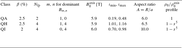
given in table 1.
For each equilibrium, the shear-Alfvén continuum and Alfvén vorticity eigenproblems are calculated using the STELLGAP (Spong et al. Reference Spong, Sanchez and Weller2003) and AE3D (Spong et al. Reference Spong, D’azevedo and Todo2010) codes. The transport of the fusion-born alpha particle distribution, consistent with reactivity (2.8), is modelled using Monte Carlo simulations for various perturbation amplitudes, identifying the mode amplitude necessary to drive prompt fast ion losses.
Summary of stellarator equilibria parameters scaled to ARIES-CS size.

Table 1 Long description
A table comparing stellarator equilibria parameters scaled to ARIES-CS size. The table has six columns and three rows. The columns are labeled Class, β (percent), N_fp, m, n for dominant B_m,n, B_0^axis (T), t_min, t_max, Aspect ratio A = R/a, and ρ_0/ρ_0^axis profile. The rows are labeled QA, QH, and QI. Row 1: Class, QA; β (percent), 2.5; N_fp, 2; m, 1; n for dominant B_m,n, 0; B_0^axis (T), 5.9; t_min, 0.19; t_max, 0.48; Aspect ratio A = R/a, 6.0; ρ_0/ρ_0^axis profile, 1. Row 2: Class, QH; β (percent), 2.5; N_fp, 4; m, 1; n for dominant B_m,n, 4; B_0^axis (T), 5.9; t_min, 1.01; t_max, 1.16; Aspect ratio A = R/a, 6.5; ρ_0/ρ_0^axis profile, 1 - s^5. Row 3: Class, QI; β (percent), 2; N_fp, 4; m, 0; n for dominant B_m,n, 4; B_0^axis (T), 6.0; t_min, 0.70; t_max, 0.98; Aspect ratio A = R/a, 10.0; ρ_0/ρ_0^axis profile, 1 - s^5.
For QA and QH equilibria, we consider
 $\beta =2.5\,\%$
equilibria from Landreman et al. (Reference Landreman, Buller and Drevlak2022) as representative cases. For QI equilibrium, we consider a
 $\beta =2\,\%$
equilibrium Stable Quasi-Isodynamic Design similar to Goodman et al. (Reference Goodman, Xanthopoulos, Plunk, Smith, Nührenberg, Beidler, Henneberg, Roberg-Clark, Drevlak and Helander2024). On each flux surface, the equilibrium
 $B_0$
field strength of these equilibria is represented as a superposition of QS harmonics
 $B_{m,n}(m\theta -n\zeta )$
, summed over integers
 $m$
and
 $n$
. Although none of the equilibria are exactly QS, each has a dominant
 $B_{m,n}$
component across the entire volume. The
 $m$
and
 $n$
values of the dominant
 $B_{m,n}$
for each equilibrium are summarised in table 1. Notably, the on-axis thermal pressure corresponding to the profiles from Bader et al. (Reference Bader, Anderson, Drevlak, Faber, Hegna, Henneberg, Landreman, Schmitt, Suzuki and Ware2021) used here is twice the value targeted in the QH optimisation (Landreman et al. Reference Landreman, Buller and Drevlak2022), but this inconsistency does not affect the conclusions below, so we retain the original profiles and equilibria for ease of reference.
Alfvén continuum (left) and radially global SAW eigenfunctions (right) for QA (top, 30.3 kHz) and QI (bottom, 46.8 kHz) configurations from table 1, computed with STELLGAP and AE3D. Black dots indicate mode amplitude maxima; red squares mark the highlighted global modes. As in figure 1, coloured lines show the five Fourier harmonics (2.5) with the largest peak
 $\varPhi _{m,n}$
amplitude, with
 $m$
and
 $n$
mode numbers labelled in the legend. Grey lines show the remaining lower-amplitude harmonics from the simulation. The narrow gaps in QA lead to strong continuum damping in the presence of the density shear, whereas the wide helical gaps in QI support radially extended global SAW that persist despite the edge continuum shear near
 $s \sim 1$
caused by the
 $\rho _0^{\mathrm{axis}}(1-s^5)$
density profile.

The STELLGAP Alfvén continuum calculations, and the global SAWs from AE3D for equilibria in table 1 are shown in figure 1 for QH, and in figure 2 for QA and QI stellarators. Dynamic mode resolution parameters for all simulations are outlined in Appendix A. Note that the sheared
 $\rho _0^{\mathrm{axis}}(1-s^5)$
density profile used in QH and QI equilibria results in steepening near the edge
 $s\sim 1$
, characteristic of the Alfvén velocity profile shear
 $v_{A}^2\sim B_0^2/\rho _0$
due to a decrease in plasma density
 $\rho _0$
near the last flux surfaces. Accordingly, the radially global SAWs residing in the continuum frequency gaps have most of their energy localised away from the device edge.
Due to much narrower frequency gaps in the QA continuum compared with QH and QI continua shown in figures 1 and 2, the QA equilibrium modes are more sensitive to continuum damping induced by the density shear. For the QI and the QH equilibria, AE3D finds global modes that persist in both flat and sheared
 $\rho _0^{\mathrm{axis}}(1-s^5)$
plasma density profiles, with radial structure unaffected by the difference in Alfvén velocity shear in these two cases. For the QA equilibria, none of the radially global modes found in flat profiles persisted in the sheared
 $\rho _0^{\mathrm{axis}}(1-s^5)$
density profile because of the continuum damping near the edge. This supports continuum gap width optimisation (Paul et al. Reference Paul, Hyder, Rodríguez, Jorge and Knyazev2025) as a viable strategy for SAW suppression. In the case of a flat density profile, radial Alfvén velocity shear comes from the variation in the magnetic field strength
 $B_0$
, and the overall shear is decreased relative to the
 $\rho _0^{\mathrm{axis}}(1-s^5)$
profile. We find a SAW in the QA configuration with a flat density profile, and use it in our analysis. Notably, radial scales of SAWs in figures 1 and 2 are larger than the characteristic drift orbit width for corresponding equilibria, which is the expected (Gorelenkov, Pinches & Toi Reference Gorelenkov, Pinches and Toi2014) radial scale for the most efficiently driven modes. Indeed, for QA in table 1, the passing and trapped orbits have characteristic widths (Paul et al. Reference Paul, Bhattacharjee, Landreman, Alex, Velasco and Nies2022)
 $\varDelta _{\mathrm{pass}} / a = r_\alpha /(\iota a)\sim 0.08$
and
 $\varDelta _{\mathrm{tr}} / a =\sqrt {A}r_\alpha /(\iota a)\sim 0.2$
, respectively, where
 $r_\alpha \sim \,4.5\,{\mathrm{cm}}$
is the approximate Larmor radius of alpha particles. For a QH equilibrium field
 $B_0(s,\chi =M\theta -N\zeta )$
, orbits are narrower by a factor
 $\sim 1/|M\iota -N|$
, and for QI the orbit width
 $\sim |I|/a$
vanishes in the vacuum limit. This suggests that fusion-born alphas most efficiently drive SAWs at higher poloidal mode numbers than those obtained with the minimal model (2.3), particularly for QH and QI. Additionally, as reactivity profile (2.8) peaks near the axis
 $s\lt 0.2$
, waves driven by fusion-born alphas would likely be localised deeper in the plasma core than the SAWs in figures 1 and 2.
The figure compares equilibrium fields and losses for QA (dotted), QH (solid) and QI (dashed) stellarators from table 1. Left panel shows (black) dominant Boozer harmonics
 $B_{M,N}$
and (red) mirror ratio
 $B_{\max }/B_{\min }$
. The right three panels show prompt losses in QA, QH and QI equilibria, for passing (blue circles), trapped (green squares) and barely trapped (red triangles) orbit classes. Black diamond lines show total losses across orbit classes. Grey dash-dotted lines show losses without SAW. Without SAW, the fractions of passing (barely trapped) particles are
 $83.3\,\%$
(
 $3.4\,\%$
) for QA,
 $71.3\,\%$
(
 $2.5\,\%$
) for QH and
 $58.6\,\%$
(
 $0.8\,\%$
) for QI, with the rest of the particles in the ‘other trapped’ category.

Figure 3. Long description
The figure contains four panels. Panel A shows a line graph comparing the dominant Boozer harmonics (B M,N) in Tesla on the left y-axis and the mirror ratio (B max/B min) on the right y-axis against the variable s on the x-axis. The lines represent different stellarators: QA (dotted), QH (solid), and QI (dashed). Panel B shows a scatter plot of the loss fraction per orbit class for the QA stellarator, with passing particles in blue circles, trapped particles in green squares, barely trapped particles in red triangles, and total losses in black diamonds. The x-axis represents the square root of delta U/U 0 times 10 to the power of 3, and the y-axis is on a logarithmic scale. Panel C shows a similar scatter plot for the QH stellarator. Panel D shows a similar scatter plot for the QI stellarator. Each panel includes a grey dash-dotted line indicating losses without shear-Alfvén wave (SAW) perturbations.
The rest of the section will use the equilibria and global SAWs described above to illustrate and verify the analysis. Although the SAWs shown in figures 1 and 2 are representative of radially global waves we find for equilibria in table 1 with vorticity model (2.3), different SAWs can generally lead to quantitatively different transport, so impact from all unstable SAWs should ideally be considered for transport modelling. We characterise the magnitude of SAW perturbation by the magnetic field energy ratio between the wave
 $\delta U\!$
and the equilibrium
 $U_0$
 \begin{align} \frac {\delta U}{U_0}=\frac {\int \mathrm{d}^3\boldsymbol{r} \delta B^2}{\int \mathrm{d}^3\boldsymbol{r} B_0^2}. \end{align}
As energy is quadratic in wave amplitude,
 $\sqrt {\delta U/U_0}$
serves as a measure for average magnetic field perturbation in stellarator volume. Another common (Nazikian et al. Reference Nazikian1997; Paul et al. Reference Paul, Mynick and Bhattacharjee2023) way to characterise SAW amplitude is the normalised maximum of the magnetic field perturbation
 \begin{align} \delta \hat B^s=\frac {\delta \boldsymbol{B}\boldsymbol{\cdot }\boldsymbol{\nabla }s}{B_0|\boldsymbol{\nabla }s|}. \end{align}
For the SAWs and equilibria we consider, prompt losses for different wave amplitudes
 $\sqrt {\delta U/U_0}$
are shown in figure 3. Measured prompt EP losses exceed 1 % for the medium
 $\sqrt {\delta U/U_0}$
(maximum radial (3.2)) magnetic field of
 $1\times 10^{-3}$
(
 $3.1\times 10^{-3}$
) in QA,
 $2.15\times 10^{-3}$
(
 $6.6\times 10^{-3}$
) in QH and
 $2.15\times 10^{-3}$
(
 $3.3\times 10^{-3}$
) in QI. This is consistent with the
 $2\times 10^{-3}$
threshold reported for the Tokamak Fusion Test Reactor (TFTR) (Hsu & Sigmar Reference Hsu and Sigmar1992). Notably, threshold magnetic fields across fusion-relevant tokamak analyses vary significantly, with TFTR experiments (Nazikian et al. Reference Nazikian1997) reporting prompt losses with inferred normalised field amplitudes of
 $\delta \hat B^s\sim 10^{-5}$
, while recent prompt loss analysis for the International Thermonuclear Experimental Reactor (Van Zeeland et al. Reference Van Zeeland2012) suggests negligible losses for amplitudes up to
 $\delta \hat B^s\sim 10^{-3}$
. Experiments from the Large Helical Device (LHD) (Ogawa et al. Reference Ogawa, Isobe, Toi, Spong and Osakabe2012) observe prompt losses for similar
 $\delta \hat B^s\sim 10^{-4}{-}10^{-3}$
inferred SAW amplitudes.
3.1. Passing resonance analysis for single harmonic SAW
To better understand the onset of stochastic transport caused by the presence of the SAW, it is instructive to consider the simplest case of a precisely QS equilibrium with a perturbation mode consisting of a single Fourier harmonic
 $(m,n)$
in Boozer coordinates. Under these assumptions, the dynamics of a passing particle in a stellarator can be analysed similarly to the tokamak case (Mynick Reference Mynick1993), as was done (Paul et al. Reference Paul, Mynick and Bhattacharjee2023) to show that the field-strength helicity of QH equilibria suppresses stochastic transport. In what follows, we generalise the analysis done in Paul et al. (Reference Paul, Mynick and Bhattacharjee2023) to the case of arbitrary helicity symmetry. The extended analysis includes the QP case, which is appropriate for approximating QI equilibria.
The resonant analysis below relies on several assumptions regarding equilibrium unperturbed particle dynamics and the perturbation field:
-
(i) Quasi-symmetric magnetic field: the equilibrium magnetic field is assumed to be QS, i.e.
 $B_0(s,\theta ,\zeta )=B_0(s,\chi =M\theta -N\zeta )$
, where
$M$
and
$N$
are integers specifying the field helicity. Current techniques of stellarator optimisation (Landreman & Paul Reference Landreman and Paul2022) achieve sufficient quasi-symmetry precision to justify this assumption. This analysis can also be useful for QI equilibria that can be approximated by QP symmetry.
-
(ii) Single harmonic perturbation: similar to the earlier works (Mynick Reference Mynick1993; Paul et al. Reference Paul, Mynick and Bhattacharjee2023), the perturbation is taken as a single Fourier harmonic, which provides continuous symmetry in the problem and a resulting motion invariant. This motion invariance is absent in SAWs consisting of several Fourier harmonics in Boozer coordinates, which significantly complicates the analysis (White Reference White2012).
-
(iii) Passing particle assumption: for passing particles, we can express the unperturbed motion as a Fourier series in the symmetry angle
$\chi$
for the resonance analysis (see Appendix B for details). The same approach does not work for trapped particles that have consecutive bounces
$\Delta \chi _{\mathrm{b}}$
in the same field period
$\Delta \chi _{\mathrm{b}}\lt 2\pi$
. However, our conclusions will still hold for barely trapped particles
$\Delta \chi _{\mathrm{b}}\gg 2\pi$
. Notably, passing particles also have a one-to-one correspondence between the particle’s energy
$E$
and its parallel velocity
$v_{\|}$
. This enables one to construct Poincaré cross-sections of perturbed EP motion, discussed in § 3.2.1, to verify our resonance analysis, as shown in figure 4. -
(iv) Single Fourier harmonic in unperturbed trajectory: for passing particles (assumption iii), we further assume that the Fourier expansion of the trajectory in the symmetry angle
$\chi$
has a single dominant harmonic. This is consistent with QA and QH equilibria: the near-axis (Landreman & Sengupta Reference Landreman and Sengupta2018) expansion(3.3)guarantees a single dominant field-strength Fourier harmonic near the axis, and the corresponding
\begin{align} B_0(s,\chi )= B_0^{\mathrm{axis}}(1-\bar \xi \sqrt {s} \cos (\chi )),\quad \bar \xi =const, \end{align}
$\boldsymbol{\nabla }B_0$
drift then produces a dominant Fourier harmonic in the particle’s trajectory. Although the same near-axis expansion (3.3) does not apply to QI equilibria, they can still have a dominant harmonic in Boozer components. One such example is the QI equilibrium considered in table 1, where a single poloidal
$M=0$
harmonic dominates equilibrium field
$B_0$
across the stellarator volume, as illustrated in figure 3.
-
(v) Lastly, for simplicity, we consider a vacuum
$I=0$
field. This is consistent with the low-
$\beta$
assumption and the near-axis expansion of stellarator equilibrium.


The figure shows interaction between a single harmonic SAW and passing
 $\mu =0$
alpha particles co-propagating along the QP approximation to the QI field. The QI equilibrium is described in table 1. The perturbation is the most energetic harmonic of the
 $\omega =46.8\,{\mathrm{kHz}}$
SAW in the QI equilibrium, with poloidal
 $m=15$
and toroidal
 $n=16$
mode numbers. Left panel demonstrates resonance analysis (3.10), showing that the mode resonates with the co-propagating trajectory of helicity
 $h=0.933$
near
 $s=0.905$
flux surface. This agrees with the Poincaré cross-section shown in the right panel, where there is an island chain at
 $s=0.905$
. The middle panel shows the radial profile
 $\varPhi _{15,16}(s)$
of the mode, with zero crossings
 $\varPhi _{15,16}=0$
creating ‘island-like’ structure on the Poincaré map. Because of the wide spacing between
 $l=0$
and
 $l=1$
resonances, the island overlap is avoided for this perturbation.

Figure 4. Long description
The figure contains three panels: Panel A, Panel B, and Panel C. Panel A is a line graph showing resonance analysis. The horizontal axis is labeled h with units of omega theta over omega zeta, ranging from 0.7 to 1.0. The vertical axis is labeled s, ranging from 0 to 1.0. The graph includes lines representing co-propagating and counter-propagating trajectories with different helicity values. Panel B is a line graph showing the radial profile of the mode. The horizontal axis is labeled Phi 15 16 with units of volts, ranging from 0 to 2. The vertical axis is unlabeled but shows a sinusoidal pattern. Panel C is a Poincaré cross-section plot. The horizontal axis is labeled chi over pi, ranging from 0 to 2. The vertical axis is unlabeled but shows an island chain structure. The color bar on the right indicates digit accuracy, ranging from 0 to 7. The graphs collectively illustrate the resonance and stability of shear-Alfvén waves in the presence of energetic particles.
Under the listed (i–v) assumptions, it can be shown (see Appendix B) that the
 $(m,n)$
SAW harmonic of frequency
 $\omega$
resonates with the unperturbed drift orbit when
 \begin{align} \varOmega _{l}&= \omega +(m+lM)\omega _\theta -(n+lN)\omega _\zeta =0. \end{align}
This resonance condition (3.4) can be expressed in terms of orbit helicity
 $h=\omega _\theta /\omega _\zeta$
as
 \begin{align} h_l = \frac {n+lN-\omega /\omega _\zeta }{m+lM}, \end{align}
where
 $l$
is the integer describing the drift harmonic,
 $h_l$
is the corresponding resonant helicity and
 $\omega _\theta$
(
 $\omega _\zeta$
) is the time-averaged drift in poloidal (toroidal) Boozer angle
 \begin{align} \omega _\theta =\lim _{T\to \infty }\int _0^T\frac {\dot \theta {\rm d}t}{T}, \quad \omega _\zeta =\lim _{T\to \infty }\int _0^T\frac {\dot \zeta {\rm d}t}{T}. \end{align}
Neglecting (Paul et al. Reference Paul, Mynick and Bhattacharjee2023) radial dependence of the average toroidal drift,
 ${\rm d}\omega _\zeta /{\rm d}s=0$
, the island width at the resonant (3.5) helicity
 $h_l$
has radial width
 \begin{align} w_l^s\approx \sqrt {\frac {s_l}{(m+lM){\rm d}\omega _\theta /{\rm d}s}}, \end{align}
where
 $s_l$
is the radial drift amplitude (see (B8) in Appendix B). It follows from (3.5) that the spacing between the neighbouring resonance helicities
 $h_l$
and
 $h_{l+1}=h_l-\Delta s_l ({\rm d}h_l/{\rm d}s)$
is
 \begin{align} \Delta s_l=\frac {1}{{\rm d}h_l/{\rm d}s}\frac {Mh_0-N}{m+(l+1)M}. \end{align}
Comparing the width
 $w_l^s$
of resonance islands (3.7) with the spacing
 $\Delta s_l$
between resonances (3.8) gives the island overlap condition (Chirikov Reference Chirikov1971) for the stochasticity onset
 \begin{align} \frac {w_l^s}{\Delta s_l}=\frac {m+(l+1)M}{(Mh_0-N)\omega _\zeta } \sqrt {\left |\frac {s_l}{m+lM}\frac {{\rm d}\omega _\theta }{{\rm d}s}\right |}\gtrsim 1. \end{align}
For a QH equilibrium,
 $\chi _{\mathrm{QH}}=\theta -N\zeta$
, the stochasticity threshold criterion (3.9) recovers results obtained in Paul et al. (Reference Paul, Mynick and Bhattacharjee2023). For a QP case,
 $\chi _{\mathrm{QP}}=-N\zeta$
, the resonance condition (3.4) is
 \begin{align} \varOmega _{l,{\mathrm{QP}}}=\omega +m\omega _\theta -(n+lN)\omega _\zeta =0, \end{align}
which corresponds (3.5) to helicity
 \begin{align} h_{\mathrm{QP}}=\frac {n+lN-\omega /\omega _\zeta }{m}. \end{align}
The corresponding stochasticity threshold (3.9) for QP is
 \begin{align} \frac {w_{l,{\mathrm{QP}}}^s}{\Delta s_{l,{\mathrm{QP}}}}=-\frac {m}{N\omega _\zeta }\sqrt {\left |\frac {s_l}{m}\frac {{\rm d}\omega _\theta }{{\rm d} s}\right |}\gtrsim 1. \end{align}
As in the QH case, stochasticity is suppressed for large
 $N$
. This corresponds to a poloidally symmetric field with a larger number of field periods
 $N_{\mathrm{fp}}$
. Notably, QP has wider spacing between resonant islands (3.8) than QH with the same sign of
 $Mh_0$
and
 $N$
, leading (3.9) to stochasticity suppression. The resonance (3.10) with
 $m=0$
modes no longer depends on
 $\omega _\theta$
: it occurs when
 $\omega /\omega _\zeta =n-lN$
. In this case, the stochasticity onset is determined not by poloidal
 ${\rm d}\omega _\theta /{\rm d}s$
as in (3.12) but rather toroidal
 ${\rm d}\omega _\zeta /{\rm d}s$
shear.
3.1.1. Orbit classification and passing–trapped transitions
When the particle mirrors in a precisely QS field, consecutive bounces remain within the same period of the field symmetry angle,
 $\Delta \chi _{\mathrm{b}} \lt 2\pi$
. However, SAW perturbations cause radial displacement away from the initial flux surface. A different peak magnetic field strength
 $B_0^{\mathrm{max}}$
at that new location means that a particle that is passing in the unperturbed field can mirror in the presence of SAW even after several periods,
 $\Delta \chi _{\mathrm{b}} \gt 2\pi$
. This wave-induced transition between passing and barely trapped orbit classes can lead to prompt losses (Hsu & Sigmar Reference Hsu and Sigmar1992). This loss channel is more pronounced for equilibria with larger radial variation in the mirror ratio. Notably, while it follows from the near-axis QS expansion (3.3) that the QA and QH equilibria always have significant radial variation in their dominant
 $B$
harmonic, the radial variation of the magnetic field strength in QI is typically (Velasco et al. Reference Velasco, Calvo, Sánchez and Parra2023) small. This difference in radial
 $B_0$
variation is illustrated in figure 3 and suggests that the transition between passing and trapped orbit classes is more pronounced in QA and QH than in QI. We test this numerically by considering (Paul et al. Reference Paul, Bhattacharjee, Landreman, Alex, Velasco and Nies2022) the change in the symmetry angle
 $\chi$
between bounces of each lost particle: the passing particle never bounces, the ‘barely trapped’ particles travel over a
 $2\pi$
period in
 $\chi$
between bouncing and the remaining losses are particles trapped in the main harmonic of the field strength. For QI, we use the QP symmetry angle
 $\chi =-N\zeta$
for orbit classification. Consistent with this analysis, figure 3 shows that in QS equilibria, significant SAW-induced losses occur for ‘barely trapped’ orbits. This is similar to the SAW-induced orbit transition loss mechanism in tokamaks (Hsu & Sigmar Reference Hsu and Sigmar1992). Due to the lower radial variance in magnetic field strength, this mechanism is suppressed in QI. Consistent with the resonant analysis (3.9), passing particle losses are suppressed in QH and QI because field periods
 $N_{\mathrm{fp}}$
in these cases increase helicity
 $N$
. Notably, the majority of losses in QI come from trapped particles. This motivates future work on extending resonant analysis beyond passing particles.
3.2. Stochastic motion identification
For identifying island overlap and stochasticity onset under assumptions of § 3.1, we can use Poincaré cross-section technique described in § 3.2.1. However, the assumptions (i–iii) required to construct Poincaré cross-sections are too restrictive for comprehensive transport assessment. For a general trajectory, we measure stochasticity using weighted Birkhoff averaging technique described in § 3.2.2.
3.2.1. Kinetic Poincaré cross-sections
Under assumptions (i–iii) from the resonance analysis in § 3.1, it is possible to construct (Paul et al. Reference Paul, Mynick and Bhattacharjee2023) a kinetic Poincaré cross-sections for perturbed particle motion.
For constructing the Poincaré cross-section, note that the Boozer angle dependence of the SAW phase can be expressed in terms of the symmetry angle
 $\chi$
and some other angle
 $\eta =M_\eta \theta +N_\eta \zeta$
, with
 $M_\eta$
and
 $N_\eta$
such that
 $s,\chi ,\eta$
form a valid coordinate system. For precisely QS field, Lagrangian (2.1) becomes a function of
 $L(s,\chi ,n_\eta \eta -\omega t,v_\|)$
, where
 $n_\eta =(mN-nM)/(MN_\eta -M_\eta N)$
. Therefore,
 \begin{align} n_\eta \frac {\partial L}{\partial t}+\omega \frac {\partial L}{\partial \eta } = \frac {\rm d}{{\rm d}t}(n_\eta E-\omega P_\eta )=0, \end{align}
where
 \begin{align} E=\frac {M_{\mathrm{s}}v_\|^2}{2} +\mu B_0 + q_{\mathrm{s}}\delta \varPhi \end{align}
is the energy and
 \begin{align} P_\eta =\frac {\partial L}{\partial \dot \eta }=\frac {q_{\mathrm{s}}[(M\psi _{\mathrm{p}}-N \psi )-\alpha (NI+MG)]}{MN_\eta -M_\eta N}-\frac {M_{\mathrm{s}} v_\|(NI+MG) }{B_0(MN_\eta -M_\eta N)} \end{align}
is the canonical momentum conjugate to
 $\eta$
. For fixed
 $n_\eta \eta -\omega t=\bar \eta =\mathrm{const}$
, integral of motion (3.13) gives a quadratic equation for
 $v_\|$
in terms of
 $\mu$
,
 $s$
,
 $\chi$
and
 $\bar \eta$
. Since passing particles do not bounce, they preserve the sign of
 $v_\|$
, so
 $v_\|$
can be determined (3.13) from values of
 $\mu ,\,E'=n_\eta E-\omega P_\eta ,\,\chi$
and
 $s$
. This allows one to construct Poincaré cross-section for passing particles of the same
 $\mu$
,
 $E'$
values by recording their
 $s$
and
 $\chi$
values at fixed
 $\bar \eta$
, as shown in figure 4.
Poincaré cross-sections allow study of the resonances described by (3.4) and illuminate the impact of radial mode amplitude dependence
 $\varPhi _{m,n}(s)$
on fast ion drift surfaces. An example in figure 4 shows drift surface deformation caused by the interaction with the mode. First is the resonance with the mode (3.4) described in the previous section. The second mechanism, also producing the island-like structures on the Poincaré map, is associated with the radial sign reversal of the wave’s electric
 $\delta \boldsymbol{E}$
and magnetic
 $\boldsymbol{\delta B}$
fields. Recall that the wave’s contribution to the EP radial
 $\delta s$
dynamics (2.1) is because the (a) electric field of the mode causes radial
 $\boldsymbol{\delta E}\times \boldsymbol{B}_0$
drift and (b) the radial component of
 $\delta B$
displaces field lines from equilibrium flux surfaces
 $s=\mathrm{const}$
,
 $\boldsymbol{B}\boldsymbol{\cdot }\boldsymbol{\nabla }s = \boldsymbol{\delta B}\boldsymbol{\cdot }\boldsymbol{\nabla }s$
, causing particles streaming along field lines to drift radially. For a single harmonic SAW, these two effects are given by
 \begin{align} \delta \dot s=-\left (1+(\iota m -n)\frac {v_{\|}B_0}{\omega G}\right )\frac {m}{q_{\mathrm{s}}\psi _0}\varPhi _{m,n}(s)\sin (m_\chi \chi - \bar \eta ), \end{align}
where
 $m_\chi =(mN_\eta -nM_\eta )/(MN_\eta -M_\eta N)$
. Near the radial location where
 $\varPhi _{m,n}(s)=0$
, the wave-induced
 $\boldsymbol{E}\times \boldsymbol{B}$
drifts on either side of the zero have opposite directions. Similarly,
 $\delta \boldsymbol{B}$
is also oppositely directed there. The result is the island-like deformation of the drift surfaces near radial locations of zero wave amplitude. Figure 4 also shows that ‘island-like’ chains for neighbouring
 $\varPhi _{m,n}(s)=0$
zeros are shifted in by
 $m_\chi \chi \sim \pi$
relative to each other, corresponding to changes in radial
 ${\rm d}\varPhi _{m,n}/{\rm d}s$
slope.
3.2.2. Weighted Birkhoff averaging
Another useful technique for assessment of particle’s motion stochasticity is the recently proposed (Duignan & Meiss Reference Duignan and Meiss2023) weighted Birkhoff averaging (WBA) method. Unlike the Poincaré cross-section technique, the WBA approach does not rely on any of the (i–iii) assumptions, making it suitable for analysing SAW-induced stochasticity for all particles in non-QS equilibria with general Alfvén wave perturbations.
In this work, we consider WBA of the canonical momentum
 $P_\eta$
over a trajectory of duration
 $t_{\mathrm{traj}}$
, defined as
 \begin{equation} \mathrm{WBA}_{t_{\mathrm{traj}}}(P_\eta ) = \frac {1}{t_{\mathrm{traj}}}\int _0^{t_{\mathrm{traj}}} C\,e^{-[{{t}/{t_{\mathrm{traj}}}(1-({t}/{t_{\mathrm{traj}}}))}]^{-1}} P_\eta (t)\,\mathrm{d}t, \end{equation}
where
 $C$
is a normalisation constant. The infinitely differentiable bump function in (3.17) vanishes at the endpoints, and provides super-polynomial convergence of the average for quasi-periodic orbits (Duignan & Meiss Reference Duignan and Meiss2023). For chaotic orbits the convergence is comparatively slow and is at best polynomial in
 $t_{\mathrm{traj}}$
. The digit accuracy,
 \begin{align} \mathrm{DA}_{t_{\mathrm{traj}}} = -\log _{10}\!\left (2\frac {\left |\mathrm{WBA}_{{t_{\mathrm{traj}}}/2}(P_\eta ) - \mathrm{WBA}_{t_{\mathrm{traj}}}(P_\eta )\right |}{\left |\mathrm{WBA}_{{t_{\mathrm{traj}}}/2}(P_\eta )\right |+\left |\mathrm{WBA}_{t_{\mathrm{traj}}}(P_\eta )\right |}\right )\!, \end{align}
quantifies this convergence rate by comparing the averages computed over the first half and the full trajectory (Lachmann, Knyazev & Paul Reference Lachmann, Knyazev and Paul2026). High DA values correspond to rapid convergence and identify regular motion, while lower DA values identify stochastic orbits. Accordingly, the motion is classified as stochastic when its
 $\mathrm{DA}$
is below the threshold
 $\mathrm{DA}=\mathrm{DA_{threshold}}$
value. To find a suitable threshold
 $\mathrm{DA_{threshold}}$
value, it is instructive to evaluate
 $\mathrm{DA}$
on a Poincaré cross-section, as illustrated in figure 4. Note that choosing
 $\eta$
such that
 $P_\eta$
is an approximate invariant of the system can lead to better distinction (Duignan & Meiss Reference Duignan and Meiss2023) in the convergence rate of DA for regular and stochastic motions, but the existence of such an approximate invariant is not required for the method. For the WBA calculation (3.17) in QI and its QP approximation shown in figure 4, we choose
 $\eta$
to be
 $\theta$
, while for the QS configurations in table 1 we choose
 $\eta$
to be
 $\zeta$
. Although the computed value of DA can depend on implementation details (Ruth & Bindel Reference Ruth and Bindel2024), such as the filtering function or numerical scheme used for modelling the particle dynamics, analysis of FIRM3D tracing results (Lachmann et al. Reference Lachmann, Knyazev and Paul2026) shows
 $\mathrm{ DA_{threshold}}=3$
is a suitable classification threshold across configurations and perturbation amplitudes we consider.
For assessment of SAW-induced stochasticity of different orbit classes, it is instructive to compute their fraction of low
 $\mathrm{DA}\lt \mathrm{DA}_{\mathrm{threshold}}$
particles (Lachmann et al. Reference Lachmann, Knyazev and Paul2026). For each stellarator from table 1, we trace 5000 fusion-born alpha particles, classify them by orbit type and compute their digit accuracy. Resulting stochastic fractions for different SAW amplitudes are shown in figure 5.
Three panels show the fraction of low digit accuracy
 $\mathrm{DA}\lt \mathrm{DA_{threshold}}=3$
fusion-born alpha particles in QA (left), QH (centre) and QI (right) equilibria, for passing (blue circles), trapped (green squares) and barely trapped (red triangles) orbit classes. Black diamond lines show total fraction across orbit classes.

In the absence of SAW perturbations, the WBA analysis in figure 5 shows that most stochastic particles are trapped. This is consistent with recent analysis of phase-space integrability in QS stellarators (Chambliss, Paul & Hudson Reference Chambliss, Paul and Hudson2025), which showed that trapped drift orbits are more susceptible to resonances with symmetry-breaking equilibrium perturbations than passing orbits. Notably, for sufficiently large SAW perturbations, the fraction of stochastic passing orbits exceeds that of trapped orbits. This suggests that, in contrast to the equilibrium perturbations considered in Chambliss et al. (Reference Chambliss, Paul and Hudson2025), time-dependent SAW perturbations primarily resonate with passing orbits, consistent with the resonance analysis of § 3.1.
For passing orbits, the stochastic fraction in the four-field-period
 $(N_{\mathrm{fp}}=4)$
QH and QI cases is lower than in QA. This agrees with the resonance analysis of § 3.1, where the increase in field helicity
 $N$
is shown to suppress island overlap (3.9) in QH and QI but not QA. However, the island overlap condition does not account for the radial mode structure or the differences in dominant harmonic composition (2.5) between SAW in different equilibria. As shown in figures 1 and 2, SAW modes can differ significantly across stellarators, complicating direct stochasticity comparisons. We note, for example, that while the resonance analysis predicts wider island spacing (3.8) in the QI case than in QH for the same perturbation harmonic, figure 5 shows no reduction in the stochastic passing orbit fraction for QI relative to QH.
Since stochasticity only leads to prompt losses when the stochastic region intersects the last closed flux surface, it is possible to have a large stochastic fraction with small prompt losses. For example, figure 5 shows a large fraction of stochastic passing particles in the QH case for perturbations with average amplitude
 $\sqrt {\delta U/U_0}\gtrsim 10^{-4}$
, yet figure 3 shows that these particles do not contribute to prompt losses until the larger amplitude
 $\sqrt {\delta U/U_0}\gtrsim 10^{-3}$
. This is especially relevant for SAW perturbations localised away from the edge due to radial Alfvén velocity shear, as discussed in § 3.
Consistent with the orbit classification analysis of § 3.1.1, figure 5 shows that QA and QH have a larger stochastic fraction of barely trapped particles than QI, due to the larger radial variance in magnetic field strength illustrated in figure 3. Despite the suppressed barely trapped stochastic fraction in QI, figures 3 and 5 show significant stochastic prompt losses from trapped orbits in both QI and QH cases. Further work is needed to generalise the stochasticity-onset criterion (3.9) beyond passing orbits.
4. Conclusion
We extend the resonance analysis of Paul et al. (Reference Paul, Mynick and Bhattacharjee2023) to SAWs consistent with equilibrium field and Alfvén velocity profiles, and show that these perturbations drive significant prompt alpha particle losses in optimised QA, QH and QI stellarators at amplitudes
 $\delta \hat {B}_s \sim 10^{-3}$
consistent with observations in LHD (Ogawa et al. Reference Ogawa, Isobe, Toi, Spong and Osakabe2012) and TFTR (Hsu & Sigmar Reference Hsu and Sigmar1992).
The resonance analysis for passing particles shows that increased field helicity
 $N$
widens the spacing between resonant islands in QH and QI but not QA, suppressing wave-induced stochastic transport in the former two cases. Notably, this suppression is not specific to SAW perturbations and applies to any transverse electromagnetic perturbation resonant with the passing particle drift motion. The passing resonance analysis also extends to barely trapped particles. We show that, because of reduced radial variation in magnetic field strength in QI, SAW-induced orbit-class transitions are suppressed in QI relative to QA and QH stellarators.
The resonance analysis is verified with kinetic Poincaré cross-sections and WBA (Duignan & Meiss Reference Duignan and Meiss2023; Lachmann et al. Reference Lachmann, Knyazev and Paul2026) diagnostics implemented in the FIRM3D code (Paul et al. Reference Paul, Knyazev, Czekanski, Lachmann, Hyder, Albert and Landreman2026). We note, however, that the resonance analysis does not account for radial variation in wave amplitude, which can independently structure transport, as illustrated by the island-like features in the Poincaré cross-sections near
 $\varPhi _{m,n}(s) = 0$
. Radial amplitude variation is expected for SAWs, since Alfvén velocity shear from plasma density profiles induces shear in the Alfvén continuum and promotes continuum damping. This effect is particularly pronounced in QA case we considered, where narrow frequency gaps cause global modes to be fully damped under the
 $\rho _0^{\mathrm{axis}}(1-s^5)$
density shear, whereas radially global SAWs persist in QH and QI under the same shear due to wider gaps. This supports continuum gap optimisation (Paul et al. Reference Paul, Hyder, Rodríguez, Jorge and Knyazev2025) as a viable approach to SAW-induced transport suppression. We also note that differences in harmonic composition of SAW eigenmodes across configurations complicate direct stochasticity comparisons between them.
Stochasticity analysis with WBA and loss fraction calculations show significant stochastic transport of trapped particles driven by SAW perturbations, motivating future extension of the resonance analysis beyond passing orbits. Notably, even when the stochastic phase-space region does not intersect the last closed flux surface, stochastic transport can redistribute fast ions. The evolution of the profiles under the imposed SAW perturbation can be studied with the minimal model described in this work. A more complete transport assessment would require evolving the SAW self-consistently with the distribution function. Such an analysis can be done with quasilinear (Gorelenkov et al. Reference Gorelenkov, Duarte, Podesta and Berk2018) or nonlinear models, and is important for assessing EP transport in stellarator FPP designs.
Acknowledgements
Editor Per Helander thanks the referees for their advice in evaluating this article.
Funding
We acknowledge funding through the U.S. Department of Energy, under contracts DE-SC0024630, DE-SC0024548 and DE-AC02-09CH11466. We also acknowledge funding through the Simons Foundation collaboration ‘Hidden Symmetries and Fusion Energy’, Grant No. 601958. This research used resources of the National Energy Research Scientific Computing Center (NERSC), a Department of Energy Office of Science User Facility using NERSC award ERCAP0031926.
Declaration of interests
The authors report no conflict of interest.
Data availability statement
The data and scripts that reproduce the figures in this paper are openly available on Zenodo at https://doi.org/10.5281/zenodo.21299907.
Appendix A. STELLGAP and AE3D harmonic resolution
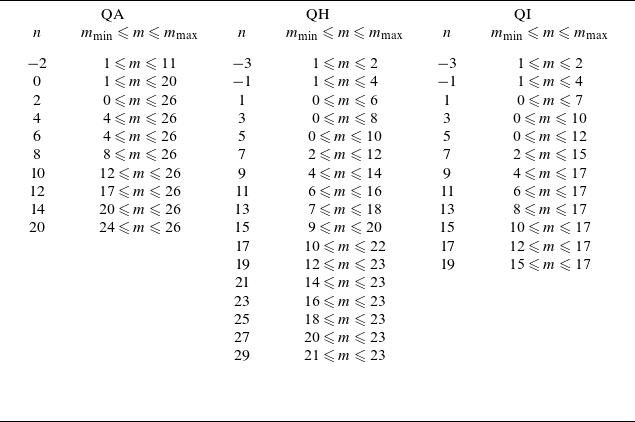
We used the STELLGAP and AE3D codes to calculate the Alfvén continua and radially global SAWs for this study. Both codes represent a SAW as a superposition of cosine terms in Boozer angles. Such a representation is equivalent to (2.5), and takes advantage of the fact that differential operators are applied an even number of times in the continuum and vorticity (2.3) equations, preserving the cosine terms. This appendix describes the procedure used to determine appropriate dynamic resolution for the stellarators in table 1.
We choose dynamic harmonic numbers
 $(m,n)$
sufficient to resolve the shear-Alfvén continuum up to frequencies four times the Alfvén frequency at the magnetic axis,
 $\omega \leqslant 4\omega _{\mathrm{A}}$
. For a given dynamic harmonic, the continuum frequency satisfies the shear-Alfvén (Paul et al. Reference Paul, Hyder, Rodríguez, Jorge and Knyazev2025) dispersion relation
 $\omega /\omega _A = |\iota m - n|$
. Therefore, to resolve
 $\omega \leqslant 4\omega _{\mathrm{A}}$
, the poloidal harmonic range for each toroidal mode number
 $n$
is selected such that
 \begin{align} m_{\min } \leqslant m \leqslant m_{\max }, \quad \text{where} \quad |\iota m - n| \leqslant 4 \quad \text{for all} \quad \iota \in [\iota _{\min }, \iota _{\max }]. \end{align}
Notably, since STELLGAP and AE3D use a cosine basis, one should only include a single
 $(m,n)$
combination for each unique
 $\cos (m\theta -n\zeta )$
basis function. For example, for harmonics with
 $m=0$
, we only include positive
 $n$
that match condition (A1).
When the complex exponential (2.5) series is substituted into the vorticity (2.3) equation to find a SAW in a stellarator with
 $N_{\mathrm{fp}}$
field periods, the resulting expression factorises into
 $N_{\mathrm{fp}}$
independent series called mode families. Because mode families are independent, they can be simulated separately. For the complex exponential series, harmonics with toroidal mode number
 $n_0$
will belong to the same mode family as harmonics with toroidal mode number equal to
 $n_0+jN_{\mathrm{fp}}$
for any integer
 $j$
. Meanwhile, for the cosine series expansion, harmonics with toroidal mode number
 $n_0$
will belong to the same mode family as harmonics with both
 $n_0+jN_{\mathrm{fp}}$
and
 $-n_0+jN_{\mathrm{fp}}$
toroidal mode numbers, for any integer
 $j$
.
Because STELLGAP and AE3D rely on forward and inverse Fourier transforms between the grid and harmonic representations, the equilibrium grid resolution must be sufficient to avoid aliasing errors. We use grid dimensions at least
 $5/2$
times the maximum harmonic numbers in each direction. The dynamic harmonic resolutions used for the stellarators from table 1 are given in table 2.
Dynamic Fourier harmonics
 $(m,n)$
used in STELLGAP and AE3D cosine series for stellarators from table 1.

Table 2 Long description
A table comparing dynamic Fourier harmonics for stellarators. The table has three columns labeled QA, QH, and QI, each with headers n and m_min <= m <= m_max. Each column lists values for n and corresponding ranges for m. Column QA has 12 rows, Column QH has 13 rows, and Column QI has 13 rows. The values for n range from -2 to 29 across the columns. The ranges for m vary across the rows and columns, indicating different harmonic resolutions used for stellarators. The table provides specific harmonic numbers and their ranges for each category, showing the dynamic Fourier harmonics used in STELLGAP and AE3D cosine series for stellarators.
Appendix B. Resonance condition for QS equilibria
Let
 $\chi =M\theta -N\zeta$
be the helicity angle of a precisely QS
 $B_0(s,\theta ,\zeta )=B_0(s,M\theta -N\zeta )$
equilibrium field. We choose
 $\chi$
to be a new angle coordinate, with a second coordinate
 $\eta$
determined by a general invertible linear transformation
 \begin{align} \theta =\frac {N_\eta \chi -N\eta }{MN_\eta -M_\eta N},\quad \zeta =\frac {M_\eta \chi -M\eta }{MN_\eta -M_\eta N}, \end{align}
where
 $MN_\eta -M_\eta N \neq 0.$
The unperturbed drift motion in these coordinates can be schematically expressed as
 \begin{align} \begin{cases} \dot {\chi } = \omega _\chi + \sum _{j\neq 0}\chi _j \cos (j\chi ), \\[4pt] \dot {\eta } = \omega _\eta + \sum _{j\neq 0}\eta _j \cos (j\chi ), \end{cases} \end{align}
where
 $\omega _\chi =\langle \dot \chi \rangle$
and
 $\omega _\eta =\langle \dot \eta \rangle$
describe the time-averaged drift
 $\langle A\rangle =\lim _{T\to \infty }$
 $\int _0^T {\rm d}t A/T$
, and
 $\chi _j$
,
 $\eta _j$
describe periodic drift oscillations. Under assumption (iv), the periodic drifts are dominated by
 $\boldsymbol{\nabla }B_0$
drift from the largest Fourier mode of the equilibrium field, resulting in a single dominant harmonic
 $j=j'$
in unperturbed (B2) motion. Under the vacuum field (v)
 $I=0$
assumption, the radial displacement caused by a single Fourier harmonic
 $(m,n)$
SAW perturbation is
 \begin{align} \delta \dot s=-(\omega +(\iota m -n))\!\left (\!\frac {M_\eta \omega _\chi -M\omega _\eta }{MN_\eta -M_\eta N}+\frac {M_\eta \chi _{j'}-M\eta _{j'}}{MN_\eta -M_\eta N}\cos (j'\chi )\!\right )\!\frac {m}{\omega \psi _0}\varPhi _{m,n}(s)\cos (\tau ), \end{align}
where
 $\tau =\omega t + m\theta -n\zeta =\omega t+m_\chi \chi -n_\eta \eta$
is the perturbation phase, and
 \begin{align} m_\chi =\frac {mN_\eta -nM_\eta }{MN_\eta -M_\eta N},\,\quad n_\eta =\frac {mN-nM}{MN_\eta -M_\eta N}. \end{align}
The phase along the unperturbed trajectory is
 \begin{align} \tau =\tau ^0+(\omega +m_\chi \omega _\chi -n_\eta \omega _\eta )t+\left (\frac {m_\chi \chi _{j'}}{j'\omega _\chi }-\frac {n_\eta \eta _{j'}}{j'\omega _\chi }\right )\sin (j'[\chi ^0+\omega _\chi t]), \end{align}
where
 $\tau ^0=m_\chi \chi ^0-n_\eta \eta ^0$
,
 $\chi ^0=\chi (t=0),$
 $\eta ^0=\eta (t=0)$
. Representing
 $\cos (\tau )$
as a series of Bessel functions
 $J_{k}$
of the first kind
 \begin{align} \cos (\tau ) = \sum _k J_k (\tau _{{j'}}) \cos \left (\tau ^0 + \varOmega _{kj'} t\right )\!, \end{align}
where
 $\tau _{j'}=(m_\chi \chi _{j'}-n_\eta \eta _{j'})/(j'\omega _\chi )$
and
 $\varOmega _{kj'}=\omega +(m_\chi +kj')\omega _\chi -n_\eta \omega _\eta ,$
allows one to express radial perturbation (B3) as
 \begin{align} \delta \dot s=&\sum _k s^0_{kj'}\cos \!\big(\tau ^0+\varOmega _{kj'}t\big)+ s^{-}_{kj'}\cos \!\big(\tau ^0{+}j'\chi ^0+\varOmega _{kj'}t\big)+s_{kj'}^+\cos \!\big(\tau ^0{-}j'\chi ^0+\varOmega _{kj'}t\big). \end{align}
Here,
 \begin{align} s_{kj'}^0 &= -\frac {m}{\psi _0}\varPhi _{m,n}(s) J_k(\tau _{j'})\left (1+(\iota m-n)\frac {M_\eta \omega _\chi /\omega -M\omega _\eta /\omega }{MN_\eta -M_\eta N}\right )\!,\\[-10pt]\nonumber \end{align}
 \begin{align} s_{kj'}^\pm &= -\frac {m}{2\psi _0}\varPhi _{m,n}(s)J_{k\pm 1}(\tau _{j'})\left (\iota m-n\right )\frac {M_\eta \chi _{j'}/\omega -M\eta _{j'}/\omega }{MN_\eta -M_\eta N}. \end{align}
Naturally, the radial displacement amplitudes
 $s_{kj'}^\pm$
and
 $s_{kj'}^0$
are independent of the angle coordinate choices and match expressions from a previous QH analysis (Paul et al. Reference Paul, Mynick and Bhattacharjee2023), where the scaling of these coefficients with the drift magnitudes, mode numbers and perturbed radial field was summarised as
 \begin{align} \begin{cases} s^0_0 &\sim (\iota - h)J_0(\tau _{j'})\delta \hat {B}^s, \\[3pt] s^0_{kj'} &\sim J_k(\tau _{j'})\delta \hat {B}^s, \\[3pt] s^\pm _{kj'} &\sim J_{k\pm 1}(\tau _{j'})\eta _{j'}\delta \hat {B}^s, \end{cases} \end{align}
where
 $\delta \hat B^s$
is the normalised radial magnetic field (3.2) perturbation and
 $h=\omega _\theta /\omega _\zeta$
is the helicity of the unperturbed orbit. The scaling analysis (Paul et al. Reference Paul, Mynick and Bhattacharjee2023) of radial displacement amplitudes (B10) shows that the
 $l=0$
direct wave interaction and the
 $l\pm 1$
sideband resonances are the most significant for radial transport. Because there are several
 $l$
of significant displacement amplitude present for a single harmonic SAW, even a single harmonic SAW can cause island overlap and onset stochasticity.

 β
 |Φm,n|
 s=0.86
 ω=34.3kHz=0.777ωAaxis
 s=0.52
 Φm,n
 m
 n

 Φm,n
 m
 n
 s∼1
 ρ0axis(1−s5)

 BM,N
 Bmax/Bmin
 83.3%
 3.4%
 71.3%
 2.5%
 58.6%
 0.8%

 μ=0
 ω=46.8kHz
 m=15
 n=16
 h=0.933
 s=0.905
 s=0.905
 Φ15,16(s)
 Φ15,16=0
 l=0
 l=1

 DA
 (m,n)

 Open access

