1. Introduction
1.1. Motivation to study the scale-dependent turbulent convection velocity in high Reynolds number boundary layers
High Reynolds number wall-bounded turbulence is ubiquitous in engineering and environmental applications. For increasing Reynolds numbers, the separation between the smallest near-wall and the largest outer length scales becomes larger (see Smits, McKeon & Marusic Reference Smits, McKeon and Marusic2011; Jiménez Reference Jiménez2012; Deck et al. Reference Deck, Renard, Laraufie and Weiss2014b ), resulting in greater complexity of the turbulent mechanisms and in challenges in experimental resolution (see e.g. Hutchins et al. Reference Hutchins, Nickels, Marusic and Chong2009) and in computational time and data storage requirements for numerical studies (see Chapman Reference Chapman1979; Piomelli & Balaras Reference Piomelli and Balaras2002; Choi & Moin Reference Choi and Moin2012 and Deck et al. Reference Deck, Renard, Laraufie and Sagaut2014a among others). Consequently, some questions are still open regarding the dynamics of wall-bounded turbulence at asymptotically high Reynolds numbers (Marusic et al. Reference Marusic, McKeon, Monkewitz, Nagib, Smits and Sreenivasan2010; Smits et al. Reference Smits, McKeon and Marusic2011; Jiménez Reference Jiménez2012, Reference Jiménez2013). A deeper scientific understanding of these mechanisms could foster the improvement of turbulence models alleviating the cost of high-fidelity numerical simulations of wall-bounded flows.
Whereas the largest scales visible at low Reynolds numbers are packets of hairpins (see Adrian, Meinhart & Tomkins Reference Adrian, Meinhart and Tomkins2000), in high Reynolds number zero-pressure-gradient boundary layers, very large-scale motions up to 15 boundary layer thicknesses long, also called superstructures, are identified as an outer energy site in the streamwise velocity spectra (Hutchins & Marusic Reference Hutchins and Marusic2007; Vincenti et al. Reference Vincenti, Klewicki, Morrill-Winter, White and Wosnik2013) located near the geometric centre of the logarithmic layer. The superstructures have a strong influence and footprint on the smaller-scale dynamics down to the wall (Mathis, Hutchins & Marusic Reference Mathis, Hutchins and Marusic2009; Marusic, Mathis & Hutchins Reference Marusic, Mathis and Hutchins2010; Mathis, Hutchins & Marusic Reference Mathis, Hutchins and Marusic2011; Mathis et al. Reference Mathis, Marusic, Chernyshenko and Hutchins2013; Talluru et al. Reference Talluru, Baidya, Hutchins and Marusic2014) and significantly contribute to Reynolds shear stress (see e.g. Ganapathisubramani, Longmire & Marusic Reference Ganapathisubramani, Longmire and Marusic2003; Marusic & Hutchins Reference Marusic and Hutchins2005; Balakumar & Adrian Reference Balakumar and Adrian2007) and to mean wall shear stress (Deck et al. Reference Deck, Renard, Laraufie and Weiss2014b ). Since the detection of superstructures at high Reynolds numbers relies on the streamwise velocity signal, a more thorough analysis of the latter might facilitate further investigation of the turbulent dynamics. Further, the superstructures and high-Reynolds-number-specific properties of the outer layer differ between academic wall-bounded flows such as flat plate boundary layers, channel flow and pipe flow (see Jiménez et al. Reference Jiménez, Hoyas, Simens and Mizuno2010; Marusic et al. Reference Marusic, McKeon, Monkewitz, Nagib, Smits and Sreenivasan2010; Smits et al. Reference Smits, McKeon and Marusic2011; Lee & Sung Reference Lee and Sung2013). Because of its relevance with respect to external aerodynamics, the spatially developing zero-pressure-gradient boundary layer is retained for the present study.
Considering streamwise velocity fluctuations immediately raises the question of the streamwise length scale of the associated coherent motions, which may be represented by the streamwise wavelength
 ${\it\lambda}_{x}$
of the signal. However, the spatial growth of the boundary layer implies that a coherent motion observed at a given point in time does not correspond to the turbulent physics characterized by a unique Reynolds number, because the head of the coherent motion is located at a higher Reynolds number than its tail. If one attempts to compute a streamwise spectrum from the streamwise signal, both effects of the spatial growth of the boundary layer and of the turbulent fluctuations are mixed, and a correction of the results is required in order to remove the spatial growth trend (see e.g. Jiménez et al.
Reference Jiménez, Hoyas, Simens and Mizuno2010). The spectrum is still computed from fluctuations pertaining to a range of Reynolds numbers around the considered location, potentially mixing different physics, especially when considering the longest length scales. Alternatively, if the flow is statistically stationary in time, the streamwise organization of a turbulent fluctuation at one Reynolds number may be deduced from the time signal at the exact corresponding streamwise location. This relies on the assumption that the dynamics of a coherent motion is dominated by convection during its travel across the considered streamwise location, consistent with Taylor’s frozen turbulence hypothesis (see Moin Reference Moin2009).
The first motivation to assess the convection velocity is consequently to reconstruct a fictitious streamwise organization of the turbulent fluctuations at a unique Reynolds number from time signals at the corresponding location. This is specific to spatially developing flows. Since turbulent fluctuations are segregated according to their scale, the estimation of convection velocity should include its length scale dependence. Monty & Chong (Reference Monty and Chong2009) have shown this to be necessary for reconstruction of a streamwise spectrum from a time spectrum. A scale-dependent convection velocity
 $U_{c}({\it\lambda}_{x})$
also provides a first level of description of the temporal dynamics of the coherent motions of a given length scale, i.e. the speed at which they travel downstream. As emphasized by del Álamo & Jiménez (Reference del Álamo and Jiménez2009), a large eddy may remain coherent during a significant time only if the convection velocities of the top and the foot of the eddy are close to each other. Hence the study of the convection velocities may be helpful in determining whether or not two spectral energy sites are associated with a unique kind of coherent motion. Moreover, this may also be a tool to assess the physical soundness of the resolved fluctuations in the development of wall-modelled large eddy simulation strategies. The present study of the convection velocity of the streamwise velocity fluctuations in the boundary layer is motivated by the possibility of recovering spatial information from time information in spatially developing wall-bounded turbulent flows, and the opportunity to enhance the analysis of their dynamics and modelling.
Strictly speaking, relating the time and streamwise derivatives to each other by Taylor’s frozen turbulence hypothesis assumes that the turbulent convection velocity coincides with the local Reynolds-averaged streamwise velocity. This approximation of the convection velocity is much better in homogeneous isotropic turbulence than in the presence of mean shear such as in a boundary layer (see Fisher & Davies Reference Fisher and Davies1963). Indeed, the interaction between vorticity and mean shear provokes the time evolution of the turbulent structures. Moreover, mean shear results in a difference of velocity between the top and the foot of a given coherent motion, an effect that obviously depends on the vertical extent of the coherent motion. In addition to the effect of mean shear, other deviations from Taylor’s hypothesis stem from high turbulent intensity levels, the presence of other turbulent structures in the vicinity, and the contribution of significant viscous effects (Fisher & Davies Reference Fisher and Davies1963), all being possible in a boundary layer.
Lin (Reference Lin1953) analytically estimated the order of magnitude of the terms that are neglected when assuming Taylor’s hypothesis, and concluded that the validity of the frozen turbulence hypothesis in a boundary layer decreases nearer the wall and for larger length scales. However, the experiments of Dennis & Nickels (Reference Dennis and Nickels2008) have shown that it is possible to reconstruct streamwise structures of a length scale up to the very large-scale motions from a temporal signal by means of Taylor’s hypothesis. Since this is predicted by Lin (Reference Lin1953) to be the worst case (as superstructures involve the largest known length scales in the boundary layer and they have a near-wall footprint), information on a wavelength-dependent convection velocity in the boundary layer seems physically relevant. The discussion by Dennis & Nickels (Reference Dennis and Nickels2008) also suggests the importance of assessing the validity of Taylor’s hypothesis. A few more studies have been devoted to better understanding of the validity of Taylor’s hypothesis in shear flows. Zaman & Hussain (Reference Zaman and Hussain1981) conclude that the convection process describes well the evolution of one isolated vortex, but is not as good when two vortices are in close interaction. Piomelli, Balint & Wallace (Reference Piomelli, Balint and Wallace1989) present a detailed computation of the order of magnitude of the terms that may be responsible for departure from Taylor’s hypothesis, which they conclude is valid above the buffer layer in channel and boundary layer flows at moderate Reynolds numbers.
Consequently, a scale-dependent value
 $U_{c}({\it\lambda}_{x})$
of the convection velocity for which the validity of Taylor’s hypothesis is as good as possible is sought, which may be different from the mean velocity (see Fisher & Davies Reference Fisher and Davies1963). An estimation of the validity of the frozen turbulence hypothesis is simultaneously sought. Some of the turbulent convection velocity datasets available in the literature are first reviewed in the next section.
1.2. A short literature review of convection velocity datasets in turbulent shear flows
The present non-exhaustive review focuses on advection of a hydrodynamic nature (as opposed to acoustic waves), mainly using methods that are in some way connected with the new method presented in this study. A statistically stationary and planar flow spatially developing along the streamwise coordinate
 $x$
is considered (e.g. a boundary layer). The mathematical expectation
 $E(a)$
of a quantity
 $a$
may be obtained by averaging in the statistically homogeneous spanwise
 $(z)$
and time
 $(t)$
directions, and by averaging over several independent realizations of the same turbulent flow. The expectation
 $E$
consequently verifies the axioms of a Reynolds average, and more specifically commutes with the time and space (in all directions) derivation. Two streamwise convection problems are said to be dual if one may be obtained from the other by swapping time
 $t$
and the streamwise coordinate
 $x$
. For instance, a method suited to a (time) stationary and spatially developing flow may be associated with a dual method that is suited to a spatially homogeneous (along
 $x$
) and potentially non-stationary (in time) flow. In the latter case, the mathematical expectation
 $E$
does not rely on time averaging. The flow will be studied at only one wall distance
 $y$
and one streamwise location
 $x$
one at a time, i.e. one
 $(y,x)$
value at a time, so that the results will implicitly depend on the parameters
 $y$
and
 $x$
. The advected entity varies from one study to the other: wall shear stress (Hutchins et al.
Reference Hutchins, Monty, Ganapathisubramani, Ng and Marusic2011), pressure fluctuations (Choi & Moin Reference Choi and Moin1990), velocity components and vorticity (Kim & Hussain Reference Kim and Hussain1993; Buxton, de Kat & Ganapathisubramani Reference Buxton, de Kat and Ganapathisubramani2013; Atkinson, Buchmann & Soria Reference Atkinson, Buchmann and Soria2015), identified vortices (Carlier & Stanislas Reference Carlier and Stanislas2005; Elsinga et al.
Reference Elsinga, Poelma, Schröder, Geisler, Scarano and Westerweel2012; LeHew, Guala & McKeon Reference LeHew, Guala and McKeon2013, with statistics on the dispersion of the convection velocity), steep variations of the streamwise velocity, sweeps and ejections (Krogstad, Kaspersen & Rimestad Reference Krogstad, Kaspersen and Rimestad1998). The following study focuses on streamwise velocity, which is easily measured in experiments and makes the superstructures clearly visible. This signal may be easily decomposed into scales, for instance by means of the Fourier transform, so that it is possible to consider a frequency-dependent or wavenumber-dependent convection velocity.
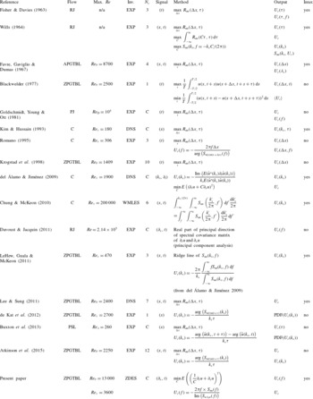
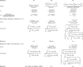
Inputs and outputs in the assessment of the convection velocity of streamwise velocity fluctuations in shear flows are displayed in table 1, covering some of the most striking studies in the literature, both experimental and numerical, with a special emphasis on boundary layers. Only the streamwise length scale is considered here, even though the dependence on the spanwise length scale is sometimes addressed, for example by Kim & Hussain (Reference Kim and Hussain1993) and del Álamo & Jiménez (Reference del Álamo and Jiménez2009). The streamwise velocity fluctuation
 $u(x,t)=U(x,t)-\langle U(x,t)\rangle$
is defined from the Reynolds average
 $\langle \cdot \rangle$
, where the dependence on
 $y$
and
 $z$
is omitted. If the fluctuation is exactly convected at the convection velocity
 $U_{c}$
, the following equation holds:
 $$\begin{eqnarray}\partial _{t}u+U_{c}\partial _{x}u=0,\end{eqnarray}$$
where
 $U_{c}>0$
corresponds to a convection towards
 $x>0$
.
Assessment of the convection velocity
 $U_{c}$
of the streamwise velocity fluctuations in shear flows. Flow: ZPGTBL, zero pressure gradient turbulent boundary layer; APGTBL, adverse pressure gradient turbulent boundary layer; C, channel; RJ, round jet; PJ, plane jet; PSL, plane shear layer. Inv. (investigation): EXP, experiment; DNS, direct numerical simulation; LES, large eddy simulation; WMLES, wall-modelled large eddy simulation; ZDES, zonal detached eddy simulation.
 $N_{y}$
: number of stations across the shear profile where
 $U_{c}$
is provided; C, whole shear profile covered with a fine discretization. Signal:
 $t$
, time signal available;
 $x$
, spatial signal;
 $\partial _{t}$
, time derivative of the signal available;
 $\partial _{x}$
, spatial derivative available;
 $f$
, time Fourier modes available;
 $k_{x}$
, streamwise Fourier modes available. Output:
 $U_{c}$
, global convection velocity;
 $U_{c}(\,f)$
, frequency-dependent convection velocity;
 $U_{c}(k_{x})$
, wavenumber-dependent convection velocity;
 $\text{PDF}(U_{c})$
, probability density function of
 $U_{c},S_{uu}(k_{x},U_{c})$
time–space power spectral density (PSD) expressed as a function of
 $k_{x}$
and
 $U_{c}$
. Inter. (interpretation): available interpretation of the value of
 $U_{c}$
even when Taylor’s hypothesis is not strictly valid.

From table 1, it appears that even though many studies have been devoted to the topic, including studies of boundary layers, there is no available dataset, to the authors’ knowledge, of the scale-dependent convection velocity of streamwise velocity fluctuations through the whole profile (rather than at a limited number of wall distances) of a zero-pressure-gradient boundary layer at a Reynolds number as high as that of the present study (
 $\mathit{Re}_{{\it\theta}}=13\,000$
). One of the reasons is the cost of the numerical simulation of developing boundary layers. To the authors’ knowledge, the current highest Reynolds number ranges achieved, based on the momentum thickness
 ${\it\theta}$
, are
 $\mathit{Re}_{{\it\theta}}=13\,320{-}15\,489$
(a relatively short Reynolds number range) for the direct numerical simulation of a compressible
 $M_{\infty }=2$
boundary layer by Pirozzoli & Bernardini (Reference Pirozzoli and Bernardini2013),
 $\mathit{Re}_{{\it\theta}}=2780{-}6650$
for an incompressible boundary layer DNS (direct numerical simulation) by Sillero et al. (Reference Sillero, Jiménez, Moser and Malaya2011),
 $\mathit{Re}_{{\it\theta}}=180{-}8300$
for a very well-resolved incompressible WRLES (wall-resolved large eddy simulation) by Eitel-Amor, Örlü & Schlatter (Reference Eitel-Amor, Örlü and Schlatter2014), and
 $\mathit{Re}_{{\it\theta}}=3060{-}13\,650$
for a WRLES by Deck et al. (Reference Deck, Renard, Laraufie and Weiss2014b
) at such a low Mach number that it may be considered incompressible. The latter simulation is used in the present study. The choice of a method to assess the convection velocity is discussed in the next section.
1.3. Need for a new spectral method to assess the convection velocity in spatially developing flows
In the following, the existing methods to investigate the scale-dependent convection velocity in spatially developing flows such as boundary layers are discussed, showing the need for a new method.
One class of methods relies on the maximization of the two-point two-time correlation of the streamwise velocity fluctuations (thoroughly discussed by Fisher & Davies Reference Fisher and Davies1963; Wills Reference Wills1964; Favre et al. Reference Favre, Gaviglio and Dumas1967). The result indirectly depends on the streamwise length scale of the fluctuation through the choice of the spatial or temporal separation before maximizing the correlation, since only the structures that have the longest life time (i.e. the largest ones) are taken into account when a large separation is retained. A direct assessment of the scale dependence is, however, greatly preferable. This may be obtained by band-pass filtering the signals (see e.g. Fisher & Davies Reference Fisher and Davies1963; Wills Reference Wills1964; Favre et al. Reference Favre, Gaviglio and Dumas1967; Goldschmidt et al. Reference Goldschmidt, Young and Ott1981; Kim & Hussain Reference Kim and Hussain1993). However, the phase of the signals must be rigorously preserved by the filter and aliasing should also be avoided (Goldschmidt et al. Reference Goldschmidt, Young and Ott1981). To circumvent these difficulties, an intrinsically spectral method is preferred.
In a flow that is statistically homogeneous along
 $x$
, stationary in time and when highly resolved data are available, a spectral convection velocity can be assessed from the frequency–wavenumber spectrum. Considering the space–time Fourier transform
 $\hat{u} (k_{x}/(2{\rm\pi}),f)$
of
 $u(x,t)$
,
 $$\begin{eqnarray}\displaystyle & \displaystyle \hat{u} \left(\frac{k_{x}}{2{\rm\pi}},f\right)=\int _{-\infty }^{\infty }\int _{-\infty }^{\infty }u(x,t)\exp (-\text{i}(2{\rm\pi}ft+k_{x}x))\,\text{d}t\,\text{d}x, & \displaystyle\end{eqnarray}$$
 $$\begin{eqnarray}\displaystyle & \displaystyle u(x,t)=\int _{-\infty }^{\infty }\int _{-\infty }^{\infty }\hat{u} \left(\frac{k_{x}}{2{\rm\pi}},f\right)\exp (\text{i}(2{\rm\pi}ft+k_{x}x))\,\text{d}f\frac{\text{d}k_{x}}{2{\rm\pi}}, & \displaystyle\end{eqnarray}$$
 $$\begin{eqnarray}2{\rm\pi}f=-U_{c}\,k_{x}.\end{eqnarray}$$
The convection velocity is assessed from frequency–wavenumber spectra in Wills (Reference Wills1964), Choi & Moin (Reference Choi and Moin1990), del Álamo & Jiménez (Reference del Álamo and Jiménez2009), Chung & McKeon (Reference Chung and McKeon2010) and LeHew et al. (Reference LeHew, Guala and McKeon2011), among others. Even though these methods inherently include scale dependence, they may not be retained here, because the spatial growth of the boundary layer is an obstacle to the computation of a streamwise spectrum. Reconstructing the latter without corrections for the spatial growth is precisely one of the motivations for the convection velocity estimation. Methods relying on frequency–wavenumber spectra are also limited by the required data storage in both time and space, especially at high Reynolds numbers. This motivates methods based on spectral data along only one direction (time or space). In the literature, such methods are often applied to the dual case when streamwise signals are available at a very limited number of points in time (e.g. in non-time-resolved PIV experiments). Because of the spatial growth of the boundary layer, we presently focus on the case of time signals available at a very limited number of streamwise points in the vicinity of the Reynolds number station considered.
One classical method relies on the phase of the signals; see Romano (Reference Romano1995) in the present case, de Kat et al. (Reference de Kat, Gan, Dawson and Ganapathisubramani2012) and Atkinson et al. (Reference Atkinson, Buchmann and Soria2015) in the dual case of streamwise signals at two points in time. The phase
 ${\it\Phi}_{u}(x,f)$
is defined modulo
 $2{\rm\pi}$
(for continuity) from the Fourier transform
 $\hat{u} (x,f)$
of the time signals:
 $$\begin{eqnarray}\displaystyle & \displaystyle \hat{u} (x,f)=\int _{-\infty }^{\infty }u(x,t)\exp (-\text{i}2{\rm\pi}ft)\,\text{d}t\Leftrightarrow u(x,t)=\int _{-\infty }^{\infty }\hat{u} (x,f)\exp (\text{i}2{\rm\pi}ft)\,\text{d}f, & \displaystyle\end{eqnarray}$$
 $$\begin{eqnarray}\displaystyle & \displaystyle u(x,t)=\int _{-\infty }^{\infty }|\hat{u} (x,f)|\exp (\text{i}({\it\Phi}_{u}(x,f)+2{\rm\pi}ft))\,\text{d}f. & \displaystyle\end{eqnarray}$$
 $2{\rm\pi}f=-U_{c}(\,f)\,k_{x}$
holds rigorously, non-zero-energy Fourier modes
 $(k_{x},f)$
verify
 $k_{x}=k_{x}(\,f)$
. This implies that all fluctuations are rigorously advected at the velocity
 $U_{c}(\,f)$
with no variation from one event to the other. Comparing (1.3) with (1.6) then leads to
 $$\begin{eqnarray}{\it\Phi}_{u}(x,f)=k_{x}(\,f)x+{\it\Phi}_{0}(\,f)=-\frac{2{\rm\pi}f}{U_{c}(\,f)}x+{\it\Phi}_{0}(\,f),\end{eqnarray}$$
and for signals at two points separated in the streamwise direction by
 ${\rm\Delta}x$
,
 $$\begin{eqnarray}U_{c}(\,f)=-\frac{2{\rm\pi}f{\rm\Delta}x}{{\it\Phi}_{u}(x+{\rm\Delta}x,f)-{\it\Phi}_{u}(x,f)}.\end{eqnarray}$$
However, the result fluctuates between independent realizations of the flow (see its probability density function in de Kat et al. Reference de Kat, Gan, Dawson and Ganapathisubramani2012 together with the average value). Averaged results are alternatively provided by the cross-PSD of the time signals:
 $$\begin{eqnarray}S_{u(x)u(x+{\rm\Delta}x)}(\,f)=\int _{-\infty }^{\infty }R_{u(x)u(x+{\rm\Delta}x)}({\it\tau})\exp (-\text{i}2{\rm\pi}f{\it\tau})\,\text{d}{\it\tau},\end{eqnarray}$$
where
 $R_{u(x)u(x+{\rm\Delta}x)}({\it\tau})=E(u(x,t)u(x+{\rm\Delta}x,t+{\it\tau}))$
. If the flow is homogeneous along
 $x$
and if
 $U_{c}(\,f)$
does not fluctuate, so that the phase difference
 ${\it\Phi}_{u}(x+{\rm\Delta}x,f)-{\it\Phi}_{u}(x,f)={\rm\Delta}{\it\Phi}_{u}({\rm\Delta}x,f)$
is always the same, then
 $$\begin{eqnarray}S_{u(x)u(x+{\rm\Delta}x)}(\,f)=S_{uu}(\,f)\exp (\text{i}{\rm\Delta}{\it\Phi}_{u}({\rm\Delta}x,f))\end{eqnarray}$$
and (1.8) becomes
 $$\begin{eqnarray}U_{c}(\,f)=-\frac{2{\rm\pi}f{\rm\Delta}x}{\arg (S_{u(x)u(x+{\rm\Delta}x)}(\,f))}.\end{eqnarray}$$
The assumption that the convection velocity does not fluctuate is not verified in a turbulent flow, so that (1.11) and the average result of (1.8) do not necessarily coincide. There seems to be no physical interpretation of the two resulting ‘average’ values of the convection velocity. Furthermore, both (1.8) and (1.11) depend on the value of
 ${\rm\Delta}x$
(see Romano Reference Romano1995). The larger
 ${\rm\Delta}x$
, the longer time the perturbations evolve in other ways than pure convection. Further, too small a value of
 ${\rm\Delta}x$
may alter the assessment of the argument of
 $S_{u(x)u(x+{\rm\Delta}x)}(\,f)$
, which becomes small compared with noise.
Another possibility is the method by del Álamo & Jiménez (Reference del Álamo and Jiménez2009) using in the dual case the streamwise spectra and their time derivative at one point in time. In the present case, briefly described in del Álamo & Jiménez (Reference del Álamo and Jiménez2009), time spectra and their local streamwise derivative are needed, as detailed here. Coming back to the decomposition of the signal in time Fourier modes (1.6), the local convection velocity
 $U_{c}(x;f)$
of the Fourier mode of frequency
 $f$
is defined as its phase velocity, providing local stationarity of the phase:
 $$\begin{eqnarray}\displaystyle & \displaystyle \left(\frac{\partial ({\it\Phi}_{u}(x(t),f)+2{\rm\pi}ft)}{\partial t}\right)_{\text{d}x/\text{d}t=U_{c}(x;f)}=0\;\left(\Leftrightarrow U_{c}(x;f)\frac{\partial {\it\Phi}_{u}(x,f)}{\partial x}+2{\rm\pi}f=0\right),\quad & \displaystyle\end{eqnarray}$$
 $$\begin{eqnarray}\displaystyle & \displaystyle U_{c}(x;f)=-\frac{2{\rm\pi}f}{\displaystyle \frac{\partial {\it\Phi}_{u}(x,f)}{\partial x}}. & \displaystyle\end{eqnarray}$$
 $x$
(1.7). This is not the case when Taylor’s hypothesis is not strictly valid, whereas (1.13) still provides the exact local phase velocity. The latter equation may be modified as follows:
 $$\begin{eqnarray}U_{c}(x;f)=-\frac{2{\rm\pi}f\hat{u} (x,f)\hat{u} (x,f)^{\ast }}{\displaystyle \hat{u} (x,f)\hat{u} (x,f)^{\ast }\frac{\partial {\it\Phi}_{u}(x,f)}{\partial x}},\end{eqnarray}$$
where
 $^{\ast }$
denotes the complex conjugate. The time Fourier transform
 $\partial _{x}\hat{u} (x,f)$
of
 $\partial _{x}u(x,t)$
is obtained by deriving
 $\hat{u} (x,f)=|\hat{u} (x,f)|\exp (\text{i}{\it\Phi}_{u}(x,f))$
(1.6) with respect to
 $x$
,
 $$\begin{eqnarray}\partial _{x}\hat{u} (x,f)=(\partial _{x}\left|\hat{u} (x,f)\right|+\left|\hat{u} (x,f)\right|\text{i}\partial _{x}{\it\Phi}_{u}(x,f))\exp (\text{i}{\it\Phi}_{u}(x,f))\end{eqnarray}$$
from which one finds that the following equation (equation (2.17) in del Álamo & Jiménez Reference del Álamo and Jiménez2009), is equivalent to (1.14):
 $$\begin{eqnarray}U_{c}(x;f)=-\frac{2{\rm\pi}f\hat{u} (x,f)^{\ast }\hat{u} (x,f)}{\text{Im}(\hat{u} (x,f)^{\ast }\partial _{x}\hat{u} (x,f))},\end{eqnarray}$$
where
 $\text{Im}(\cdot )$
denotes the imaginary part. In (1.16), even when a pure convection process at a unique convection velocity and frequency is involved, the derivative is applied to a nonlinear function of
 $x$
, contrary to (1.13), so that care must be taken in the evaluation of the streamwise derivative, for which a first-order approximation is not sufficient. However, the accuracy of the discrete evaluation of (1.16) can be enhanced not only by reducing the streamwise separation
 ${\rm\Delta}x$
between the signals, but also by adding more points to the stencil used (i.e. more signal locations). This transforms the problem in choosing the value of
 ${\rm\Delta}x$
for (1.8) into a better-known optimization of derivative evaluation in (1.16), using for instance high-order finite difference schemes with explicit evaluation of the numerical error.
However, averaging (1.16) over several independent realizations is not trivial, because
 $U_{c}(x;f)$
is a ratio of two quantities, and its average is not necessarily equal to the ratio of these averaged quantities. Moreover, the present study relies on a numerical simulation with a finite time length and no periodicity, so that the time Fourier modes involved in (1.16) may not be directly obtained (in the dual case of del Álamo & Jiménez Reference del Álamo and Jiménez2009, the spatial Fourier modes came from the spectral DNS solver). Power spectral densities may be estimated instead, but relating them to the Fourier modes in (1.16) once again involves averaging. This seems not totally rigorous because of the ratio of averages differing from the averaged ratio, except once again in the unphysical case of a non-fluctuating convection velocity (indeed, if the ratio
 $k=A/B$
of two quantities
 $A$
and
 $B$
does not fluctuate, then
 $A$
and
 $B$
are linearly dependent (
 $A=kB$
), so that
 $E(A/B)=k=E(A)/E(B)$
).
In addition to the wavenumber-dependent convection velocity defined as the phase velocity (similarly to (1.16)), del Álamo & Jiménez (Reference del Álamo and Jiménez2009) also introduce a global convection velocity that represents the convection at all scales, based on the minimization of the squared residual of the convection equation. Only the case of streamwise spectra and their time derivative is treated by del Álamo & Jiménez (Reference del Álamo and Jiménez2009), but there is no obstacle to treating the present dual case in a similar way, even though it is not found in the literature. The optimization inherently measures the validity of Taylor’s hypothesis through a correlation coefficient. If the signal is made of a single Fourier mode of wavenumber
 $k_{x}$
, then the global convection velocity reduces to the wavenumber-dependent phase velocity
 $U_{c}(k_{x})$
(dual to (1.16)). Del Álamo & Jiménez (Reference del Álamo and Jiménez2009) finally express the global velocity as a weighted average of the wavenumber-dependent phase velocity, so that the convection velocity corresponding to any chosen wavenumber band may be assessed.
There exists a variant of the method of del Álamo & Jiménez (Reference del Álamo and Jiménez2009), by Davoust & Jacquin (Reference Davoust and Jacquin2011), which was applied in an experimental round jet where time signals and their local spatial derivative are available (like the present numerical simulation case, and dual to del Álamo & Jiménez Reference del Álamo and Jiménez2009). The frequency-dependent convection velocity is determined from the real part of the principal direction of the spectral covariance matrix of
 $\partial _{t}u$
and
 $\partial _{x}u$
. The results coincide with the method of del Álamo & Jiménez (Reference del Álamo and Jiménez2009) when the validity of Taylor’s hypothesis is good, but they differ when processes other than pure convection are involved. Even though it seems to be more robust in the presence of noisy experimental data, this principal components analysis does not shed much light on the physical meaning of the result when Taylor’s hypothesis validity is not very good, and similarly for the method of the phase of the cross-spectrum.
For the present study, the method of del Álamo & Jiménez (Reference del Álamo and Jiménez2009) is consequently preferred to other methods. Indeed, only data at the considered
 $x$
location is involved, the streamwise evolution being described by the local derivative. Locality is crucial in a spatially developing flow. Moreover, the validity of Taylor’s hypothesis is intrinsically assessed, and there is potential for interpretation of the result even when the hypothesis is not strictly valid. Furthermore, it circumvents the problematic choice of the streamwise separation
 ${\rm\Delta}x$
inherent to the cross-spectrum phase method.
However, several difficulties arise in applying the method of del Álamo & Jiménez (Reference del Álamo and Jiménez2009) to the present study. First, del Álamo & Jiménez (Reference del Álamo and Jiménez2009) rely on spatial Fourier modes that are readily available from the spectral DNS solver. Here only estimated PSDs from signals of finite length are available. Use of these estimates was briefly suggested in del Álamo & Jiménez (Reference del Álamo and Jiménez2009), but is not totally straightforward and requires some mathematical care, as well as averaging over independent flow realizations. Further, del Álamo & Jiménez (Reference del Álamo and Jiménez2009) only suggested the expression for the phase velocity in the dual case, which has to be considered because the present (boundary layer) flow is spatially developing, contrary to their (channel) flow. Consequently, deriving the global convection velocity, its relation to the phase velocity, and the correlation coefficient that assesses the validity of Taylor’s hypothesis is required for the present study. Finally, the global convection velocity of del Álamo & Jiménez (Reference del Álamo and Jiménez2009) has a somewhat mathematical interpretation based on least-squares optimization. An interpretation based on the flow physics is lacking in the literature. This motivates the derivation, interpretation and assessment of a new spectral method based on del Álamo & Jiménez (Reference del Álamo and Jiménez2009) for the present study, whose organization is indicated in the next section.
1.4. Outline of the paper
To address the needs of the present study, a new spectral method is first derived in § 2 and illustrated in § 3 in a test case representative of high Reynolds number spatially developing turbulent flows. Next the reconstruction of the streamwise spectrum from the temporal spectrum using the convection velocity is demonstrated (§ 4), a global convection velocity is defined and compared with more classical global velocities (§ 5), and physical interpretations of the global velocity are presented (§ 6). Finally, § 7 discusses the group velocity.
2. A new method for the spectral assessment of the convection velocity in spatially developing flows
The new method to assess the scale-dependent convection velocity derived in the present section is inspired by del Álamo & Jiménez (Reference del Álamo and Jiménez2009). They made use of streamwise Fourier modes and their time derivative in a streamwise homogeneous flow, and suggested that the dual problem could be addressed, i.e. the roles of time and space could be swapped. The derivation of a dual method using time signals and their local spatial derivative, which is necessary to cope with the streamwise heterogeneity, has not been detailed in the literature before. Besides, it is shown how estimates of the PSD of the time signals may be used instead of explicit Fourier modes which are not available from unsteady numerical simulations.
2.1. Global definition of the convection velocity
As mentioned in the Introduction, since Taylor’s hypothesis is not rigorously valid in wall-bounded turbulence, the convection velocity
 $C$
does not necessarily coincide with the mean velocity and should be defined as the value of
 $C$
for which the following convection equation best describes the fluctuations:
 $$\begin{eqnarray}\frac{1}{C}\partial _{t}u+\partial _{x}u=0.\end{eqnarray}$$
For the optimal value of
 $C$
, the square of the residual
 $(1/C)\partial _{t}u+\partial _{x}u$
of the convection equation is not expected to rigorously vanish, but it is as close to zero as possible. The present global convection velocity
 $C_{u}$
, which accounts for all scales, is the value of
 $C$
that provides the minimum value of
 $\mathscr{D}(C)$
, where
 $$\begin{eqnarray}\mathscr{D}(C)=\frac{\displaystyle E\left(\left(\frac{1}{C}\partial _{t}u+\partial _{x}u\right)^{2}\right)}{E((\partial _{x}u)^{2})}.\end{eqnarray}$$
It should be noted that in their case, del Álamo & Jiménez (Reference del Álamo and Jiménez2009) minimized the dual quantity
 $(E((\partial _{t}u+C\partial _{x}u)^{2})/E((\partial _{t}u)^{2}))$
. The roles of the streamwise and temporal derivatives are swapped consistently with the derivation of a dual method suited to spatially developing flows. Crucially, the expectation of the squared residual of the convection equation is normalized by a quantity that does not depend on the convection velocity
 $C$
. Minimizing either
 $\mathscr{D}(C)$
or
 $E(((1/C)\partial _{t}u+\partial _{x}u)^{2})$
over
 $C$
is equivalent, and leads to the following condition for
 $C_{u}$
:
 $$\begin{eqnarray}\frac{\partial \mathscr{D}}{\partial C}(C_{u})=0\Rightarrow C_{u}=-\frac{E((\partial _{t}u)^{2})}{E(\partial _{t}u\,\partial _{x}u)}.\end{eqnarray}$$
This differs from the dual global convection velocity defined in equation (2.4) of del Álamo & Jiménez (Reference del Álamo and Jiménez2009) as
 $-(E(\partial _{t}u\partial _{x}u)/E((\partial _{x}u)^{2}))$
. A discussion on how a different choice of the quantity to be minimized leads to other definitions of the convection velocity may be found in appendix A. It should be noted that (2.3) involves only local signals at the streamwise location
 $x$
, a strong advantage in a spatially developing flow such as the boundary layer since one of the motivations for assessing the convection velocity is to recover a fictitious spatial spectrum from time signals at the chosen Reynolds number station. Besides the least-squares definition of the global convection velocity, an interpretation based on turbulence physics in a moving frame of reference is given in § 6. Moreover, it will be demonstrated in § 5.2 that the present convection velocity is equivalent to a correlation-based definition commonly used in experiments.
The smaller
 $\mathscr{D}(C_{u})$
, the higher the level of validity of Taylor’s hypothesis. We define a suitable correlation coefficient by
 $$\begin{eqnarray}1-{\it\gamma}_{u}^{2}=\mathscr{D}(C_{u}),\quad {\it\gamma}_{u}\geqslant 0,\quad \text{so that }{\it\gamma}_{u}=\frac{|E(\partial _{t}u\,\partial _{x}u)|}{\sqrt{E((\partial _{t}u)^{2})E((\partial _{x}u)^{2})}}.\end{eqnarray}$$
Here
 ${\it\gamma}_{u}$
varies between 1 (perfect convection process, vanishing
 $\mathscr{D}(C_{u})$
) and 0. Remarkably it coincides with the dual case given by equation (2.5) of del Álamo & Jiménez (Reference del Álamo and Jiménez2009), unlike the convection velocity
 $C_{u}$
. The closer to frozen are the turbulent fluctuations, the more correlated are their time and space derivatives, because the residual of (2.1) is smaller.
The mathematical expectations involved in the convection velocity
 $C_{u}$
(2.3) and in the associated correlation coefficient
 ${\it\gamma}_{u}$
(2.4) are assessed using the PSD of the time signals, which may be estimated using Welch’s method because the signals are statistically stationary. Recall that the cross-power spectral density
 $S_{ab}(\,f)$
of signals
 $a(t)$
and
 $b(t)$
is defined by
 $$\begin{eqnarray}R_{ab}({\it\tau})=E(a(t)b(t+{\it\tau})),\end{eqnarray}$$
 $$\begin{eqnarray}S_{ab}(\,f)=\int _{-\infty }^{\infty }R_{ab}({\it\tau})\exp (-\text{i}2{\rm\pi}f{\it\tau})\,\text{d}{\it\tau},\quad R_{ab}({\it\tau})=\int _{-\infty }^{\infty }S_{ab}(\,f)\exp (\text{i}2{\rm\pi}f{\it\tau})\,\text{d}f.\end{eqnarray}$$
From (2.3), (2.5) and (2.6), the equation for the convection velocity becomes
 $$\begin{eqnarray}C_{u}=-\frac{\displaystyle \int _{-\infty }^{\infty }S_{\partial _{t}u\partial _{t}u}(\,f)\,\text{d}f}{\displaystyle \int _{-\infty }^{\infty }S_{\partial _{t}u\,\partial _{x}u}(\,f)\,\text{d}f}.\end{eqnarray}$$
There is no need to estimate the time derivative of the signal, thanks to the two following properties, for statistically stationary time signals
 $a(t)$
and
 $b(t)$
:
 $$\begin{eqnarray}S_{a\,\partial _{t}b}(\,f)=2\text{i}{\rm\pi}fS_{ab}(\,f)\quad \text{and}\quad S_{\partial _{t}a\;b}(\,f)=-2\text{i}{\rm\pi}fS_{ab}(\,f),\end{eqnarray}$$
where the assumption of statistical stationarity is necessary for the latter equation (see appendix B). Equation (2.7) then becomes
 $$\begin{eqnarray}C_{u}=-\frac{\displaystyle \int _{-\infty }^{\infty }(2{\rm\pi}f)^{2}S_{uu}(\,f)\,\text{d}f}{\displaystyle \int _{-\infty }^{\infty }-2\text{i}{\rm\pi}fS_{u\,\partial _{x}u}(\,f)\,\text{d}f}.\end{eqnarray}$$
Since
 $u(t)$
is stationary,
 $S_{uu}(\,f)$
is real-valued and symmetrical (
 $S_{uu}(-f)=S_{uu}(\,f)$
). Moreover,
 $S_{u\,\partial _{x}u}(-f)=S_{u\,\partial _{x}u}(\,f)^{\ast }$
(Hermitian symmetry), so (2.7) finally becomes
 $$\begin{eqnarray}C_{u}=-\frac{\displaystyle \int _{0}^{\infty }(2{\rm\pi}f)^{2}S_{uu}(\,f)\,\text{d}f}{\displaystyle \int _{0}^{\infty }2{\rm\pi}f\,\text{Im}(S_{u\,\partial _{x}u}(\,f))\,\text{d}f}.\end{eqnarray}$$
In the same way, (2.4) may be rewritten as
 $$\begin{eqnarray}\displaystyle & \displaystyle {\it\gamma}_{u}=\frac{\displaystyle \left|\int _{-\infty }^{\infty }-2\text{i}{\rm\pi}fS_{u\,\partial _{x}u}(\,f)\,\text{d}f\right|}{\displaystyle \sqrt{\int _{-\infty }^{\infty }(2{\rm\pi}f)^{2}S_{uu}(\,f)\,\text{d}f}\sqrt{\int _{-\infty }^{\infty }S_{\partial _{x}u\,\partial _{x}u}(\,f)\,\text{d}f}}, & \displaystyle\end{eqnarray}$$
 $$\begin{eqnarray}\displaystyle & \displaystyle {\it\gamma}_{u}=\frac{\displaystyle \left|\int _{0}^{\infty }2{\rm\pi}f\,\text{Im}(S_{u\,\partial _{x}u}(\,f))\,\text{d}f\right|}{\displaystyle \sqrt{\int _{0}^{\infty }(2{\rm\pi}f)^{2}S_{uu}(\,f)\,\text{d}f}\sqrt{\int _{0}^{\infty }S_{\partial _{x}u\,\partial _{x}u}(\,f)\,\text{d}f}}. & \displaystyle\end{eqnarray}$$
 $u(t)$
and of its local spatial derivative
 $\partial _{x}u(t)$
. Since integrals over frequency are involved, the frequency-dependent convection velocity and correlation coefficient are derived in a very natural way in the next section.
2.2. Frequency-dependent convection velocity
A frequency-dependent convection velocity may be identified with the phase velocity of a single Fourier mode, as illustrated in the Introduction (1.16). While this is done by del Álamo & Jiménez (Reference del Álamo and Jiménez2009), where discrete Fourier modes were readily available from the spectral code, transposition to the present dual case is not obvious. Indeed, the time signals from numerical simulations have a finite length, so that the PSD estimation represents the average contribution of a frequency band of finite width to the energy of the signal. On the contrary, the physical problem is defined over an infinite time length, so that there exists an infinity of time Fourier modes
 $(\,f)$
continuously distributed over the frequency range, each mode having zero probability of being encountered because of its zero frequency support width. One singular Fourier mode
 $(\,f)$
of finite amplitude, whose phase velocity is given by (1.16), consequently has zero average contribution to the signal energy because it has zero probability of existing. Moreover, averaging (1.16) is problematic, as emphasized in the Introduction. Because of the nature of the time signals available from numerical simulations, the present frequency-dependent convection velocity is derived by restricting the global convection velocity (2.10) to a frequency band in the limit of a vanishing width. The resulting formula depends on the power spectral density instead of the amplitude of a singular Fourier mode as in del Álamo & Jiménez (Reference del Álamo and Jiménez2009) and (1.16).
As mentioned in the Introduction, the velocity signals may be filtered before using (2.3) to obtain the convection velocity of the pass-filtered scales. However, filtering may result in aliasing and phase alteration. Instead of filtering, it is preferable to take advantage of the frequency decomposition already displayed by (2.10). The time Fourier transform and the streamwise derivation commute,
 $\widehat{\partial _{x}u}(\,f)=\partial _{x}\hat{u} (\,f)$
, because
 $x$
and
 $t$
are independent coordinates. Consequently, both signals
 $u(t)$
and
 $\partial _{x}u(t)$
involved in (2.10) are affected in the same way by a frequency filtering, and the upper and lower integrals in (2.10) may be restricted to the same narrow frequency band. The convection velocity
 $C_{u}(f_{0},{\it\epsilon})$
associated with the energy contained in a frequency band
 $[\,f_{0}-{\it\epsilon},f_{0}+{\it\epsilon}]$
becomes
 $$\begin{eqnarray}C_{u}(f_{0},{\it\epsilon})=-\frac{\displaystyle \int _{f_{0}-{\it\epsilon}}^{f_{0}+{\it\epsilon}}(2{\rm\pi}f)^{2}S_{uu}(\,f)\,\text{d}f}{\displaystyle \int _{f_{0}-{\it\epsilon}}^{f_{0}+{\it\epsilon}}2{\rm\pi}f\,\text{Im}(S_{u\,\partial _{x}u}(\,f))\,\text{d}f}.\end{eqnarray}$$
The formula for the frequency-dependent convection velocity
 $U_{c}(f_{0})=\lim _{{\it\epsilon}\rightarrow 0}C_{u}(f_{0},{\it\epsilon})$
is obtained for a vanishing bandwidth
 $2{\it\epsilon}\rightarrow 0$
. As soon as the PSDs are continuous, it reads
 $$\begin{eqnarray}U_{c}(\,f)=-\frac{2{\rm\pi}fS_{uu}(\,f)}{\text{Im}(S_{u\,\partial _{x}u}(\,f))}.\end{eqnarray}$$
The same derivation from (2.12) leads to the associated frequency-dependent correlation coefficient
 $$\begin{eqnarray}{\it\gamma}_{u}(\,f)=\frac{|\text{Im}(S_{u\,\partial _{x}u}(\,f))|}{\sqrt{S_{uu}(\,f)}\sqrt{S_{\partial _{x}u\,\partial _{x}u}(\,f)}}.\end{eqnarray}$$
The resulting frequency-dependent convection velocity (2.14) is very similar to the phase velocity of a single Fourier mode (1.16)
 $U_{c}(x;f)=-(2{\rm\pi}f\hat{u} (x,f)^{\ast }\hat{u} (x,f)/\text{Im}(\hat{u} (x,f)^{\ast }\partial _{x}\hat{u} (x,f)))$
, but it is suited to averaged power spectral densities. The issue of averaging (1.16) over several realizations, which is tackled by del Álamo & Jiménez (Reference del Álamo and Jiménez2009) by considering the ratio of the expectations
 $-(2{\rm\pi}fE(\hat{u} (x,f)^{\ast }\hat{u} (x,f))/\text{Im}(E(\hat{u} (x,f)^{\ast }\partial _{x}\hat{u} (x,f))))$
(not necessarily matching the expectation of the ratio), is naturally addressed here if the PSD is seen as a kind of averaging. In the simple case of a monochromatic perturbation at a constant convection velocity, (2.14) may be interpreted as the phase velocity. Otherwise, the interpretation relies on the least-squares optimization and infinitely narrow frequency-band restriction presented above. Regarding the correlation coefficient (2.15), no interpretation similar to the phase velocity seems possible for a single Fourier mode (none is given by del Álamo & Jiménez Reference del Álamo and Jiménez2009), so that its interpretation always relies on the least-squares derivation and frequency restriction.
The evaluation of (2.14) and (2.15) requires accurate computation of the local streamwise derivative of the time signal,
 $\partial _{x}u(t)$
(see the Introduction). Compared with the phase of the cross-spectrum method, which may be seen as a first-order approximation relying on only two streamwise stations, the streamwise derivatives in (2.14) and (2.15) may be assessed with high-order centred finite difference schemes using more than two streamwise stations, for which the evaluation of the numerical error is straightforward. Data storage must consequently be chosen in order to procure satisfying accuracy in the wavenumber range of interest specific to the available database, as illustrated in the next section.
3. Method illustration in a zero-pressure-gradient boundary layer at
 $\mathit{Re}_{{\it\theta}}=13\,000$

The method derived in the previous section is meant for spatially developing turbulent flows, thanks to its local streamwise formulation, and for high Reynolds numbers, where it significantly reduces data storage compared with methods based on frequency–wavenumber spectra. A natural test case is the spatially developing boundary layer at high Reynolds numbers. Superstructures cannot be easily observed at Reynolds numbers smaller than
 $\mathit{Re}_{{\it\theta}}=10^{4}$
because of the insufficient scale separation from other coherent motions. However, as recalled in the Introduction, no subsonic direct numerical simulation over a long streamwise numerical domain favourable to the full development of the largest coherent motions has been published for
 $\mathit{Re}_{{\it\theta}}>10^{4}$
, because of the computational cost involved. As a result, the new method is assessed on the resolved fluctuations from a wall-resolved large eddy simulation (WRLES). This not only indicates what may be expected from a future DNS dataset, especially thanks to the high resolution in the outer layer, and enables comparison with classical streamwise spectrum reconstruction methods, but also illustrates the relevance of convection velocity information to investigate the accuracy of turbulence models by determining whether or not resolved fluctuations are physically grounded, for example in the inner layer which is under-resolved compared with DNS. The numerical dataset used for the present illustration at
 $\mathit{Re}_{{\it\theta}}=13\,000$
has been thoroughly validated in Deck et al. (Reference Deck, Renard, Laraufie and Weiss2014b
) and is briefly presented in the following.
3.1. Turbulent boundary layer dataset used for the illustration
The compressible Navier–Stokes equations are solved on multiblock-structured grids using the FLU3M code developed by ONERA. Implicit time integration is carried out by the second-order backward scheme of Gear. The convective fluxes are discretized by a modified low-dissipative
 $\text{AUSM}+(\text{P})$
scheme (Mary & Sagaut Reference Mary and Sagaut2002). The solver accuracy has been assessed for direct numerical simulation and large eddy simulation by comparison with experimental data including spectra in many studies involving various types of flows (see e.g. Larchevêque et al.
Reference Larchevêque, Sagaut, Lê and Comte2004; Dandois, Garnier & Sagaut Reference Dandois, Garnier and Sagaut2007; Deck & Thorigny Reference Deck and Thorigny2007; Simon et al.
Reference Simon, Deck, Guillen, Sagaut and Merlen2007; Weiss et al.
Reference Weiss, Deck, Robinet and Sagaut2009; Gand et al.
Reference Gand, Deck, Brunet and Sagaut2010; Weiss & Deck Reference Weiss and Deck2011). Wall-bounded turbulent flows have been addressed using the third mode of zonal detached eddy simulation (ZDES) as a wall-modelled large eddy simulation (WMLES) in Deck et al. (Reference Deck, Weiss, Pamiès and Garnier2011), Laraufie, Deck & Sagaut (Reference Laraufie, Deck and Sagaut2011), Laraufie, Deck & Sagaut (Reference Laraufie, Deck, Sagaut, Fu, Haase, Peng and Schwamborn2012), Deck & Laraufie (Reference Deck and Laraufie2013), Laraufie & Deck (Reference Laraufie and Deck2013) and in Deck et al. (Reference Deck, Renard, Laraufie and Sagaut2014a
). The use of this technique to perform WRLES is demonstrated in Deck et al. (Reference Deck, Renard, Laraufie and Weiss2014b
) with the simulation used for the present study. Details of the formulation of the ZDES technique may be found in Deck (Reference Deck2012). The turbulent inflow is provided by the synthetic eddy method adapted from Jarrin et al. (Reference Jarrin, Benhamadouche, Laurence and Prosser2006) by Pamiès et al. (Reference Pamiès, Weiss, Garnier, Deck and Sagaut2009) and extended to ZDES by Deck et al. (Reference Deck, Weiss, Pamiès and Garnier2011).
A spatially developing smooth flat plate zero-pressure-gradient turbulent boundary layer has been simulated over a very large range of Reynolds numbers,
 $3060\leqslant \mathit{Re}_{{\it\theta}}\leqslant 13\,650~(1070\leqslant \mathit{Re}_{{\it\tau}}\leqslant 3800)$
, in Deck et al. (Reference Deck, Renard, Laraufie and Weiss2014b
). The low free-stream Mach number
 $M_{\infty }=0.21$
and the no-slip adiabatic wall condition imply that direct comparisons with incompressible simulations and very low Mach number experiments are possible. The WRLES mesh resolution is
 ${\rm\Delta}x^{+}=50$
and
 ${\rm\Delta}z^{+}=12$
in the streamwise and spanwise directions respectively, so that the inner site dynamics is not modelled, even though it is under-resolved compared with DNS. The first mesh cell is located within one wall unit from the wall. The outer layer is finely discretized so that the subgrid scales carry a negligible turbulent kinetic energy there (Deck et al.
Reference Deck, Renard, Laraufie and Weiss2014b
). 125 points are clustered in the boundary layer thickness
 ${\it\delta}_{13\,000}$
at
 $\mathit{Re}_{{\it\theta}}=13\,000$
. The computational domain is
 $342\,{\it\delta}_{0}$
long,
 $8.6\,{\it\delta}_{0}$
wide and
 $41\,{\it\delta}_{0}$
high, where
 ${\it\delta}_{0}$
is the initial boundary layer thickness, leading to a total number of grid points
 $N_{xyz}=806\times 10^{6}$
. The inner-scaled time step is very fine, around
 ${\rm\Delta}t^{+}=0.26$
, meeting the criterion by Choi & Moin (Reference Choi and Moin1994). Time signals are collected at the
 $\mathit{Re}_{{\it\theta}}=13\,000$
station over
 $1155\,{\it\delta}_{0}/U_{\infty }$
inertial times, where
 $U_{\infty }$
is the free-stream velocity. Nearly
 $2\times 10^{6}$
CPU hours have been spent on 936 Nehalem processors of the CINES superscalar computer Jade-SGI Altix Ice 8200. Three terabytes of data from selected volumes of the unsteady field have been stored, which is much less than would be needed to compute frequency–wavenumber spectra.
The numerical dataset has been thoroughly validated, including spectral data, in Deck et al. (Reference Deck, Renard, Laraufie and Weiss2014b
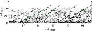
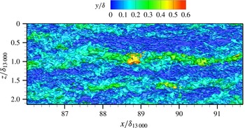
). Two visualizations relevant to the present study are presented in figures 1 and 2. This provides an insight not only into the shape of the largest resolved coherent motions near
 $\mathit{Re}_{{\it\theta}}=13\,000$
but also into physical space when interpreting spectral data.
Numerical schlieren (magnitude of density gradient in a streamwise/wall-normal plane) near the
 $\mathit{Re}_{{\it\theta}}=13\,000$
station.

 $u^{+}=20$
isosurface coloured by the wall distance near the
 $\mathit{Re}_{{\it\theta}}=13\,000$
station.

Figure 1 presents a numerical schlieren in a streamwise/wall-normal plane near the
 $\mathit{Re}_{{\it\theta}}=13\,000$
station, revealing the presence of inclined structures through the whole boundary layer thickness, which suggest packets of hairpins, consistent with the experimental findings leading to the hairpin packet paradigm of Adrian et al. (Reference Adrian, Meinhart and Tomkins2000). Some of these structures are indicated by dashed lines. The length of these packets is typically
 $1\,{\it\delta}$
to
 $3\,{\it\delta}$
, scaling with the local boundary layer thickness. Figure 2 presents, on the other hand, a horizontal plane projection of the isosurface of the instantaneous streamwise velocity
 $u^{+}=20$
, coloured by the wall distance. This reveals the presence of very long, meandering areas of low velocity (i.e. the given velocity level is reached much higher in the boundary layer, so that it appears in green to red instead of blue). This kind of coherent motion, which is more than
 $5\,{\it\delta}$
long, has been described in more detail in Deck et al. (Reference Deck, Renard, Laraufie and Weiss2014b
), suggesting that these are resolved superstructures. It should be noted that the superstructures seen in figure 2 are longer than the packets of hairpins identified in figure 1. The scale separation and its Reynolds number dependence are characterized in the next section by spectral analysis. The separation should be large enough for the scale-dependent convection velocity analysis to be relevant.
3.2. A brief spectral characterization of the resolved streamwise velocity fluctuations
The time PSD defined in (2.5) and (2.6) is estimated by Welch’s method (Welch Reference Welch1967) and further averaged in the spanwise direction. When both investigated signals coincide, the one-sided PSD
 $G_{aa}(\,f)\;(=2S_{aa}(\,f)$
for
 $f>0)$
of the statistically stationary time signal
 $a(t)$
is preferred, leading to
 $$\begin{eqnarray}\int _{0}^{\infty }G_{aa}(\,f)\,\text{d}f=E(a^{2})~\left(=\int _{0}^{\infty }G_{aa}({\it\omega})\,\text{d}{\it\omega}\right).\end{eqnarray}$$
In the following, the variable between brackets will implicitly denote the support of the PSD. For instance,
 $G_{aa}(\,f)$
and
 $G_{aa}({\it\omega})$
differ by a factor
 $2{\rm\pi}$
.
Here the streamwise PSD of the streamwise velocity fluctuations
 $G_{uu}(k_{x})$
is presented, and pre-multiplied so that the area below its semi-logarithmic plot is proportional to the variance:
 $$\begin{eqnarray}E(u^{2})=\int _{0}^{\infty }G_{uu}(k_{x})\,\text{d}k_{x}=\int _{-\infty }^{\infty }k_{x}G_{uu}(k_{x})\,\text{d}\ln (k_{x}).\end{eqnarray}$$
The streamwise PSD (depending on the streamwise wavenumber
 $k_{x}$
) is reconstructed from the estimated time PSD (depending on the frequency
 $f$
) using Taylor’s hypothesis with the local Reynolds-averaged streamwise velocity as the convection velocity (
 $U_{c}=\langle U\rangle (y)$
). This choice enables comparison with experimental spectra which are deduced from time signals in the same manner. The one-sided pre-multiplied streamwise PSD of streamwise velocity
 $k_{x}G_{uu}(k_{x})/u_{{\it\tau}}^{2}$
non-dimensionalized by the friction velocity at the station
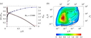
 $\mathit{Re}_{{\it\theta}}=13\,000~(\mathit{Re}_{{\it\tau}}=3600)$
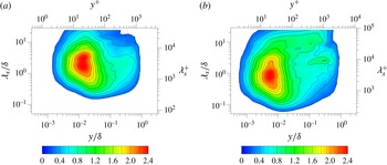
is plotted in figure 3 versus the wall distance and the streamwise wavelength together with experimental data at similar Reynolds numbers. Along with the streamwise mean velocity and turbulence intensity profiles, this reveals overall good agreement of the present simulation with the experiments, the outer layer being especially well resolved, as shown in more detail in Deck et al. (Reference Deck, Renard, Laraufie and Weiss2014b
). The outer energy site at large wavelengths (of the order of
 $6\,{\it\delta}$
) is well captured by the simulation. This is consistent with the visualization (figure 2) of the superstructures, to which this site corresponds (see Marusic, Mathis & Hutchins Reference Marusic, Mathis and Hutchins2010). Consistent with the WRLES modelling strategy, the inner layer is somewhat under-resolved.
Streamwise velocity profiles at
 $\mathit{Re}_{{\it\theta}}=13\,000~(\mathit{Re}_{{\it\tau}}=3600)$
. (a) Mean velocity (solid line) compared with experimental data by DeGraaff & Eaton (Reference DeGraaff and Eaton2000) (circles), and
 $u_{rms}^{+}$
(dash-dotted line) compared with the model by Marusic, Uddin & Perry (Reference Marusic, Uddin and Perry1997) and Marusic & Kunkel (Reference Marusic and Kunkel2003) (squares). (b) One-sided pre-multiplied streamwise PSD of streamwise velocity
 $k_{x}G_{uu}(k_{x})/u_{{\it\tau}}^{2}$
(dispersion relation
 $U_{c}=\langle U\rangle (y)$
), compared with experimental data from Mathis et al. (Reference Mathis, Hutchins and Marusic2009) (solid isolines,
 $\mathit{Re}_{{\it\tau}}=2800$
) and from Marusic et al. (Reference Marusic, Mathis and Hutchins2010) (dashed isolines,
 $\mathit{Re}_{{\it\tau}}=3900$
). Outer scaling for all data, inner scaling for the present simulation only.

The Reynolds number dependence of the spectrum is evaluated in figure 4. In the absence of comparison with experiments, the choice of the convection velocity assessment is free, and a correlation-based definition
 $U_{c}=U_{corr}(y)$
globally representing all scales of motion is retained to reconstruct the spatial spectra; this method, used in Deck et al. (Reference Deck, Renard, Laraufie and Sagaut2014a
), will be discussed again in § 5.1. Strikingly, the outer energy site corresponding to the superstructures at
 $\mathit{Re}_{{\it\theta}}=13\,000$
, associated with wavelengths
 ${\it\lambda}_{x}=6\,{\it\delta}$
and larger, is missing at
 $\mathit{Re}_{{\it\theta}}=5200$
, which is consistent with the increase in scale separation and in the strength of superstructures with increasing Reynolds number (see e.g. Marusic et al.
Reference Marusic, Mathis and Hutchins2010). On the contrary, the inner-scaled inner energy site does not evolve much from one Reynolds number to the other, consistent with the universality of the inner dynamics. It may also be noted that the outer layer contains some energy near
 ${\it\lambda}_{x}\approx 2{-}3\,{\it\delta}$
at both
 $\mathit{Re}_{{\it\theta}}=5200$
and
 $\mathit{Re}_{{\it\theta}}=13\,000$
. This possibly corresponds to the packets of hairpins visualized in figure 1, but seems to be somewhat overestimated compared with experiments, and deserves further investigation which is beyond the scope of the present study.
Reynolds number impact on the pre-multiplied power spectral density of the streamwise velocity
 $k_{x}G_{uu}(k_{x})/u_{{\it\tau}}^{2}$
(colours and isolines): (a)
 $\mathit{Re}_{{\it\theta}}=5200$
; (b)
 $\mathit{Re}_{{\it\theta}}=13\,000$
. Dispersion relation given by
 $U_{c}=U_{corr}$
(correlation-based convection velocity).

It is clear from figure 4 that the convection of the superstructures may only be studied at the highest Reynolds number station. Consequently, the new spectral method is illustrated at the
 $\mathit{Re}_{{\it\theta}}=13\,000$
station for the rest of the present study.
3.3. Spectral assessment of the convection velocity in the boundary layer at
$\mathit{Re}_{{\it\theta}}=13\,000$

As motivated in the previous section, (2.14) and (2.15) are evaluated at the
 $\mathit{Re}_{{\it\theta}}=13\,000$
station. The signal
 $u(t)$
is stored at five successive nodes of the mesh, and a fourth-order-accurate centred finite difference scheme is used:
 $$\begin{eqnarray}\partial _{x}u_{i}=\frac{-u_{i+2}+8u_{i+1}-8u_{i-1}+u_{i-2}}{12{\rm\Delta}x}+O({\rm\Delta}x^{4}).\end{eqnarray}$$
It should be noted that a second-order scheme would not be accurate enough in the wavenumber range of interest, given that the spacing
 ${\rm\Delta}x^{+}=50$
is imposed by the mesh resolution and cannot be reduced, as preliminary tests pointed out for
 ${\it\lambda}_{x}\leqslant {\it\delta}$
. The possibility to resort to more than two nodes to evaluate the derivative is seen as a significant advantage in terms of numerical error control compared with methods such as the phase method described in the Introduction. Indeed, the order of accuracy of the streamwise derivative should intuitively be at least as high as the accuracy of the spatial discretization used in the flow solver, since both rely on the same spacing
 ${\rm\Delta}x$
. Classical accuracy evaluations show that with the present scheme, the error in the convection velocity (2.14) is
 $0.00017\,\%$
at
 ${\it\lambda}_{x}={\it\delta}_{13\,000}$
,
 $1.6\,\%$
at
 ${\it\lambda}_{x}=0.1\,{\it\delta}_{13\,000}$
, and is kept below
 $2\,\%$
for all wavenumbers presented in the figures of the present study. Being able to assess the numerical error is an important asset, since experimental data are lacking for a direct comparison at the same Reynolds number in the same flow (see table 1).
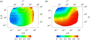
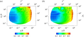
The convection velocity and correlation coefficient, (2.14) and (2.15), are presented in figure 5 at
 $\mathit{Re}_{{\it\theta}}=13\,000$
using the dispersion relation
 $2{\rm\pi}f=-k_{x}\,U_{c}(\,f)$
. Consistent with theory (Lin Reference Lin1953),
 ${\it\gamma}_{u}$
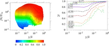
suggests that the validity of Taylor’s hypothesis is all the better as smaller structures are considered further away from the wall. Indeed, the length scale of the structure and the mean shear (which increases nearer the wall) are sources of anisotropy, whereas Taylor’s hypothesis originates in homogeneous isotropic turbulence. However, even the footprint of the largest length scales does not feature a correlation coefficient as low as the reported minima of del Álamo & Jiménez (Reference del Álamo and Jiménez2009) (the correlation coefficient definitions coincide in the dual cases). In figure 6,
 ${\it\gamma}_{u}(y;f)$
is plotted instead of
 ${\it\gamma}_{u}(y;{\it\lambda}_{x})$
. The variations of
 ${\it\gamma}_{u}$
for constant
 $f$
with respect to
 $y$
suggest that the small values corresponding to the largest scales very near the wall do not result from low-frequency resolution limitations from the finite-length signals, because these limitations depend only on
 $f$
, not on
 $y$
. The small
 ${\it\gamma}_{u}$
of the largest scales seem to be related to the flow physics instead, in agreement with Lin (Reference Lin1953), more specifically to the intermittency of these scales. Indeed, Buxton et al. (Reference Buxton, de Kat and Ganapathisubramani2013) report in a plane shear layer that the tail of distribution of the probability density of the convection velocity is larger for the largest scales, i.e. the convection velocity fluctuates more towards unexpected values, which is attributed to intermittency.
Convection velocity
 $U_{c}/U_{\infty }$
(coloured contours, a) and correlation coefficient
 ${\it\gamma}_{u}$
(coloured contours, b) at
 $\mathit{Re}_{{\it\theta}}=13\,000$
as a function of the wavelength and the wall distance. Solid lines are isolines of
 $k_{x}G_{uu}(k_{x})/u_{{\it\tau}}^{2}$
.

Correlation coefficient
 ${\it\gamma}_{u}$
(coloured contours) at
 $\mathit{Re}_{{\it\theta}}=13\,000$
as a function of the frequency and the wall distance. Solid lines are isolines of
 $k_{x}G_{uu}(k_{x})/u_{{\it\tau}}^{2}$
.

The outer-scaled convection velocity is presented in figure 5. The largest scales (around
 ${\it\lambda}_{x}=10\,{\it\delta}$
, associated with superstructures) have a relatively uniform convection velocity across the whole boundary layer thickness. This uniformity is a necessary condition for the coherence of the motion, as recalled in the Introduction. Near-wall confinement implies that very large-scale motions must extend to higher distances above the wall than smaller scales, where the mean velocity is larger, so that the largest scales are convected faster than the smaller scales near the wall. In figure 5 the footprint of the largest scales is indeed faster (consistent with Hutchins et al.
Reference Hutchins, Monty, Ganapathisubramani, Ng and Marusic2011) and their top is slower than the other structures.
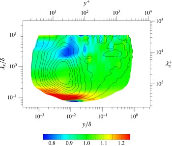
The convection velocity is compared with the mean velocity in figure 7(a). Near the wall, it is significantly larger than the mean velocity at all length scales. It is slightly smaller than the mean in the outer part of the outer layer, in good qualitative agreement with Favre et al. (Reference Favre, Gaviglio and Dumas1967), del Álamo & Jiménez (Reference del Álamo and Jiménez2009), Chung & McKeon (Reference Chung and McKeon2010), Lee & Sung (Reference Lee and Sung2011) and Atkinson et al. (Reference Atkinson, Buchmann and Soria2015), among others. However, the lack of datasets matching the present Reynolds number and type of flow prevents a direct comparison. The three energy sites (inner, outer in the range of scales of the hairpin packets, and outer superstructure site) feature a common property: the convection velocity is higher than the mean velocity near the foot of the site, and lower than the mean near the top of the site. This is especially consistent with del Álamo & Jiménez (Reference del Álamo and Jiménez2009) assessing the convection velocity in channel flow as the mean velocity averaged over the height of the structure.
Convection velocity divided by the mean streamwise velocity
 $U_{c}/\langle U\rangle$
(coloured contours, (a) and by the correlation-based convection velocity
 $U_{c}/U_{corr}$
(coloured contours, (b) at
 $\mathit{Re}_{{\it\theta}}=13\,000$
as a function of the wavelength and the wall distance. Black solid lines, isolines of
 $k_{x}G_{uu}(k_{x})/u_{{\it\tau}}^{2}$
; white solid line, line of equal convection velocity and mean velocity
 $U_{c}=\langle U\rangle$
.

Near the wall, even the small structures are convected much faster than the mean velocity. It is possible that their core is located higher in the boundary layer, where the mean velocity is larger, if the wall distance considered is smaller than the wall-normal extent of the structure. Another possible explanation derives from the amplitude modulation of the small-scale near-wall activity by the largest scales, which also superimpose their large-scale contribution to the velocity fluctuations (see Mathis et al. Reference Mathis, Hutchins and Marusic2011). Most of the small-scale energy is generated in the presence of large-scale positive velocity fluctuations because of the associated higher near-wall shear. Since the convection velocity (2.14) is evaluated from PSDs, it relies on energy-carrying events, so that it may be close to the velocity in the presence of large-scale positive velocity fluctuations, which is larger than the mean.
Figure 7 also depicts (white solid line) the locus where
 $U_{c}(\,f)=\langle U\rangle$
. This is, to some extent, reminiscent of the so-called critical layer associated with hydrodynamic instabilities, which is the height where the phase speed of a linear perturbation mode is equal to the mean velocity, a singularity for inviscid parallel shear flows. However, the critical layer is no longer singular in viscous parallel flows, and the maximum amplitude of the perturbation mode is not necessarily in the vicinity of this layer (Charru Reference Charru2011). Moreover, the present flow is not exactly parallel.
Finally, figure 7(b) compares the frequency-dependent convection velocity with the global correlation-based convection velocity
 $U_{corr}(y)$
which does not depend on frequency and has already been used in figure 4. Globally speaking, both velocities are close to each other. Near the wall, the largest scales are convected much faster than the smaller scales. The lower convection velocity of the extremely large wavelengths very near the wall is not significant, because of the low energy content of the signal at the largest length scales which leads to poor signal-to-noise ratios. Figure 7 will be further discussed in § 5.
4. Estimation of the spatial spectrum from the temporal spectrum
The frequency-dependent convection velocity may be used to reconstruct streamwise spectra from time signals (see the Introduction). This involves a dilatation factor, as introduced by del Álamo & Jiménez (Reference del Álamo and Jiménez2009) and Monty & Chong (Reference Monty and Chong2009), which is derived here for the present method.
4.1. Dilatation factor
Reconstruction of the streamwise PSD
 $S_{uu}(k_{x})$
from the estimated time PSD
 $S_{uu}(\,f)$
and the frequency-dependent convection velocity
 $U_{c}(\,f)$
(2.14), where the frequency and the streamwise wavenumber are related by the dispersion relation
 $2{\rm\pi}f=-U_{c}(\,f)\,k_{x}$
, must preserve the signal energy:
 $$\begin{eqnarray}\int _{-\infty }^{\infty }S_{uu}(\,f)\,\text{d}f=E(u^{2})=\int _{-\infty }^{\infty }S_{uu}(k_{x})\,\text{d}k_{x}.\end{eqnarray}$$
Seeing the dispersion relation as a change of variables, the following condition must hold:
 $$\begin{eqnarray}S_{uu}\left(k_{x}=-\frac{2{\rm\pi}f}{U_{c}(\,f)}\right)=S_{uu}(\,f)\left|\frac{\text{d}f}{\text{d}k_{x}(\,f)}\right|,\end{eqnarray}$$
where
 $|\text{d}f/\text{d}k_{x}(\,f)|$
is the absolute value of the Jacobian of the frequency–wavenumber transformation resulting from the dispersion relation
 $2{\rm\pi}f=-U_{c}(f(k_{x}))\,k_{x}$
. Deriving the latter relation with respect to
 $k_{x}$
leads to
 $$\begin{eqnarray}\frac{\text{d}f}{\text{d}k_{x}(\,f)}=\frac{1}{2{\rm\pi}}\frac{-U_{c}(\,f)}{\displaystyle 1+k_{x}\frac{\text{d}U_{c}(\,f)}{\text{d}(2{\rm\pi}f)}}=\frac{1}{2{\rm\pi}}\frac{-U_{c}(\,f)}{\displaystyle 1-\frac{2{\rm\pi}f}{U_{c}(\,f)}\frac{\text{d}U_{c}(\,f)}{\text{d}(2{\rm\pi}f)}}\quad (U_{c}(\,f)\neq 0).\end{eqnarray}$$
 $U_{c}(\,f)\neq 0$
is not a restrictive assumption, because the method is meant for time stationary spatially developing flows. Working in a frame of reference where the turbulent statistics are time stationary and where
 $U_{c}$
vanishes would contradict streamwise heterogeneity. Furthermore, reconstructing a streamwise fluctuation from its time signal is in fact impossible if it is convected at zero velocity. In the case of the boundary layer where the reference frame is the solid wall, all turbulent fluctuations are convected towards
 $x>0$
at
 $U_{c}(\,f)>0$
, but the general case is considered in the following.
From (4.3) and (4.2) and the dispersion relation, the pre-multiplied spectra are related as follows:
 $$\begin{eqnarray}k_{x}S_{uu}\left(k_{x}=-\frac{2{\rm\pi}f}{U_{c}(\,f)}\right)=fS_{uu}(\,f)\frac{-\text{sign}(U_{c}(\,f))}{\displaystyle \left|1-\frac{f}{U_{c}(\,f)}\frac{\text{d}U_{c}(\,f)}{\text{d}f}\right|}.\end{eqnarray}$$
For one-sided PSDs, only positive frequencies and wavenumbers are considered (e.g.
 $G_{uu}(\,f)$
represents both the contributions of
 $S_{uu}(\,f)$
and
 $S_{uu}(-f)=S_{uu}(\,f)$
). The frequency–wavenumber relation becomes
 $2{\rm\pi}f=|U_{c}(\,f)|\,k_{x}$
, and the pre-multiplied one-sided PSDs are related by the dilatation factor
 $$\begin{eqnarray}k_{x}G_{uu}\left(k_{x}=\frac{2{\rm\pi}f}{|U_{c}(\,f)|}\right)=fG_{uu}(\,f)\underbrace{\frac{1}{\displaystyle \left|1-\frac{f}{U_{c}(\,f)}\frac{\text{d}U_{c}(\,f)}{\text{d}f}\right|}}_{dilatation~factor}\end{eqnarray}$$
where we recall that
 $\int _{0}^{\infty }G_{uu}(k_{x})\,\text{d}k_{x}=E(u^{2})$
. The dilatation factor is a local energy-preservation correction to the pre-multiplied PSD taking into account the frequency dependence of
 $U_{c}(\,f)$
. When
 $U_{c}(\,f)$
does not vary with
 $f$
, this factor reduces to 1 and time and streamwise pre-multiplied PSDs are equal. The factor coincides with the ratio of the group velocity to the phase velocity defined from the dispersion relation, as mentioned in del Álamo & Jiménez (Reference del Álamo and Jiménez2009). The group velocity is discussed in § 7.
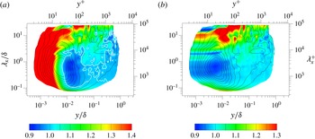
The dilatation factor defined by (4.5) is shown in figure 8. It is smaller than 1 between the inner site and the footprint of the superstructures. Indeed, the foot of the superstructures is advected faster than the surrounding structures. Since a given wavenumber advected at a higher convection velocity has a higher frequency, the wavenumber gap between both sites is wider than the frequency gap, so the PSD must be reduced to preserve the integral over this area. As for the values near the very largest and smallest wavelengths, they are dominated by noise in these low-energy regions, which is not an issue since it is only a correction factor to the PSD, which is in any case small. The dilatation factor is used in the next section to reconstruct the streamwise spectrum.
Dilatation factor (4.5) (coloured contours) at
 $\mathit{Re}_{{\it\theta}}=13\,000$
as a function of the wavelength and the wall distance. Solid lines are isolines of
 $k_{x}G_{uu}(k_{x})/u_{{\it\tau}}^{2}$
. The values at the largest wavelengths as well as at the smallest wavelengths should not be considered, because the energy in these regions is too low for a convenient signal-to-noise ratio to be achieved, leading to inaccuracies in the assessment of the dilatation factor.

4.2. Comparison of the reconstructed streamwise spectrum with classical strategies
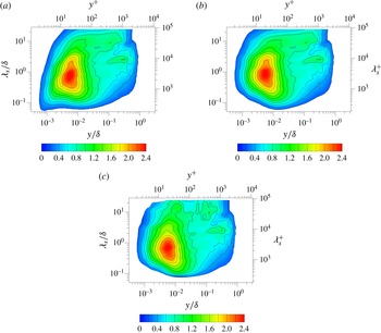
The streamwise spectrum is reconstructed from the frequency spectrum using (4.5). The convection velocity
 $U_{c}(\,f)$
is involved in the frequency-to-wavenumber transformation and in the dilatation factor. This is compared in figure 9 with two classical reconstruction strategies differing by the convection velocity definition, which does not depend on frequency (the dilation factor is unity). The mean velocity
 $U_{c}=\langle U\rangle$
is used in the first strategy, frequently found in experiments. The second strategy uses the correlation-based global convection velocity
 $U_{c}=U_{corr}$
, already mentioned previously and further discussed in § 5. The most significant variation is near the wall, where the convection velocity is significantly larger than the mean velocity, so that the first strategy (
 $U_{c}=\langle U\rangle$
) is very different from the others (
 $U_{c}=U_{corr}$
and
 $U_{c}(\,f)$
). The differences between the latter strategies, although
 $U_{c}(\,f)$
is based on a global value equivalent to
 $U_{corr}$
, as is demonstrated in § 5.2, illustrate the advantage of taking into account frequency dependence. First, the wavelength of the footprint of the superstructures is underestimated if a uniform convection velocity is used, as pointed out by del Álamo & Jiménez (Reference del Álamo and Jiménez2009) and observed in figure 9. Indeed, the footprint is convected faster than the other fluctuations near the wall, requiring an accurate frequency-to-wavenumber transformation (whereas the dilatation factor has little impact). Only with the frequency-dependent assessment is the wavelength of the energy site associated with the superstructures and their footprint constant across the boundary layer. A second effect, even though smaller, is related to the dilatation factor being smaller than unity between the inner site and the footprint of superstructures (figure 8). This results in a better circularity of the inner site in figure 9 compared with the spurious elongation of its large-wavelength edge when no frequency dependence is considered.
Pre-multiplied streamwise PSD
 $k_{x}G_{uu}(k_{x})/u_{{\it\tau}}^{2}$
estimated from the temporal spectrum at
 $\mathit{Re}_{{\it\theta}}=13\,000$
as a function of the wavelength and the wall distance: (a)
 $U_{c}=\langle U\rangle$
; (b)
 $U_{c}=U_{corr}$
; (c)
 $U_{c}=U_{c}(\,f)$
.

One may conclude that the main differences are located in the inner layer, where the correlation-based strategy strongly differs from the mean velocity. The improvements from the scale dependence are more subtle, so it is required only for a refined analysis of the spectrum, or to get physical insight into the turbulence dynamics through convection properties and the validity of Taylor’s hypothesis.
5. Defining a global convection velocity
The least-squares-based global convection velocity
 $C_{u}$
defined in § 2.1 takes into account all scales of motion. It will next be written as a weighted harmonic average of the frequency-dependent convection velocity
 $U_{c}(\,f)$
derived from
 $C_{u}$
in § 2.2, similar to the analysis of del Álamo & Jiménez (Reference del Álamo and Jiménez2009) in the dual case.
5.1. Global convection velocity and global correlation coefficient
The global convection velocity
 $C_{u}$
is expressed as a weighted harmonic average of its frequency-dependent counterpart
 $U_{c}(\,f)$
by inserting (2.14) into (2.10) and finally introducing one-sided power spectral densities (with factors 2 for
 $f>0$
cancelling out):
 $$\begin{eqnarray}C_{u}=\frac{\displaystyle \int _{0}^{\infty }f^{2}G_{uu}(\,f)\,\text{d}f}{\displaystyle \int _{0}^{\infty }\frac{1}{U_{c}(\,f)}f^{2}G_{uu}(\,f)\,\text{d}f},\end{eqnarray}$$
which is dual to equation (2.7) of del Álamo & Jiménez (Reference del Álamo and Jiménez2009).
From (2.12) and (2.14), one may rewrite the global correlation coefficient as
 $$\begin{eqnarray}{\it\gamma}_{u}=\frac{\displaystyle \left|\int _{0}^{\infty }\frac{1}{U_{c}(\,f)}(2{\rm\pi}f)^{2}G_{uu}(\,f)\,\text{d}f\right|}{\displaystyle \sqrt{\int _{0}^{\infty }(2{\rm\pi}f)^{2}G_{uu}(\,f)\,\text{d}f}\sqrt{\int _{0}^{\infty }G_{\partial _{x}u\,\partial _{x}u}(\,f)\,\text{d}f}}\end{eqnarray}$$
and, using (5.1),
 $$\begin{eqnarray}{\it\gamma}_{u}=\frac{1}{|C_{u}|}\sqrt{\frac{\displaystyle \int _{0}^{\infty }(2{\rm\pi}f)^{2}G_{uu}(\,f)\,\text{d}f}{\displaystyle \int _{0}^{\infty }G_{\partial _{x}u\,\partial _{x}u}(\,f)\,\text{d}f}},\end{eqnarray}$$
which is dual to equation (2.8) of del Álamo & Jiménez (Reference del Álamo and Jiménez2009).
Alternatively,
 ${\it\gamma}_{u}$
is written as a function of the frequency-dependent
 ${\it\gamma}_{u}(\,f)$
, inserting (2.15) into (2.12),
 $$\begin{eqnarray}{\it\gamma}_{u}=\frac{\displaystyle \left|\int _{0}^{\infty }\text{sign}(\text{Im}(S_{u\partial _{x}u}(\,f)))\,f\sqrt{G_{uu}(\,f)}\,\sqrt{G_{\partial _{x}u\partial _{x}u}(\,f)}\,{\it\gamma}_{u}(\,f)\,\text{d}f\right|}{\displaystyle \sqrt{\int _{0}^{\infty }f^{2}G_{uu}(\,f)\,\text{d}f}\sqrt{\int _{0}^{\infty }G_{\partial _{x}u\,\partial _{x}u}(\,f)\,\text{d}f}},\end{eqnarray}$$
which becomes
 $$\begin{eqnarray}{\it\gamma}_{u}=\frac{\displaystyle \left|\int _{0}^{\infty }\text{sign}(U_{c}(\,f))\,f\sqrt{G_{uu}(\,f)}\,\sqrt{G_{\partial _{x}u\partial _{x}u}(\,f)}\,{\it\gamma}_{u}(\,f)\,\text{d}f\right|}{\displaystyle \sqrt{\int _{0}^{\infty }f^{2}G_{uu}(\,f)\,\text{d}f}\sqrt{\int _{0}^{\infty }G_{\partial _{x}u\,\partial _{x}u}(\,f)\,\text{d}f}},\end{eqnarray}$$
noting in (2.14) that
 $\text{sign}(\text{Im}(S_{u\partial _{x}u}(\,f)))=-\text{sign}(fU_{c}(\,f))$
since
 $S_{uu}(\,f)\geqslant 0$
(
 $u(t)$
being statistically stationary). As discussed in § 4.1, one may assume that
 $U_{c}(\,f)$
does not vanish. The PSDs have been assumed to be continuous functions of
 $f$
in § 2.2, so
 $U_{c}(\,f)$
is also continuous. Consequently,
 $U_{c}(\,f)$
has a constant sign, and (5.5) becomes
 $$\begin{eqnarray}{\it\gamma}_{u}=\frac{\displaystyle \int _{0}^{\infty }\sqrt{f^{2}G_{uu}(\,f)}\,\sqrt{G_{\partial _{x}u\partial _{x}u}(\,f)}\,{\it\gamma}_{u}(\,f)\,\text{d}f}{\displaystyle \sqrt{\int _{0}^{\infty }f^{2}G_{uu}(\,f)\,\text{d}f}\sqrt{\int _{0}^{\infty }G_{\partial _{x}u\,\partial _{x}u}(\,f)\,\text{d}f}}\quad (U_{c}(\,f)\neq 0\;\forall f).\end{eqnarray}$$
This expression is new and was not derived, even in the dual case, by del Álamo & Jiménez (Reference del Álamo and Jiménez2009);
 ${\it\gamma}_{u}$
may be seen as a weighted average of the correlation coefficient
 ${\it\gamma}_{u}(\,f)$
over
 $f$
, similar to (5.1) for
 $U_{c}(\,f)$
, but this average is biased since
 $\int _{0}^{\infty }\!\sqrt{f^{2}G_{uu}(\,f)}\,\sqrt{G_{\partial _{x}u\partial _{x}u}(\,f)}\,\text{d}f\neq \sqrt{\int _{0}^{\infty }f^{2}G_{uu}(\,f)\,\text{d}f}\sqrt{\int _{0}^{\infty }G_{\partial _{x}u\,\partial _{x}u}(\,f)\,\text{d}f}$
a priori (unless
 $U_{c}(\,f)$
is constant over all
 $f$
).
The present global convection velocity
 $C_{u}$
(5.1) and the associated correlation coefficient (5.3) are shown in figure 10, together with the mean velocity and the correlation-based convection velocity
 $U_{corr}$
mentioned previously (and discussed in more detail in the next section). Consistent with the findings in the literature, the global convection velocity is close to the mean velocity, except near the wall where it is significantly larger and has a nearly constant value. In the outer layer, it is slightly smaller than the mean velocity. The global correlation coefficient has high values, especially in the outer layer, and decreases near the wall as predicted by Lin (Reference Lin1953).
Outer-scaled streamwise velocities
 $U/U_{\infty }$
at
 $\mathit{Re}_{{\it\theta}}=13\,000$
: mean velocity
 $\langle U\rangle$
, correlation-based convection velocity
 $U_{corr}$
, global convection velocity
 $C_{u}$
, and partially integrated global convection velocity (
 $C_{u}({\it\lambda}_{x}>4{\it\delta})$
and
 $C_{u}({\it\lambda}_{x}<4{\it\delta})$
). The associated correlation coefficients
 ${\it\gamma}_{u}$
are plotted on the right-hand axis.

The convection of the superstructures is isolated from the smaller structures in figure 10 considering only
 ${\it\lambda}_{x}/{\it\delta}\geqslant 4$
by partially integrating (5.1) and (5.3). The frequency range is determined from the wavenumber range using the dispersion relation
 $2{\rm\pi}f=-U_{c}(\,f)\,k_{x}$
and assuming that
 $k_{x}(\,f)$
is a monotonous function, which is the case because the variations of
 $U_{c}(\,f)$
are slow enough. The largest length scales (
 ${\it\lambda}_{x}/{\it\delta}\geqslant 4$
) are convected faster than the other scales near the wall, but the associated correlation coefficient is relatively low (consistent with Lin Reference Lin1953). There is very little difference between the convection velocity and correlation coefficient accounting for either all scales or those scales such that
 ${\it\lambda}_{x}/{\it\delta}\leqslant 4$
, suggesting that the contribution of the superstructures is not taken much into account through the weighted average process described by (5.1) and (5.6). This will be easily explained via the physical interpretation of
 $C_{u}$
given in § 6.2, revealing that the dissipative scales dominate its value, and incidentally emphasizing that the global profiles of
 $C_{u}$
and
 ${\it\gamma}_{u}$
(all scales) presented in figure 10 may depend on the resolution of the numerical simulation. In contrast, the values describing the largest scales only (
 ${\it\lambda}_{x}/{\it\delta}>4$
) do not directly depend on the resolution.
Furthermore,
 $C_{u}$
and
 $U_{corr}$
are very close to each other. A theoretical equivalence between both definitions in the limit of vanishing correlation separation for
 $U_{corr}$
is demonstrated in the next section. This suggests that the evaluation of
 $C_{u}$
, which could be altered by numerical errors from PSD estimations and discrete integration, is reliable because it coincides with
 $U_{corr}$
in agreement with theory (the correlation-based method features fewer sources of numerical errors). In turn, this validates the numerical assessment of
 $U_{c}(\,f)$
(because it determines
 $C_{u}$
), which cannot be done experimentally because no dataset is available at the same Reynolds number in the same flow. The theoretical equality between
 $U_{corr}$
and
 $C_{u}$
, which is demonstrated in the next section, suggests the interpretation of figure 7(b) as depicting the variations of
 $U_{c}(\,f)$
around its weighted frequency harmonic average
 $C_{u}$
.
5.2. Equivalence with the correlation-based convection velocity
The correlation-based convection velocity
 $U_{corr}$
mentioned in previous sections results from a linear fit to the relation between
 ${\rm\Delta}x$
and
 ${\it\tau}$
obtained by maximizing the correlation coefficient
 $(E(u(x,t)u(x+{\rm\Delta}x,t+{\it\tau}))/\sqrt{E(u(x,t)^{2})E(u(x+{\rm\Delta}x,t+{\it\tau})^{2})})$
over the time delay
 ${\it\tau}$
for five very small streamwise separations
 ${\rm\Delta}x$
(matching the mesh spacing) from the time signals stored at five successive mesh nodes. Wills (Reference Wills1964) recommends resorting to the correlation coefficient rather than to the correlation
 $E(u(x,t)u(x+{\rm\Delta}x,t+{\it\tau}))$
for streamwise heterogeneous flows. The smallest possible value
 ${\rm\Delta}x$
is used so that even the smallest shortest-lived structures are quasi-frozen over
 ${\it\tau}$
and
 $U_{corr}$
accounts for the convection of all scales. A dual method maximizing the coefficient over
 ${\rm\Delta}x$
for a given
 ${\it\tau}$
would not have been possible because the numerical constraints of the simulation lead to very small time step values compared with the streamwise mesh spacing and the convection velocity.
Figure 10 shows that
 $U_{corr}$
and the present global convection velocity
 $C_{u}$
(2.3) are very close to each other. This is explained here by demonstrating that minimizing
 $\mathscr{D}(C)=E(((1/C)\partial _{t}u+\partial _{x}u)^{2})/E((\partial _{x}u)^{2})$
over
 $C$
, which defines
 $C_{u}$
, is equivalent to maximizing the correlation coefficient
 $E(u(x,t)u(x+{\rm\Delta}x,t+{\it\tau}))/\sqrt{E(u(x,t)^{2})E(u(x+{\rm\Delta}x,t+{\it\tau})^{2})}$
over
 ${\it\tau}$
for a vanishing value of
 ${\rm\Delta}x$
, which defines
 $U_{corr}$
because the mesh spacing is very small. Indeed, the latter method is equivalent to maximizing
 $E(u(x,t)u(x+{\rm\Delta}x,t+{\rm\Delta}x/C))/\sqrt{E(u(x,t)^{2})E(u(x+{\rm\Delta}x,t+({\rm\Delta}x/C))^{2})}$
over the convection velocity
 $C$
for a given vanishing
 ${\rm\Delta}x$
(the time delay
 ${\it\tau}$
is
 ${\it\tau}={\rm\Delta}x/C$
). To second order in
 ${\rm\Delta}x$
, one may write
 $$\begin{eqnarray}\displaystyle u\left(x+{\rm\Delta}x,t+\frac{{\rm\Delta}x}{C}\right) & \mathop{=}_{{\rm\Delta}x\rightarrow 0} & \displaystyle u(x,t)+\left(\partial _{x}u+\frac{1}{C}\partial _{t}u\right){\rm\Delta}x\nonumber\\ \displaystyle & & \displaystyle +\left(\partial _{xx}u+\frac{2}{C}\partial _{xt}u+\frac{1}{C^{2}}\partial _{tt}u\right)\frac{{\rm\Delta}x^{2}}{2}+o({\rm\Delta}x^{2}),\end{eqnarray}$$
so it may be shown that the correlation coefficient becomes
 $$\begin{eqnarray}\displaystyle & & \displaystyle \frac{\displaystyle E\left(u(x,t)u\left(x+{\rm\Delta}x,t+\frac{{\rm\Delta}x}{C}\right)\right)}{\displaystyle \sqrt{E(u(x,t)^{2})E\left(u\left(x+{\rm\Delta}x,t+\frac{{\rm\Delta}x}{C}\right)^{2}\right)}}\nonumber\\ \displaystyle & & \displaystyle \quad \mathop{=}_{{\rm\Delta}x\rightarrow 0}1+\left(\frac{\displaystyle \left(E\left(u\left(\partial _{x}u+\frac{1}{C}\partial _{t}u\right)\right)\right)^{2}}{2(E(u^{2}))^{2}}-\frac{\displaystyle E\left(\left(\partial _{x}u+\frac{1}{C}\partial _{t}u\right)^{2}\right)}{2E(u^{2})}\right)(x,t)\nonumber\\ \displaystyle & & \displaystyle \qquad \quad \times \,{\rm\Delta}x^{2}+o({\rm\Delta}x^{2}).\end{eqnarray}$$
Assuming that the flow is statistically stationary, and since the mathematical expectation
 $E(\cdot )$
commutes with the time and space derivation (one of Reynolds’ axioms), we conclude that
 $E(u\,(1/C)\partial _{t}u)=(1/C)\partial _{t}E(u^{2}/2)=0$
, and that
 $E(u\partial _{x}u)=\partial _{x}E(u^{2}/2)$
. This leads to the final result, valid for a flow that is statistically stationary in time:
 $$\begin{eqnarray}\displaystyle & & \displaystyle \frac{\displaystyle E\left(u(x,t)u\left(x+{\rm\Delta}x,t+\frac{{\rm\Delta}x}{C}\right)\right)}{\displaystyle \sqrt{E(u(x,t)^{2})E\left(u\left(x+{\rm\Delta}x,t+\frac{{\rm\Delta}x}{C}\right)^{2}\right)}}\nonumber\\ \displaystyle & & \displaystyle \quad \mathop{=}_{{\rm\Delta}x\rightarrow 0}1+\left(\left(\frac{\partial _{x}E(u^{2})}{2E(u^{2})}\right)^{2}-\frac{\displaystyle E\left(\left(\partial _{x}u+\frac{1}{C}\partial _{t}u\right)^{2}\right)}{E(u^{2})}\right)(x)\times \frac{{\rm\Delta}x^{2}}{2}+o({\rm\Delta}x^{2}),\qquad\end{eqnarray}$$
from which it is concluded that maximizing the correlation coefficient
 $(E(u(x,t)u(x+{\rm\Delta}x,t+{\rm\Delta}x/C)))/\sqrt{E(u(x,t)^{2})E(u(x+{\rm\Delta}x,t+{\rm\Delta}x/C)^{2})}$
over
 $C$
for a given very small value of
 ${\rm\Delta}x$
, in the limit of vanishing
 ${\rm\Delta}x$
, is equivalent to the minimization of
 $E((\partial _{x}u+(1/C)\partial _{t}u)^{2})$
over
 $C$
, which is itself equivalent to the minimization of
 $\mathscr{D}(C)=E(((1/C)\partial _{t}u+\partial _{x}u)^{2})/E((\partial _{x}u)^{2})$
over
 $C$
. This shows that for a vanishing
 ${\rm\Delta}x$
,
 $U_{corr}$
and
 $C_{u}$
are equivalent, consistent with the observations in figure 10. The coexistence of the correlation-based and least-squares-minimized-residual definitions leads to two different physical interpretations given in the next section.
6. Physical interpretation of the present global convection velocity definition
In the next section, the correlation-based convection velocity
 $U_{corr}$
is interpreted as the initial velocity of a turbulence-freezing frame of reference. A second section then interprets the equivalent global convection velocity
 $C_{u}$
, defined in the present study via the minimization of the convection equation mean-squared residual, in terms of turbulence micro scale maximization in a convected frame of reference.
6.1. Initial velocity of a turbulence-freezing frame of reference
The convection velocity
 $U_{corr}$
described previously is related to a broad category of velocities defined by maximizing the correlation
 $R_{uu}({\rm\Delta}x,{\it\tau})=E(u(x,t)u(x+{\rm\Delta}x,t+{\it\tau}))$
. While
 $U_{corr}$
relies on a maximization over
 ${\it\tau}$
for a given
 ${\rm\Delta}x$
, the most intuitive physical interpretation of these methods is obtained in the dual case of a maximization over
 ${\rm\Delta}x$
for a given
 ${\it\tau}$
, which is treated first.
Defining the value
 ${\rm\Delta}x_{max}({\it\tau})$
of
 ${\rm\Delta}x$
that maximizes
 $R_{uu}({\rm\Delta}x,{\it\tau})$
for a given
 ${\it\tau}$
, one notices that
 $R_{uu}({\rm\Delta}x_{max}({\it\tau}),{\it\tau})$
coincides with the time correlation in a frame of reference that is moving such that its origin at time
 ${\it\tau}$
has the streamwise coordinate
 ${\rm\Delta}x_{max}({\it\tau})$
. Fisher & Davies (Reference Fisher and Davies1963) and Wills (Reference Wills1964) point out that in this frame of reference, the correlation decays as slowly as possible in time, by definition of
 ${\rm\Delta}x_{max}({\it\tau})$
. The classical convection velocity defined as the ratio
 ${\rm\Delta}x_{max}({\it\tau})/{\it\tau}$
and which depends on
 ${\it\tau}$
may be seen as the mean velocity of this frame of reference during the time
 ${\it\tau}$
. The frame is not necessarily inertial, because its instantaneous velocity
 $\text{d}({\rm\Delta}x_{max}({\it\tau}))/\text{d}{\it\tau}$
may vary in time. Favre et al. (Reference Favre, Gaviglio and Dumas1967) consider the value of
 $\text{d}({\rm\Delta}x_{max}({\it\tau}))/\text{d}{\it\tau}$
at a given time
 ${\it\tau}$
as another possible definition of the convection velocity (but this is done in a mathematical way, with no reference to the instantaneous velocity of a moving frame). Furthermore, Favre et al. (Reference Favre, Gaviglio and Dumas1967) show that if the flow is homogeneous along
 $x$
, both mean and instantaneous velocities coincide when
 ${\it\tau}$
vanishes, and are given by
 $$\begin{eqnarray}\lim _{{\it\tau}\rightarrow 0}\frac{{\rm\Delta}x_{max}({\it\tau})}{{\it\tau}}({\it\tau})=\lim _{{\it\tau}\rightarrow 0}\frac{\text{d}({\rm\Delta}x_{max}({\it\tau}))}{\text{d}{\it\tau}}({\it\tau})=-\frac{E(\partial _{t}u\partial _{x}u)}{E(\partial _{x}u\partial _{x}u)}.\end{eqnarray}$$
The latter expression from Favre et al. (Reference Favre, Gaviglio and Dumas1967) coincides with equation (2.4) of del Álamo & Jiménez (Reference del Álamo and Jiménez2009), even though the derivations are different. The global convection velocity of del Álamo & Jiménez (Reference del Álamo and Jiménez2009) may be interpreted, based on Favre et al. (Reference Favre, Gaviglio and Dumas1967), as the initial velocity of a moving frame in which the correlation decays as slowly as possible in time (turbulence is frozen), assuming streamwise homogeneity.
As mentioned in § 5.2, the present dataset requires dual definitions, all the more as the flow is spatially developing. With the value
 ${\it\tau}_{max}({\rm\Delta}x)$
of
 ${\it\tau}$
that maximizes
 $R_{uu}({\rm\Delta}x,{\it\tau})$
for a given
 ${\rm\Delta}x$
,
 $R_{uu}({\rm\Delta}x,{\it\tau}_{max}({\rm\Delta}x))$
coincides with the time correlation in a frame of reference that is moving such that its origin reaches the streamwise position
 ${\rm\Delta}x$
at time
 ${\it\tau}_{max}({\rm\Delta}x)$
. By definition of
 ${\it\tau}_{max}({\rm\Delta}x)$
, this ensures the slowest possible spatial decay of the correlation. The classically defined convection velocity
 ${\rm\Delta}x/{\it\tau}_{max}({\rm\Delta}x)$
is seen as the (time) average velocity of this frame of reference over
 ${\rm\Delta}x$
(on which it depends). Similarly to the dual case, the instantaneous velocity of the frame
 $\text{d}({\rm\Delta}x)/\text{d}({\it\tau}_{max}({\rm\Delta}x))$
depends on
 ${\rm\Delta}x$
and may be used as a convection velocity (as did Favre et al.
Reference Favre, Gaviglio and Dumas1967 mathematically). Favre et al. (Reference Favre, Gaviglio and Dumas1967) show that as soon as the flow is statistically stationary (in time, since no spatial homogeneity is required for their derivation), both mean and instantaneous velocities coincide when
 ${\rm\Delta}x$
vanishes, and are given by
 $$\begin{eqnarray}\lim _{{\rm\Delta}x\rightarrow 0}\frac{{\rm\Delta}x}{{\it\tau}_{max}({\rm\Delta}x)}({\rm\Delta}x)=\lim _{{\rm\Delta}x\rightarrow 0}\frac{\text{d}({\rm\Delta}x)}{\text{d}({\it\tau}_{max}({\rm\Delta}x))}({\rm\Delta}x)=-\frac{E(\partial _{t}u\partial _{t}u)}{E(\partial _{t}u\partial _{x}u)}(x).\end{eqnarray}$$
The latter expression from Favre et al. (Reference Favre, Gaviglio and Dumas1967) coincides with the global convection velocity
 $C_{u}$
defined in (2.3). This relation between the velocity
 $C_{u}$
(2.3) minimizing the squared residual expectation and the limit of the convection velocity maximizing the correlation for a given
 ${\rm\Delta}x$
is consistent with the previous direct demonstration that
 $C_{u}$
also coincides with
 $U_{corr}$
defined by maximizing the correlation coefficient (instead of the correlation) for a vanishing
 ${\rm\Delta}x$
.
 $C_{u}$
and
 $U_{corr}$
for a vanishing
 ${\rm\Delta}x$
are interpreted as the initial velocity of the moving frame of reference that provides the slowest spatial decay of the correlation, i.e. turbulence is frozen over the longest possible distance, with no other assumption than statistical time stationarity.
6.2. Turbulence micro scale maximization in a convected frame of reference
The present global convection velocity
 $C_{u}$
(2.3) minimizes the expectation of the squared residual of the convection equation
 $E(((1/C)\partial _{t}u+\partial _{x}u)^{2})$
. This mathematical definition coincides with the phase velocity in the non-fluctuating convection of a single Fourier mode (see the Introduction, (1.16)). A physical interpretation for a broadband turbulence signal with fluctuating convection velocity, which is lacking in the literature known to the authors, is proposed here.
The interpretation is set in a convected inertial frame of reference with streamwise and time coordinates
 $(x_{c}=x-Ct,t)$
, moving at a constant velocity
 $C$
along
 $x$
with respect to the usual frame of reference with coordinates
 $(x,t)$
where the wall is still. The expectation
 $E$
is seen as a spanwise and ensemble average so that it is a Reynolds average
 $\langle \cdot \rangle$
in both frames, commuting with derivatives. The streamwise velocity
 $U$
in the usual frame becomes
 $U-C$
in the convected frame. The velocity fluctuation
 $u=U-\langle U\rangle$
and its variance
 $E(u^{2})$
are the same in both frames because
 $C$
is constant. The partial time derivative in the convected frame
 $(\partial u/\partial t)_{x_{c}}$
is a function of the partial time and streamwise derivatives in the usual frame,
 $$\begin{eqnarray}\left(\frac{\partial u}{\partial t}\right)_{x_{c}}=\left(\frac{\partial u}{\partial t}\right)_{x}\left(\frac{\partial t}{\partial t}\right)_{x_{c}}+\left(\frac{\partial u}{\partial x}\right)_{t}\left(\frac{\partial x}{\partial t}\right)_{x_{c}}=\left(\frac{\partial u}{\partial t}\right)_{x}+\left(\frac{\partial u}{\partial x}\right)_{t}C\end{eqnarray}$$
so that the expectation of the squared residual becomes
 $$\begin{eqnarray}E\left(\left(\frac{1}{C}\partial _{t}u+\partial _{x}u\right)^{2}\right)=\frac{1}{C^{2}}E\left(\left(\frac{\partial u}{\partial t}\right)_{x_{c}}^{2}\right),\end{eqnarray}$$
which will now be related to the temporal auto-correlation of
 $u$
in the convected frame, defined as
 $$\begin{eqnarray}\displaystyle R_{uu}^{c}(x_{c},t;{\it\tau}) & = & \displaystyle E(u(x_{c},t)u(x_{c},t+{\it\tau}))\nonumber\\ \displaystyle & = & \displaystyle E(u(x=x_{c}+Ct,t)u(x+{\rm\Delta}x=x_{c}+C(t+{\it\tau}),t+{\it\tau})).\end{eqnarray}$$
Since
 ${\it\tau}$
is independent from the space and time variables, one obtains
 $$\begin{eqnarray}\displaystyle \frac{\text{d}^{2}R_{uu}^{c}(x_{c},t;{\it\tau})}{\text{d}{\it\tau}^{2}} & = & \displaystyle E(u(x_{c},t)(\partial _{tt}u(x_{c},t+{\it\tau}))_{x_{c}})\nonumber\\ \displaystyle & \Rightarrow & \displaystyle \frac{\text{d}^{2}R_{uu}^{c}(x_{c},t;0)}{\text{d}{\it\tau}^{2}}=E(u(x_{c},t)(\partial _{tt}u(x_{c},t))_{x_{c}}),\end{eqnarray}$$
 $$\begin{eqnarray}\displaystyle \frac{\text{d}^{2}R_{uu}^{c}(x_{c},t;0)}{\text{d}{\it\tau}^{2}} & = & \displaystyle (\partial _{tt}E(u(x_{c},t)^{2}/2))_{x_{c}}-E((\partial _{t}u(x_{c},t))_{x_{c}}^{2}).\end{eqnarray}$$
 $(\partial _{tt}E(u(x_{c},t)^{2}/2))_{x_{c}}=C^{2}\,(\partial _{xx}E(u(x_{c},t)^{2}/2))_{t}$
, which leads, together with (6.4) and (6.7), to the relation
 $$\begin{eqnarray}E\left(\left(\frac{1}{C}\partial _{t}u+\partial _{x}u\right)^{2}\right)=(\partial _{xx}E(u^{2}/2))_{t}-\frac{1}{C^{2}}\frac{\text{d}^{2}R_{uu}^{c}(x_{c},t;0)}{\text{d}{\it\tau}^{2}}.\end{eqnarray}$$
The global convection velocity is defined by the minimization over
 $C$
of
 $\mathscr{D}(C)=(E(((1/C)\partial _{t}u+\partial _{x}u)^{2}))/E((\partial _{x}u)^{2})$
, or equivalently of
 $\mathscr{E}(C)=(E(((1/C)\partial _{t}u+\partial _{x}u)^{2}))/2E(u^{2})$
, rewritten from (6.8):
 $$\begin{eqnarray}\mathscr{E}(C)=\frac{(\partial _{xx}E(u^{2}/2))_{t}}{2E(u^{2})}-\frac{\displaystyle \frac{\text{d}^{2}R_{uu}^{c}(x_{c},t;0)}{\text{d}{\it\tau}^{2}}}{2C^{2}E(u^{2})}=\underbrace{\frac{(\partial _{xx}E(u^{2}/2))_{t}}{2E(u^{2})}}_{independent\,of\,C}+\underbrace{\frac{\displaystyle -\frac{\text{d}^{2}R_{uu}^{c}}{\text{d}{\it\tau}^{2}}(x_{c},t;0)}{2C^{2}R_{uu}^{c}(x_{c},t;0)}}_{\mathscr{F}(C)}.\end{eqnarray}$$
Minimizing
 $\mathscr{D}(C)$
is equivalent to minimizing
 $\mathscr{F}(C)=1/(C^{2}{\it\tau}_{c}^{2})$
over
 $C$
, where the Eulerian micro time scale in the convected frame of reference
 ${\it\tau}_{c}$
is defined by (see Hinze Reference Hinze1959)
 $$\begin{eqnarray}\frac{\displaystyle -\frac{\text{d}^{2}R_{uu}^{c}}{\text{d}{\it\tau}^{2}}(x_{c},t;0)}{2R_{uu}^{c}(x_{c},t;0)}=\frac{1}{{\it\tau}_{c}^{2}}.\end{eqnarray}$$
Note that in the particular case when streamwise homogeneity is assumed in addition to statistical time stationarity, the flow is also time stationary in the convected frame (and homogeneous along
 $x_{c}$
). In this case,
 ${\it\tau}_{c}$
is the time delay
 ${\it\tau}$
when the osculating parabola to
 $R_{uu}^{c}(x_{c},t;{\it\tau})$
at
 ${\it\tau}=0$
reaches a zero correlation.
Coming back to the general case, the global convection velocity
 $C_{u}$
(2.3) is interpreted as the value of
 $C$
maximizing the length scale
 ${\it\lambda}_{c}=|C|{\it\tau}_{c}$
, corresponding to the distance travelled by the convected frame during a time equal to the Eulerian micro time scale of turbulence
 ${\it\tau}_{c}$
in this convected frame, i.e. the distance over which the coherence of turbulent fluctuations in the micro scale sense is preserved by following their convection. This interpretation applies to the equivalent correlation-based velocity
 $U_{corr}$
(see § 5.2), which is frequently used experimentally with a vanishing streamwise separation between two probes.
In the dual case of del Álamo & Jiménez (Reference del Álamo and Jiménez2009),
 $(E((\partial _{t}u+C\partial _{x}u)^{2})/E((\partial _{t}u)^{2}))=C^{2}\mathscr{D}(C)(E((\partial _{x}u)^{2})/E((\partial _{t}u)^{2}))$
is minimized instead of
 $\mathscr{D}(C)=(E(((1/C)\partial _{t}u+\partial _{x}u)^{2})/E((\partial _{x}u)^{2}))$
. Equivalently
 $C^{2}\mathscr{E}(C)$
is minimized over
 $C$
. From (6.9) multiplied by
 $C^{2}$
, one may conclude that a physical interpretation is also possible, but only assuming streamwise homogeneity of the flow (consistent with the requirements of the dual method, and similar to the time stationarity required for the present method). With this assumption, the method of del Álamo & Jiménez (Reference del Álamo and Jiménez2009) minimizes
 $C^{2}\mathscr{F}(C)$
, i.e. maximizes the micro time scale
 ${\it\tau}_{c}$
in the convected frame, which is more intuitive than maximizing
 ${\it\lambda}_{c}$
in the present method but requires streamwise homogeneity.
The maximization of the micro scale is reminiscent of another method to assess the convection velocity maximizing the integral scale, in a convected inertial frame of reference, using correlations computed for all possible values of both streamwise and time separations (see Fisher & Davies Reference Fisher and Davies1963; Wills Reference Wills1964). This is not suited to the present case especially because spatial growth of the boundary layer requires a local (in
 $x$
) formulation. Putting the emphasis on the large scales through the integral scale may also be irrelevant considering the validity of Taylor’s hypothesis for the largest near-wall scales (Lin Reference Lin1953), whereas
 $C_{u}$
, in contrast, is dominated by the small dissipative scales related to the micro scale. As demonstrated in § 5.1, the convection of the largest scales may still be isolated since the method is spectral.
The relation between the present global convection velocity
 $C_{u}$
and the micro scale is emphasized by the weight
 $f^{2}G_{uu}(\,f)$
in (5.1) for the weighted harmonic average giving
 $C_{u}$
from
 $U_{c}(\,f)$
, confirming that
 $C_{u}$
and
 $U_{corr}$
are dominated by the dissipative scales and explaining the results of figure 10 for the smaller-scale-restricted convection velocity. This, however, implies that
 $C_{u}$
and
 $U_{corr}$
(massively used in experiments) are dominated by the smallest resolved scales, which are not necessarily the dissipative scales if an under-resolved simulation or experiment is considered, possibly explaining some discrepancies between datasets of different resolution (see e.g. a comparison in LeHew et al.
Reference LeHew, Guala and McKeon2011) if the convection velocity of the dissipative scales and of larger scales is different. This suggests that a safe way of comparing convection velocities from different datasets, other than DNS or very well-resolved experiments, is to resort to the partial integration of
 $C_{u}$
(5.1) limited to frequencies suitably resolved by all datasets. This emphasizes the advantage of the spectral convection velocity compared with the correlation-based definition, all the more as their global values coincide (§ 5.2).
7. Assessment of the group velocity
From the dispersion relation
 $2{\rm\pi}f=-U_{c}(\,f)\,k_{x}$
, if
 $U_{c}(\,f)$
is considered as the phase velocity (consistent with the non-fluctuating monochromatic case described in the Introduction), one may define the associated group velocity
 $$\begin{eqnarray}v_{g}(\,f)=-\frac{\text{d}(2{\rm\pi}f)}{\text{d}k_{x}},\end{eqnarray}$$
where the minus sign ensures that
 $v_{g}(\,f)>0$
corresponds to the energy being conveyed towards
 $x>0$
, as will be justified below. From (4.3) we obtain the following result:
 $$\begin{eqnarray}v_{g}(\,f)=\frac{U_{c}(\,f)}{\displaystyle 1-\frac{f}{U_{c}(\,f)}\frac{\text{d}U_{c}(\,f)}{\text{d}f}}.\end{eqnarray}$$
The meaning of the group velocity is briefly restated here in keeping with chapter 3 of Charru (Reference Charru2011). A wavepacket is considered, with a spectral content centred on frequency
 $f_{0}$
and narrow enough for the dispersion relation to be linearized around frequency
 $f_{0}$
with satisfying accuracy,
 $$\begin{eqnarray}u(x,t)=2\text{Re}\left(\int _{0}^{\infty }\tilde{u} (\,f)\exp (2\text{i}{\rm\pi}ft+\text{i}k_{x}(\,f)x)\,\text{d}f\right),\end{eqnarray}$$
where
 $\tilde{u} (\,f)\exp (\text{i}k_{x}(\,f)x)$
is the time Fourier transform of
 $u(x,t)$
, which has the form of a complex exponential as a consequence of the assumption that the dispersion relation
 $2{\rm\pi}f=-U_{c}(\,f)\,k_{x}(\,f)$
is verified, and use has been made of the property
 $\tilde{u} (-f)\exp (\text{i}k_{x}(-f)x)=(\tilde{u} (\,f)\exp (\text{i}k_{x}(\,f)x))^{\ast }$
. To first-order accuracy in the width of the frequency band where the spectral content of
 $u(x,t)$
is concentrated, the dispersion relation may be written as
 $$\begin{eqnarray}k_{x}(\,f)\mathop{=}_{f-f_{0}\rightarrow 0}k_{x}(f_{0})-\frac{2{\rm\pi}}{v_{g}(f_{0})}(f-f_{0})+o(f-f_{0}),\end{eqnarray}$$
so that to first order in the frequency width around
 $f_{0}$
, the wavepacket may be approximated by
 $$\begin{eqnarray}\displaystyle u(x,t) & = & \displaystyle 2\text{Re}\left(\int _{0}^{\infty }\tilde{u} (\,f)\exp \left(2\text{i}{\rm\pi}ft+\text{i}\left(k_{x}(f_{0})-\frac{2{\rm\pi}}{v_{g}(f_{0})}(f-f_{0})\right)x\right)\,\text{d}f\right),\end{eqnarray}$$
 $$\begin{eqnarray}\displaystyle u(x,t) & = & \displaystyle 2\text{Re}\left(\underbrace{\exp \left(2\text{i}{\rm\pi}f_{0}t+\text{i}k_{x}(f_{0})x\right)}_{carrier\,wave}\right.\nonumber\\ \displaystyle & & \displaystyle \left.\times \,\underbrace{\int _{0}^{\infty }\tilde{u} (\,f)\exp \left(2\text{i}{\rm\pi}(f-f_{0})t-\text{i}\frac{2{\rm\pi}}{v_{g}(f_{0})}(f-f_{0})x\right)\,\text{d}f}_{A(x,t)}\right)\end{eqnarray}$$
 $A(x,t)$
is the envelope amplitude-modulating the carrier wave, verifying the property
 $$\begin{eqnarray}A(x,t)=A(x-v_{g}(f_{0})t,0).\end{eqnarray}$$
To first-order accuracy in the width of the frequency content around
 $f_{0}$
, the envelope of the wavepacket is moving at velocity
 $v_{g}(f_{0})$
without changing shape. Since the amplitude of the envelope determines whether or not the carrier wave contains energy, the group velocity
 $v_{g}(\,f)$
is thus the velocity at which the energy associated with a wavepacket narrowly concentrated around frequency
 $f$
and verifying the dispersion relation exactly is propagating downstream. Equation (7.7) confirms that
 $v_{g}(\,f)>0$
corresponds to the propagation of energy towards
 $x>0$
(hence the minus sign in (7.1)).
The resulting group velocity is compared with the phase velocity in figure 11. Little difference between the two velocities is shown by this figure. This is very consistent with the dilatation factor presented in § 4.1 being close to 1, so that the ratio between group and phase velocity is close to 1 as well.
Convection velocity
 $U_{c}/U_{\infty }$
(a) and group velocity
 $v_{g}/U_{\infty }$
(b) at
 $\mathit{Re}_{{\it\theta}}=13\,000$
as a function of the wavelength and the wall distance. Solid lines are isolines of
 $k_{x}G_{uu}(k_{x})/u_{{\it\tau}}^{2}$
.

The so-called phase velocity
 $U_{c}(\,f)$
does correspond to the phase velocity when pure convection is involved (see the Introduction), and has a mathematical interpretation (least-squares minimization of the convection equation residual) and a physical interpretation (micro time scale maximization, initial velocity of a freezing frame) when Taylor’s hypothesis is not perfectly valid. As for the group velocity, its classical interpretation relates to the propagation of the energy associated with the wavepacket that represents the coherent motion. The phase velocity might be irrelevant because the carrier, even though travelling at
 $U_{c}(\,f)$
, may omit the amplitude associated with the envelope travelling at
 $v_{g}(\,f)$
. This suggests that the group velocity could better describe the convection speed of a type of coherent motion, but three major drawbacks arise in turbulent flows.
First, the derivation assumes that the dispersion relation is exactly verified, but the convection velocity fluctuates and the validity of Taylor’s hypothesis is limited, so that only a strong approximation to Navier–Stokes equations is used. The group velocity is not defined from the exact wave equation describing the problem, and energy may be conveyed at a different speed.
Second, the group velocity is all the more relevant as there exist wavepackets, i.e. coherent motions, of very narrow frequency content (the group velocity derivation being first-order accurate in the frequency width). This is not the case for typical coherent motions because of the nonlinearity of Navier–Stokes equations. One coherent motion entails not only wavelengths close to its size, but also harmonics accounting for its non-sinusoidal shape and making the frequency band where the energy of the structure is located too broad for the group velocity derivation to be accurate enough.
The third drawback is that the narrower the frequency content of the wavepacket around
 $f_{0}$
, the wider the time signal spreads (because of the properties of the Fourier transform). This means that the observed size of the packet in the time signal may be associated with the characteristic time of the amplitude modulation, i.e. the inverse of the small bandwidth of its spectral content, and not with
 $1/f_{0}$
, which is related to the period of the carrier wave. Consequently,
 $v_{g}(f_{0})$
may be related to the propagation speed of an object, i.e. the narrow (in frequency) wavepacket, whose size is not related to
 $1/f_{0}$
. In contrast,
 $U_{c}(f_{0})$
seems to be related to the perturbations whose characteristic time is close to
 $1/f_{0}$
. For all these reasons, the use of
 $U_{c}(\,f)$
has been preferred over
 $v_{g}(\,f)$
in the present study.
8. Conclusion
The wavelength-dependent convection velocity of large-eddy-simulation-resolved streamwise velocity fluctuations has been assessed in a zero-pressure-gradient smooth flat plate turbulent boundary layer across the whole boundary layer profile at
 $\mathit{Re}_{{\it\theta}}=13\,000$
. The Reynolds number is high enough for the convection of superstructures to be observed, but the extreme computational cost of the simulation is out of reach of the published subsonic DNS datasets, so that a WRLES has been used, resorting to the zonal detached eddy simulation (ZDES) mode 3 technique and validated in Deck et al. (Reference Deck, Renard, Laraufie and Weiss2014b
).
As no existing method would satisfactorily address the spatial growth of the boundary layer and the data storage implied by the high Reynolds number while enabling a thorough physical interpretation of the obtained values, a new spectral method has been derived in the present study. It is inspired by the method of del Álamo & Jiménez (Reference del Álamo and Jiménez2009), which has great potential for interpretation when Taylor’s hypothesis is not rigorously valid, but whose input is spectral data and which assumes streamwise homogeneity (only the first steps of the derivation of a method suited to spatially developing flows were suggested). The new method assesses the frequency-dependent convection velocity from finite duration time signals (from which only power spectral density estimates may be obtained, not Fourier modes) and their local streamwise derivative, and it is suited to spatially developing flows. The validity of Taylor’s hypothesis is assessed using a correlation coefficient that coincides with the dual one of del Álamo & Jiménez (Reference del Álamo and Jiménez2009).
The results concerning the scale-dependent convection velocity suggest common features of the convection of near-wall structures, hairpin packets and superstructures. The high convection velocity associated with the near-wall footprint of the superstructures is clearly visible. Further, a remarkable trend in the validity of Taylor’s hypothesis has been reported, agreeing with theoretical predictions by Lin (Reference Lin1953). Consistent with del Álamo & Jiménez (Reference del Álamo and Jiménez2009), the streamwise spectrum has been reconstructed from the time spectrum by means of the frequency-dependent convection velocity, and compared with two classical strategies, where the convection velocity is either the mean velocity (which is common in experimental reconstruction of spectra) or a correlation-based non-scale-dependent velocity. The need for scale dependence depends on the main focus and refinement of the study.
The convection velocity has been interpreted as the phase velocity in the case of the non-fluctuating convection of a single Fourier mode, and in the general case as the minimization of the convection equation residual, consistent with del Álamo & Jiménez (Reference del Álamo and Jiménez2009). In addition, new physical interpretations have been given, including when Taylor’s hypothesis is not rigorously valid. One involves the initial velocity of a turbulence-freezing moving frame of reference, while the other is related to the maximization of the turbulence micro scales in a convected frame of reference. These interpretations also apply to the classical convection velocity that maximizes the two-point two-time correlation for a vanishing separation, typically used in experiments, which has been demonstrated to be equivalent to the present global convection velocity accounting for all scales and seen as a weighted harmonic average of the frequency-dependent convection velocity. This establishes connections between several methods existing in the literature and connects the present method to them.
Moreover, the global correlation coefficient (validity of Taylor’s hypothesis) has been newly described as a weighted average of the frequency-dependent correlation coefficient. Isolating the contribution of a scale band to the global velocity and correlation coefficient is very natural. The physical interpretation has been carried further by assessing and discussing the group velocity, which is not retained because of the nonlinearity of Navier–Stokes equations. In addition to the present method and the method of del Álamo & Jiménez (Reference del Álamo and Jiménez2009), four other methods have been proposed, which have not yet been used to the authors’ knowledge.
The present global convection velocity is dominated by the dissipative scales, which implies that a direct numerical simulation of the same test case would be very useful. It is also concluded that the correlation-based assessment of the convection velocity from experiments may similarly depend on the probe resolution. The present method not only adds the scale dependence description level, but also enables the rejection of the smallest scales when assessing the global convection velocity. This could be a way of comparing datasets with different degrees of resolution.
The study of convection velocity may be seen as an additional approach to coherent motions at high Reynolds numbers. Coherent motions are associated not only with a spectral energy site, but also with an almost uniform convection velocity zone, as explained by del Álamo & Jiménez (Reference del Álamo and Jiménez2009) and illustrated here. The study would be enhanced by simulations at even higher Reynolds numbers with clearer scale separation. Using this method to assess the physical validity of resolved motions in a WMLES might also be of interest.
Acknowledgements
This work was performed using HPC resources from GENCI-CINES (Project ZDESWALLTURB, grant 2012-[c2012026817]). The authors wish to thank P. Sagaut, P.-É. Weiss, R. Laraufie and L. Larchevêque for fruitful discussions. All the people involved in the evolution of the FLU3M code are warmly acknowledged. The thesis of N.R. is partly funded by the French defence procurement agency DGA.
Appendix A. On the choice of the minimized quantity defining the convection velocity
$C_{u}$

The present global convection velocity
 $C_{u}$
(2.3) minimizes
 $\mathscr{D}(C)=E(((1/C)\partial _{t}u+\partial _{x}u)^{2})/E((\partial _{x}u)^{2})$
over
 $C$
. The dual study by del Álamo & Jiménez (Reference del Álamo and Jiménez2009) instead minimized
 $E((\partial _{t}u+C\partial _{x}u)^{2})/E((\partial _{t}u)^{2})$
. The emphasis is placed on either time derivatives (present) or streamwise derivatives (del Álamo & Jiménez Reference del Álamo and Jiménez2009) depending on the available signal. Table 2 presents the expressions of
 $C_{u}$
minimizing three different functions
 $\mathscr{D}(C)$
(only if
 $C>0$
for definition #3 because
 $E((\partial _{t}u+C\partial _{x}u)((1/C)\partial _{t}u+\partial _{x}u))=E((1/C)(\partial _{t}u+C\partial _{x}u)^{2})$
), obtained from the condition
 $(\partial \mathscr{D}/\partial C)(C_{u})=0$
. All involve the expectation of the squared residual of the convection equation, written as either
 $\partial _{t}u+U_{c}\partial _{x}u=0$
or
 $(1/U_{c})\partial _{t}u+\partial _{x}u=0$
and normalized using the derivative term that does not depend on
 $C$
. The velocity
 $C_{u}(\#3)$
resulting from the space–time symmetrical definition #3 is the geometric mean
 $\sqrt{C_{u}(\#1)C_{u}(\#2)}$
of the velocities from the first two definitions, coinciding with the symmetrical velocity
 $V_{G}$
derived by Favre et al. (Reference Favre, Gaviglio and Dumas1967) from different considerations.
Possible convection velocity
 $C_{u}$
definitions, depending on the chosen quantity
 $\mathscr{D}(C)$
that is minimized over
 $C$
for
 $C=C_{u}$
. Associated correlation coefficient
 ${\it\gamma}_{u}$
. Spectral and global assessment of the convection velocity depending on the signal available (time or space). References when available (n.a., not available in the literature to the authors’ knowledge). Definition #3 assumes
 $C>0$
,
 $C_{u}>0$
, and in addition
 $f>0$
in the time signal lines,
 $k_{x}>0$
in the streamwise signal lines (time and streamwise signal lines should not be read simultaneously). Sign conventions are from (1.1) (
 $U_{c}>0$
for convection towards
 $x>0$
), (1.2) and (1.3), leading to the dispersion relation
 $2{\rm\pi}f=-U_{c}\,k_{x}$
. When using time signals, statistical stationarity is assumed. When using streamwise signals, streamwise homogeneity is assumed.
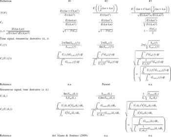
In a similar way to § 2.2, PSDs are used to derive a scale-dependent convection velocity and to write the global convection velocity as a function of it. For each definition #1–#3, two possibilities are considered. If streamwise signals including time derivatives are available, streamwise homogeneity is assumed and definition #1 is more suitable. In the dual case when time signals including streamwise derivatives are used, time stationarity is assumed and definition #2 is preferred, assuming that the derivatives assessed along the direction of the signal (spectral analysis or data) are more accurate than the derivatives included in the dataset (typically approximated from only a few discrete points). The symmetrical definition #3 is equally suitable for time or streamwise signals. The resulting scale-dependent convection velocity is equal to the geometric mean of its counterparts from definitions #1 and #2, extending (Favre et al.
Reference Favre, Gaviglio and Dumas1967) to scale-dependent velocities. Assuming
 $U_{c}>0$
:
 $$\begin{eqnarray}U_{c}^{\#3}(\,f)=\sqrt{U_{c}^{\#1}(\,f)U_{c}^{\#2}(\,f)},\quad f>0\quad \text{and}\quad U_{c}^{\#3}(k_{x})=\sqrt{U_{c}^{\#1}(k_{x})U_{c}^{\#2}(k_{x})},\quad k_{x}>0.\end{eqnarray}$$
The combination of definition #1 with streamwise signals corresponds to del Álamo & Jiménez (Reference del Álamo and Jiménez2009), while #2 with time signals is treated in the present study. The four remaining cases in table 2 have never been investigated, to the authors’ knowledge. In the present case, the three definitions with time signals were possible. However,
 $U_{c}^{\#1}(\,f)$
involves three times the streamwise derivative and its potential inaccuracies. Definition #3 seems to be equivalent to definition #2 in terms of streamwise derivative involvement, because of the square root, but it is not valid for negative convection velocities and its physical meaning is not as clear as definition #2 (see § 6). Definition #2 maximizes the micro length scale
 ${\it\lambda}_{c}$
and definition #1 maximizes the micro time scale
 ${\it\tau}_{c}$
, whereas definition #3 maximizes
 ${\it\lambda}_{c}\times {\it\tau}_{c}$
, a quantity not easily interpreted. Consequently, definition #2 is used in the present study.
Appendix B. Demonstration of two properties of PSDs
We demonstrate here the two properties recalled in (2.8), for statistically stationary time signals
 $a(t)$
and
 $b(t)$
:
 $$\begin{eqnarray}S_{a\,\partial _{t}b}(\,f)=2\text{i}{\rm\pi}fS_{ab}(\,f)\quad \text{and}\quad S_{\partial _{t}a\;b}(\,f)=-2\text{i}{\rm\pi}fS_{ab}(\,f),\end{eqnarray}$$
where the assumption of statistical stationarity is necessary for the latter equation.
One may indeed write that
 $$\begin{eqnarray}R_{a\partial _{t}b}({\it\tau})=E(a(t)\partial _{t}b(t+{\it\tau}))=\frac{\text{d}}{\text{d}{\it\tau}}(E(a(t)b(t+{\it\tau})))=\frac{\text{d}R_{ab}({\it\tau})}{\text{d}{\it\tau}}\end{eqnarray}$$
so that
 $$\begin{eqnarray}R_{a\partial _{t}b}({\it\tau})=\frac{\text{d}R_{ab}({\it\tau})}{\text{d}{\it\tau}}=\frac{\text{d}}{\text{d}{\it\tau}}\left(\int _{-\infty }^{\infty }S_{ab}(\,f)\exp (2\text{i}{\rm\pi}f{\it\tau})\,\text{d}f\right)=\int _{-\infty }^{\infty }2\text{i}{\rm\pi}fS_{ab}(\,f)\exp (2\text{i}{\rm\pi}f{\it\tau})\,\text{d}f,\end{eqnarray}$$
and since
 $R_{a\partial _{t}b}({\it\tau})=\int _{-\infty }^{\infty }S_{a\partial _{t}b}(\,f)\exp (2\text{i}{\rm\pi}f{\it\tau})\,\text{d}f$
, inverse Fourier-transforming the identity leads to the first property.
As for the second property, the assumption of stationary signals leads to
 $$\begin{eqnarray}\displaystyle R_{\partial _{t}a\,b}({\it\tau}) & = & \displaystyle E(\partial _{t}a(t)b(t+{\it\tau}))\mathop{=}_{stationary}E(b(t)\partial _{t}a(t-{\it\tau}))\nonumber\\ \displaystyle & = & \displaystyle -\frac{\text{d}}{\text{d}{\it\tau}}(E(b(t)a(t-{\it\tau})))\mathop{=}_{stationary}-\frac{\text{d}R_{ab}({\it\tau})}{\text{d}{\it\tau}},\end{eqnarray}$$
from which the second property is found in the same way as the first one.