1. INTRODUCTION
The increasing pervasiveness of the Automated Identification System (AIS) is leading to the collection of large spatio-temporal datasets and to the opportunity of discovering usable information about the navigational characteristics and the mobility patterns of vessels. This fosters novel applications and services in the maritime field. This can provide a tool that may help us understand how this knowledge relates to vessels, such as vessel performance, vessel navigation safety, and spatio-temporal patterns that characterise the trajectories vessels follow during their daily activity. However, due to the increasing data volume and the possibility of data errors and missing data, automatically discovering useful knowledge from such large AIS datasets is a challenge. As discussed in work by Breithaupt et al. (Reference Breithaupt, Copping, Tagestad and Whiting2017), there are approximately
 $25\times 10^{9}$
individual AIS records from the United States (US) over a three-year period (2010–2012). In addition, Harati-Mokhtari et al. (Reference Harati-Mokhtari, Wall, Brooks and Wang2007) pointed out that real AIS data are not always reliable and in many cases, contain incorrect individual records or missing fields.
Despite these challenges, recently various types of knowledge have been extracted from AIS data by researchers (sometimes contextualised with data from other domains, e.g., environmental data). Several studies have aimed at discovering patterns of ship navigation safety, near misses (Van Westrenen and Ellerbroek, Reference Van Westrenen and Ellerbroek2017; Zhang et al., Reference Zhang, Goerlandt, Kujala and Wang2016) and accident investigation (Wang et al., Reference Wang, Zhang, Chen, Chu and Yan2013; Goerlandt et al., Reference Goerlandt, Goite, Valdez Banda, Höglund, Ahonen-Rainio and Lensu2017). To obtain information about ship collision avoidance, Hansen et al. (Reference Hansen, Jensen, Lehn-Schiøler, Melchild, Rasmussen and Ennemark2013), Wang and Chin (Reference Wang and Chin2016) and Goerlandt et al. (Reference Goerlandt, Montewka, Zhang and Kujala2017) discussed ship safety domains in open waters, confined waters, and ice convoy operations respectively. Moreover, ship performance, such as manoeuvring and speed estimation, has been studied by Rong and Mou (Reference Rong and Mou2013) and Montewka et al. (Reference Montewka, Goerlandt, Kujala and Lensu2015). Another type of knowledge that can be obtained from AIS data are vessel spatio-temporal patterns. Spatio-temporal patterns that show the cumulative behaviour of a group of moving objects and are useful to help understand mobility-related phenomena (Giannotti et al., Reference Giannotti, Nanni, Pinelli and Pedreschi2007). In this paper, we focus on the problem of mining vessel spatio-temporal patterns, and some recent works on this topic are summarised below.
The many existing techniques for vessel spatio-temporal knowledge discovery can be classified as follows. They include parametric or nonparametric statistical methods, including Bayesian networks (Johansson and Falkman, Reference Johansson and Falkman2007; Lane et al., Reference Lane, Nevell, Hayward and Beaney2010; Mascaro et al., Reference Mascaro, Nicholso and Korb2014), Gaussian processes (Laxhammar, Reference Laxhammar2008; Will et al., Reference Will, Peel and Claxton2011), Kernel density estimator (Ristic et al., Reference Ristic, La Scala, Morelande and Gordon2008; Laxhammar et al., Reference Laxhammar, Falkman and Sviestins2009), and others. Laxhammar and Falkman (Reference Laxhammar and Falkman2010) proposed a vessel trajectory anomaly detection model based on a conformal prediction method. Aarsæther and Moan (Reference Aarsaether and Moan2009), Willems et al. (Reference Willems, Van De Wetering and Van Wijk2009) and Pan et al. (Reference Pan, Jiang, Hu and Shao2012) used visualisation models or image processing techniques to statistically learn vessel motion patterns. Other methods include neural networks (Rhodes et al., Reference Rhodes, Bomberger and Zandipour2007), support vector machine methods (Li et al., Reference Li, Han and Kim2006; Oliva, Reference Oliva2012), Kalman filters (Laws et al., Reference Laws, Vesecky and Paduan2011), clustering-based techniques (Tun et al., Reference Tun, Chambers, Tan and Ly2007; Ristic et al., Reference Ristic, La Scala, Morelande and Gordon2008; Goerlandt and Kujala, Reference Goerlandt and Kujala2011; Pallotta et al., Reference Pallotta, Vespe and Bryan2013) and hybrid models. Clustering-based techniques try to group the feature vectors of objects to find clusters, such as vessel clusters and trajectory clusters. Our work is interested in unsupervised detection of co-clusters that simultaneously group rows and columns in a data matrix, or find heterogeneous components in a higher-order tensor. Some works used hybrid models that unite two or more types of methods. For example, Chen et al. (Reference Chen, Lu and Peng2015) proposed a quantitative approach for delineating principal fairways of ship passages, which utilises clustering, kernel density estimation and a statistical inference model.
Another concept we consider is the “area of interest”. Several works (Vespe et al., Reference Vespe, Sciotti, Burro, Battistello and Sorge2008; George et al., Reference George, Crassidis, Singh and Fosbury2011; Liu and Chen, Reference Liu and Chen2014) subdivide the area of interest into spatial grids whose cells are characterised by the motion properties of the crossing vessels. However, in our work, the regions obtained are manually partitioned according to the water shape and fairways of vessels. The reasons are firstly, that an a priori selection of the optimal cell size is needed, and when increasing the scale, the computational burden of the grid-based approach grows rapidly. Secondly, the manual partition approach takes advantage of available experts' knowledge effectively, so that grids on the land can be merged and some obvious functional regions can be pointed out. Moreover, in the work by Liu and Chen (Reference Liu and Chen2014), tensor CANDECOM/PARAFAC(CP) decomposition was utilised to analyse three mode characteristics of the data, which are location, vessel and time. They exploited the Link prediction technique based on tensor factorisation to recover vessel tracks in a specified area. The steps of tensor construction and decomposition are somewhat like our work, but they concern the location, vessel and time factor matrices rather than co-clusters, and without imposing sparsity to these factors.
So far, to the best of our knowledge, there is no attempt to deeply explore relationships among space, time, and other vessel attributes simultaneously in the maritime domain. In this paper, we fill this gap by mining vessel spatio-temporal co-occurrence patterns, referred to as co-clusters, from a large set of vessel trajectories. We aim to discover groups of regions and time-slices (or more than these two dimensions) that consistently behave in a coordinated way, suggesting the existence of potentially hidden connections among these dimensions. To this end, a non-negative bilinear matrix decomposition with sparse latent factors is utilised for matrices and non-negative Canonical Polyadic (CP) decomposition with sparse latent factors is utilised for tensors. The benefit of imposing sparsity and non-negativity is two-fold (Papalexakis et al., Reference Papalexakis, Sidiropoulos and Bro2013). First, it can reduce noise and is good for co-cluster selection. Second, when increasing the number of fitted co-clusters, new co-clusters are added without affecting those previously extracted. Thus, the uniqueness of the CP decomposition can be ensured.
The rest of this paper is structured as follows. Section 2 provides preliminaries of this paper and presents a co-clustering model. Section 3 presents a framework of AIS data processing. In Section 4, numerical calculation results are presented, and based on that, some discussions and explanations are given. The conclusions and possible future extensions of this research are discussed in Section 5.
2. PRELIMINARIES AND CO-CLUSTERING MODEL
2.1. Preliminaries
This study focuses on AIS-derived trajectories; thus, some definitions are made based on what would be useful in analyses of such trajectories. Moreover, the definitions also provide the background and objective of this paper.
Definition 1 (Trajectory): A vessel trajectory Tr is a trace generated by a moving vessel on the water area during a specified period, usually represented by a set of discrete points, ordered by timestamps. Each point p in Tr is a triplet consisting of a geospatial coordinate set and a timestamp,
 $Tr = \lcub {<}lon_{1}\comma \; lat_{1}\comma \; t_{1}{>}\comma \; {<}lon_{2}\comma \; lat_{2}\comma \; t_{2}{>}\comma \; \ldots\comma \; {<}lon_{N}\comma \; lat_{N}\comma \; t_{N} {>}\rcub $
. Because the dataset is from AIS, more information can be added to these trajectory points, including vessel identity, course/speed over ground, ship type, ship length, ship width, and ship status.
Definition 2 (Voyage): Since the global trajectory of a vessel may have a lot of stops and voyages, Tr is split into several Voyages according to these stops, which represent the starts or ends of Voyages, i.e., Voyage is the subset of the trajectory,
 $Tr_j = \cup _i\;Voyage_{ji}$
, and
 $Voyage_{jr} \cap Voyage_{js} = \emptyset $
, where
 $r \ne s$
.
Definition 3 (Region): We partition the area of interest into regions
 $Re = \{ r_1,r_2, \ldots ,r_M\} $
according to the water shape and fairways of vessels, instead of using uniform grids. Then each point p of Voyages is labelled by the region it belongs to. These regions are the minimal unit of space in the following study.
Definition 4 (Transition): A Voyage may cross a set of regions, causing transitions
 $Trans = \lcub {\lt}r_{1}\comma \; t_{1}{\gt}\comma \; {\lt}r_{2}\comma \; t_{2} {\gt}\comma \; \ldots\comma \; {\lt}r_{n}\comma \; t_{n} {\gt} \rcub $
, here r
i
, and
 $t_{i}\ \lpar i = 1\comma \; 2\comma \; \ldots\comma \; n\rpar $
denote the i-th region and the i-th time-slice respectively, and t
i
> t
i−1. If a ship leaves r
i
at time t
i
and arrives r
j
at time t
j
, then a leaving Trans occurs at time t
i
for r
i
, and an arriving Trans occurs at time t
j
for r
i
.
Problem Definition: Given an AIS dataset
 $S=\lcub p_{1}\comma \; p_{2}\comma \; \ldots\comma \; p_{N}\rcub $
, its time range T is partitioned uniformly by
 $ \varGamma $
intervals
 $T = \lcub \lsqb t_{0}\comma \; t_{1}\rsqb \comma \; \lsqb t_{1}\comma \; t_{2}\rsqb \comma \; \ldots\comma \; \lsqb t_{\varGamma - 1}\comma \; t_{\varGamma}\rsqb \rcub $
. We project S onto regions Re, formulating a Spatio-Temporal Matrix
 $SPM_{M \times \varGamma}$
, where row stands for region and column stands for time interval. An entry
 ${<}m\comma \; \lsqb t_{\tau - 1}\comma \; t_{\tau}\rsqb {>}$
in
 $SPM_{M \times \varGamma}$
is associated with an indicator; it can be the amount of leaving Trans, arriving Trans, or total Voyages in each region during each time interval. Then we detect the spatio-temporal co-occurrence pattern
 $P = \lcub C_{1}\comma \; C_{2}\comma \; \ldots\comma \; C_{K} \rcub $
, where C
k
is a
 $I_{k} \times J_{k}$
matrix, and
 $1 \lt I_{k} < M\comma \; 1 \lt J_{k} \lt \varGamma$
, denoting a pattern that reflects the indicator shares a similar variation in these I
k
regions during these J
k
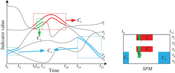
time intervals. Figure 1 shows an example to explain the Two-Dimensional (2D) spatio-temporal co-occurrence pattern, where the SPM has five regions and with a time duration [t
0, t
32]. In the right part of Figure 1,
 $P=\lcub C_{1}\comma \; C_{2}\comma \; C_{3}\rcub $
, and C
1 is a matrix including regions r
1, r
3 and time-slices t
9 − t
20. We know that the indicators (e.g. number of Voyages) of r
1 and r
3 are changing consistently in [t
9, t
20], shown in the left part of Figure 1 (dashed red rectangle).
Explanation of the spatio-temporal co-occurrence pattern (2D). Three matrices found here represent three different variation patterns of indicators. C 1, rows: r 1 and r 3, columns: [t 9, t 20]; C 2, rows: r 1, r 3 and r 4, columns: [t 10, t 12]; C 3, rows: r 4 and r 5, columns: [t 0, t 4] ∪ [t 24, t 32].

The problem could be extended to third or higher-order cases because AIS data are indexed by three or more variables. Without loss of generality, we use a third-order tensor to store data, in which T and Re are still dimensions. An extra dimension U is added to the matrix SPM, for instance, the ship type, formulating a spatio-temporal tensor
 $\underline{SPT}_{\Gamma \times L\times M}$
, whose (τ, l, m)-th element
 $\underline{SPT}\lpar \tau \comma \; l\comma \; m\rpar $
is the amount of Voyages (or leaving Trans and arriving Trans) in ship category u
l
in region r
m
during time interval
 $\lsqb t_{\tau - 1}\comma \; t_{\tau}\rsqb $
. Thus, the spatio-temporal co-occurrence pattern P discovered from
 $\underline{SPT}$
is a set of third-order data arrays
 $\lcub \underline{C}_{1}\comma \; \underline{C}_{2}\comma \; \cdots\comma \; \underline{C}_{K} \rcub $
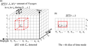
. An example illustrating the third-order problem definition is presented in Figure 2. Note that
 $\underline{C}_{k} \lpar \tau\comma \; l\comma \; m\rpar \ne \, \underline{SPT} \lpar \tau\comma \; l\comma \; m\rpar $
, while
 $\underline{C}_{k}$
holds some indices from
 $\underline{SPT}$
.
Explanation of the spatio-temporal co-occurrence pattern (3D). This example is to find groups of regions, time-slices and ship types (e.g. C k ), to discover whether the number of Voyages (the indicator) with certain ship types change similarly, both in certain regions and in certain time-slices.

Combining the second and higher-order cases to detect spatio-temporal co-occurrence pattern P, we define the following three criteria. Criterion 1 limits the scope of this paper, namely, we explore spatio-temporal knowledge from AIS data; criterion 2 shows that we focus on selecting indices of each dimension but not entries of SPM or
 $\underline{SPT}$
; criterion 3 shows consecutive variables must be partitioned into different categories.
-
(1) Data matrix SPM or tensor
 $\underline{SPT}$
must have T and Re dimensions.
-
(2) Indices of C k or
$\underline{C}_{k}$
are subsets from that of SPM or
$\underline{SPT}$
. -
(3) For third and higher-order tensors, extra dimensions (T and Re excluded) must be partitioned into different categories.


There are many combinations of variables to form data arrays, such as the region-speed matrix, time-width-speed tensor, and course-speed-ship type-length tensor. Of course, if we impose the above mentioned method on these data arrays, we can also find some relationships between different dimensions. However, exploring data arrays without T and Re dimensions is beyond the scope of this paper. For convenience, we use region-time matrix and region-time-ship type tensors as representatives in the following study.
2.2. Co-clustering Model
Approaches such as Principal Component Analysis (PCA), Non-negative Matrix Factorisation (NMF) and ordinary CP decomposition are alternatives for solving our problem. However, the results of PCA are too noisy to choose indices, and the new vectors produced are hard to explain. NMF also has noisy results, and its decomposition is non-unique. As to the ordinary CP decomposition, this is discussed in Equation (3) below.
Co-clustering selects rows and columns simultaneously in a matrix, while it groups along multiple modes in higher-order tensors. Various co-clustering formulations have been proposed. In this paper we use the version that imposes non-negativity and sparsity on the latent factors of matrix bilinear decomposition and tensor CP decomposition (Papalexakis et al., Reference Papalexakis, Sidiropoulos and Bro2013), by which co-clusters can be equivalently added one by one, in an additive way. Moreover, the selection of rows and columns becomes easy because of the reduction of noise.
Mathematically, the co-clustering scheme for matrices (non-negative sparse bilinear decomposition) can be stated as the minimisation of the following loss function:
 $$\mathop{\min}\limits_{A\ge {\rm {\bf 0}},B\ge {\rm {\bf 0}}} \vert \vert X-AB^T\vert \vert _F^2 +\lambda \sum\limits_{i,k} {\vert A(i,k)\vert } +\lambda \sum\limits_{j,k} {\vert B(j,k)\vert}$$
where X is the original I × J data matrix; A and B are factor matrices with size I × K and J × K respectively; K denotes the number of co-clusters extracted and λ is a sparsity controlling parameter. We rewrite the factor matrices with vectors and the problem can then be formulated as:
 $$\mathop{\min}\limits_{\{a_k \ge {\rm {\bf 0}},b_k \ge {\rm {\bf 0}}\}_{k=1}^K } \vert \vert X-\sum\limits_{k=1}^K {a_k b_k^T } \vert \vert _F^2 + \lambda \sum\limits_k {\vert \vert a_k \vert \vert _1 } +\lambda \sum\limits_k {\vert \vert b_k \vert \vert _1}$$
where
 $a_{k} b_{k}^{T} $
is a rank-1 matrix, and denotes a co-cluster, with some rows and columns made up of zeros. The ℓ1 norm part in Equation (2) is used as a sparsity enforcing surrogate to penalise the number of non-zero elements of a
k
and b
k
.
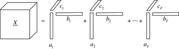
The co-clustering model is extended to third and higher-order cases. Here, we consider third-order tensors. Note that the CP decomposition factorises a tensor into a sum of component rank-1 tensors (as shown in Figure 3):
CP decomposition of a third-order tensor.

 $$\underline{X}\approx \sum\limits_{f=1}^F {a_f \circ b_f \circ c_f }$$
where
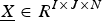 $\underline{X}\in R^{I\times J\times N}$
is the original data tensor, F is the number of components and the symbol “○” represents the vector outer product. However, a
f
, b
f
and c
f
are noisy here, so that it is hard to select the co-cluster from
 $a_{f} \circ b_{f} \circ c_{f} $
. Explanation of the components becomes difficult for the possible negative elements in the factors. Moreover, the uniqueness of ordinary CP decomposition is a problem. These problems can be solved by using the non-negative CP decomposition with sparse latent factors, which is formulated as follows:
 $$\mathop {\min}\limits_{\{a_k \ge {\rm {\bf 0}},b_k \ge {\bf{0}},c_k \ge {\bf{0}}\}_{k=1}^K } \vert \vert \underline{X}-\sum\limits_{k=1}^K {a_k \circ b_k \circ c_k \vert \vert _F^2 +\lambda \sum\limits_k {\vert \vert a_k \vert \vert _1 } +\lambda \sum\limits_k {\vert \vert b_k \vert \vert _1 } +\lambda \sum\limits_k {\vert \vert c_k \vert \vert _1}}$$
where K corresponds to the number of extracted co-clusters; a
k
, b
k
and c
k
are columns of factor matrices
 $A\in R^{I\times K}$
,
 $B\in R^{J\times K}$
and
 $C\in R^{N\times K}$
respectively;
 $a_{k} \circ b_{k} \circ c_{k}$
is an
 $I\times J\times N$
rank-1 third-order array, denoting a co-cluster, in which some rows, columns and fibres are made up of zeros. The function of the ℓ1 norm part in Equation (4) is as the same as that in Equation (2).
Papalexakis et al. (Reference Papalexakis, Sidiropoulos and Bro2013) discussed the impact of choice of λ and K. We use the higher-order co-clustering algorithm and its second-order analogue proposed by them to solve Equations (4) and (2).
3. DATA PROCESSING FRAMEWORK
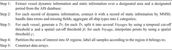
In real situations, raw AIS data are not expected to be utilised directly, but they must be processed into suitable forms. In this paper, we present a processing framework for AIS data, shown in Table 1. The details are as follows.
AIS data processing framework.

We extract vessel dynamic information and static information over a designated area and a designated period from a large AIS database. Available dynamic information contains MMSI (Maritime Mobile Service Identity), longitude, latitude, speed, status, course and UTC time (Coordinated Universal Time). The available static information contains MMSI, ship name, ship type, ship length, ship width and draught.
Next, we associate dynamic fields with static fields by MMSIs. However, data errors and missing fields are inevitable. Some records sharing a common MMSI have different ship name and ship type, and in this case we only keep the dynamic information. Data with erroneous MMSIs such as “1”, “6” and “99” are eliminated since a lot of vessels use these MMSIs. Some records have the same MMSI and ship name, but different ship type, length and width. We then consider two types of situations: can ship types can be aggregated or not? Illustrating that with an example, if the identifiers used to report ship type of these records are “70”, “72”, and “74”, then all these records will be classified as “cargo”; however, if the identifiers are “60”, “50” and “82”, corresponding to “passenger”, “pilot” and a type of “tanker” respectively, we only keep the dynamic fields. As a result, all ship types will be aggregated into L categories, coded from 1 to L.
Next is the trajectory processing. As basic spatio-temporal statistics from raw AIS data are not well suited to supporting the discovery and analysis of vessel movement patterns, the AIS data are processed into individual vessel trajectories according to MMSI. All the samples of the same MMSI over the entire period are chained together in increasing temporal order into a global trajectory. However, the global trajectory of a vessel may contain numerous stops and voyages. The global trajectory is then split into several Voyages, by using cut-off thresholds. If the time interval between two points of a Voyage is larger than α and during that interval the movement range is less than β, a stop occurs. The first point is deemed as the end of a Voyage and the second is deemed as the start of another. In addition, to deal with missing data, Linear interpolation is utilised to complement points of Voyages. For each Voyage, if the distance between two points is larger than γ, then
 $$Interpolation\_num = \displaystyle{{Missing\_dis}\over{Voyage\_dis}}\ast Voyage\_points\_num$$
where
 $Interpolation\_num$
and
 $Voyage\_points\_num$
denote the number of points needed to be interpolated and the number of points of the Voyage. While
 $missing\_dis$
and
 $Voyage\_dis$
stand for the distance need to be interpolated and the total distance of the Voyage. This interpolation ensures that each region a Voyage passes through can be detected. However, using Linear interpolation may cause some problems, which must be further studied. For instance, if there are “outlier” points, there will be a line interpolated between the correct and the outlier points, which may lead to some further errors in the analysis. Also, when a vessel sails around an island but there is a gap in the data, the interpolation may fix the points over a land area.
The next step is map segmentation and data mapping. The map of the concerned area is manually partitioned into M regions. Then we convert the map to a binary image. It is easy to recognise the borderlines since their pixels are in a colour that is not used to show the region pixels. Next is the Connected Component Labelling (CCL) step (Shapiro and Stockman, Reference Shapiro and Stockman2001), which finds individual regions by clustering non-borderline pixels. Finally, since each pixel has a region label and spatial coordinates, the AIS data mapped to these pixels can be given region labels.
Following these steps, we construct the SPM and
 $\underline{SPT}$
defined in Section 2.
4. EXPERIMENTAL RESULTS AND DISCUSSIONS
To verify the feasibility of our method and to discover knowledge about hidden connections among space, time, and vessel attributes, real case studies that include a second-order test and a third-order test were carried out. The calculation was processed in the MATLAB R2013b 64-bit program on a PC with Intel Core i7–4790 CPU at
 $3{\cdot}60\, \hbox{GHz}$
, 16-GB RAM equipped with Windows 7.
4.1. Dataset and Data Processing Results
We utilised a real-world AIS dataset with respect to Shanghai port, with data from military vessels removed. Table 2 shows details of the AIS data samples after eliminating data with erroneous MMSIs.
Details of AIS data samples.

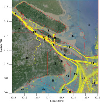
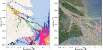
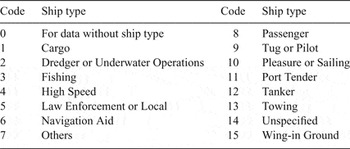
Ship types were divided into 15 categories, as listed in Table 3. After processing, 4,868 ships in the dataset had ship types, and the type numbers of the rest were set to 0. The temporal cut-off threshold α and spatial cut-off threshold β for trajectory splitting were set to 5 hours and 50 kilometres respectively, and the Linear interpolation threshold γ was also set to 50 kilometres. After trajectory processing, we obtained 12,011 different Voyages and 1,208,109 data records. Moreover, the map was segmented into 32 regions and time duration was partitioned into 72 slices, meaning each lasted for 2 hours. Figures 4 and 5 show the results of data processing.
The AIS samples and the result of map segmentation.

The samples with region labels (left) and the Voyages after trajectory processing (right).

Ship category taxonomy.

4.2. Second-order Case
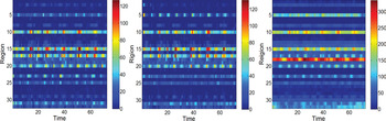
The statistical results of the region-time matrices are shown in Figure 6. The amount of leaving Trans, arriving Trans, and total Voyages in each region in each time interval were counted respectively. When checking these original matrices, we can see some regions have large flows while others have little. However, it is difficult to find useful patterns intuitively because the data are noisy.
The region-time matrices. Left: the leaving SPM. Middle: the arriving SPM. Right: the Voyages SPM. Different value of entry in a matrix is represented by a different colour.

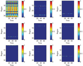
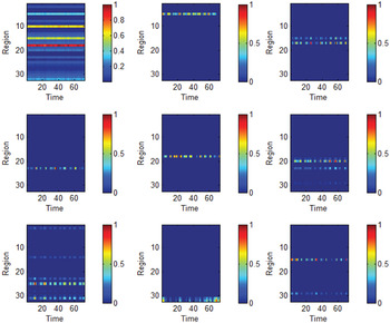
We use the leaving SPM and the Voyages SPM as examples. Co-clusters extracted from these SPMs are illustrated in Figures 7 and 8. The co-clusters can be fitted in an additive way, and the result is not sensitive to the parameter K in Equation (2), so we extracted the first nine co-clusters in this paper. The parameter λ is self-adaptive in the second-order algorithm. Moreover, to discover some possible patterns on the time mode, we normalised the rows of the leaving SPM before calculation. By doing this, the variation of values through the time mode can be captured. Similarly, the columns in the Voyages SPM were normalised to find possible patterns in the region mode. The value of each entry in a co-cluster reflects the proportion of leaving Trans or Voyages that was assigned to this co-cluster, which can also be explained as “the degree of belonging” to this co-cluster, and was scaled to 0-1 for each co-cluster to show more clearly in pictures.
Co-clusters 1-9 extracted from the leaving SPM by normalisation of the time mode.

Co-clusters 1-9 extracted from the VoyagesSPM by normalisation of the region mode.

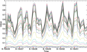
In Figure 7, co-cluster 1 contains most regions and time-slices, reflecting that the leaving behaviour of vessels in most of regions in the area of interest share a common type of time rule, while co-clusters 2–9 represent other time regularities. Comparing co-cluster 1 in Figure 7 with the original leaving SPM in Figure 6, we find that in co-cluster 1 noise is reduced and data are fluctuating periodically along the rows. Values of co-cluster 1 are then depicted in Figure 9, in which the numbers on the horizontal axis are transferred to Shanghai local time (Beijing time, 8 hours earlier than UTC time). We can see approximately six peaks from 0800 on 26 October to 0800 on 1 November, each peak appears at about
 $1000 \sim 1400$
while valleys appear at about
 $0200 \sim 0600$
. Note that this periodic pattern cannot be found directly from the original matrix.
Co-cluster 1 extracted from the leaving SPM, showing a periodic pattern on the time mode. Time-slices were transferred to intervals of local time, and each line stands for a region.

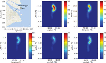
Next, we validated the discovered periodic pattern in Figure 9 using kernel density estimation. The density maps of region 18 over a one day period are illustrated in Figure 10, showing that the vessel volume changes along with time and this phenomenon accords with people's daily lives.
Density maps of region 18. Left up: the region validated. Middle up: h10-12, d29. Right up: h16-18, d29. Left down: from h22 to midnight, d29. Middle down: h2-4, d30. Right down: h6-8 d30.

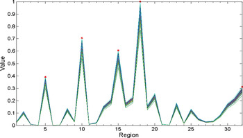
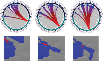
In Figure 8, each co-cluster captures a fluctuation pattern on the region dimension for each time-slice. Here, we also interpret the pattern of co-cluster 1 as it contains the majority of regions and time-slices. Values of co-cluster 1 extracted from the Voyages SPM are illustrated in Figure 11. We can clearly see that in almost all time-slices, the values of each region contained by this co-cluster maintain a steady level. This reflects the fact that the proportions of Voyages of many regions in the area of interest do not change much by time. Regions that have large flows always have large flows, and regions with small flows always stay at a low flow level. In addition, we see regions 5, 10, 15, 18 and 32 have a relatively larger proportion of Voyages, which are all main channels on the map. Figure 12 depicts flows derived from regions 5, 10 and 15, showing that flows always transit along main channels. For instance, large flows derived from region 10 reach to regions 5, 8, 15 and 18, with the former three located in the main channels of the Yangtze River, and the latter located in the Huangpu River, which crosses downtown Shanghai. However, only very small flows reach to other regions.
Co-cluster 1 extracted from the Voyages SPM. Each line stands for a time-slice, and in almost all time-slices, the values of each region contained by this co-cluster maintains a steady level.

Flows from origins to destinations (red: origins; blue: destinations). Origins: region 5 (left), region 10 (middle), region 15 (right).

Compared with co-cluster 1, the other co-clusters in Figure 8 have regions whose values change by time. For example, co-cluster 8 in Figure 8 contains region 31, 32 and some time-slices, in which the values of these two regions change by time in a coordinated way. The reason found for this coordination was that they are neighbours located in the southeast of the map. Note that regions 31 and 32 are also included in co-cluster 1, an interpretation of this is that co-cluster 1 captures the non-varying part of values while co-cluster 8 captures the variation shared by only regions 31 and 32.
4.3. Third-order Case
By normalisation of the ship type dimension before calculation, each co-cluster extracted from the ship type-region-time tensor denotes a pattern that shows the distribution change of Voyages on the ship type mode (i.e. vessels with certain ship types exist in particular regions in particular time-slices). Like the second-order case, the value of each entry in a co-cluster reflects the proportion of Voyages that was assigned to this co-cluster, or its “degree of belonging” to this co-cluster.
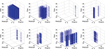
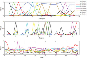
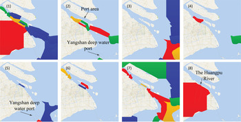
Figure 13 shows co-clusters 1 to 8 extracted from the ship type-region-time tensor, and Figure 14 presents the value of co-clusters on three modes, ship type, region and time. From the ship type mode on the top panel in Figure 14, we see that all ship types in co-cluster 1 (blue line) have values lager than 0·2 (the significant threshold for ship types), meaning that this co-cluster includes all ship types. However, values of ship types in other co-clusters show more complex modes than that for co-cluster 1. Each co-cluster of 2 to 8 contains one or more ship types, nearly all of which are different from one co-cluster to another (without considering values less than 0·2). As to the region mode in Figure 14, we see some regions, which have larger flows (e.g. region 5, 10, 15, 20), that are shared by different co-clusters. In addition, all co-clusters are approximately continuous on the time mode, see Figure 13. The values are approximately constant, denoting that time impact on these co-clusters is not noteworthy. Detailed interpretations about these eight co-clusters are given below.
Co-clusters 1-8 extracted from the ship type-region-time tensor by normalisation of the ship type mode. The indicator used to fill the entries of original tensor is the number of Voyages.

Each mode of the decomposition of ship type-region-time tensor, with all 8 co-clusters plotted overlying each other.

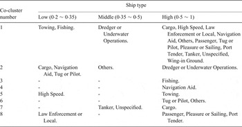
Ship types of each co-cluster extracted from the ship type-region-time tensor are described in Table 4. Regions of each co-cluster are shown on the maps in Figure 15, and the significant threshold for regions is 0·1. Since the time dimension has little influence on these co-clusters, we ignore it. By analysing regions and ship types of each co-cluster, we can conclude the meaning hidden in each co-cluster as follows:
-
• Co-cluster 1: main channels. This co-cluster contains all ship types, and all regions in it have heavy traffic, especially those located in the Yangtze and Huangpu Rivers.
-
• Co-cluster 2: port and entrance areas. Dredgers or underwater operation vessels mainly exist in port areas and port entrances, to ensure large ships from the sea can enter the port. Some tankers and navigation aids are also distributed in these areas.
-
• Co-cluster 3: fishing zone. Only fishing vessels are included in this co-cluster, and regions here are all far away from land.
-
• Co-cluster 4: areas with navigation aids. Navigation aids included by this co-cluster mainly exist in region 10, which is a busy inner water port area.
-
• Co-cluster 5: deep water port. Yanghshan deep water port is in region 30, connecting to downtown Shanghai with a channel. It is to be expected that there are many towing ships.
-
• Co-cluster 6: inner water ports. Tugs and pilot vessels are mainly contained by this co-cluster, because all regions in this co-cluster have inner water ports.
-
• Co-cluster 7: active areas of cargo ships and tankers. In this co-cluster, areas which cargo ships and tankers move across have a large range, from inner water to the open sea.
-
• Co-cluster 8: entertainment area. The Huangpu River in Shanghai is a famous tourist attraction, each day many cruise ships and passenger ships sail back and forth along it. Since it is so busy, some port tenders, law enforcement vessels and local vessels are also distributed in this region.
Regions of each co-cluster extracted from the ship type-region-time tensor. The values on the region mode are coloured red (0·5~ 1), yellow (0·35~ 0·5), green (0·2~ 0·35) and blue (0·1~ 0·2).

Ship types of each co-cluster extracted from the ship type-region-time tensor. The values on ship type mode are grouped to low, middle, and high levels.

5. CONCLUSION
Transforming massive amounts of AIS raw data into high-level knowledge is of great importance to maritime situational awareness applications. In this paper, we proposed a vessel spatio-temporal co-occurrence pattern to unveil vessel spatio-temporal knowledge and utilised the co-clustering method to detect this from AIS trajectories. Some definitions related to vessel trajectory and a suite of data processing methods were introduced in this work. The vessel spatio-temporal co-occurrence pattern provides insight into not only a single dimension (e.g. the relation between regions), but also relationships among multiple dimensions. Experimental results show that we discovered patterns in time and space modes from real AIS trajectories, as well as the function of regions. We found and validated groups of regions and time-slices (or more than these two dimensions) that consistently behave in a coordinated way, suggesting the existence of connections among these dimensions.
Future work may include exploring the impact of choice of thresholds α, β and γ for trajectory processing, exploring the construction of data arrays to find fleet activity patterns, extending the time span to find long term patterns (e.g. weekly, monthly, and quarterly), expanding the area of interest to find long-range patterns, and finding patterns from cross-domain data sources.
ACKNOWLEDGMENTS
This work was supported by the National Natural Science Foundation of China (Grants No. 71571186 and 71471176).