1 Introduction
The Monin–Obukhov similarity theory (MOST) (Obukhov Reference Obukhov1946; Monin & Obukhov Reference Monin and Obukhov1954) is the theoretical foundation for understanding the surface layer of the atmospheric boundary layer. It hypothesizes that all surface-layer statistics, when scaled using the surface-layer parameters, depend only on the non-dimensional parameter
 $z/L$
, where
 $L=-u_{\ast }^{3}/(\unicode[STIX]{x1D705}(g/\unicode[STIX]{x1D6E9})Q)$
, with
 $z$
,
 $L$
,
 $u_{\ast }$
,
 $\unicode[STIX]{x1D705}$
,
 $g$
,
 $\unicode[STIX]{x1D6E9}$
and
 $Q$
the distance from the surface, the Obukhov length, the friction velocity, the von Kármán constant, the gravity acceleration, the mean potential temperature and the surface temperature flux, respectively. Many important surface-layer statistics have been found to follow MOST, e.g. the non-dimensional mean shear and potential temperature gradients, turbulent kinetic energy budget, the vertical velocity variance, and the inertial-range spectrum and cospectrum (e.g. Businger et al.
Reference Businger, Wyngaard, Izumi and Bradley1971; Wyngaard & Coté Reference Wyngaard and Coté1971; Wyngaard, Coté & Izumi Reference Wyngaard, Coté and Izumi1971; Kaimal et al.
Reference Kaimal, Wyngaard, Izumi and Coté1972; Kaimal Reference Kaimal1978). However, it has also been known since the late 1950s that a number of important surface-layer statistics, such as the horizontal velocity variances and the large-scale horizontal velocity spectra, do not conform to MOST (e.g. Lumley & Panofsky Reference Lumley and Panofsky1964; Kaimal et al.
Reference Kaimal, Wyngaard, Izumi and Coté1972; Kaimal Reference Kaimal1978; Caughey & Palmer Reference Caughey and Palmer1979), rendering the surface-layer similarity in the MOST framework incomplete and raising questions about the existence of general similarity in the surface layer. The non-MOST behaviour also suggests that some fundamental physics is missing from our understanding of the surface layer. In spite of many previous efforts to address this issue (e.g. Betchov & Yaglom Reference Betchov and Yaglom1971; Zilitinkevich Reference Zilitinkevich1971; Kader Reference Kader1988; Yaglom Reference Yaglom1994), a resolution has proven to be challenging.
To understand the origin of the incomplete similarity in the MOST framework, Tong & Nguyen (Reference Tong and Nguyen2015) examined the assumptions in MOST: (1)
 $z$
represents the length scale of the energy-containing eddies, and (2)
 $L$
is the characteristic vertical length scale, ‘the height of the sub-layer of dynamic turbulence’ (Obukhov Reference Obukhov1946). Regarding assumption (1), for turbulence statistics in a near-neutral surface layer and for certain statistics in a convective surface layer (e.g. the vertical velocity variance), the energy-containing length scale is of the order of
 $z$
, which therefore is the appropriate length scale in MOST. In a convective surface layer, however, the energy-containing scales for some important statistics (e.g. horizontal velocity variances) are not
 $z$
(in fact, the scales of the convective eddies at a height
 $z$
range from
 $z$
to
 $z_{i}$
), and therefore are not properly represented in MOST, where
 $z_{i}$
is the boundary layer (inversion) height. Consequently, the parameter
 $z/L$
does not characterize the relative influence of buoyancy and shear effects, and MOST does not provide the correct scaling for these statistics.
Since the use of
 $z$
as the eddy length scale in the similarity theory is not always justified, addressing the issue of incomplete similarity requires that the scales of turbulent eddies be explicitly included in the similarity theory. To achieve this goal, multi-point statistics, which are functions of the separations between points, thereby explicitly containing the scale information, need to be used. Consequently, a general similarity theory should be formulated in terms of multi-point statistics (Tong & Nguyen Reference Tong and Nguyen2015).
To form the similarity variables for multi-point statistics, which in general contain both horizontal and vertical separations between the points, a horizontal characteristic length scale is needed (
 $L$
is the characteristic vertical length scale in MOST). The geometry of the boundary layer, which is horizontally homogeneous, does not impose one. Tong & Nguyen (Reference Tong and Nguyen2015) pointed out that the new physical understanding gained in their AHATS field programme (Nguyen et al.
Reference Nguyen, Horst, Oncley and Tong2013; Nguyen & Tong Reference Nguyen and Tong2015) provides this length scale. The results of the investigations on the turbulent (subgrid-scale) stress budget in the convective surface layer (Nguyen et al.
Reference Nguyen, Horst, Oncley and Tong2013; Nguyen & Tong Reference Nguyen and Tong2015; Tong & Nguyen Reference Tong and Nguyen2015) suggest that fluctuations of wavenumber
 $k$
at the height
 $z\sim 1/k$
, where the buoyant production occurs, are coupled to those of
 $k$
at
 $z\ll 1/k$
, where the production is small, by the convective eddies through the pressure transport and the pressure–strain-rate correlation; therefore the dynamics of these motions are influenced by shear and buoyancy productions in a similar way. Thus the new physics suggests that the Obukhov length is not only the characteristic vertical length scale in surface-layer similarity, as hypothesized in MOST, but also the characteristic horizontal length scale (for
 $1/z_{i}\ll k\ll 1/z$
), and that
 $-kL$
is another non-dimensional parameter for the surface-layer similarity (in addition to
 $z/L$
).
Based on the above considerations, a generalized surface-layer similarity hypothesis, the multi-point Monin–Obukhov similarity (MMO), was recently proposed (Tong & Nguyen Reference Tong and Nguyen2015). It hypothesizes that: (1) complete similarity exists in the surface layer, but it can only be represented by multi-point statistics; and (2) the Obukhov length is the characteristic length scale in both horizontal and vertical directions within MMO. Therefore, all multi-point statistics, non-dimensionalized using the surface-layer parameters, depend only on the reference height and separations non-dimensionalized using
 $L$
.
MMO was formulated in terms of the joint probability density function of velocity differences, hypothesizing that all multi-point velocity difference statistics have similarity properties (Tong & Nguyen Reference Tong and Nguyen2015). Therefore the surface-layer similarity is complete in the MMO framework, i.e. the similarity properties as hypothesized by MMO are valid for all multi-point velocity and (transported) scalar statistics. MMO has been successfully employed to predict turbulence spectra (Tong & Nguyen Reference Tong and Nguyen2015).
With the establishment of MMO, the similarity properties of one-point statistics can be derived from their relationships with multi-point statistics. For example, the scale of the dominant contribution to a velocity variance can be obtained using its spectrum. If this scale is a surface-layer scale, the variance follows MOST (e.g. the vertical velocity variance). Otherwise it does not (e.g. the horizontal velocity variances). Therefore, MOST can be regarded as a special case of MMO.
Similar to MOST, MMO is also proposed as hypotheses, however. Measurements can only provide support to it, but cannot positively prove it. In the present study, we use first principles to derive it. Starting from the Navier–Stokes equations and the potential temperature equation, we employ the method of matched asymptotic expansions to derive analytically the MMO similarity properties for the two-dimensional horizontal Fourier transforms of the velocity and potential temperature in a convective surface layer, which are equivalent to the two-point velocity and temperature differences. We show that
 $L$
is indeed a characteristic horizontal length scale in the convective surface layer and that the Fourier transforms conform to the MMO scaling. Note that, although we only derive the scaling properties of the two-point statistics,
 $L$
as a length scale in both horizontal and vertical directions can be used to scale other multi-point statistics, thereby providing strong analytical support to MMO.
The method of matched asymptotic expansions (Van Dyke Reference Van Dyke1975; Bender & Orszag Reference Bender and Orszag1978; Cousteix & Mauss Reference Cousteix and Mauss2007) has been previously employed to derive Kolmogorov’s hypotheses by Lundgren (Reference Lundgren2003) who used two-point velocity differences, which are easier to handle mathematically than Fourier transforms, especially the nonlinear terms in the Navier–Stokes and temperature equations. We choose to analyse the Fourier transforms because the differences for the vertical velocity might not have power-law scaling. For a horizontally homogeneous velocity field,
 $u_{i}$
, we define its horizontal Fourier transform over a horizontal physical domain of size
 ${\mathcal{L}}\times {\mathcal{L}}$
:
 $$\begin{eqnarray}\displaystyle \hat{u} _{i}(\boldsymbol{k})=\frac{1}{{\mathcal{L}}^{2}}\int _{0}^{{\mathcal{L}}}u_{i}(\boldsymbol{x},t)\text{e}^{-\text{i}\boldsymbol{k}\boldsymbol{x}}\,\text{d}\boldsymbol{x}, & & \displaystyle\end{eqnarray}$$
where
 $\boldsymbol{k}$
is the horizontal wavenumber vector. Dividing the usual definition of the transform by
 ${\mathcal{L}}^{2}$
gives the Fourier transform the same dimension as well as the same scaling properties as the velocity, which is convenient for the scaling analysis. The Fourier transform of the potential temperature
 $\hat{\unicode[STIX]{x1D703}}$
is defined similarly.
The transport equations of the Fourier components of the velocity and potential temperature, obtained from the Navier–Stokes equations and the potential temperature equation, are:
 $$\begin{eqnarray}\displaystyle & & \displaystyle \frac{\unicode[STIX]{x2202}\hat{u} _{j}(\boldsymbol{k},t)}{\unicode[STIX]{x2202}t}+{\mathcal{L}}^{2}\int \hat{u} _{3}(\boldsymbol{k}^{\prime })\frac{\unicode[STIX]{x2202}\hat{u} _{j}(\boldsymbol{k}-\boldsymbol{k}^{\prime })}{\unicode[STIX]{x2202}x_{3}}\,\text{d}\boldsymbol{k}^{\prime }+{\mathcal{L}}^{2}\int \text{i}k_{m}^{\prime }\hat{u} _{j}(\boldsymbol{k}^{\prime })\hat{u} _{m}(\boldsymbol{k}-\boldsymbol{k}^{\prime })\,\text{d}\boldsymbol{k}^{\prime }\nonumber\\ \displaystyle & & \displaystyle \quad =-\text{i}k_{j}\hat{p}-2\unicode[STIX]{x1D716}_{jnl}\unicode[STIX]{x1D6FA}_{n}\hat{u_{l}}(\boldsymbol{k})+\unicode[STIX]{x1D708}\frac{\unicode[STIX]{x2202}^{2}\hat{u} _{j}}{\unicode[STIX]{x2202}x_{3}^{2}}-\unicode[STIX]{x1D708}k^{2}\hat{u} _{j}(\boldsymbol{k}),\quad j=1,2,~m=1,2,\end{eqnarray}$$
 $$\begin{eqnarray}\displaystyle & & \displaystyle \frac{\unicode[STIX]{x2202}\hat{u} _{3}(\boldsymbol{k},t)}{\unicode[STIX]{x2202}t}+{\mathcal{L}}^{2}\int \hat{u} _{3}(\boldsymbol{k}^{\prime })\frac{\unicode[STIX]{x2202}\hat{u} _{3}(\boldsymbol{k}-\boldsymbol{k}^{\prime })}{\unicode[STIX]{x2202}x_{3}}\,\text{d}\boldsymbol{k}^{\prime }+{\mathcal{L}}^{2}\int \text{i}k_{m}^{\prime }\hat{u} _{3}(\boldsymbol{k}^{\prime })\hat{u} _{m}(\boldsymbol{k}-\boldsymbol{k}^{\prime })\,\text{d}\boldsymbol{k}^{\prime }\nonumber\\ \displaystyle & & \displaystyle \quad =-\frac{\unicode[STIX]{x2202}\hat{p}}{\unicode[STIX]{x2202}x_{3}}-2\unicode[STIX]{x1D716}_{jnl}\unicode[STIX]{x1D6FA}_{n}\hat{u_{l}}(\boldsymbol{k})+\unicode[STIX]{x1D708}\frac{\unicode[STIX]{x2202}^{2}\hat{u} _{3}}{\unicode[STIX]{x2202}x_{3}^{2}}-\unicode[STIX]{x1D708}k^{2}\hat{u} _{3}(\boldsymbol{k})+\frac{g}{\unicode[STIX]{x1D6E9}}\hat{\unicode[STIX]{x1D703}},\quad j=3,~m=1,2,\end{eqnarray}$$
 $$\begin{eqnarray}\displaystyle & & \displaystyle \frac{\unicode[STIX]{x2202}\hat{\unicode[STIX]{x1D703}}(\boldsymbol{k},t)}{\unicode[STIX]{x2202}t}+{\mathcal{L}}^{2}\int \hat{u} _{3}(\boldsymbol{k}^{\prime })\frac{\unicode[STIX]{x2202}\hat{\unicode[STIX]{x1D703}}(\boldsymbol{k}-\boldsymbol{k}^{\prime })}{\unicode[STIX]{x2202}x_{3}}\,\text{d}\boldsymbol{k}^{\prime }+{\mathcal{L}}^{2}\int \text{i}k_{m}^{\prime }\hat{\unicode[STIX]{x1D703}}(\boldsymbol{k}^{\prime })\hat{u} _{m}(\boldsymbol{k}-\boldsymbol{k}^{\prime })\,\text{d}\boldsymbol{k}^{\prime }\nonumber\\ \displaystyle & & \displaystyle \quad =D\frac{\unicode[STIX]{x2202}^{2}\hat{\unicode[STIX]{x1D703}}}{\unicode[STIX]{x2202}x_{3}^{2}}-Dk^{2}\hat{\unicode[STIX]{x1D703}}(\boldsymbol{k}),\quad m=1,2,\end{eqnarray}$$
where
 $\unicode[STIX]{x1D708}$
,
 $D$
,
 $\unicode[STIX]{x1D6FA}$
and
 $\unicode[STIX]{x1D716}_{jnl}$
are the kinematic viscosity, the thermal diffusivity, the Earth’s rotation vector and the alternating symbol, respectively. Since the viscous and diffusion terms are only relevant to the inertial and dissipation-scale fluctuations (Kolmogorov turbulence), we omit them in the equations hereafter. In the rest of the paper we first identify the structure of the surface layer, showing that it has a boundary layer structure in the horizontal wavenumber space, and therefore can be analysed as a singular perturbation problem. We then perform the method of matched asymptotic expansions of equations (1.2), (1.3) and (1.4). We show that
 $L$
is the horizontal characteristic length scale and that the Fourier transforms are functions of the non-dimensional wavenumber
 $-kL$
, proving the MMO hypotheses for two-point horizontal separation, and thereby providing strong support to MMO for general multi-point statistics.
We then determine the coefficients in the expansions using the velocity spectra obtained using large-eddy simulation (LES) and compare the composite expansions with the LES spectra. We choose to use LES rather than measurements for two reasons. First, the spectra given by the asymptotic expansions are two-dimensional spectra and ring-integrated spectra, both depending on the magnitude of the horizontal wavenumber. For a ring-integrated spectrum with a scaling range less steep than
 $-1$
, i.e. the exponent greater than
 $-1$
(e.g. the vertical velocity spectrum for
 $k<1/z$
), its one-dimensional counterpart does not have the same scaling exponent (a one-dimensional spectrum for a horizontally isotropic field cannot have a positive scaling exponent). To compare such a spectrum with measurements, the two-dimensional spectrum must be measured. Therefore, MMO presents a challenge to measurement techniques. In addition, for the streamwise velocity spectrum, to make proper comparisons with measurements, it is important that the two scaling ranges are evident, i.e. sufficiently wide (greater than a decade). Such comparisons would probably require new measurements, which therefore is a project by itself and is deferred to future work.
The LES code, presented in detail in Moeng (Reference Moeng1984), has been well documented in the literature (Moeng & Wyngaard Reference Moeng and Wyngaard1988; Sullivan, McWilliams & Moeng Reference Sullivan, McWilliams and Moeng1994, Reference Sullivan, Mcwilliams and Moeng1996), and has been later refined by Otte & Wyngaard (Reference Otte and Wyngaard2001). We simulate three cases of atmospheric boundary layer (ABL) flow: (1) a weakly unstable and (2) a moderately unstable ABL driven by a combination of geostrophic winds and surface heating, and (3) a nearly free convective ABL driven by a constant surface heat flux and weak geostrophic winds. The subgrid-scale (SGS) fluxes are parametrized using the Kosović model (Kosović Reference Kosović1997). The simulations are implemented on a mesh of
 $1024^{3}$
and
 $2048^{3}$
grid points (only
 $1024^{3}$
for weakly unstable case), with a domain size of
 $5120~\text{m}\times 5120~\text{m}$
in the horizontal and
 $2048~\text{m}$
in the vertical. Tong & Nguyen (Reference Tong and Nguyen2015) have demonstrated that the scaling of the spectra is not sensitive to the SGS model employed, although the magnitude might depend on the model.
2 The structure of the surface layer
In this section we examine the structure of the surface layer and identify the mathematical (singular perturbation) problem. We define a set of non-dimensional (convective) variables as follows:
 $$\begin{eqnarray}\displaystyle \left.\begin{array}{@{}c@{}}\displaystyle \hat{u} _{1}=w_{\ast }\hat{u} _{1c},\quad \hat{u} _{3}=w_{\ast }\hat{u} _{3c},\quad t=\frac{z_{i}}{w_{\ast }}\unicode[STIX]{x1D70F},\\ \displaystyle {\mathcal{L}}=z_{i}{\mathcal{L}}_{c},\quad \boldsymbol{k}=\frac{1}{z_{i}}\boldsymbol{k}_{c},\quad x_{3}=z_{i}x_{3c},\quad \hat{p}=w_{\ast }^{2}\hat{p}_{c},\\ \displaystyle \hat{\unicode[STIX]{x1D703}}=\frac{Q}{w_{\ast }}\hat{\unicode[STIX]{x1D703}}_{c},\quad \frac{\unicode[STIX]{x2202}\hat{p}}{\unicode[STIX]{x2202}x_{3}}=\frac{w_{\ast }^{2}}{z_{i}}\left(\frac{\unicode[STIX]{x2202}\hat{p}}{\unicode[STIX]{x2202}x_{3}}\right)_{c},\\ \displaystyle \frac{\unicode[STIX]{x2202}U}{\unicode[STIX]{x2202}x_{3}}=\frac{u^{\prime \prime }}{z_{i}}\left(\frac{\unicode[STIX]{x2202}U}{\unicode[STIX]{x2202}x_{3}}\right)_{c},\quad \frac{\unicode[STIX]{x2202}\unicode[STIX]{x1D6E9}}{\unicode[STIX]{x2202}x_{3}}=\frac{Q}{w^{\prime }z_{i}}\left(\frac{\unicode[STIX]{x2202}\unicode[STIX]{x1D6E9}}{\unicode[STIX]{x2202}x_{3}}\right)_{c}.\end{array}\right\} & & \displaystyle\end{eqnarray}$$
Here
 $w_{\ast }=(gQz_{i}/\unicode[STIX]{x1D6E9}_{0})^{1/3}$
,
 $Q$
,
 $U$
and
 $\unicode[STIX]{x1D6E9}$
are the mixed-layer (Deardorff) velocity scale, the surface potential temperature flux, the mean streamwise velocity and the mean potential temperature, respectively, and
 $u^{\prime \prime }$
and
 $Q/w^{\prime }$
are the velocity and temperature scales for
 $\unicode[STIX]{x2202}U/\unicode[STIX]{x2202}x_{3}$
and
 $\unicode[STIX]{x2202}\unicode[STIX]{x1D6E9}/\unicode[STIX]{x2202}x_{3}$
, respectively, which will be determined later in this paper. The direction of the mean velocity is defined as the
 $x_{1}$
direction. The equation for
 $\hat{u} _{1c}$
is
 $$\begin{eqnarray}\displaystyle & & \displaystyle \frac{\bar{\text{D}}\hat{u} _{1c}}{\text{D}\unicode[STIX]{x1D70F}}\frac{w_{\ast }^{2}}{z_{i}}+z_{i}^{2}{\mathcal{L}}_{c}^{2}\int \hat{u} _{3c}\frac{\unicode[STIX]{x2202}\hat{u} _{1c}}{\unicode[STIX]{x2202}x_{3c}}\,\text{d}\boldsymbol{k}_{c}^{\prime }\,\frac{w_{\ast }^{2}}{z_{i}}\frac{1}{z_{i}^{2}}+\hat{u} _{3c}\left(\frac{\unicode[STIX]{x2202}U}{\unicode[STIX]{x2202}x_{3}}\right)_{c}w_{\ast }\frac{u^{\prime \prime }}{z_{i}}+z_{i}^{2}{\mathcal{L}}_{c}^{2}\int \hat{u} _{1c}\text{i}k_{1c}^{\prime }\hat{u} _{1c}\,\text{d}\boldsymbol{k}_{c}^{\prime }\,\frac{w_{\ast }^{2}}{z_{i}}\frac{1}{z_{i}^{2}}\nonumber\\ \displaystyle & & \displaystyle \quad =-\text{i}k_{1c}\hat{p}_{c}\frac{w_{\ast }^{2}}{z_{i}}-2\unicode[STIX]{x1D716}_{1nl}\unicode[STIX]{x1D6FA}_{n}\hat{u_{l}}(\boldsymbol{k}).\end{eqnarray}$$
The Coriolis term, which scales as
 $fw_{\ast }$
, where
 $f=2\unicode[STIX]{x1D6FA}_{3}$
is the Coriolis parameter, is typically an order of magnitude smaller than the dominant (e.g. time-derivative) terms, and therefore is neglected. The horizontal derivative of the horizontal velocity scales differently than the vertical derivative at the large scales, and these are written as different terms hereafter.
Dividing (2.2) by
 $w_{\ast }^{2}/z_{i}$
results in
 $$\begin{eqnarray}\displaystyle \left.\begin{array}{@{}c@{}}\displaystyle \frac{\bar{\text{D}}\hat{u} _{1c}}{\text{D}\unicode[STIX]{x1D70F}}+{\mathcal{L}}_{c}^{2}\int \hat{u} _{3c}\frac{\unicode[STIX]{x2202}\hat{u} _{1c}}{\unicode[STIX]{x2202}x_{3c}}\,\text{d}\boldsymbol{k}_{c}^{\prime }+\unicode[STIX]{x1D716}\hat{u} _{3c}\left(\frac{\unicode[STIX]{x2202}U}{\unicode[STIX]{x2202}x_{3}}\right)_{c}+{\mathcal{L}}_{c}^{2}\int \hat{u} _{1c}\text{i}k_{1c}^{\prime }\hat{u} _{1c}\,\text{d}\boldsymbol{k}_{c}^{\prime }=-\text{i}k_{1c}\hat{p_{c}}.\\ \displaystyle \text{TD}\hspace{51.21504pt}\text{CS}\hspace{62.59596pt}\text{S}\hspace{79.6678pt}\text{N1}\hspace{62.59596pt}\text{P}\end{array}\right\} & & \displaystyle\end{eqnarray}$$
The time-derivative and mean advection (
 $-U\text{i}k\hat{u} _{1}$
) terms have been combined into a mean substantial derivative (TD) so that the time rate of change reflects the turbulence time scale rather than the mean advection time scale. The second term on the left-hand side (LHS) represents convection-induced stress (CS), and is negligible above the convection-induced-stress layer (Businger Reference Businger1973; Sykes, Henn & Lewellen Reference Sykes, Henn and Lewellen1993; Grachev, Fairall & Zilitinkevich Reference Grachev, Fairall and Zilitinkevich1997; Zilitinkevich et al.
Reference Zilitinkevich, Hunt, Esau, Grachev, Lalas, Akylas, Tombrou, Fairall, Fernando, Baklanov and Joffre2006). The last (nonlinear) term (N1) on the LHS and the pressure-gradient term (P) are the leading terms, balancing each other. The former scales as
 $w_{\ast }^{2}/z_{i}$
; therefore, the latter must be of the same order of magnitude. There is a small parameter in the term containing the mean shear (S) in equation (2.3),
 $$\begin{eqnarray}\displaystyle \unicode[STIX]{x1D716}=\frac{u^{\prime \prime }}{w_{\ast }}, & & \displaystyle\end{eqnarray}$$
where
 $u^{\prime \prime }$
will be shown to be
 $u_{\ast }$
in § 3 (3.11). In the surface layer
 $\hat{u} _{3c}\ll 1$
. However,
 $\hat{u} _{3c}(\unicode[STIX]{x2202}U/\unicode[STIX]{x2202}x_{3})_{c}$
is of order one since
 $\unicode[STIX]{x2202}U/\unicode[STIX]{x2202}x_{3}\sim u^{\prime \prime }/z$
.
The equation for
 $\hat{u} _{3c}$
is
 $$\begin{eqnarray}\displaystyle & & \displaystyle \frac{\bar{\text{D}}\hat{u} _{3c}}{\text{D}\unicode[STIX]{x1D70F}}\frac{w_{\ast }^{2}}{z_{i}}+z_{i}^{2}{\mathcal{L}}_{c}^{2}\int \hat{u} _{3c}\frac{\unicode[STIX]{x2202}\hat{u} _{3c}}{\unicode[STIX]{x2202}x_{3c}}\,\text{d}\boldsymbol{k}_{c}^{\prime }\,\frac{w_{\ast }^{2}}{z_{i}}\frac{1}{z_{i}^{2}}+z_{i}^{2}{\mathcal{L}}_{c}^{2}\int \hat{u} _{1c}\text{i}k_{1c}^{\prime }\hat{u} _{3c}\,\text{d}\boldsymbol{k}_{c}^{\prime }\,\frac{w_{\ast }^{2}}{z_{i}}\frac{1}{z_{i}^{2}}\nonumber\\ \displaystyle & & \displaystyle \quad =-\left(\frac{\unicode[STIX]{x2202}\hat{p}}{\unicode[STIX]{x2202}x_{3}}\right)_{c}\frac{w_{\ast }^{2}}{z_{i}}+\frac{g}{\unicode[STIX]{x1D6E9}}\frac{Q}{w_{\ast }}\hat{\unicode[STIX]{x1D703}}_{c}.\end{eqnarray}$$
Dividing (2.5) by
 $w_{\ast }^{2}/z_{i}$
results in
 $$\begin{eqnarray}\displaystyle \left.\begin{array}{@{}c@{}}\displaystyle \frac{\bar{\text{D}}\hat{u} _{3c}}{\text{D}\unicode[STIX]{x1D70F}}+\left({\mathcal{L}}_{c}^{2}\int \hat{u} _{3c}\frac{\unicode[STIX]{x2202}\hat{u} _{3c}}{\unicode[STIX]{x2202}x_{3c}}\,\text{d}\boldsymbol{k}_{c}^{\prime }+{\mathcal{L}}_{c}^{2}\int \hat{u} _{1c}\text{i}k_{1c}^{\prime }\hat{u} _{3c}\,\text{d}\boldsymbol{k}_{c}^{\prime }\right)=-\left(\frac{\unicode[STIX]{x2202}\hat{p}}{\unicode[STIX]{x2202}x_{3}}\right)_{c}+\hat{\unicode[STIX]{x1D703}}_{c}.\\ \displaystyle \hspace{5.69046pt}\text{TD}\hspace{102.43008pt}\text{N3}\hspace{123.76965pt}\text{P}\hspace{27.03003pt}\text{B}\end{array}\right\} & & \displaystyle\end{eqnarray}$$
The continuity equation gives
 $\unicode[STIX]{x2202}\hat{u} _{3c}/\unicode[STIX]{x2202}x_{3c}\sim \unicode[STIX]{x2202}\hat{u} _{1c}/\unicode[STIX]{x2202}x_{1c}=O(1)$
. Therefore
 $\hat{u} _{3c}\sim x_{3c}\ll 1$
in the surface layer, and the time-derivative (TD) and nonlinear terms (N3) on the LHS of (2.6) are of higher order. Since the (dimensional) buoyancy term scales as
 $w_{\ast }^{2}/z_{i}$
, so must
 $\unicode[STIX]{x2202}\hat{p}/\unicode[STIX]{x2202}x_{3}$
, as it is the only other leading-order term. Therefore, the vertical pressure gradient (P) is of the same order as the buoyancy term (B), rendering the pressure hydrostatic to the leading order, which is consistent with the dominance of the buoyancy contribution to the fluctuating pressure (Ding et al.
Reference Ding, Nguyen, Liu, Otte and Tong2018). Thus all the components of the pressure gradient are of the same order of magnitude.
The equation for
 $\hat{\unicode[STIX]{x1D703}}_{c}$
is
 $$\begin{eqnarray}\displaystyle & & \displaystyle \frac{\bar{\text{D}}\hat{\unicode[STIX]{x1D703}}_{c}}{\text{D}\unicode[STIX]{x1D70F}}\frac{Q}{w_{\ast }}\frac{w_{\ast }}{z_{i}}+z_{i}^{2}{\mathcal{L}}_{c}^{2}\int \hat{u} _{1c}\text{i}k_{1c}^{\prime }\hat{\unicode[STIX]{x1D703}}_{c}\,\text{d}\boldsymbol{k}_{c}^{\prime }\,w_{\ast }\frac{1}{z_{i}}\frac{Q}{w_{\ast }}\frac{1}{z_{i}^{2}}+\hat{u} _{3c}\left(\frac{\unicode[STIX]{x2202}\unicode[STIX]{x1D6E9}}{\unicode[STIX]{x2202}x_{3}}\right)_{c}w_{\ast }\frac{Q}{w^{\prime }z_{i}}\nonumber\\ \displaystyle & & \displaystyle \quad +\,z_{i}^{2}{\mathcal{L}}_{c}^{2}\int \hat{u} _{3c}\frac{\unicode[STIX]{x2202}\hat{\unicode[STIX]{x1D703}}_{c}}{\unicode[STIX]{x2202}x_{3c}}\,\text{d}\boldsymbol{k}_{c}^{\prime }\,w_{\ast }\frac{Q}{w_{\ast }z_{i}}\frac{1}{z_{i}^{2}}=0.\end{eqnarray}$$
The first and second terms are the time rate of change and horizontal transport and scale as
 $Q/z_{i}$
. The (third) term containing the mean temperature gradient is a leading term with a scale of
 $(w_{\ast }/z_{i})(Q/w^{\prime })$
(
 $w^{\prime }=u_{\ast }$
for
 $-z/L\ll 1$
and
 $w^{\prime }=u_{f}$
for
 $-z/L\gg 1$
, where
 $u_{f}$
is the local free convection velocity scale), and is the production rate of
 $\hat{\unicode[STIX]{x1D703}}_{c}$
due to the large-scale vertical velocity acting on the mean potential temperature gradient, which is of order
 $Q/(w^{\prime }z)$
. With the mixed-layer time scale,
 $z_{i}/w_{\ast }$
, this term would result in large-scale
 $\hat{\unicode[STIX]{x1D703}}$
fluctuations of the order of
 $Q/u_{\ast }$
, which is larger than the largest
 $\hat{\unicode[STIX]{x1D703}}$
fluctuations (
 $Q/w_{\ast }$
) that can exist with the flux
 $Q$
and the velocity scale
 $w_{\ast }$
. The last term is the only one balancing the third term. For
 $k\sim 1/z_{i}$
, it represents the effects of
 $\hat{u} _{3}$
and
 $\hat{\unicode[STIX]{x1D703}}$
at scales ranging from
 $z$
to
 $z_{i}$
on the
 $\hat{\unicode[STIX]{x1D703}}$
fluctuations at scales of order
 $z_{i}$
, reducing
 $\hat{\unicode[STIX]{x1D703}}$
by transferring the
 $\hat{\unicode[STIX]{x1D703}}$
fluctuations from the latter scales to the former. The scale of this term can be rewritten as
 $$\begin{eqnarray}\displaystyle \frac{w_{\ast }}{w^{\prime }}\frac{Q}{z_{i}}=w^{\prime }\frac{Q}{w^{\prime }z}\frac{z/w^{\prime }}{z_{i}/w_{\ast }}, & & \displaystyle\end{eqnarray}$$
indicating that the temperature gradient produced at the scale
 $z$
due to the vertical velocity (of similar scales) acting on
 $\hat{\unicode[STIX]{x1D703}}$
fluctuations at the scale
 $z_{i}$
is of order
 $(Q/w^{\prime }z)(z/w^{\prime })/(z_{i}/w_{\ast })$
. The vertical gradient of
 $\hat{\unicode[STIX]{x1D703}}$
at the scale
 $z_{i}$
therefore is also of order
 $(Q/w^{\prime }z)(z/w^{\prime })/(z/w_{\ast })$
, which can be interpreted as a reduction of the gradient that would have been produced (
 $Q/w^{\prime }z$
) by a factor of
 $(z/w^{\prime })/(z/w_{\ast })$
. Physically, mixing due to eddies of scale
 $z$
reduces the gradient by the ratio of their time scale (
 $z/w^{\prime }$
) to that of the production time scale (
 $z_{i}/w_{\ast }$
). Therefore, the combination of the mean gradient production (third) term and the last term (reduction) (MR) produces
 $\hat{\unicode[STIX]{x1D703}}$
fluctuations of order
 $Q/w_{\ast }$
and also have mixed-layer scaling (
 $Q/z_{i}$
), the same as the time-derivative (TD) and horizontal transport (HT) terms:
 $$\begin{eqnarray}\displaystyle \left.\begin{array}{@{}l@{}}\displaystyle \frac{\bar{\text{D}}\hat{\unicode[STIX]{x1D703}}_{c}}{\text{D}\unicode[STIX]{x1D70F}}+{\mathcal{L}}_{c}^{2}\int \hat{u} _{1c}\text{i}k_{1c}^{\prime }\hat{\unicode[STIX]{x1D703}}_{c}\,\text{d}\boldsymbol{k}_{c}^{\prime }+\left(\frac{w_{\ast }}{w^{\prime }}\hat{u} _{3c}\left(\frac{\unicode[STIX]{x2202}\unicode[STIX]{x1D6E9}}{\unicode[STIX]{x2202}x_{3}}\right)_{c}+{\mathcal{L}}_{c}^{2}\int \hat{u} _{3c}\frac{\unicode[STIX]{x2202}\hat{\unicode[STIX]{x1D703}}_{c}}{\unicode[STIX]{x2202}x_{3c}}\,\text{d}\boldsymbol{k}_{c}^{\prime }\right)=0.\\ \displaystyle ~\text{TD}\hspace{54.06006pt}\text{HT}\hspace{113.81102pt}\text{MR}\end{array}\right\} & & \displaystyle\end{eqnarray}$$
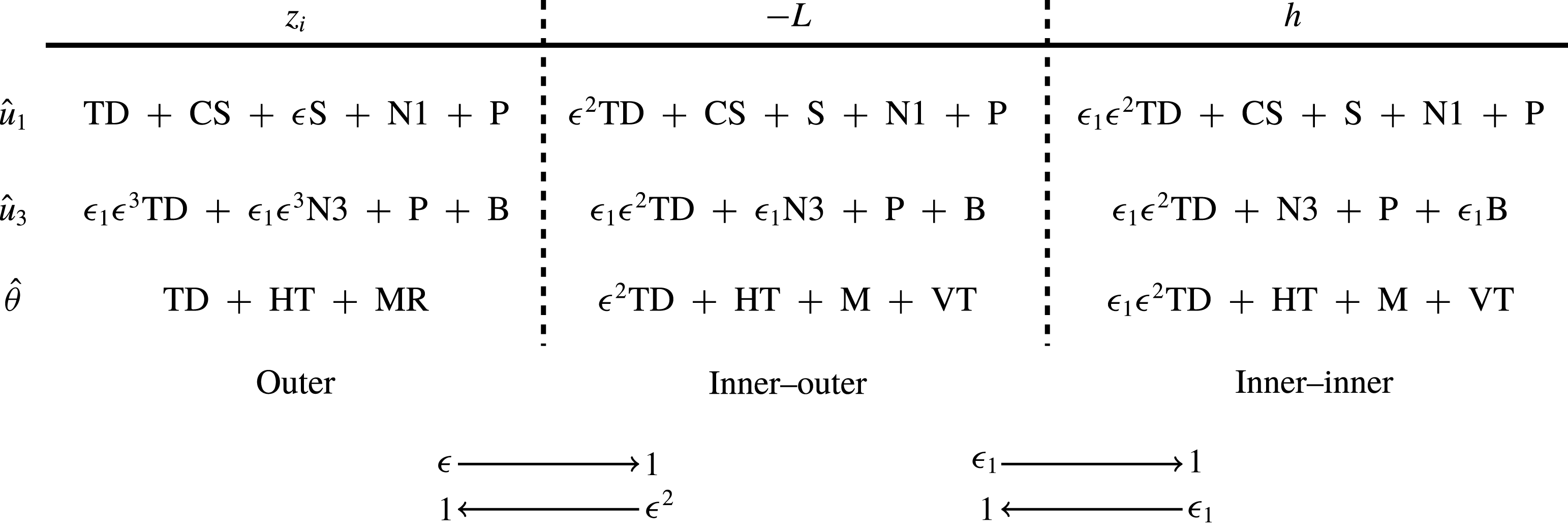
Diagram of the scaling regions, layers and ranges in the convective atmospheric surface layer.

For
 $z\gg -L$
and
 $k\lesssim 1/z$
(the convective layer in the Monin–Obukhov (M-O) region in figure 1), equations (2.3), (2.6) and (2.9) have the mixed-layer scaling and have leading-order solutions of the form
 $$\begin{eqnarray}\displaystyle \hat{u} _{1c}=\hat{u} _{1c}(k_{c},x_{3c}),\quad \hat{u} _{3c}=\hat{u} _{3c}(k_{c},x_{3c}),\quad \hat{\unicode[STIX]{x1D703}}_{c}=\hat{\unicode[STIX]{x1D703}}_{c}(k_{c},x_{3c}), & & \displaystyle\end{eqnarray}$$
since the mean-shear term in (2.3) and the terms on the LHS of (2.6) are small. The spectra in this layer have been predicted by Yaglom (Reference Yaglom1994). When
 $k_{c}$
increases in the convective layer (with
 $x_{3c}$
fixed), we enter the Kolmogorov region (this will be addressed in a separate study). In the present study we derive the MMO scaling in the convective–dynamic layer (
 $-z/L\ll 1$
). We note that when reducing the height from
 $z>-L$
to a height
 $z=h\ll -L$
, the term containing the small parameter in (2.3) becomes of order
 $u_{\ast }/w_{\ast }$
because
 $\unicode[STIX]{x2202}U/\unicode[STIX]{x2202}x_{3}\sim u_{\ast }/z$
(see (3.11) and the discussion there; it approaches
 $u_{\ast }/z(-z/L)^{-1/3}$
for
 $-z/L\gg 1$
(e.g. Wyngaard et al.
Reference Wyngaard, Coté and Izumi1971; Tong & Ding Reference Tong and Ding2018)), indicating that this (the mean-shear) term remains a higher-order term as
 $z$
becomes smaller than
 $-L$
(for the given
 $k_{c}<-1/L$
). The scaling of (2.3) also remains the same, indicating that the effects of the mean shear on the large scales remain small. Therefore the leading-order solution (2.10), which has the mixed-layer scaling, is still valid (i.e. uniformly valid, vertical arrows in figure 1) for
 $z\ll -L$
(the convective range). Thus the (higher-order) effects of the mean shear on the solutions
 $\hat{u} _{1c}$
,
 $\hat{u} _{3c}$
and
 $\hat{\unicode[STIX]{x1D703}}_{c}$
(for the given
 $k_{c}<-1/L$
) can be treated as a regular perturbation problem. Therefore, the starting point of (inputs into) our singular perturbation analysis is that in the convective–dynamic layer there exist the mixed-layer scaling with the velocity, temperature and length scales
 $w_{\ast }$
,
 $Q/w_{\ast }$
and
 $z_{i}$
, respectively, and the stress- and flux-carrying scaling with the friction velocity
 $u_{\ast }$
,
 $Q/w_{\ast }$
, and
 $z$
as the velocity, temperature and length scales, respectively. The two scales are effectively the outer scale and one of the inner scales of the problem.
In the convective–dynamic layer, when
 $k$
increases from the convective range (horizontal arrow in figure 1), at a fixed height, the mean-shear term in (1.2) increases with
 $k$
as
 $$\begin{eqnarray}\displaystyle \hat{u} _{3}\frac{\unicode[STIX]{x2202}U}{\unicode[STIX]{x2202}x_{3}}\sim u_{f}zk\frac{u_{\ast }}{z}=u_{f}u_{\ast }k\sim \left(\frac{g}{\unicode[STIX]{x1D6E9}}Q\right)^{1/3}u_{\ast }k^{2/3}, & & \displaystyle\end{eqnarray}$$
where
 $u_{f}x_{3}k$
is the magnitude of the vertical velocity fluctuations at scale
 $k$
, while the buoyancy term in (1.3) increases with
 $k$
as
 $$\begin{eqnarray}\displaystyle \frac{g}{\unicode[STIX]{x1D6E9}}\hat{\unicode[STIX]{x1D703}}\sim \frac{g}{\unicode[STIX]{x1D6E9}}\frac{Q}{u_{f}}\sim \left(\frac{g}{\unicode[STIX]{x1D6E9}}Q\right)^{2/3}k^{1/3}, & & \displaystyle\end{eqnarray}$$
indicating that the mean-shear term becomes increasingly important. It eventually becomes a leading-order term when equalling the buoyancy term:
 $$\begin{eqnarray}\displaystyle \left(\frac{g}{\unicode[STIX]{x1D6E9}}Q\right)^{1/3}u_{\ast }k^{2/3}\sim \left(\frac{g}{\unicode[STIX]{x1D6E9}}Q\right)^{2/3}k^{1/3},\quad \text{i.e. }k\sim \frac{g}{\unicode[STIX]{x1D6E9}}Qu_{\ast }^{-3}\sim -\frac{1}{L}. & & \displaystyle\end{eqnarray}$$
Since the mean-shear term has the (neutral) surface-layer scaling, the solution (2.10) is not valid when the mean-shear term is a leading-order term in (2.3), i.e. when the effect of the mean shear is important or dominant. This leads to a non-uniformly valid (outer) solution for
 $k_{c}>1$
, resulting in a singular perturbation problem. Therefore, the solution (2.10) is uniformly valid with respect to
 $x_{3c}$
(for
 $k_{c}<1$
), but not uniformly valid with respect to
 $k$
(e.g. as
 $k_{c}>1$
for
 $-z/L\ll 1$
). The non-uniformly valid solution indicates that there are two scaling ranges in which different physics dominates.
In the following we analyse the singular perturbation problem and
 $\hat{u} _{1}$
,
 $\hat{u} _{3}$
and
 $\hat{\unicode[STIX]{x1D703}}$
as functions of
 $k$
for a fixed
 $z=h\ll -L$
. (Therefore,
 $h$
is a parameter in the perturbation problem hereafter.) For convenience, we redefine the non-dimensional variables as outer variables as follows:
 $$\begin{eqnarray}\displaystyle \left.\begin{array}{@{}c@{}}\displaystyle \hat{u} _{1}=w_{\ast }\hat{u} _{1o},\quad \hat{u} _{3}=w_{\ast }\frac{h}{z_{i}}\hat{u} _{3o},\quad t=\frac{z_{i}}{w_{\ast }}\unicode[STIX]{x1D70F},\\ \displaystyle {\mathcal{L}}=z_{i}{\mathcal{L}}_{o},\quad \boldsymbol{k}=\frac{1}{z_{i}}\boldsymbol{k}_{o},\quad x_{3}=hx_{3o},\quad \hat{p}=w_{\ast }^{2}\hat{p}_{o},\\ \displaystyle \hat{\unicode[STIX]{x1D703}}=\frac{Q}{w_{\ast }}\hat{\unicode[STIX]{x1D703}}_{o},\quad \frac{\unicode[STIX]{x2202}\hat{p}}{\unicode[STIX]{x2202}x_{3}}=\left(\frac{\unicode[STIX]{x2202}\hat{p}}{\unicode[STIX]{x2202}x_{3}}\right)_{o}\frac{w_{\ast }^{2}}{h},\quad \frac{\unicode[STIX]{x2202}U}{\unicode[STIX]{x2202}x_{3}}=\frac{u^{\prime \prime }}{h}\left(\frac{\unicode[STIX]{x2202}U}{\unicode[STIX]{x2202}x_{3}}\right)_{o},\quad \frac{\unicode[STIX]{x2202}\unicode[STIX]{x1D6E9}}{\unicode[STIX]{x2202}x_{3}}=\frac{Q}{u_{\ast }h}\left(\frac{\unicode[STIX]{x2202}\unicode[STIX]{x1D6E9}}{\unicode[STIX]{x2202}x_{3}}\right)_{o}.\end{array}\right\} & & \displaystyle \nonumber\\ \displaystyle & & \displaystyle\end{eqnarray}$$
Here the non-dimensional forms of
 $\hat{u} _{3}$
and
 $x_{3}$
are of order one. Following equations (2.3), (2.6) and (2.9), we can write the outer equations as
 $$\begin{eqnarray}\displaystyle \left.\begin{array}{@{}c@{}}\displaystyle \frac{\bar{\text{D}}\hat{u} _{1o}}{\text{D}\unicode[STIX]{x1D70F}}+{\mathcal{L}}_{o}^{2}\int \hat{u} _{3o}\frac{\unicode[STIX]{x2202}\hat{u} _{1o}}{\unicode[STIX]{x2202}x_{3o}}\,\text{d}\boldsymbol{k}_{o}^{\prime }+\unicode[STIX]{x1D716}\hat{u} _{3o}\left(\frac{\unicode[STIX]{x2202}U}{\unicode[STIX]{x2202}x_{3}}\right)_{o}+{\mathcal{L}}_{o}^{2}\int \hat{u} _{1o}\text{i}k_{1o}^{\prime }\hat{u} _{1o}\,\text{d}\boldsymbol{k}_{o}^{\prime }=-\text{i}k_{1o}\hat{p_{o}},\\ \displaystyle \text{TD}\hspace{51.21504pt}\text{CS}\hspace{62.59596pt}\text{S}\hspace{85.35826pt}\text{N1}\hspace{62.59596pt}\text{P}\end{array}\right\} & & \displaystyle \nonumber\\ \displaystyle & & \displaystyle\end{eqnarray}$$
 $$\begin{eqnarray}\displaystyle \left.\begin{array}{@{}c@{}}\displaystyle \frac{h}{z_{i}}\frac{\bar{\text{D}}\hat{u} _{3o}}{\text{D}\unicode[STIX]{x1D70F}}+\frac{h}{z_{i}}\left({\mathcal{L}}_{o}^{2}\int \hat{u} _{3o}\frac{\unicode[STIX]{x2202}\hat{u} _{3o}}{\unicode[STIX]{x2202}x_{3o}}\,\text{d}\boldsymbol{k}_{o}^{\prime }+{\mathcal{L}}_{o}^{2}\int \hat{u} _{1o}\text{i}k_{1o}^{\prime }\hat{u} _{3o}\,\text{d}\boldsymbol{k}_{o}^{\prime }\right)=-\frac{z_{i}}{h}\left(\frac{\unicode[STIX]{x2202}\hat{p}}{\unicode[STIX]{x2202}x_{3}}\right)_{o}+\hat{\unicode[STIX]{x1D703}}_{o},\\ \displaystyle \text{TD}\hspace{122.34692pt}\text{N3}\hspace{125.19194pt}\text{P}\hspace{34.14322pt}\text{B}\end{array}\right\} & & \displaystyle \nonumber\\ \displaystyle & & \displaystyle\end{eqnarray}$$
 $$\begin{eqnarray}\displaystyle \left.\begin{array}{@{}l@{}}\displaystyle \frac{\bar{\text{D}}\hat{\unicode[STIX]{x1D703}}_{o}}{\text{D}\unicode[STIX]{x1D70F}}+{\mathcal{L}}_{o}^{2}\int \hat{u} _{1o}\text{i}k_{1o}^{\prime }\hat{\unicode[STIX]{x1D703}}_{o}\,\text{d}\boldsymbol{k}_{o}^{\prime }+\left(\frac{w_{\ast }}{u_{\ast }}\hat{u} _{3o}\left(\frac{\unicode[STIX]{x2202}\unicode[STIX]{x1D6E9}}{\unicode[STIX]{x2202}x_{3}}\right)_{o}+{\mathcal{L}}_{o}^{2}\int \hat{u} _{3o}\frac{\unicode[STIX]{x2202}\hat{\unicode[STIX]{x1D703}}_{o}}{\unicode[STIX]{x2202}x_{3o}}\,\text{d}\boldsymbol{k}_{o}^{\prime }\right)=0.\\ \displaystyle ~\text{TD}\hspace{54.06006pt}\text{HT}\hspace{113.81102pt}\text{MR}\end{array}\right\} & & \displaystyle \nonumber\\ \displaystyle & & \displaystyle\end{eqnarray}$$
Although there is a parameter
 $z_{i}/h$
in the pressure-gradient term in (2.16), this term is of order one. There is a small parameter in the time-derivative and nonlinear terms (N3) in the vertical velocity equation (2.16),
 $$\begin{eqnarray}\displaystyle \unicode[STIX]{x1D716}_{1}\unicode[STIX]{x1D716}^{3}=\frac{h}{z_{i}}=\frac{h}{L}\frac{L}{z_{i}}=-\frac{h}{L}\unicode[STIX]{x1D716}^{3}, & & \displaystyle\end{eqnarray}$$
where
 $\unicode[STIX]{x1D716}_{1}=-h/L$
, indicating that the LHS is of higher order. The small parameters
 $\unicode[STIX]{x1D716}$
and
 $\unicode[STIX]{x1D716}_{1}$
in (2.15) and (2.16) indicate that there are two inner ranges with different length scales (see (3.10)–(3.12)), resulting in a nested boundary layer problem in the spectral space. We call the ranges with the larger and smaller length scales the inner–outer range and the inner–inner range, respectively. We note that the terms containing the small parameter
 $\unicode[STIX]{x1D716}_{1}$
in (2.16) are not the source of non-uniformity of (2.10) since they remain higher-order terms as
 $k_{o}$
increases from
 $k_{o}<1$
to
 $k_{o}>1$
.
In the following analysis, we derive MMO for the horizontal Fourier transforms of the velocity and potential temperature, which are equivalent to the two-point velocity and temperature differences, without invoking the hypothesis in MMO.
Structure of the different scales in the surface layer including the dominant dynamic processes (terms). The arrows indicate the directions in which the terms containing the parameters change from small terms to order-one terms.

3 Matched asymptotic expansions
3.1 The outer expansions
The solution of equations (2.15), (2.16) and (2.17) can be written as series (outer) expansions in the powers of
 $\unicode[STIX]{x1D716}$
:
 $$\begin{eqnarray}\displaystyle \left.\begin{array}{@{}c@{}}\hat{u} _{1o}(\boldsymbol{k}_{o},x_{3o})=\hat{u} _{1o,1}+\unicode[STIX]{x1D716}\hat{u} _{1o,2}+O(\unicode[STIX]{x1D716}^{2}),\\ \hat{u} _{3o}(\boldsymbol{k}_{o},x_{3o})=\hat{u} _{3o,1}+\unicode[STIX]{x1D716}\hat{u} _{3o,2}+O(\unicode[STIX]{x1D716}^{2}),\\ \hat{\unicode[STIX]{x1D703}}_{o}(\boldsymbol{k}_{o},x_{3o})=\hat{\unicode[STIX]{x1D703}}_{o,1}+\unicode[STIX]{x1D716}\hat{\unicode[STIX]{x1D703}}_{o,2}+O(\unicode[STIX]{x1D716}^{2}).\end{array}\right\} & & \displaystyle\end{eqnarray}$$
As discussed above, the second-order terms are of order
 $\unicode[STIX]{x1D716}$
because they arise due to the mean-shear (production) term in (2.15). To illustrate more clearly the dynamic processes and the sources of non-uniformly valid solution, figure 2 provides a summary of the terms in (2.15), (2.16) and (2.17), and the terms containing small parameters. The arrows indicate the directions in which the terms containing the parameters change from small terms to order-one terms, i.e. the physics represented by the terms becomes dominant. The largest parameter
 $\unicode[STIX]{x1D716}$
rather than
 $\unicode[STIX]{x1D716}_{1}\unicode[STIX]{x1D716}$
is used in the second-order correction terms in the outer expansions (the latter corresponds to higher-order expansions).
3.2 The inner expansion
As discussed above, when the scale decreases (
 $k_{o}$
increases from
 $k_{o}\sim 1$
), the (small) mean-shear term in (2.15) will eventually become of order one, i.e. the shear production becomes important. Therefore, the outer expansions are no longer valid. New (inner) scales and non-dimensional (inner) variables are needed to obtain valid expansions. We define the non-dimensional inner variables as
 $$\begin{eqnarray}\displaystyle \left.\begin{array}{@{}c@{}}\displaystyle \hat{u} _{1}=u^{\prime }\hat{u} _{1in},\quad \hat{u} _{3}=u^{\prime }\frac{h}{\unicode[STIX]{x1D6FF}}\hat{u} _{3in},\quad {\mathcal{L}}=\unicode[STIX]{x1D6FF}{\mathcal{L}}_{in},\\ \displaystyle \boldsymbol{k}=\frac{1}{\unicode[STIX]{x1D6FF}}\boldsymbol{k}_{in},\quad x_{3}=hx_{3in}(x_{3in}=x_{3o}),\quad \hat{p}=u^{\prime 2}\hat{p}_{in},\\ \displaystyle \hat{\unicode[STIX]{x1D703}}=\frac{Q}{u^{\prime }}\hat{\unicode[STIX]{x1D703}}_{in},\quad \frac{\unicode[STIX]{x2202}\hat{p}}{\unicode[STIX]{x2202}x_{3}}=\frac{u^{\prime 2}}{h}\left(\frac{\unicode[STIX]{x2202}\hat{p}}{\unicode[STIX]{x2202}x_{3}}\right)_{in},\quad \frac{\unicode[STIX]{x2202}U}{\unicode[STIX]{x2202}x_{3}}=\frac{u^{\prime \prime }}{h}\left(\frac{\unicode[STIX]{x2202}U}{\unicode[STIX]{x2202}x_{3}}\right)_{in},\quad \frac{\unicode[STIX]{x2202}\unicode[STIX]{x1D6E9}}{\unicode[STIX]{x2202}x_{3}}=\frac{Q}{u_{\ast }h}\left(\frac{\unicode[STIX]{x2202}\unicode[STIX]{x1D6E9}}{\unicode[STIX]{x2202}x_{3}}\right)_{in},\end{array}\right\} & & \displaystyle \nonumber\\ \displaystyle & & \displaystyle\end{eqnarray}$$
where
 $u^{\prime }$
and
 $\unicode[STIX]{x1D6FF}$
are the inner velocity and length scales, respectively, all yet to be determined. Substituting these variables into the horizontal velocity equation results in
 $$\begin{eqnarray}\displaystyle & & \displaystyle \frac{\bar{\text{D}}\hat{u} _{1in}}{\text{D}\unicode[STIX]{x1D70F}}u^{\prime }\frac{w_{\ast }}{z_{i}}+\unicode[STIX]{x1D6FF}^{2}{\mathcal{L}}_{in}^{2}\int \hat{u} _{3in}\frac{\unicode[STIX]{x2202}\hat{u} _{1in}}{\unicode[STIX]{x2202}x_{3in}}\,\text{d}\boldsymbol{k}_{in}^{\prime }\,u^{\prime }\frac{h}{\unicode[STIX]{x1D6FF}}\frac{u^{\prime }}{h}\frac{1}{\unicode[STIX]{x1D6FF}^{2}}+\hat{u} _{3in}\left(\frac{\unicode[STIX]{x2202}U}{\unicode[STIX]{x2202}x_{3}}\right)_{in}u^{\prime }\frac{h}{\unicode[STIX]{x1D6FF}}\frac{u^{\prime \prime }}{h}\nonumber\\ \displaystyle & & \displaystyle \quad +\,\unicode[STIX]{x1D6FF}^{2}{\mathcal{L}}_{in}^{2}\int \hat{u} _{1in}\text{i}k_{1in}^{\prime }\hat{u} _{1in}\,\text{d}\boldsymbol{k}_{in}^{\prime }\,u^{\prime 2}\frac{1}{\unicode[STIX]{x1D6FF}^{3}}=-\text{i}k_{1in}\hat{p}_{in}\frac{u^{\prime 2}}{\unicode[STIX]{x1D6FF}}.\end{eqnarray}$$
Dividing this equation by
 $u^{\prime 2}/\unicode[STIX]{x1D6FF}$
gives
 $$\begin{eqnarray}\displaystyle & & \displaystyle \frac{w_{\ast }}{u^{\prime }}\frac{\unicode[STIX]{x1D6FF}}{z_{i}}\frac{\bar{\text{D}}\hat{u} _{1in}}{\text{D}\unicode[STIX]{x1D70F}}+{\mathcal{L}}_{in}^{2}\int \hat{u} _{3in}\frac{\unicode[STIX]{x2202}\hat{u} _{1in}}{\unicode[STIX]{x2202}x_{3in}}\,\text{d}\boldsymbol{k}_{in}^{\prime }+\frac{u^{\prime \prime }}{u^{\prime }}\hat{u} _{3in}\left(\frac{\unicode[STIX]{x2202}U}{\unicode[STIX]{x2202}x_{3}}\right)_{in}\nonumber\\ \displaystyle & & \displaystyle \quad +\,{\mathcal{L}}_{in}^{2}\int \hat{u} _{1in}\text{i}k_{1in}^{\prime }\hat{u} _{1in}\,\text{d}\boldsymbol{k}_{in}^{\prime }=-\text{i}k_{1in}\hat{p}_{in}.\end{eqnarray}$$
At the inner scale
 $k\sim 1/\unicode[STIX]{x1D6FF}$
(
 $k_{in}\sim 1$
), the mean shear must be a leading-order term, along with the pressure-gradient terms in (3.4),
 $$\begin{eqnarray}\displaystyle \hat{u} _{3}\frac{\unicode[STIX]{x2202}U}{\unicode[STIX]{x2202}x_{3}}\sim -\text{i}k_{1}\hat{p}, & & \displaystyle\end{eqnarray}$$
resulting in
 $u^{\prime \prime }=u^{\prime }$
. Thus the mean-shear term has the same velocity scale as the fluctuating velocity.
The inner vertical velocity equation becomes
 $$\begin{eqnarray}\displaystyle & & \displaystyle \frac{\bar{\text{D}}\hat{u} _{3in}}{\text{D}\unicode[STIX]{x1D70F}}u^{\prime }\frac{h}{\unicode[STIX]{x1D6FF}}\frac{w_{\ast }}{z_{i}}+\unicode[STIX]{x1D6FF}^{2}{\mathcal{L}}_{in}^{2}\int \hat{u} _{3in}\frac{\unicode[STIX]{x2202}\hat{u} _{3in}}{\unicode[STIX]{x2202}x_{3in}}\,\text{d}\boldsymbol{k}_{in}^{\prime }\,u^{\prime 2}\frac{h^{2}}{\unicode[STIX]{x1D6FF}^{2}}\frac{1}{h}\frac{1}{\unicode[STIX]{x1D6FF}^{2}}+\unicode[STIX]{x1D6FF}^{2}{\mathcal{L}}_{in}^{2}\int \hat{u} _{1in}\text{i}k_{1in}^{\prime }\hat{u} _{3in}\,\text{d}\boldsymbol{k}_{in}^{\prime }\,u^{\prime 2}\frac{h}{\unicode[STIX]{x1D6FF}}\frac{1}{\unicode[STIX]{x1D6FF}^{3}}\nonumber\\ \displaystyle & & \displaystyle \quad =-\left(\frac{\unicode[STIX]{x2202}\hat{p}}{\unicode[STIX]{x2202}x_{3}}\right)_{in}\frac{u^{\prime 2}}{h}+\frac{g}{\unicode[STIX]{x1D6E9}}\frac{Q}{u^{\prime }}\hat{\unicode[STIX]{x1D703}}_{in}.\end{eqnarray}$$
Again dividing by
 $u^{\prime 2}/\unicode[STIX]{x1D6FF}$
results in
 $$\begin{eqnarray}\displaystyle & & \displaystyle \frac{w_{\ast }}{u^{\prime }}\frac{h}{z_{i}}\frac{\bar{\text{D}}\hat{u} _{3in}}{\text{D}\unicode[STIX]{x1D70F}}+\frac{h}{\unicode[STIX]{x1D6FF}}\left({\mathcal{L}}_{in}^{2}\int \hat{u} _{3in}\frac{\unicode[STIX]{x2202}\hat{u} _{3in}}{\unicode[STIX]{x2202}x_{3in}}\,\text{d}\boldsymbol{k}_{in}^{\prime }+{\mathcal{L}}_{in}^{2}\int \hat{u} _{1in}\text{i}k_{1in}^{\prime }\hat{u} _{3in}\,\text{d}\boldsymbol{k}_{in}^{\prime }\right)\nonumber\\ \displaystyle & & \displaystyle \quad =-\frac{\unicode[STIX]{x1D6FF}}{h}\left(\frac{\unicode[STIX]{x2202}\hat{p}}{\unicode[STIX]{x2202}x_{3}}\right)_{in}+\frac{g}{\unicode[STIX]{x1D6E9}}\frac{Q}{u^{\prime 3}}\unicode[STIX]{x1D6FF}\hat{\unicode[STIX]{x1D703}}_{in}.\end{eqnarray}$$
Again, the pressure-gradient term in (3.7) is of order one. The inner temperature equation becomes
 $$\begin{eqnarray}\displaystyle & & \displaystyle \frac{\bar{\text{D}}\hat{\unicode[STIX]{x1D703}}_{in}}{\text{D}\unicode[STIX]{x1D70F}}\frac{Q}{u_{\ast }}\frac{w_{\ast }}{z_{i}}+\unicode[STIX]{x1D6FF}^{2}{\mathcal{L}}_{in}^{2}\int \hat{u} _{1in}\text{i}k_{1in}^{\prime }\hat{\unicode[STIX]{x1D703}}_{in}\,\text{d}\boldsymbol{k}_{in}^{\prime }\,u_{\ast }\frac{1}{\unicode[STIX]{x1D6FF}}\frac{Q}{u_{\ast }}\frac{1}{\unicode[STIX]{x1D6FF}^{2}}+\hat{u} _{3in}\left(\frac{\unicode[STIX]{x2202}\unicode[STIX]{x1D6E9}}{\unicode[STIX]{x2202}x_{3}}\right)_{in}u_{\ast }\frac{h}{\unicode[STIX]{x1D6FF}}\frac{Q}{u_{\ast }h}\nonumber\\ \displaystyle & & \displaystyle \quad +\,\unicode[STIX]{x1D6FF}^{2}{\mathcal{L}}_{in}^{2}\int \hat{u} _{3in}\frac{\unicode[STIX]{x2202}\hat{\unicode[STIX]{x1D703}}_{in}}{\unicode[STIX]{x2202}x_{3in}}\,\text{d}\boldsymbol{k}_{in}^{\prime }\,u_{\ast }\frac{h}{\unicode[STIX]{x1D6FF}}\frac{Q}{u_{\ast }h}\frac{1}{\unicode[STIX]{x1D6FF}^{2}}=0.\end{eqnarray}$$
Similarly dividing by
 $Q/\unicode[STIX]{x1D6FF}$
results in
 $$\begin{eqnarray}\displaystyle \frac{w_{\ast }}{u_{\ast }}\frac{\unicode[STIX]{x1D6FF}}{z_{i}}\frac{\bar{\text{D}}\hat{\unicode[STIX]{x1D703}}_{in}}{\text{D}\unicode[STIX]{x1D70F}}+{\mathcal{L}}_{in}^{2}\int \hat{u} _{1in}\text{i}k_{1in}^{\prime }\hat{\unicode[STIX]{x1D703}}_{in}\,\text{d}\boldsymbol{k}_{in}^{\prime }+\hat{u} _{3in}\left(\frac{\unicode[STIX]{x2202}\unicode[STIX]{x1D6E9}}{\unicode[STIX]{x2202}x_{3}}\right)_{in}+{\mathcal{L}}_{in}^{2}\int \hat{u} _{3in}\frac{\unicode[STIX]{x2202}\hat{\unicode[STIX]{x1D703}}_{in}}{\unicode[STIX]{x2202}x_{3in}}\,\text{d}\boldsymbol{k}_{in}^{\prime }=0. & & \displaystyle\end{eqnarray}$$
Determination of
 $\unicode[STIX]{x1D6FF}$
from (3.7) requires the notion of distinguished limit, which involves a dominant-balance argument. There are two possibilities to consider:
 $$\begin{eqnarray}\displaystyle \left.\begin{array}{@{}l@{}}\displaystyle (1)\quad \frac{h}{\unicode[STIX]{x1D6FF}}\sim 1,\\ \displaystyle (2)\quad \frac{g}{\unicode[STIX]{x1D6E9}}\frac{Q}{u^{\prime 3}}\unicode[STIX]{x1D6FF}\sim 1.\end{array}\right\} & & \displaystyle\end{eqnarray}$$
In the first case (
 $\unicode[STIX]{x1D6FF}=h$
), the nonlinear terms on the LHS of (3.7) are of order one, balancing the pressure gradient
 $\unicode[STIX]{x2202}\hat{p}/\unicode[STIX]{x2202}x_{3}$
. Since the shear-stress-carrying eddies have length and velocity scales of
 $h$
and
 $u_{\ast }$
, respectively, from (3.2) we have
 $$\begin{eqnarray}\displaystyle u^{\prime }(=u^{\prime \prime })=u_{\ast }, & & \displaystyle\end{eqnarray}$$
and thus the mean velocity gradient
 $\unicode[STIX]{x2202}U/\unicode[STIX]{x2202}x_{3}$
scales as
 $u_{\ast }/h$
. The buoyancy term
 $\hat{\unicode[STIX]{x1D703}}$
is a second-order term in this case, i.e. the buoyancy effects are small. We define this scale as the inner–inner scale.
In the second case (
 $\unicode[STIX]{x1D6FF}=u^{\prime 3}/(gQ/\unicode[STIX]{x1D6E9})$
), to the leading order,
 $\unicode[STIX]{x2202}\hat{p}/\unicode[STIX]{x2202}x_{3}$
and
 $\hat{\unicode[STIX]{x1D703}}$
balance each other; therefore the LHS of (3.7) is of second order. Since
 $\unicode[STIX]{x2202}U/\unicode[STIX]{x2202}x_{3}$
scales as
 $u_{\ast }/h$
, the velocity scale
 $u^{\prime \prime }(=u^{\prime })=u_{\ast }$
, the same as in the first case, which leads to
 $$\begin{eqnarray}\displaystyle \unicode[STIX]{x1D6FF}=u_{\ast }^{3}/(gQ/\unicode[STIX]{x1D6E9})\sim -L, & & \displaystyle\end{eqnarray}$$
i.e. the inner length scale is the Obukhov length, which is a result of the buoyancy force balancing the pressure force. This result is of key importance and provides an analytical proof that
 $L$
is not only a vertical length scale, as in the MOST (Obukhov Reference Obukhov1946; Monin & Obukhov Reference Monin and Obukhov1954; Tong & Ding Reference Tong and Ding2018), but also a horizontal length scale, as hypothesized in MMO (Tong & Nguyen Reference Tong and Nguyen2015). We define this scale as the inner–outer scale. For scales with
 $k<-1/L$
, buoyancy and pressure gradient dominate, whereas for
 $k>-1/L$
, shear and pressure gradient dominate.
3.3 The inner–outer expansion
With
 $u_{\ast }$
and
 $L$
being the velocity and length scales for the inner–outer range, we write the non-dimensional velocity and temperature equations as
 $$\begin{eqnarray}\displaystyle \left.\begin{array}{@{}c@{}}\displaystyle \unicode[STIX]{x1D716}^{2}\frac{\bar{\text{D}}\hat{u} _{1io}}{\text{D}\unicode[STIX]{x1D70F}}+{\mathcal{L}}_{io}^{2}\int \hat{u} _{3io}\frac{\unicode[STIX]{x2202}\hat{u} _{1io}}{\unicode[STIX]{x2202}x_{3io}}\,\text{d}\boldsymbol{k}_{io}^{\prime }+\hat{u} _{3io}\left(\frac{\unicode[STIX]{x2202}U}{\unicode[STIX]{x2202}x_{3}}\right)_{io}+{\mathcal{L}}_{io}^{2}\int \hat{u} _{1io}\text{i}k_{1io}^{\prime }\hat{u} _{1io}\,\text{d}\boldsymbol{k}_{io}^{\prime }=-\text{i}k_{1io}\hat{p}_{io},\\ \displaystyle \hspace{11.38092pt}\text{TD}\hspace{62.59596pt}\text{CS}\hspace{65.44142pt}\text{S}\hspace{93.89418pt}\text{N1}\hspace{62.59596pt}\text{P}\end{array}\right\} & & \displaystyle \nonumber\\ \displaystyle & & \displaystyle\end{eqnarray}$$
 $$\begin{eqnarray}\displaystyle \left.\begin{array}{@{}c@{}}\displaystyle \!\!\unicode[STIX]{x1D716}_{1}\unicode[STIX]{x1D716}^{2}\frac{\bar{\text{D}}\hat{u} _{3io}}{\text{D}\unicode[STIX]{x1D70F}}+\unicode[STIX]{x1D716}_{1}\left(\!{\mathcal{L}}_{io}^{2}\int \hat{u} _{3io}\frac{\unicode[STIX]{x2202}\hat{u} _{3io}}{\unicode[STIX]{x2202}x_{3io}}\,\text{d}\boldsymbol{k}_{io}^{\prime }+{\mathcal{L}}_{io}^{2}\int \hat{u} _{1io}\text{i}k_{1io}^{\prime }\hat{u} _{3io}\,\text{d}\boldsymbol{k}_{io}^{\prime }\right)=-\frac{1}{\unicode[STIX]{x1D716}_{1}}\left(\frac{\unicode[STIX]{x2202}\hat{p}}{\unicode[STIX]{x2202}x_{3}}\right)_{io}\!+\hat{\unicode[STIX]{x1D703}}_{io},\\ \displaystyle \hspace{11.38092pt}\text{TD}\hspace{136.5733pt}\text{N3}\hspace{139.41832pt}\text{P}\hspace{31.2982pt}\text{B}\end{array}\right\} & & \displaystyle \nonumber\\ \displaystyle & & \displaystyle\end{eqnarray}$$
 $$\begin{eqnarray}\displaystyle \left.\begin{array}{@{}l@{}}\displaystyle \unicode[STIX]{x1D716}^{2}\frac{\bar{\text{D}}\hat{\unicode[STIX]{x1D703}}_{io}}{\text{D}\unicode[STIX]{x1D70F}}+{\mathcal{L}}_{io}^{2}\int \hat{u} _{1io}\text{i}k_{1io}^{\prime }\hat{\unicode[STIX]{x1D703}}_{io}\,\text{d}\boldsymbol{k}_{io}^{\prime }+\hat{u} _{3io}\left(\frac{\unicode[STIX]{x2202}\unicode[STIX]{x1D6E9}}{\unicode[STIX]{x2202}x_{3}}\right)_{io}+{\mathcal{L}}_{io}^{2}\int \hat{u} _{3io}\frac{\unicode[STIX]{x2202}\hat{\unicode[STIX]{x1D703}}_{io}}{\unicode[STIX]{x2202}x_{3io}}\,\text{d}\boldsymbol{k}_{io}^{\prime }=0,\\ \displaystyle ~~~\text{TD}\hspace{56.9055pt}\text{HT}\hspace{73.97733pt}\text{M}\hspace{79.6678pt}\text{VT}\end{array}\right\}\qquad & & \displaystyle \nonumber\\ \displaystyle & & \displaystyle\end{eqnarray}$$
where the terms denoted as M and VT are the mean gradient production and the vertical transport, respectively. Note that at a height
 $h\ll 1/k$
, although the buoyancy force is of the same order of magnitude as the pressure gradient (
 $(g/\unicode[STIX]{x1D6E9})(Q/u_{f})\sim u_{f}^{2}k$
), the buoyancy production is smaller than the pressure–strain rate correlation (
 $(g/\unicode[STIX]{x1D6E9})(Q/u_{f})u_{f}hk\ll u_{f}^{3}k$
).
There are two sets of inner–outer expansions, with the same first-order terms. One is the ‘inner’ expansions to be matched with the outer expansions:
 $$\begin{eqnarray}\displaystyle \left.\begin{array}{@{}c@{}}\hat{u} _{1io}(\boldsymbol{k}_{io},x_{3io})=\hat{u} _{1io,1}+\unicode[STIX]{x1D716}^{2}\hat{u} _{1io,2}+O(\unicode[STIX]{x1D716}^{4}),\\ \hat{u} _{3io}(\boldsymbol{k}_{io},x_{3io})=\hat{u} _{3io,1}+\unicode[STIX]{x1D716}^{2}\hat{u} _{3io,2}+O(\unicode[STIX]{x1D716}^{4}),\\ \hat{\unicode[STIX]{x1D703}}_{io}(\boldsymbol{k}_{io},x_{3io})=\hat{\unicode[STIX]{x1D703}}_{io,1}+\unicode[STIX]{x1D716}^{2}\hat{\unicode[STIX]{x1D703}}_{io,2}+O(\unicode[STIX]{x1D716}^{4}).\end{array}\right\} & & \displaystyle\end{eqnarray}$$
The second-order terms are due to the time-derivative terms (order
 $\unicode[STIX]{x1D716}^{2}$
),
 $\bar{\text{D}}\hat{u} _{1io}/\text{D}\unicode[STIX]{x1D70F}$
and
 $\bar{\text{D}}\hat{\unicode[STIX]{x1D703}}_{io}/\text{D}\unicode[STIX]{x1D70F}$
, which become order-one terms as
 $k\rightarrow 1/z_{i}$
, i.e. the external influences (e.g. unsteadiness) become important. The other set of inner–outer expansions is the ‘outer’ expansions to be matched with the inner–inner expansions (discussed in the following):
 $$\begin{eqnarray}\displaystyle \left.\begin{array}{@{}c@{}}\hat{u} _{1io}(\boldsymbol{k}_{io},x_{3io})=\hat{u} _{1io,1}+\unicode[STIX]{x1D716}_{1}\hat{u} _{1io,2}^{\prime }+O(\unicode[STIX]{x1D716}_{1}^{2}),\\ \hat{u} _{3io}(\boldsymbol{k}_{io},x_{3io})=\hat{u} _{3io,1}+\unicode[STIX]{x1D716}_{1}\hat{u} _{3io,2}^{\prime }+O(\unicode[STIX]{x1D716}_{1}^{2}),\\ \hat{\unicode[STIX]{x1D703}}_{io}(\boldsymbol{k}_{io},x_{3io})=\hat{\unicode[STIX]{x1D703}}_{io,1}+\unicode[STIX]{x1D716}_{1}\hat{\unicode[STIX]{x1D703}}_{io,2}^{\prime }+O(\unicode[STIX]{x1D716}_{1}^{2}).\end{array}\right\} & & \displaystyle\end{eqnarray}$$
Here the second-order terms arise due to the nonlinear terms (order
 $\unicode[STIX]{x1D716}_{1}$
) in the
 $\hat{u} _{3io}$
equation (3.14), and represent spectral transfer of the
 $\hat{u} _{3}$
fluctuations from scales
 $h$
to smaller scales, and become of order one as
 $k\rightarrow 1/h$
. The leading-order terms in the expansions in (3.16) and (3.17) are only functions of the inner–outer wavenumber
 $k_{io}=-kL$
. This is a key result, proving the main hypothesis of MMO for two-point horizontal separations.
3.4 The inner–inner expansion
With
 $u_{\ast }$
and
 $h$
being the velocity and length scales for the inner–inner range, we write the non-dimensional velocity and temperature equations as
 $$\begin{eqnarray}\displaystyle \left.\begin{array}{@{}c@{}}\displaystyle \unicode[STIX]{x1D716}_{1}\unicode[STIX]{x1D716}^{2}\frac{\bar{\text{D}}\hat{u} _{1ii}}{\text{D}\unicode[STIX]{x1D70F}}+{\mathcal{L}}_{ii}^{2}\int \hat{u} _{3ii}\frac{\unicode[STIX]{x2202}\hat{u} _{1ii}}{\unicode[STIX]{x2202}x_{3ii}}\,\text{d}\boldsymbol{k}_{ii}^{\prime }+\hat{u} _{3ii}\left(\frac{\unicode[STIX]{x2202}U}{\unicode[STIX]{x2202}x_{3}}\right)_{ii}+{\mathcal{L}}_{ii}^{2}\int \hat{u} _{1ii}\text{i}k_{1ii}^{\prime }\hat{u} _{1ii}\,\text{d}\boldsymbol{k}_{ii}^{\prime }=-\text{i}k_{1ii}\hat{p}_{ii},\\ \displaystyle \hspace{11.38092pt}\text{TD}\hspace{62.59596pt}\text{CS}\hspace{65.44142pt}\text{S}\hspace{85.35826pt}\text{N1}\hspace{62.59596pt}\text{P}\end{array}\right\}\quad & & \displaystyle \nonumber\\ \displaystyle & & \displaystyle\end{eqnarray}$$
 $$\begin{eqnarray}\displaystyle \left.\begin{array}{@{}c@{}}\displaystyle \unicode[STIX]{x1D716}_{1}\unicode[STIX]{x1D716}^{2}\frac{\bar{\text{D}}\hat{u} _{3ii}}{\text{D}\unicode[STIX]{x1D70F}}+\left({\mathcal{L}}_{ii}^{2}\int \hat{u} _{3ii}\frac{\unicode[STIX]{x2202}\hat{u} _{3ii}}{\unicode[STIX]{x2202}x_{3ii}}\,\text{d}\boldsymbol{k}_{ii}^{\prime }+{\mathcal{L}}_{ii}^{2}\int \hat{u} _{1ii}\text{i}k_{1ii}^{\prime }\hat{u} _{3ii}\,\text{d}\boldsymbol{k}_{ii}^{\prime }\right)=-\left(\frac{\unicode[STIX]{x2202}\hat{p}}{\unicode[STIX]{x2202}x_{3}}\right)_{ii}+\unicode[STIX]{x1D716}_{1}\hat{\unicode[STIX]{x1D703}}_{ii},\\ \displaystyle \hspace{11.38092pt}\text{TD}\hspace{119.50148pt}\text{N3}\hspace{133.72786pt}\text{P}\hspace{28.45274pt}\text{B}\end{array}\right\}\quad & & \displaystyle \nonumber\\ \displaystyle & & \displaystyle\end{eqnarray}$$
 $$\begin{eqnarray}\displaystyle \left.\begin{array}{@{}l@{}}\displaystyle \unicode[STIX]{x1D716}_{1}\unicode[STIX]{x1D716}^{2}\frac{\bar{\text{D}}\hat{\unicode[STIX]{x1D703}}_{ii}}{\text{D}\unicode[STIX]{x1D70F}}+{\mathcal{L}}_{ii}^{2}\int \hat{u} _{1ii}\text{i}k_{1ii}^{\prime }\hat{\unicode[STIX]{x1D703}}_{ii}\,\text{d}\boldsymbol{k}_{ii}^{\prime }+\hat{u} _{3ii}\left(\frac{\unicode[STIX]{x2202}\unicode[STIX]{x1D6E9}}{\unicode[STIX]{x2202}x_{3}}\right)_{ii}+{\mathcal{L}}_{ii}^{2}\int \hat{u} _{3ii}\frac{\unicode[STIX]{x2202}\hat{\unicode[STIX]{x1D703}}_{ii}}{\unicode[STIX]{x2202}x_{3ii}}\,\text{d}\boldsymbol{k}_{ii}^{\prime }=0.\\ \displaystyle ~~~\text{TD}\hspace{65.44142pt}\text{HT}\hspace{56.9055pt}\text{M}\hspace{68.28644pt}\text{VT}\end{array}\right\}\qquad & & \displaystyle\end{eqnarray}$$
The inner–inner expansions therefore are
 $$\begin{eqnarray}\displaystyle \left.\begin{array}{@{}c@{}}\hat{u} _{1ii}(\boldsymbol{k}_{ii},x_{3ii})=\hat{u} _{1ii,1}+\unicode[STIX]{x1D716}_{1}\hat{u} _{1ii,2}+O(\unicode[STIX]{x1D716}_{1}^{2}),\\ \hat{u} _{3ii}(\boldsymbol{k}_{ii},x_{3ii})=\hat{u} _{3ii,1}+\unicode[STIX]{x1D716}_{1}\hat{u} _{3ii,2}+O(\unicode[STIX]{x1D716}_{1}^{2}),\\ \hat{\unicode[STIX]{x1D703}}_{ii}(\boldsymbol{k}_{ii},x_{3ii})=\hat{\unicode[STIX]{x1D703}}_{ii,1}+\unicode[STIX]{x1D716}_{1}\hat{\unicode[STIX]{x1D703}}_{ii,2}+O(\unicode[STIX]{x1D716}_{1}^{2}).\end{array}\right\} & & \displaystyle\end{eqnarray}$$
The second-order terms arise due to the buoyancy terms (order
 $\unicode[STIX]{x1D716}_{1}$
) in (3.19), which become of order one as
 $k\rightarrow -1/L$
, representing the deviation to the scaling in the dynamic range due to buoyancy.
3.5 Matching between the outer and inner–outer expansions
We now perform asymptotic matching between the outer and inner–outer ranges to obtain the leading-order terms in the overlapping region of the two ranges. The inner–outer expansion of the outer expansion of
 $\hat{u} _{1}$
is
 $$\begin{eqnarray}\displaystyle \hat{u} _{1} & = & \displaystyle w_{\ast }\left(\hat{u} _{1o,1}\left(-\frac{z_{i}}{L}\boldsymbol{k}_{io}\right)+\unicode[STIX]{x1D716}\hat{u} _{1o,2}\left(-\frac{z_{i}}{L}\boldsymbol{k}_{io}\right)+O(\unicode[STIX]{x1D716}^{2})\right)\nonumber\\ \displaystyle & {\sim} & \displaystyle u_{\ast }\left(-\frac{z_{i}}{L}\right)^{1/3}\hat{u} _{1o,1}\left(-\frac{z_{i}}{L}\boldsymbol{k}_{io}\right),\quad \text{as }\unicode[STIX]{x1D716}\rightarrow 0,\text{with }\boldsymbol{k}_{io}\text{ fixed},\nonumber\\ \displaystyle & {\sim} & \displaystyle u_{\ast }\left(-\frac{z_{i}}{L}\right)^{1/3}\left(-\frac{z_{i}}{L}k_{io}\right)^{\unicode[STIX]{x1D6FC}}\frac{1}{(L{\mathcal{L}}_{io})/z_{i}},\quad \text{as }\boldsymbol{k}_{io}\rightarrow \infty ,\end{eqnarray}$$
keeping only one term. Note that in the last step
 $1/{\mathcal{L}}_{o}=1/(L{\mathcal{L}}_{io}/z_{i})$
is included in the power-law dependence because a two-dimensional Fourier transform is proportional to
 $(\unicode[STIX]{x0394}k_{1}\unicode[STIX]{x0394}k_{2})^{1/2}\sim 1/{\mathcal{L}}$
(Monin & Yaglom Reference Monin and Yaglom1975).
The outer expansion of the inner–outer expansion of
 $\hat{u} _{1}$
is
 $$\begin{eqnarray}\displaystyle \hat{u} _{1} & = & \displaystyle u_{\ast }\left(\hat{u} _{1io,1}\left(-\frac{L}{z_{i}}\boldsymbol{k}_{o}\right)+\unicode[STIX]{x1D716}^{2}\hat{u} _{1io,2}\left(-\frac{L}{z_{i}}\boldsymbol{k}_{o}\right)+O(\unicode[STIX]{x1D716}^{4})\right)\nonumber\\ \displaystyle & {\sim} & \displaystyle w_{\ast }\left(-\frac{L}{z_{i}}\right)^{1/3}\hat{u} _{1io,1}\left(-\frac{L}{z_{i}}\boldsymbol{k}_{o}\right),\quad \text{as }\unicode[STIX]{x1D716}^{2}\rightarrow 0,\text{with }\boldsymbol{k}_{o}\text{ fixed},\nonumber\\ \displaystyle & {\sim} & \displaystyle u_{\ast }(k_{io})^{\unicode[STIX]{x1D6FC}}\frac{1}{{\mathcal{L}}_{io}},\quad \text{as }\boldsymbol{k}_{o}\rightarrow 0,\end{eqnarray}$$
also keeping only one term.
Matching (3.22) and (3.23) results in
 $\unicode[STIX]{x1D6FC}=-4/3$
. Thus,
 $$\begin{eqnarray}\displaystyle \hat{u} _{1o,1}\sim k_{o}^{-4/3}\frac{1}{{\mathcal{L}}_{o}}, & & \displaystyle\end{eqnarray}$$
and therefore the two-dimensional spectrum is
 $$\begin{eqnarray}\displaystyle \unicode[STIX]{x1D719}_{1o,1}={\mathcal{L}}_{o}^{2}\langle \hat{u} _{1o,1}\hat{u} _{1o,1}^{\ast }\rangle \sim k_{o}^{-8/3}. & & \displaystyle\end{eqnarray}$$
The spectrum integrated over a ring
 $|\boldsymbol{k}_{o}|=k_{o}$
has a
 $k_{o}^{-5/3}$
dependence, the same as the MMO prediction (Tong & Nguyen Reference Tong and Nguyen2015).
The inner–outer expansion of the outer expansion of
 $\hat{u} _{3}$
is
 $$\begin{eqnarray}\displaystyle \hat{u} _{3} & = & \displaystyle w_{\ast }\frac{h}{z_{i}}\left(\hat{u} _{3o,1}\left(-\frac{z_{i}}{L}\boldsymbol{k}_{io}\right)+\unicode[STIX]{x1D716}\hat{u} _{3o,2}\left(-\frac{z_{i}}{L}\boldsymbol{k}_{io}\right)+O(\unicode[STIX]{x1D716}^{2})\right)\nonumber\\ \displaystyle & {\sim} & \displaystyle u_{\ast }\left(-\frac{z_{i}}{L}\right)^{1/3}\frac{h}{z_{i}}\hat{u} _{3o,1}\left(-\frac{z_{i}}{L}\boldsymbol{k}_{io}\right),\quad \text{as }\unicode[STIX]{x1D716}\rightarrow 0,\text{with }\boldsymbol{k}_{io}\text{ fixed},\nonumber\\ \displaystyle & {\sim} & \displaystyle u_{\ast }\left(-\frac{z_{i}}{L}\right)^{1/3}\frac{h}{z_{i}}\left(-\frac{z_{i}}{L}k_{io}\right)^{\unicode[STIX]{x1D6FD}}\frac{1}{(L{\mathcal{L}}_{io})/z_{i}},\quad \text{as }\boldsymbol{k}_{io}\rightarrow \infty ,\end{eqnarray}$$
keeping only one term.
The outer expansion of the inner–outer expansion of
 $\hat{u} _{3}$
is
 $$\begin{eqnarray}\displaystyle \hat{u} _{3} & = & \displaystyle u_{\ast }\frac{h}{L}\left(\hat{u} _{3io,1}\left(-\frac{L}{z_{i}}\boldsymbol{k}_{o}\right)+\unicode[STIX]{x1D716}^{2}\hat{u} _{3io,2}\left(-\frac{L}{z_{i}}\boldsymbol{k}_{o}\right)+O(\unicode[STIX]{x1D716}^{4})\right)\nonumber\\ \displaystyle & {\sim} & \displaystyle w_{\ast }\left(-\frac{L}{z_{i}}\right)^{1/3}\frac{h}{L}\hat{u} _{3io,1}\left(-\frac{L}{z_{i}}\boldsymbol{k}_{o}\right),\quad \text{as }\unicode[STIX]{x1D716}^{2}\rightarrow 0,\text{with }\boldsymbol{k}_{o}\text{ fixed},\nonumber\\ \displaystyle & {\sim} & \displaystyle u_{\ast }\frac{h}{L}k_{io}^{\unicode[STIX]{x1D6FD}}\frac{1}{{\mathcal{L}}_{io}},\quad \text{as }\boldsymbol{k}_{o}\rightarrow 0,\end{eqnarray}$$
also keeping only one term.
Matching (3.26) and (3.27) results in
 $\unicode[STIX]{x1D6FD}=-1/3$
. Thus
 $$\begin{eqnarray}\displaystyle \left.\begin{array}{@{}c@{}}\displaystyle \hat{u} _{3o,1}\sim k_{o}^{-1/3}\frac{1}{{\mathcal{L}}_{o}},\\ \displaystyle \unicode[STIX]{x1D719}_{3o,1}={\mathcal{L}}_{o}^{2}\langle \hat{u} _{3o,1}\hat{u} _{3o,1}^{\ast }\rangle \sim k_{o}^{-2/3}.\end{array}\right\} & & \displaystyle\end{eqnarray}$$
The ring-integrated spectrum has a
 $k_{o}^{1/3}$
dependence.
The inner–outer expansion of the outer expansion of
 $\hat{\unicode[STIX]{x1D703}}$
is
 $$\begin{eqnarray}\displaystyle \hat{\unicode[STIX]{x1D703}} & = & \displaystyle \frac{Q}{w_{\ast }}\left(\hat{\unicode[STIX]{x1D703}}_{o,1}\left(-\frac{z_{i}}{L}\boldsymbol{k}_{io}\right)+\unicode[STIX]{x1D716}\hat{\unicode[STIX]{x1D703}}_{o,2}\left(-\frac{z_{i}}{L}\boldsymbol{k}_{io}\right)+O(\unicode[STIX]{x1D716}^{2})\right)\nonumber\\ \displaystyle & {\sim} & \displaystyle \frac{Q}{u_{\ast }}\left(-\frac{z_{i}}{L}\right)^{-1/3}\hat{\unicode[STIX]{x1D703}}_{o,1}\left(-\frac{z_{i}}{L}\boldsymbol{k}_{io}\right),\quad \text{as }\unicode[STIX]{x1D716}\rightarrow 0,\text{with }\boldsymbol{k}_{io}\text{ fixed},\nonumber\\ \displaystyle & {\sim} & \displaystyle \frac{Q}{u_{\ast }}\left(-\frac{z_{i}}{L}\right)^{-1/3}\left(-\frac{z_{i}}{L}k_{io}\right)^{\unicode[STIX]{x1D6FE}}\frac{1}{(L{\mathcal{L}}_{io})/z_{i}},\quad \text{as }\boldsymbol{k}_{io}\rightarrow \infty ,\end{eqnarray}$$
keeping only one term.
The outer expansion of the inner–outer expansion of
 $\hat{\unicode[STIX]{x1D703}}$
is
 $$\begin{eqnarray}\displaystyle \hat{\unicode[STIX]{x1D703}} & = & \displaystyle \frac{Q}{u_{\ast }}\left(\hat{\unicode[STIX]{x1D703}}_{io,1}\left(-\frac{L}{z_{i}}\boldsymbol{k}_{o}\right)+\unicode[STIX]{x1D716}^{2}\hat{\unicode[STIX]{x1D703}}_{io,2}\left(-\frac{L}{z_{i}}\boldsymbol{k}_{o}\right)+O(\unicode[STIX]{x1D716}^{4})\right)\nonumber\\ \displaystyle & {\sim} & \displaystyle \frac{Q}{w_{\ast }}\left(-\frac{z_{i}}{L}\right)^{1/3}\hat{\unicode[STIX]{x1D703}}_{io,1}\left(-\frac{L}{z_{i}}\boldsymbol{k}_{o}\right),\quad \text{as }\unicode[STIX]{x1D716}^{2}\rightarrow 0,\text{with }\boldsymbol{k}_{o}\text{ fixed},\nonumber\\ \displaystyle & {\sim} & \displaystyle \frac{Q}{u_{\ast }}k_{io}^{\unicode[STIX]{x1D6FE}}\frac{1}{{\mathcal{L}}_{io}},\quad \text{as }\boldsymbol{k}_{o}\rightarrow 0,\end{eqnarray}$$
also keeping only one term.
Matching (3.29) and (3.30) results
 $\unicode[STIX]{x1D6FE}=-2/3$
. Thus,
 $$\begin{eqnarray}\displaystyle \left.\begin{array}{@{}c@{}}\displaystyle \hat{\unicode[STIX]{x1D703}}_{o,1}\sim k_{o}^{-2/3}\frac{1}{{\mathcal{L}}_{o}},\\ \displaystyle \unicode[STIX]{x1D719}_{\unicode[STIX]{x1D703}o,1}={\mathcal{L}}_{o}^{2}\langle \hat{\unicode[STIX]{x1D703}}_{o,1}\hat{\unicode[STIX]{x1D703}}_{o,1}^{\ast }\rangle \sim k_{o}^{-4/3}.\end{array}\right\} & & \displaystyle\end{eqnarray}$$
The ring-integrated spectrum has a
 $k_{o}^{-1/3}$
dependence. The overlapping region of the outer and inner–outer ranges is the convective range (figure 1).
3.6 Matching between the inner–outer and inner–inner expansions
We now perform asymptotic matching between the inner–outer and inner–inner ranges to obtain the leading-order terms in the overlapping region of the two ranges. The inner–inner expansion of the inner–outer expansion of
 $\hat{u} _{1}$
is
 $$\begin{eqnarray}\displaystyle \hat{u} _{1} & = & \displaystyle u_{\ast }\left(\hat{u} _{1io,1}\left(-\frac{L}{h}\boldsymbol{k}_{ii}\right)+\unicode[STIX]{x1D716}_{1}\hat{u} _{1io,2}^{\prime }\left(-\frac{L}{h}\boldsymbol{k}_{ii}\right)+O(\unicode[STIX]{x1D716}_{1}^{2})\right)\nonumber\\ \displaystyle & {\sim} & \displaystyle u_{\ast }\hat{u} _{1io,1}\left(-\frac{L}{h}\boldsymbol{k}_{ii}\right),\quad \text{as }\unicode[STIX]{x1D716}_{1}\rightarrow 0,\text{with }\boldsymbol{k}_{ii}\text{ fixed},\nonumber\\ \displaystyle & {\sim} & \displaystyle u_{\ast }\left(-\frac{L}{h}k_{ii}\right)^{\unicode[STIX]{x1D6FC}^{\prime }}\frac{1}{(h{\mathcal{L}}_{ii})/L},\quad \text{as }\boldsymbol{k}_{ii}\rightarrow \infty .\end{eqnarray}$$
The inner–outer expansion of the inner–inner expansion of
 $\hat{u} _{1}$
is
 $$\begin{eqnarray}\displaystyle \hat{u} _{1} & = & \displaystyle u_{\ast }\left(\hat{u} _{1ii,1}\left(-\frac{h}{L}\boldsymbol{k}_{io}\right)+\unicode[STIX]{x1D716}_{1}\hat{u} _{1ii,2}\left(-\frac{h}{L}\boldsymbol{k}_{io}\right)+O(\unicode[STIX]{x1D716}_{1}^{2})\right)\nonumber\\ \displaystyle & {\sim} & \displaystyle u_{\ast }\hat{u} _{1ii,1}\left(-\frac{h}{L}\boldsymbol{k}_{io}\right),\quad \text{as }\unicode[STIX]{x1D716}_{1}\rightarrow 0,\text{with }\boldsymbol{k}_{io}\text{ fixed},\nonumber\\ \displaystyle & {\sim} & \displaystyle u_{\ast }(k_{ii})^{\unicode[STIX]{x1D6FC}^{\prime }}\frac{1}{{\mathcal{L}}_{ii}},\quad \text{as }\boldsymbol{k}_{io}\rightarrow 0.\end{eqnarray}$$
Matching (3.32) and (3.33) results in
 $\unicode[STIX]{x1D6FC}^{\prime }=-1$
. Thus
 $$\begin{eqnarray}\displaystyle \left.\begin{array}{@{}c@{}}\displaystyle \hat{u} _{1ii,1}\sim k_{ii}^{-1}\frac{1}{{\mathcal{L}}_{ii}},\\ \displaystyle \unicode[STIX]{x1D719}_{1ii,1}={\mathcal{L}}_{ii}^{2}\langle \hat{u} _{1ii,1}\hat{u} _{1ii,1}^{\ast }\rangle \sim k_{ii}^{-2}.\end{array}\right\} & & \displaystyle\end{eqnarray}$$
The inner–inner expansion of the inner–outer expansion of
 $\hat{u} _{3}$
is
 $$\begin{eqnarray}\displaystyle \hat{u} _{3} & = & \displaystyle u_{\ast }\frac{h}{L}\left(\hat{u} _{3io,1}\left(-\frac{L}{h}\boldsymbol{k}_{ii}\right)+\unicode[STIX]{x1D716}_{1}\hat{u} _{3io,2}^{\prime }\left(-\frac{L}{h}\boldsymbol{k}_{ii}\right)+O(\unicode[STIX]{x1D716}_{1}^{2})\right)\nonumber\\ \displaystyle & {\sim} & \displaystyle u_{\ast }\frac{h}{L}\hat{u} _{3io,1}\left(-\frac{L}{h}\boldsymbol{k}_{ii}\right),\quad \text{as }\unicode[STIX]{x1D716}_{1}\rightarrow 0,\text{with }\boldsymbol{k}_{ii}\text{ fixed},\nonumber\\ \displaystyle & {\sim} & \displaystyle u_{\ast }\frac{h}{L}\left(-\frac{L}{h}k_{ii}\right)^{\unicode[STIX]{x1D6FD}^{\prime }}\frac{1}{(h{\mathcal{L}}_{ii})/L},\quad \text{as }\boldsymbol{k}_{ii}\rightarrow \infty .\end{eqnarray}$$
The inner–outer expansion of the inner–inner expansion of
 $\hat{u} _{3}$
is
 $$\begin{eqnarray}\displaystyle \hat{u} _{3} & = & \displaystyle u_{\ast }\left(\hat{u} _{3ii,1}\left(-\frac{h}{L}\boldsymbol{k}_{io}\right)+\unicode[STIX]{x1D716}_{1}\hat{u} _{3ii,2}\left(-\frac{h}{L}\boldsymbol{k}_{io}\right)+O(\unicode[STIX]{x1D716}_{1}^{2})\right)\nonumber\\ \displaystyle & {\sim} & \displaystyle u_{\ast }\hat{u} _{3ii,1}\left(-\frac{h}{L}\boldsymbol{k}_{io}\right),\quad \text{as }\unicode[STIX]{x1D716}_{1}\rightarrow 0,\text{with }\boldsymbol{k}_{io}\text{ fixed},\nonumber\\ \displaystyle & {\sim} & \displaystyle u_{\ast }(k_{ii})^{\unicode[STIX]{x1D6FD}^{\prime }}\frac{1}{{\mathcal{L}}_{ii}},\quad \text{as }\boldsymbol{k}_{io}\rightarrow 0.\end{eqnarray}$$
Matching (3.35) and (3.36) results
 $\unicode[STIX]{x1D6FD}^{\prime }=0$
. Thus
 $$\begin{eqnarray}\displaystyle \left.\begin{array}{@{}c@{}}\displaystyle \hat{u} _{3ii,1}\sim k_{ii}^{0}\frac{1}{{\mathcal{L}}_{ii}},\\ \displaystyle \unicode[STIX]{x1D719}_{3ii,1}={\mathcal{L}}_{ii}^{2}\langle \hat{u} _{3ii,1}\hat{u} _{3ii,1}^{\ast }\rangle \sim k_{ii}^{0}.\end{array}\right\} & & \displaystyle\end{eqnarray}$$
The inner–inner expansion of the inner–outer expansion of
 $\hat{\unicode[STIX]{x1D703}}$
is
 $$\begin{eqnarray}\displaystyle \hat{\unicode[STIX]{x1D703}} & = & \displaystyle \frac{Q}{u_{\ast }}\left(\hat{\unicode[STIX]{x1D703}}_{io,1}\left(-\frac{L}{h}\boldsymbol{k}_{ii}\right)+\unicode[STIX]{x1D716}_{1}\hat{\unicode[STIX]{x1D703}}_{io,2}^{\prime }\left(-\frac{L}{h}\boldsymbol{k}_{ii}\right)+O(\unicode[STIX]{x1D716}_{1}^{2})\right)\nonumber\\ \displaystyle & {\sim} & \displaystyle \frac{Q}{u_{\ast }}\hat{\unicode[STIX]{x1D703}}_{io,1}\left(-\frac{L}{h}\boldsymbol{k}_{ii}\right),\quad \text{as }\unicode[STIX]{x1D716}_{1}\rightarrow 0,\text{with }\boldsymbol{k}_{ii}\text{ fixed},\nonumber\\ \displaystyle & {\sim} & \displaystyle \frac{Q}{u_{\ast }}\left(-\frac{L}{h}k_{ii}\right)^{\unicode[STIX]{x1D6FE}^{\prime }}\frac{1}{(h{\mathcal{L}}_{ii})/L},\quad \text{as }\boldsymbol{k}_{ii}\rightarrow \infty ,\end{eqnarray}$$
keeping only one term.
The inner–outer expansion of the inner–inner expansion of
 $\hat{\unicode[STIX]{x1D703}}$
is
 $$\begin{eqnarray}\displaystyle \hat{\unicode[STIX]{x1D703}} & = & \displaystyle \frac{Q}{u_{\ast }}\left(\hat{\unicode[STIX]{x1D703}}_{ii,1}\left(-\frac{h}{L}\boldsymbol{k}_{io}\right)+\unicode[STIX]{x1D716}_{1}\hat{\unicode[STIX]{x1D703}}_{ii,2}\left(-\frac{h}{L}\boldsymbol{k}_{io}\right)+O(\unicode[STIX]{x1D716}_{1}^{2})\right)\nonumber\\ \displaystyle & {\sim} & \displaystyle \frac{Q}{u_{\ast }}\hat{\unicode[STIX]{x1D703}}_{ii,1}\left(-\frac{h}{L}\boldsymbol{k}_{io}\right),\quad \text{as }\unicode[STIX]{x1D716}_{1}\rightarrow 0,\text{with }\boldsymbol{k}_{io}\text{ fixed},\nonumber\\ \displaystyle & {\sim} & \displaystyle \frac{Q}{u_{\ast }}k_{ii}^{\unicode[STIX]{x1D6FE}^{\prime }}\frac{1}{{\mathcal{L}}_{ii}},\quad \text{as }\boldsymbol{k}_{io}\rightarrow 0,\end{eqnarray}$$
also keeping only one term.
Matching (3.38) and (3.39) results in
 $\unicode[STIX]{x1D6FE}^{\prime }=-1$
. Thus,
 $$\begin{eqnarray}\displaystyle \left.\begin{array}{@{}c@{}}\displaystyle \hat{\unicode[STIX]{x1D703}}_{ii,1}\sim k_{ii}^{-1}\frac{1}{{\mathcal{L}}_{ii}},\\ \displaystyle \unicode[STIX]{x1D719}_{\unicode[STIX]{x1D703}ii,1}={\mathcal{L}}_{ii}^{2}\langle \hat{\unicode[STIX]{x1D703}}_{ii,1}\hat{\unicode[STIX]{x1D703}}_{ii,1}^{\ast }\rangle \sim k_{ii}^{-2}.\end{array}\right\} & & \displaystyle\end{eqnarray}$$
The overlapping region of the inner–outer and inner–inner ranges is the dynamic range (figure 1).
3.7 Second-order corrections to the leading-order solution in the convective range
To obtain the second-order corrections in the expansions, the scaling exponents of nonlinear terms similar to that in (1.2) are needed. Equations (2.15), (2.16) and (2.18) show that
 $(\unicode[STIX]{x2202}\hat{p}/\unicode[STIX]{x2202}x_{3})_{o,1}$
,
 $\text{i}k_{1o}\hat{p}_{o,1}$
and the nonlinear term
 ${\mathcal{L}}_{o}^{2}\int \hat{u} _{1o}\text{i}k_{1o}^{\prime }\hat{u} _{1o}\,\text{d}\boldsymbol{k}_{o}^{\prime }$
have the same wavenumber dependence (power law) as
 $\hat{\unicode[STIX]{x1D703}}_{o,1}$
. It is also useful to obtain the scaling exponents of the nonlinear terms using asymptotic matching. In the matching region,
 $$\begin{eqnarray}\displaystyle {\mathcal{L}}^{2}\int \text{i}k_{1}^{\prime }\hat{u} _{1}(\boldsymbol{k}^{\prime })\hat{u} _{1}(\boldsymbol{k}-\boldsymbol{k}^{\prime })\,\text{d}\boldsymbol{k}^{\prime } & = & \displaystyle \frac{w_{\ast }^{2}}{z_{i}}{\mathcal{L}}_{o}^{2}\int \hat{u} _{1o}\text{i}k_{1o}^{\prime }\hat{u} _{1o}\,\text{d}\boldsymbol{k}_{o}^{\prime }\left(=\frac{w_{\ast }^{2}}{z_{i}}N_{o}(k_{o})\right)\nonumber\\ \displaystyle & = & \displaystyle -\frac{u_{\ast }^{2}}{L}{\mathcal{L}}_{io}^{2}\int \hat{u} _{1io}\text{i}k_{1io}^{\prime }\hat{u} _{1io}\,\text{d}\boldsymbol{k}_{io}^{\prime }\left(=-\frac{u_{\ast }^{2}}{L}N_{io}(k_{io})\right),\nonumber\\ \displaystyle & & \displaystyle\end{eqnarray}$$
with
 $$\begin{eqnarray}\displaystyle \left.\begin{array}{@{}c@{}}\displaystyle -\frac{u_{\ast }^{2}}{L}N_{io}(k_{io})\sim -\frac{u_{\ast }^{2}}{L}k_{io}^{p}\frac{1}{{\mathcal{L}}_{io}},\\ \displaystyle \frac{w_{\ast }^{2}}{z_{i}}N_{o}(k_{o})\sim \frac{w_{\ast }^{2}}{z_{i}}k_{o}^{p}\frac{1}{{\mathcal{L}}_{o}}.\end{array}\right\} & & \displaystyle\end{eqnarray}$$
Thus
 $$\begin{eqnarray}\displaystyle -\frac{u_{\ast }^{2}}{L}k_{io}^{p}\frac{1}{{\mathcal{L}}_{io}}=\frac{w_{\ast }^{2}}{z_{i}}\left(-\frac{z_{i}}{L}\right)^{1/3}k_{o}^{p}\left(-\frac{z_{i}}{L}\right)^{-p}\frac{1}{{\mathcal{L}}_{o}}\left(-\frac{z_{i}}{L}\right)^{-1}=\frac{w_{\ast }^{2}}{z_{i}}k_{o}^{p}\frac{1}{{\mathcal{L}}_{o}}\left(-\frac{z_{i}}{L}\right)^{1/3-p-1},\qquad & & \displaystyle\end{eqnarray}$$
leading to
 $p=-2/3$
. In general, for a ratio of the outer to inner scales of
 $(-z_{i}/L)^{q}$
, the scaling exponent of the nonlinear term can be obtained in a similar way to (3.43) by
 $$\begin{eqnarray}\displaystyle p=q-1. & & \displaystyle\end{eqnarray}$$
It is also useful to relate the ratio of the outer to inner–outer scales of the nonlinear term to the exponent in the power law of
 $\hat{u} _{1o}(k_{o})$
(or
 $\hat{u} _{1io}(k_{io})$
) as follows:
 $$\begin{eqnarray}\displaystyle \frac{w_{\ast }^{2}}{z_{i}}{\mathcal{L}}_{o}^{2}\int \text{i}k_{1o}^{\prime }\hat{u} _{1o}(\boldsymbol{k}_{o}^{\prime })\hat{u} _{1o}(\boldsymbol{k}_{o}-\boldsymbol{k}_{o}^{\prime })\,\text{d}\boldsymbol{k}_{o}^{\prime }=-\frac{u_{\ast }^{2}}{L}{\mathcal{L}}_{io}^{2}\int \text{i}k_{1io}^{\prime }\hat{u} _{1io}(\boldsymbol{k}_{io}^{\prime })\hat{u} _{1io}(\boldsymbol{k}_{io}-\boldsymbol{k}_{io}^{\prime })\,\text{d}\boldsymbol{k}_{io}^{\prime },\quad & & \displaystyle\end{eqnarray}$$
 $$\begin{eqnarray}\displaystyle & & \displaystyle -\frac{u_{\ast }^{2}}{L}{\mathcal{L}}_{io}^{2}\int \text{i}k_{1io}^{\prime }k_{io}^{\prime r}\frac{1}{{\mathcal{L}}_{io}}(k_{io}-k_{io}^{\prime })^{r}\frac{1}{{\mathcal{L}}_{io}}\,\text{d}\boldsymbol{k}_{io}^{\prime }\nonumber\\ \displaystyle & & \displaystyle \quad \sim \frac{w_{\ast }^{2}}{z_{i}}\left(-\frac{z_{i}}{L}\right)^{1/3}\int \text{i}k_{1o}^{\prime }\left(-\frac{z_{i}}{L}\right)^{-1}k_{o}^{\prime r}\left(-\frac{z_{i}}{L}\right)^{-r}(k_{o}-k_{o}^{\prime })^{r}\left(-\frac{z_{i}}{L}\right)^{-r}\,\text{d}\boldsymbol{k}_{o}^{\prime }\left(-\frac{z_{i}}{L}\right)^{-2}\nonumber\\ \displaystyle & & \displaystyle \quad \sim \frac{w_{\ast }^{2}}{z_{i}}{\mathcal{L}}_{o}^{2}\int \text{i}k_{1o}^{\prime }k_{o}^{\prime r}\frac{1}{{\mathcal{L}}_{o}}(k_{o}-k_{o}^{\prime })^{r}\frac{1}{{\mathcal{L}}_{o}}\,\text{d}\boldsymbol{k}_{o}^{\prime }\left(-\frac{z_{i}}{L}\right)^{1/3-1-r-r-2},\end{eqnarray}$$
leading to
 $$\begin{eqnarray}\displaystyle {\textstyle \frac{1}{3}}-1-r-r-2=0,\quad r=-{\textstyle \frac{4}{3}}. & & \displaystyle\end{eqnarray}$$
The scaling exponent is the same as in (3.24), obtained through matching. Similarly, the scaling exponents of the Fourier transforms of the velocity components,
 $r$
and
 $s$
, which can be different, satisfy
 $$\begin{eqnarray}\displaystyle q-(r+s)-3=0. & & \displaystyle\end{eqnarray}$$
From equations (3.44) and (3.48),
 $$\begin{eqnarray}\displaystyle p=r+s+2. & & \displaystyle\end{eqnarray}$$
This relationship will be used to obtain the scaling exponents of the terms in the second-order corrections in the expansions.
Substituting the outer expansions (3.1) into the outer equations (2.15) and (2.16) and collecting the terms of order
 $\unicode[STIX]{x1D716}$
, we obtain the second-order equations for the outer variables
 $\hat{u} _{1o,2}$
,
 $\hat{u} _{3o,2}$
and
 $\hat{\unicode[STIX]{x1D703}}_{o,2}$
:
 $$\begin{eqnarray}\displaystyle & & \displaystyle \frac{\bar{\text{D}}\hat{u} _{1o,2}}{\text{D}\unicode[STIX]{x1D70F}}+{\mathcal{L}}_{o}^{2}\int \hat{u} _{3o,1}\frac{\unicode[STIX]{x2202}\hat{u} _{1o,2}}{\unicode[STIX]{x2202}x_{3o}}\,\text{d}\boldsymbol{k}_{o}^{\prime }+{\mathcal{L}}_{o}^{2}\int \hat{u} _{3o,2}\frac{\unicode[STIX]{x2202}\hat{u} _{1o,1}}{\unicode[STIX]{x2202}x_{3o}}\,\text{d}\boldsymbol{k}_{o}^{\prime }+\hat{u} _{3o,1}\left(\frac{\unicode[STIX]{x2202}U}{\unicode[STIX]{x2202}x_{3}}\right)_{o}\nonumber\\ \displaystyle & & \displaystyle \quad +\,{\mathcal{L}}_{o}^{2}\int \hat{u} _{1o,1}\text{i}k_{1o}^{\prime }\hat{u} _{1o,2}\,\text{d}\boldsymbol{k}_{o}^{\prime }+{\mathcal{L}}_{o}^{2}\int \hat{u} _{1o,2}\text{i}k_{1o}^{\prime }\hat{u} _{1o,1}\,\text{d}\boldsymbol{k}_{o}^{\prime }=-\text{i}k_{1o}\hat{p}_{o,2},\end{eqnarray}$$
 $$\begin{eqnarray}\displaystyle 0=-\left(\frac{\unicode[STIX]{x2202}\hat{p}}{\unicode[STIX]{x2202}x_{3}}\right)_{o,2}+\hat{\unicode[STIX]{x1D703}}_{o,2}. & & \displaystyle\end{eqnarray}$$
The mean-shear term scales as (using (3.28))
 $$\begin{eqnarray}\displaystyle \hat{u} _{3o,1}\left(\frac{\unicode[STIX]{x2202}U}{\unicode[STIX]{x2202}x_{3}}\right)_{o}\sim k_{o}^{-1/3}\frac{1}{{\mathcal{L}}_{o}}. & & \displaystyle\end{eqnarray}$$
Balancing this term and the nonlinear term in (3.50) results in
 $$\begin{eqnarray}\displaystyle k_{o}^{-1/3}\frac{1}{{\mathcal{L}}_{o}}\sim {\mathcal{L}}_{o}^{2}\int \hat{u} _{1o,1}\text{i}k_{1o}^{\prime }\hat{u} _{1o,2}\,\text{d}\boldsymbol{k}_{o}^{\prime }\sim {\mathcal{L}}_{o}^{2}\int k_{o}^{r}\frac{1}{{\mathcal{L}}_{o}}\text{i}k_{1o}^{\prime }(k_{o}-k_{o}^{\prime })^{s}\frac{1}{{\mathcal{L}}_{o}}\,\text{d}\boldsymbol{k}_{o}^{\prime }. & & \displaystyle\end{eqnarray}$$
Thus, using (3.49),
 $p=-1/3$
,
 $r=-4/3$
(3.24), we obtain
 $s=-1$
,
 $$\begin{eqnarray}\displaystyle \hat{u} _{1o,2}\sim k_{o}^{-1}\frac{1}{{\mathcal{L}}_{o}}. & & \displaystyle\end{eqnarray}$$
Using the continuity equation
 $$\begin{eqnarray}\displaystyle \hat{u} _{3o,2}\sim k_{o}^{0}\frac{1}{{\mathcal{L}}_{o}}. & & \displaystyle\end{eqnarray}$$
Balancing the buoyancy, pressure-gradient and mean-shear terms in (3.50) and (3.51) results in
 $$\begin{eqnarray}\displaystyle \hat{\unicode[STIX]{x1D703}}_{o,2}\sim \left(\frac{\unicode[STIX]{x2202}\hat{p}}{\unicode[STIX]{x2202}x_{3}}\right)_{o,2}\sim \text{i}k_{1o}\hat{p}_{o,2}\sim \hat{u} _{3o,1}\left(\frac{\unicode[STIX]{x2202}U}{\unicode[STIX]{x2202}x_{3}}\right)_{o}\sim k_{o}^{-1/3}\frac{1}{{\mathcal{L}}_{o}}. & & \displaystyle\end{eqnarray}$$
The outer expansions are
 $$\begin{eqnarray}\displaystyle \left.\begin{array}{@{}c@{}}\displaystyle \hat{u} _{1o}(\boldsymbol{k}_{o},x_{3o})=A_{1}k_{o}^{-4/3}\frac{1}{{\mathcal{L}}_{o}}+\unicode[STIX]{x1D716}B_{1}k_{o}^{-1}\frac{1}{{\mathcal{L}}_{o}}+\cdot \cdot \cdot ,\\ \displaystyle \hat{u} _{3o}(\boldsymbol{k}_{o},x_{3o})=A_{3}k_{o}^{-1/3}\frac{1}{{\mathcal{L}}_{o}}+\unicode[STIX]{x1D716}B_{3}k_{o}^{0}\frac{1}{{\mathcal{L}}_{o}}+\cdot \cdot \cdot ,\\ \displaystyle \hat{\unicode[STIX]{x1D703}}_{o}(\boldsymbol{k}_{o},x_{3o})=A_{\unicode[STIX]{x1D703}}k_{o}^{-2/3}\frac{1}{{\mathcal{L}}_{o}}+\unicode[STIX]{x1D716}B_{\unicode[STIX]{x1D703}}k_{o}^{-1/3}\frac{1}{{\mathcal{L}}_{o}}+\cdot \cdot \cdot .\end{array}\right\} & & \displaystyle\end{eqnarray}$$
The second-order terms reflect the influence of the mean shear as
 $k\rightarrow -1/L$
.
The time-derivative term
 $\bar{\text{D}}\hat{u} _{1io,2}/\text{D}\unicode[STIX]{x1D70F}$
will be large as
 $k_{io}\rightarrow \infty$
, and therefore is the source of the departure from the convective scaling. Substituting the inner–outer expansions (3.16) into the inner–outer equations (3.13) and (3.14) and collecting the terms of order
 $\unicode[STIX]{x1D716}^{2}$
, we obtain the second-order equations for the inner–outer variables:
 $$\begin{eqnarray}\displaystyle & & \displaystyle \frac{\bar{\text{D}}u_{1io,1}}{\text{D}\unicode[STIX]{x1D70F}}+{\mathcal{L}}_{io}^{2}\int \hat{u} _{3io,1}\frac{\unicode[STIX]{x2202}\hat{u} _{1io,2}}{\unicode[STIX]{x2202}x_{3io}}\,\text{d}\boldsymbol{k}_{io}^{\prime }+{\mathcal{L}}_{io}^{2}\int \hat{u} _{3io,2}\frac{\unicode[STIX]{x2202}\hat{u} _{1io,1}}{\unicode[STIX]{x2202}x_{3io}}\,\text{d}\boldsymbol{k}_{io}^{\prime }+\hat{u} _{3io,2}\left(\frac{\unicode[STIX]{x2202}U}{\unicode[STIX]{x2202}x_{3}}\right)_{io}\nonumber\\ \displaystyle & & \displaystyle \quad +\,{\mathcal{L}}_{io}^{2}\int \hat{u} _{1io,1}\text{i}k_{1io}^{\prime }\hat{u} _{1io,2}\,\text{d}\boldsymbol{k}_{io}^{\prime }+{\mathcal{L}}_{io}^{2}\int \hat{u} _{1io,2}\text{i}k_{1io}^{\prime }\hat{u} _{1io,1}\,\text{d}\boldsymbol{k}_{io}^{\prime }=-\text{i}k_{1io}\hat{p}_{io,2},\end{eqnarray}$$
 $$\begin{eqnarray}\displaystyle 0=-\left(\frac{\unicode[STIX]{x2202}\hat{p}}{\unicode[STIX]{x2202}x_{3}}\right)_{io,2}+\hat{\unicode[STIX]{x1D703}}_{io,2} & . & \displaystyle\end{eqnarray}$$
Balancing the time-derivative term with the nonlinear term in (3.58) results in (using (3.24))
 $$\begin{eqnarray}\displaystyle k_{io}^{-4/3}\frac{1}{{\mathcal{L}}_{io}}\sim {\mathcal{L}}_{io}^{2}\int \hat{u} _{1io,1}\text{i}k_{1io}^{\prime }\hat{u} _{1io,2}\,\text{d}\boldsymbol{k}_{io}^{\prime }\sim {\mathcal{L}}_{io}^{2}\int k_{io}^{r}\frac{1}{{\mathcal{L}}_{io}}\text{i}k_{1io}^{\prime }(k_{io}-k_{io}^{\prime })^{s}\frac{1}{{\mathcal{L}}_{io}}\,\text{d}\boldsymbol{k}_{io}^{\prime }. & & \displaystyle\end{eqnarray}$$
Thus, using (3.49),
 $p=-4/3$
,
 $r=-4/3$
(3.24), we obtain
 $s=-2$
,
 $$\begin{eqnarray}\displaystyle \hat{u} _{1io,2} & {\sim}k_{io}^{-2}\displaystyle \frac{1}{{\mathcal{L}}_{io}}. & \displaystyle\end{eqnarray}$$
Using the continuity equation
 $$\begin{eqnarray}\displaystyle \hat{u} _{3io,2} & {\sim}k_{io}^{-1}\displaystyle \frac{1}{{\mathcal{L}}_{io}}. & \displaystyle\end{eqnarray}$$
Balancing the buoyancy, pressure-gradient and mean-shear terms in (3.58) and (3.59) results in
 $$\begin{eqnarray}\displaystyle \hat{\unicode[STIX]{x1D703}}_{io,2}\sim \left(\frac{\unicode[STIX]{x2202}\hat{p}}{\unicode[STIX]{x2202}x_{3}}\right)_{io,2}\sim \text{i}k_{1io}\hat{p}_{io,2}\sim \hat{u} _{3io,2}\left(\frac{\unicode[STIX]{x2202}U}{\unicode[STIX]{x2202}x_{3}}\right)_{io}\sim k_{o}^{-4/3}\frac{1}{{\mathcal{L}}_{io}}. & & \displaystyle\end{eqnarray}$$
The inner–outer expansions therefore are
 $$\begin{eqnarray}\displaystyle \left.\begin{array}{@{}c@{}}\displaystyle \hat{u} _{1io}(\boldsymbol{k}_{io},x_{3io})=A_{1}\unicode[STIX]{x1D705}^{-1/3}k_{io}^{-4/3}\frac{1}{{\mathcal{L}}_{io}}+\unicode[STIX]{x1D716}^{2}C_{1}k_{io}^{-2}\frac{1}{{\mathcal{L}}_{io}}+\cdots \,,\\ \displaystyle \hat{u} _{3io}(\boldsymbol{k}_{io},x_{3io})=A_{3}\unicode[STIX]{x1D705}^{-1/3}k_{io}^{-1/3}\frac{1}{{\mathcal{L}}_{io}}+\unicode[STIX]{x1D716}^{2}C_{3}k_{io}^{-1}\frac{1}{{\mathcal{L}}_{io}}+\cdots \,,\\ \displaystyle \hat{\unicode[STIX]{x1D703}}_{io}(\boldsymbol{k}_{io},x_{3io})=A_{\unicode[STIX]{x1D703}}\unicode[STIX]{x1D705}^{1/3}k_{io}^{-2/3}\frac{1}{{\mathcal{L}}_{io}}+\unicode[STIX]{x1D716}^{2}C_{\unicode[STIX]{x1D703}}k_{io}^{-4/3}\frac{1}{{\mathcal{L}}_{io}}+\cdots \,.\end{array}\right\} & & \displaystyle\end{eqnarray}$$
The second-order terms reflect the effects of the time derivative as
 $k\rightarrow 1/z_{i}$
.
Matching (3.22) and (3.23) up to the second order results in additional leading-order and second-order terms. Combining the additional terms in (3.57) and (3.64), we obtain the composite solution in the convective range as
 $$\begin{eqnarray}\displaystyle \hat{u} _{1} & = & \displaystyle w_{\ast }\left(A_{1}k_{o}^{-4/3}\frac{1}{{\mathcal{L}}_{o}}+C_{1}\unicode[STIX]{x1D705}^{1/3}k_{o}^{-2}\frac{1}{{\mathcal{L}}_{o}}+\unicode[STIX]{x1D716}B_{1}k_{o}^{-1}\frac{1}{{\mathcal{L}}_{o}}+\unicode[STIX]{x1D716}D_{1}k_{o}^{-5/3}\frac{1}{{\mathcal{L}}_{o}}+\cdots \!\right)\nonumber\\ \displaystyle & = & \displaystyle u_{\ast }\left(A_{1}\unicode[STIX]{x1D705}^{-1/3}k_{io}^{-4/3}\frac{1}{{\mathcal{L}}_{io}}+B_{1}\unicode[STIX]{x1D705}^{-1/3}k_{io}^{-1}\frac{1}{{\mathcal{L}}_{io}}+\unicode[STIX]{x1D716}^{2}C_{1}k_{io}^{-2}\frac{1}{{\mathcal{L}}_{io}}+\unicode[STIX]{x1D716}^{2}D_{1}\unicode[STIX]{x1D705}^{-1/3}k_{io}^{-5/3}\frac{1}{{\mathcal{L}}_{io}}+\cdots \!\right),\nonumber\\ \displaystyle & & \displaystyle\end{eqnarray}$$
 $$\begin{eqnarray}\displaystyle \hat{u} _{3} & = & \displaystyle w_{\ast }\frac{h}{z_{i}}\left(A_{3}k_{o}^{-1/3}\frac{1}{{\mathcal{L}}_{o}}+C_{3}\unicode[STIX]{x1D705}^{1/3}k_{o}^{-1}\frac{1}{{\mathcal{L}}_{o}}+\unicode[STIX]{x1D716}B_{3}k_{o}^{0}\frac{1}{{\mathcal{L}}_{o}}+\unicode[STIX]{x1D716}D_{3}k_{o}^{-2/3}\frac{1}{{\mathcal{L}}_{o}}+\cdots \!\right)\nonumber\\ \displaystyle & = & \displaystyle -u_{\ast }\frac{h}{L}\left(A_{3}\unicode[STIX]{x1D705}^{-1/3}k_{io}^{-1/3}\frac{1}{{\mathcal{L}}_{io}}+B_{3}\unicode[STIX]{x1D705}^{-1/3}k_{io}^{0}\frac{1}{{\mathcal{L}}_{io}}+\unicode[STIX]{x1D716}^{2}C_{3}k_{io}^{-1}\frac{1}{{\mathcal{L}}_{io}}\right.\nonumber\\ \displaystyle & & \displaystyle +\,\left.\unicode[STIX]{x1D716}^{2}D_{3}\unicode[STIX]{x1D705}^{-1/3}k_{io}^{-2/3}\frac{1}{{\mathcal{L}}_{io}}+\cdots \!\right),\nonumber\\ \displaystyle & & \displaystyle\end{eqnarray}$$
 $$\begin{eqnarray}\displaystyle \hat{\unicode[STIX]{x1D703}} & = & \displaystyle \frac{Q}{w_{\ast }}\left(A_{\unicode[STIX]{x1D703}}k_{o}^{-2/3}\frac{1}{{\mathcal{L}}_{o}}+C_{\unicode[STIX]{x1D703}}\unicode[STIX]{x1D705}^{-1/3}k_{o}^{-4/3}\frac{1}{{\mathcal{L}}_{o}}+\unicode[STIX]{x1D716}B_{\unicode[STIX]{x1D703}}k_{o}^{-1/3}\frac{1}{{\mathcal{L}}_{o}}+\unicode[STIX]{x1D716}D_{\unicode[STIX]{x1D703}}k_{o}^{-1}\frac{1}{{\mathcal{L}}_{o}}+\cdots \!\right)\nonumber\\ \displaystyle & = & \displaystyle \frac{Q}{u_{\ast }}\left(A_{\unicode[STIX]{x1D703}}\unicode[STIX]{x1D705}^{1/3}k_{io}^{-2/3}\frac{1}{{\mathcal{L}}_{io}}+B_{\unicode[STIX]{x1D703}}\unicode[STIX]{x1D705}^{1/3}k_{io}^{-1/3}\frac{1}{{\mathcal{L}}_{io}}+\unicode[STIX]{x1D716}^{2}C_{\unicode[STIX]{x1D703}}k_{io}^{-4/3}\frac{1}{{\mathcal{L}}_{io}}+\unicode[STIX]{x1D716}^{2}D_{\unicode[STIX]{x1D703}}\unicode[STIX]{x1D705}^{1/3}k_{io}^{-1}\frac{1}{{\mathcal{L}}_{io}}+\cdots \!\right).\nonumber\\ \displaystyle & & \displaystyle\end{eqnarray}$$
We can write the spectra obtained from the composite expansions for the convective range as
 $$\begin{eqnarray}\displaystyle \unicode[STIX]{x1D719}_{11} & = & \displaystyle w_{\ast }^{2}z_{i}^{2} (A_{1}^{2}k_{o}^{-8/3}+2A_{1}C_{1}\unicode[STIX]{x1D705}^{1/3}k_{o}^{-10/3}+\unicode[STIX]{x1D716}(2A_{1}B_{1}k_{o}^{-7/3}+2B_{1}C_{1}\unicode[STIX]{x1D705}^{1/3}k_{o}^{-3}\nonumber\\ \displaystyle & & \displaystyle +\,2A_{1}D_{1}k_{o}^{-3}+2C_{1}D_{1}\unicode[STIX]{x1D705}^{1/3}k_{o}^{-11/3} )+\cdots )\nonumber\\ \displaystyle & = & \displaystyle u_{\ast }^{2}L^{2} (A_{1}^{2}\unicode[STIX]{x1D705}^{-2/3}k_{io}^{-8/3}+2A_{1}B_{1}\unicode[STIX]{x1D705}^{-2/3}k_{io}^{-7/3}\nonumber\\ \displaystyle & & \displaystyle +\,\unicode[STIX]{x1D716}^{2} (2A_{1}C_{1}\unicode[STIX]{x1D705}^{-1/3}k_{io}^{-10/3}+2B_{1}C_{1}\unicode[STIX]{x1D705}^{-1/3}k_{io}^{-3}\nonumber\\ \displaystyle & & \displaystyle +\,2A_{1}D_{1}\unicode[STIX]{x1D705}^{-2/3}k_{io}^{-3}+2B_{1}D_{1}\unicode[STIX]{x1D705}^{-2/3}k_{io}^{-8/3} )+\cdots \!),\end{eqnarray}$$
 $$\begin{eqnarray}\displaystyle \unicode[STIX]{x1D719}_{33} & = & \displaystyle w_{\ast }^{2}h^{2} (A_{3}^{2}k_{o}^{-2/3}+2A_{3}C_{3}\unicode[STIX]{x1D705}^{1/3}k_{o}^{-4/3}+\unicode[STIX]{x1D716}(2A_{3}B_{3}k_{o}^{-1/3}+2B_{3}C_{3}\unicode[STIX]{x1D705}^{1/3}k_{o}^{-1}\nonumber\\ \displaystyle & & \displaystyle +\,2A_{3}D_{3}k_{o}^{-1}+2C_{3}D_{3}\unicode[STIX]{x1D705}^{1/3}k_{o}^{-5/3} )+\cdots \!)\nonumber\\ \displaystyle & = & \displaystyle u_{\ast }^{2}h^{2} (A_{3}^{2}\unicode[STIX]{x1D705}^{-2/3}k_{io}^{-2/3}+2A_{3}B_{3}\unicode[STIX]{x1D705}^{-2/3}k_{io}^{-1/3}\nonumber\\ \displaystyle & & \displaystyle +\,\unicode[STIX]{x1D716}^{2} (2A_{3}C_{3}\unicode[STIX]{x1D705}^{-1/3}k_{io}^{-4/3}+2B_{3}C_{3}\unicode[STIX]{x1D705}^{-1/3}k_{io}^{-1}\nonumber\\ \displaystyle & & \displaystyle +\,2A_{3}D_{3}\unicode[STIX]{x1D705}^{-2/3}k_{io}^{-1}+2B_{3}D_{3}\unicode[STIX]{x1D705}^{-2/3}k_{io}^{-2/3} )+\cdots \!),\end{eqnarray}$$
 $$\begin{eqnarray}\displaystyle \unicode[STIX]{x1D719}_{\unicode[STIX]{x1D703}} & = & \displaystyle \frac{Q^{2}}{w_{\ast }^{2}}z_{i}^{2} (A_{\unicode[STIX]{x1D703}}^{2}k_{o}^{-4/3}+2A_{\unicode[STIX]{x1D703}}C_{\unicode[STIX]{x1D703}}\unicode[STIX]{x1D705}^{-1/3}k_{o}^{-2}+\unicode[STIX]{x1D716}(2A_{\unicode[STIX]{x1D703}}B_{\unicode[STIX]{x1D703}}k_{o}^{-1}+2B_{\unicode[STIX]{x1D703}}C_{\unicode[STIX]{x1D703}}\unicode[STIX]{x1D705}^{-1/3}k_{o}^{-5/3}\nonumber\\ \displaystyle & & \displaystyle +\,2A_{\unicode[STIX]{x1D703}}D_{\unicode[STIX]{x1D703}}k_{o}^{-5/3}+2C_{\unicode[STIX]{x1D703}}D_{\unicode[STIX]{x1D703}}\unicode[STIX]{x1D705}^{-1/3}k_{o}^{-7/3} )+\cdots )\nonumber\\ \displaystyle & = & \displaystyle \frac{Q^{2}}{u_{\ast }^{2}}L^{2} (A_{\unicode[STIX]{x1D703}}^{2}\unicode[STIX]{x1D705}^{2/3}k_{io}^{-4/3}+2A_{\unicode[STIX]{x1D703}}B_{\unicode[STIX]{x1D703}}\unicode[STIX]{x1D705}^{2/3}k_{io}^{-1}+\unicode[STIX]{x1D716}^{2} (2A_{\unicode[STIX]{x1D703}}C_{\unicode[STIX]{x1D703}}\unicode[STIX]{x1D705}^{1/3}k_{io}^{-2}+2B_{\unicode[STIX]{x1D703}}C_{\unicode[STIX]{x1D703}}\unicode[STIX]{x1D705}^{1/3}k_{io}^{-5/3}\nonumber\\ \displaystyle & & \displaystyle +\,2A_{\unicode[STIX]{x1D703}}D_{\unicode[STIX]{x1D703}}\unicode[STIX]{x1D705}^{2/3}k_{io}^{-5/3}+2B_{\unicode[STIX]{x1D703}}D_{\unicode[STIX]{x1D703}}\unicode[STIX]{x1D705}^{2/3}k_{io}^{-4/3} )+\cdots \!)\!.\nonumber\\ \displaystyle & & \displaystyle\end{eqnarray}$$
The non-dimensional coefficients (the values summarized in table 1) in the convective range are determined using LES of the ABL (Moeng Reference Moeng1984; Tong & Nguyen Reference Tong and Nguyen2015). However, due to the accuracy of LES necessary to determine the coefficients
 $D_{1}$
,
 $D_{3}$
and
 $D_{\unicode[STIX]{x1D703}}$
, we do not attempt to determine them in this work and do not include these terms in the comparison with LES results. First, the non-dimensional spectra at
 $z=30~\text{m}$
obtained using the strongly (
 $z_{i}=1076~\text{m}$
,
 $-L=4~\text{m}$
) and moderately (
 $z_{i}=971~\text{m}$
,
 $-L=108~\text{m}$
) convective cases (Tong & Nguyen Reference Tong and Nguyen2015), as functions of
 $kz_{i}$
and non-dimensionalized using the outer scales, were used to determine the values of
 $A$
and
 $C$
. The use of LES for
 $-L=4~\text{m}$
is justified because, according to the analysis in § 2, the convective-range expansions are uniformly valid with respect to
 $z$
, i.e. the
 $z$
dependence of the spectra in the convective range is only in the form of
 $z/z_{i}$
, not
 $-z/L$
. By fitting the leading terms in the composite expansions of outer variables (3.68), (3.69) and (3.70) to the non-dimensional spectra in the outer regions, we obtained the values of
 $A$
and
 $C$
, as shown in table 1. We then used the non-dimensional spectra obtained in the moderately convective case, as functions of
 $-kL$
and non-dimensionalized using the inner–outer scales. In the inner–outer region, fitting the composite expansions of inner–outer variables (3.68), (3.69) and (3.70) to the non-dimensional spectra, we obtained the values of
 $B$
. The composite expansions are shown in figure 3 for a range of
 $-z_{i}/L$
values. Figure 4 shows the comparisons of the composite expansions with the spectra at
 $z=30~\text{m}$
obtained using LES.
Values of the non-dimensional coefficients for the composite expansions in the convective and dynamic ranges.

Composite expansions of (a) the horizontal velocity, (b) the vertical velocity and (c) the potential temperature spectra for
 $\unicode[STIX]{x1D716}=0.46$
, 0.41, 0.37, 0.32, 0.27, 0.22 (corresponding
 $-z_{i}/L=10$
, 15, 20, 30, 50, 100 respectively), and
 $\unicode[STIX]{x1D716}_{1}=-h/L=0.5$
, 0.4, 0.3, 0.2, 0.1, ordered in the directions of the arrows. The dashed lines represent the leading-order solutions. The temperature scale is written as
 $T_{\ast }=Q/u_{\ast }$
.

Comparisons of the composite expansions (solid) of (a) the horizontal velocity, (b) the vertical velocity and (c) the potential temperature spectra with the spectra (
 $z=30~\text{m}$
) obtained using LES in 2048 (dashed,
 $z_{i}=971~\text{m}$
,
 $-L=108~\text{m}$
) and 1024 (dash-dotted,
 $z_{i}=1031~\text{m}$
,
 $-L=104~\text{m}$
) resolutions. The temperature scale is written as
 $T_{\ast }=Q/u_{\ast }$
.

3.8 Second-order corrections to the leading-order solution in the dynamic range
The nonlinear terms on the LHS of (3.14) will be of order one as
 $k_{io}\rightarrow 0$
, and therefore is the source for the departure from the dynamic range scaling. Substituting the inner–outer expansions (3.17) into the inner–outer equations (3.13), (3.14) and (3.15) and collecting the terms of order
 $\unicode[STIX]{x1D716}_{1}$
, we obtain the second-order equations for inner–outer variables as
 $$\begin{eqnarray}\displaystyle & & \displaystyle {\mathcal{L}}_{io}^{2}\int \hat{u} _{3io,1}\frac{\unicode[STIX]{x2202}\hat{u} _{1io,2}^{\prime }}{\unicode[STIX]{x2202}x_{3io}}\,\text{d}\boldsymbol{k}_{io}^{\prime }+{\mathcal{L}}_{io}^{2}\int \hat{u} _{3io,2}^{\prime }\frac{\unicode[STIX]{x2202}\hat{u} _{1io,1}}{\unicode[STIX]{x2202}x_{3io}}\,\text{d}\boldsymbol{k}_{io}^{\prime }\nonumber\\ \displaystyle & & \displaystyle \quad +\,\hat{u} _{3io,2}^{\prime }\left(\frac{\unicode[STIX]{x2202}U}{\unicode[STIX]{x2202}x_{3}}\right)_{io}+{\mathcal{L}}_{io}^{2}\int \hat{u} _{1io,1}\text{i}k_{1io}^{\prime }\hat{u} _{1io,2}^{\prime }\,\text{d}\boldsymbol{k}_{io}^{\prime }\nonumber\\ \displaystyle & & \displaystyle \quad +\,{\mathcal{L}}_{io}^{2}\int \hat{u} _{1io,2}^{\prime }\text{i}k_{1io}^{\prime }\hat{u} _{1io,1}\,\text{d}\boldsymbol{k}_{io}^{\prime }=-\text{i}k_{1io}\hat{p}_{io,2},\end{eqnarray}$$
 $$\begin{eqnarray}\displaystyle {\mathcal{L}}_{io}^{2}\int \hat{u} _{3io,1}\frac{\unicode[STIX]{x2202}\hat{u} _{3io,1}}{\unicode[STIX]{x2202}x_{3io}}\,\text{d}\boldsymbol{k}_{io}^{\prime }+{\mathcal{L}}_{io}^{2}\int \hat{u} _{1io,1}\text{i}k_{1io}^{\prime }\hat{u} _{3io,1}\,\text{d}\boldsymbol{k}_{io}^{\prime }=-\left(\frac{\unicode[STIX]{x2202}\hat{p}}{\unicode[STIX]{x2202}x_{3}}\right)_{io,2}+\hat{\unicode[STIX]{x1D703}}_{io,2}^{\prime }, & & \displaystyle\end{eqnarray}$$
 $$\begin{eqnarray}\displaystyle & & \displaystyle {\mathcal{L}}_{io}^{2}\int \hat{u} _{1io,1}\text{i}k_{1io}^{\prime }\hat{\unicode[STIX]{x1D703}}_{io,2}^{\prime }\,\text{d}\boldsymbol{k}_{io}^{\prime }+{\mathcal{L}}_{io}^{2}\int \hat{u} _{1io,2}^{\prime }\text{i}k_{1io}^{\prime }\hat{\unicode[STIX]{x1D703}}_{io,1}\,\text{d}\boldsymbol{k}_{io}^{\prime }\nonumber\\ \displaystyle & & \displaystyle \quad +\,\hat{u} _{3io,2}^{\prime }\left(\frac{\unicode[STIX]{x2202}\unicode[STIX]{x1D6E9}}{\unicode[STIX]{x2202}x_{3}}\right)_{io}+{\mathcal{L}}_{io}^{2}\int \hat{u} _{3io,1}\frac{\unicode[STIX]{x2202}\hat{\unicode[STIX]{x1D703}}_{io,2}^{\prime }}{\unicode[STIX]{x2202}x_{3io}}\,\text{d}\boldsymbol{k}_{io}^{\prime }\nonumber\\ \displaystyle & & \displaystyle \quad +\,{\mathcal{L}}_{io}^{2}\int \hat{u} _{3io,2}^{\prime }\frac{\unicode[STIX]{x2202}\hat{\unicode[STIX]{x1D703}}_{io,1}}{\unicode[STIX]{x2202}x_{3io}}\,\text{d}\boldsymbol{k}_{io}^{\prime }=0.\end{eqnarray}$$
Balancing the pressure-gradient and the nonlinear terms in (3.71) and (3.72), using (3.49), we obtain
 $$\begin{eqnarray}\displaystyle & \displaystyle {\mathcal{L}}_{io}^{2}\int \hat{u} _{1io,1}\text{i}k_{1io}^{\prime }\hat{u} _{1io,2}^{\prime }\,\text{d}\boldsymbol{k}_{io}^{\prime }\sim -\text{i}k_{1io}\hat{p}_{io,2}\sim -\left(\frac{\unicode[STIX]{x2202}\hat{p}}{\unicode[STIX]{x2202}x_{3}}\right)_{io,2}\sim {\mathcal{L}}_{io}^{2}\int \hat{u} _{1io,1}\text{i}k_{1io}^{\prime }\hat{u} _{3io,1}\,\text{d}\boldsymbol{k}_{io}^{\prime },\qquad & \displaystyle\end{eqnarray}$$
 $$\begin{eqnarray}\displaystyle & \displaystyle k_{io}^{-1+s+2}=k_{io}^{-1+0+2},\quad s=0, & \displaystyle\end{eqnarray}$$
 $$\begin{eqnarray}\displaystyle & \displaystyle \hat{u} _{1io,2}^{\prime }\sim k_{io}^{0}\frac{1}{{\mathcal{L}}_{io}}. & \displaystyle\end{eqnarray}$$
Using the continuity equation, we have
 $$\begin{eqnarray}\displaystyle \hat{u} _{3io,2}^{\prime }\sim k_{io}^{1}\frac{1}{{\mathcal{L}}_{io}}. & & \displaystyle\end{eqnarray}$$
Balancing the nonlinear term and mean-shear term in (3.73), using (3.49), we obtain
 $$\begin{eqnarray}\displaystyle & \displaystyle {\mathcal{L}}_{io}^{2}\int \hat{u} _{1io,1}\text{i}k_{1io}^{\prime }\hat{\unicode[STIX]{x1D703}}_{io,2}^{\prime }\,\text{d}\boldsymbol{k}_{io}^{\prime }\sim \hat{u} _{3io,2}^{\prime }\left(\frac{\unicode[STIX]{x2202}\unicode[STIX]{x1D6E9}}{\unicode[STIX]{x2202}x_{3}}\right)_{io}, & \displaystyle\end{eqnarray}$$
 $$\begin{eqnarray}\displaystyle & \displaystyle k_{io}^{-1+s+2}=k_{io}^{1},\quad s=0, & \displaystyle\end{eqnarray}$$
 $$\begin{eqnarray}\displaystyle & \displaystyle \hat{\unicode[STIX]{x1D703}}_{io,2}^{\prime }\sim k_{io}^{0}\frac{1}{{\mathcal{L}}_{io}}. & \displaystyle\end{eqnarray}$$
The inner–outer expansions are
 $$\begin{eqnarray}\displaystyle \left.\begin{array}{@{}c@{}}\displaystyle \hat{u} _{1io}(\boldsymbol{k}_{io},x_{3io})=A_{1}^{\prime }k_{io}^{-1}\frac{1}{{\mathcal{L}}_{io}}+\unicode[STIX]{x1D716}_{1}B_{1}^{\prime }k_{io}^{0}\frac{1}{{\mathcal{L}}_{io}}+\cdots \,,\\ \displaystyle \hat{u} _{3io}(\boldsymbol{k}_{io},x_{3io})=A_{3}^{\prime }k_{io}^{0}\frac{1}{{\mathcal{L}}_{io}}+\unicode[STIX]{x1D716}_{1}B_{3}^{\prime }k_{io}^{1}\frac{1}{{\mathcal{L}}_{io}}+\cdots \,,\\ \displaystyle \hat{\unicode[STIX]{x1D703}}_{io}(\boldsymbol{k}_{io},x_{3io})=A_{\unicode[STIX]{x1D703}}^{\prime }k_{io}^{-1}\frac{1}{{\mathcal{L}}_{io}}+\unicode[STIX]{x1D716}_{1}B_{\unicode[STIX]{x1D703}}^{\prime }k_{io}^{0}\frac{1}{{\mathcal{L}}_{io}}+\cdots \,.\end{array}\right\} & & \displaystyle\end{eqnarray}$$
The buoyancy term
 $\unicode[STIX]{x1D716}_{1}\hat{\unicode[STIX]{x1D703}}_{ii}$
in (3.19) will be of order one as
 $k_{ii}\rightarrow \infty$
, and therefore is the source of departure from the dynamic range scaling. Substituting the inner–inner expansions (3.21) into the inner–inner equations (3.18), (3.19) and (3.20) and collecting the terms of order
 $\unicode[STIX]{x1D716}_{1}$
, we obtain the second-order equations for inner–inner variables as
 $$\begin{eqnarray}\displaystyle & & \displaystyle {\mathcal{L}}_{ii}^{2}\int \hat{u} _{3ii,1}\frac{\unicode[STIX]{x2202}\hat{u} _{1ii,2}}{\unicode[STIX]{x2202}x_{3ii}}\,\text{d}\boldsymbol{k}_{ii}^{\prime }+{\mathcal{L}}_{ii}^{2}\int \hat{u} _{3ii,2}\frac{\unicode[STIX]{x2202}\hat{u} _{1ii,1}}{\unicode[STIX]{x2202}x_{3ii}}\,\text{d}\boldsymbol{k}_{ii}^{\prime }+\hat{u} _{3ii,2}\left(\frac{\unicode[STIX]{x2202}U}{\unicode[STIX]{x2202}x_{3}}\right)_{ii}+{\mathcal{L}}_{ii}^{2}\int \hat{u} _{1ii,1}\text{i}k_{1ii}^{\prime }\hat{u} _{1ii,2}\,\text{d}\boldsymbol{k}_{ii}^{\prime }\nonumber\\ \displaystyle & & \displaystyle \quad +\,{\mathcal{L}}_{ii}^{2}\int \hat{u} _{1ii,2}\text{i}k_{1ii}^{\prime }\hat{u} _{1ii,1}\,\text{d}\boldsymbol{k}_{ii}^{\prime }=-\text{i}k_{1ii}\hat{p}_{ii,2},\end{eqnarray}$$
 $$\begin{eqnarray}\displaystyle & & \displaystyle {\mathcal{L}}_{ii}^{2}\int \hat{u} _{3ii,1}\frac{\unicode[STIX]{x2202}\hat{u} _{3ii,2}}{\unicode[STIX]{x2202}x_{3ii}}\,\text{d}\boldsymbol{k}_{ii}^{\prime }+{\mathcal{L}}_{ii}^{2}\int \hat{u} _{3ii,2}\frac{\unicode[STIX]{x2202}\hat{u} _{3ii,1}}{\unicode[STIX]{x2202}x_{3ii}}\,\text{d}\boldsymbol{k}_{ii}^{\prime }+{\mathcal{L}}_{ii}^{2}\int \hat{u} _{1ii,1}\text{i}k_{1ii}^{\prime }\hat{u} _{3ii,2}\,\text{d}\boldsymbol{k}_{ii}^{\prime }\nonumber\\ \displaystyle & & \displaystyle \quad +\,{\mathcal{L}}_{ii}^{2}\int \hat{u} _{1ii,2}\text{i}k_{1ii}^{\prime }\hat{u} _{3ii,1}\,\text{d}\boldsymbol{k}_{ii}^{\prime }=-\left(\frac{\unicode[STIX]{x2202}\hat{p}}{\unicode[STIX]{x2202}x_{3}}\right)_{ii,2}+\hat{\unicode[STIX]{x1D703}}_{ii,1},\end{eqnarray}$$
 $$\begin{eqnarray}\displaystyle & & \displaystyle {\mathcal{L}}_{ii}^{2}\int \hat{u} _{1ii,1}\text{i}k_{1ii}^{\prime }\hat{\unicode[STIX]{x1D703}}_{ii,2}\,\text{d}\boldsymbol{k}_{ii}^{\prime }+{\mathcal{L}}_{ii}^{2}\int \hat{u} _{1ii,2}\text{i}k_{1ii}^{\prime }\hat{\unicode[STIX]{x1D703}}_{ii,1}\,\text{d}\boldsymbol{k}_{ii}^{\prime }+\hat{u} _{3ii,2}\left(\frac{\unicode[STIX]{x2202}\unicode[STIX]{x1D6E9}}{\unicode[STIX]{x2202}x_{3}}\right)_{ii}+{\mathcal{L}}_{ii}^{2}\int \hat{u} _{3ii,1}\frac{\unicode[STIX]{x2202}\hat{\unicode[STIX]{x1D703}}_{ii,2}}{\unicode[STIX]{x2202}x_{3ii}}\,\text{d}\boldsymbol{k}_{ii}^{\prime }\nonumber\\ \displaystyle & & \displaystyle \quad +\,{\mathcal{L}}_{ii}^{2}\int \hat{u} _{3ii,2}\frac{\unicode[STIX]{x2202}\hat{\unicode[STIX]{x1D703}}_{ii,1}}{\unicode[STIX]{x2202}x_{3ii}}\,\text{d}\boldsymbol{k}_{ii}^{\prime }=0.\end{eqnarray}$$
Balancing the pressure-gradient terms, the nonlinear terms and the buoyancy term (
 $\hat{\unicode[STIX]{x1D703}}_{ii,1}\sim k_{ii}^{-1}/{\mathcal{L}}_{i}$
) in (3.82) and (3.83), using (3.49), we obtain
 $$\begin{eqnarray}\displaystyle & \displaystyle {\mathcal{L}}_{ii}^{2}\int \hat{u} _{1ii,1}\text{i}k_{1ii}^{\prime }\hat{u} _{1ii,2}\,\text{d}\boldsymbol{k}_{ii}^{\prime }\sim -\text{i}k_{1ii}\hat{p}_{ii,2}\sim -\left(\frac{\unicode[STIX]{x2202}\hat{p}}{\unicode[STIX]{x2202}x_{3}}\right)_{ii,2}\sim \hat{\unicode[STIX]{x1D703}}_{ii,1}, & \displaystyle\end{eqnarray}$$
 $$\begin{eqnarray}\displaystyle & \displaystyle k_{ii}^{-1+s+2}=k_{ii}^{-1},\quad s=-2, & \displaystyle\end{eqnarray}$$
 $$\begin{eqnarray}\displaystyle & \displaystyle \hat{u} _{1ii,2}\sim k_{ii}^{-2}\frac{1}{{\mathcal{L}}_{ii}}. & \displaystyle\end{eqnarray}$$
Using the continuity equation, we have
 $$\begin{eqnarray}\displaystyle \hat{u} _{3ii,2}\sim k_{ii}^{-1}\frac{1}{{\mathcal{L}}_{ii}}. & & \displaystyle\end{eqnarray}$$
Balancing the nonlinear term and mean-shear term in (3.84), using (3.49), we obtain
 $$\begin{eqnarray}\displaystyle & \displaystyle {\mathcal{L}}_{ii}^{2}\int \hat{u} _{1ii,1}\text{i}k_{1ii}^{\prime }\hat{\unicode[STIX]{x1D703}}_{ii,2}\,\text{d}\boldsymbol{k}_{ii}^{\prime }\sim \hat{u} _{3ii,2}\left(\frac{\unicode[STIX]{x2202}\unicode[STIX]{x1D6E9}}{\unicode[STIX]{x2202}x_{3}}\right)_{ii}, & \displaystyle\end{eqnarray}$$
 $$\begin{eqnarray}\displaystyle & \displaystyle k_{ii}^{-1+s+2}=k_{ii}^{-1},\quad s=-2, & \displaystyle\end{eqnarray}$$
 $$\begin{eqnarray}\displaystyle & \displaystyle \hat{\unicode[STIX]{x1D703}}_{ii,2}\sim k_{ii}^{-2}\frac{1}{{\mathcal{L}}_{ii}}. & \displaystyle\end{eqnarray}$$
The inner–inner expansions are
 $$\begin{eqnarray}\displaystyle & \displaystyle \hat{u} _{1ii}(\boldsymbol{k}_{ii},x_{3ii})=A_{1}^{\prime }k_{ii}^{-1}\frac{1}{{\mathcal{L}}_{ii}}+\unicode[STIX]{x1D716}_{1}C_{1}^{\prime }k_{ii}^{-2}\frac{1}{{\mathcal{L}}_{ii}}+\cdots \,, & \displaystyle\end{eqnarray}$$
 $$\begin{eqnarray}\displaystyle & \displaystyle \hat{u} _{3ii}(\boldsymbol{k}_{ii},x_{3ii})=A_{3}^{\prime }k_{ii}^{0}\frac{1}{{\mathcal{L}}_{ii}}+\unicode[STIX]{x1D716}_{1}C_{3}^{\prime }k_{ii}^{-1}\frac{1}{{\mathcal{L}}_{ii}}+\cdots \,, & \displaystyle\end{eqnarray}$$
 $$\begin{eqnarray}\displaystyle & \displaystyle \hat{\unicode[STIX]{x1D703}}_{ii}(\boldsymbol{k}_{ii},x_{3ii})=A_{\unicode[STIX]{x1D703}}^{\prime }k_{ii}^{-1}\frac{1}{{\mathcal{L}}_{ii}}+\unicode[STIX]{x1D716}_{1}C_{\unicode[STIX]{x1D703}}^{\prime }k_{ii}^{-2}\frac{1}{{\mathcal{L}}_{ii}}+\cdots \,. & \displaystyle\end{eqnarray}$$
Matching (3.32) and (3.33) up to the second order results in additional leading-order and second-order terms. Combining the additional terms in (3.81) and (3.94), we obtain the composite solutions in the dynamic range as
 $$\begin{eqnarray}\displaystyle \hat{u} _{1} & = & \displaystyle u_{\ast }\left(A_{1}^{\prime }k_{io}^{-1}\frac{1}{{\mathcal{L}}_{io}}+C_{1}^{\prime }k_{io}^{-2}\frac{1}{{\mathcal{L}}_{io}}+\unicode[STIX]{x1D716}_{1}B_{1}^{\prime }k_{io}^{0}\frac{1}{{\mathcal{L}}_{io}}+\unicode[STIX]{x1D716}_{1}D_{1}^{\prime }k_{io}^{-1}\frac{1}{{\mathcal{L}}_{io}}+\cdot \cdot \cdot \right)\nonumber\\ \displaystyle & = & \displaystyle u_{\ast }\left(A_{1}^{\prime }k_{ii}^{-1}\frac{1}{{\mathcal{L}}_{ii}}+B_{1}^{\prime }k_{ii}^{0}\frac{1}{{\mathcal{L}}_{ii}}+\unicode[STIX]{x1D716}_{1}C_{1}^{\prime }k_{ii}^{-2}\frac{1}{{\mathcal{L}}_{ii}}+\unicode[STIX]{x1D716}_{1}D_{1}^{\prime }k_{ii}^{-1}\frac{1}{{\mathcal{L}}_{ii}}+\cdot \cdot \cdot \right),\end{eqnarray}$$
 $$\begin{eqnarray}\displaystyle \hat{u} _{3} & = & \displaystyle -u_{\ast }\frac{h}{L}\left(A_{3}^{\prime }k_{io}^{0}\frac{1}{{\mathcal{L}}_{io}}+C_{3}^{\prime }k_{io}^{-1}\frac{1}{{\mathcal{L}}_{io}}+\unicode[STIX]{x1D716}_{1}B_{3}^{\prime }k_{io}^{1}\frac{1}{{\mathcal{L}}_{io}}+\unicode[STIX]{x1D716}_{1}D_{3}^{\prime }k_{io}^{0}\frac{1}{{\mathcal{L}}_{io}}+\cdot \cdot \cdot \right)\nonumber\\ \displaystyle & = & \displaystyle u_{\ast }\left(A_{3}^{\prime }k_{ii}^{0}\frac{1}{{\mathcal{L}}_{ii}}+B_{3}^{\prime }k_{ii}^{1}\frac{1}{{\mathcal{L}}_{ii}}+\unicode[STIX]{x1D716}_{1}C_{3}^{\prime }k_{ii}^{-1}\frac{1}{{\mathcal{L}}_{ii}}+\unicode[STIX]{x1D716}_{1}D_{3}^{\prime }k_{ii}^{0}\frac{1}{{\mathcal{L}}_{ii}}+\cdot \cdot \cdot \right),\end{eqnarray}$$
 $$\begin{eqnarray}\displaystyle \hat{\unicode[STIX]{x1D703}} & = & \displaystyle \frac{Q}{u_{\ast }}\left(A_{\unicode[STIX]{x1D703}}^{\prime }k_{io}^{-1}\frac{1}{{\mathcal{L}}_{io}}+C_{\unicode[STIX]{x1D703}}^{\prime }k_{io}^{-2}\frac{1}{{\mathcal{L}}_{io}}+\unicode[STIX]{x1D716}_{1}B_{\unicode[STIX]{x1D703}}^{\prime }k_{io}^{0}\frac{1}{{\mathcal{L}}_{io}}+\unicode[STIX]{x1D716}_{1}D_{\unicode[STIX]{x1D703}}^{\prime }k_{io}^{-1}\frac{1}{{\mathcal{L}}_{io}}+\cdot \cdot \cdot \right)\nonumber\\ \displaystyle & = & \displaystyle \frac{Q}{u_{\ast }}\left(A_{\unicode[STIX]{x1D703}}^{\prime }k_{ii}^{-1}\frac{1}{{\mathcal{L}}_{ii}}+B_{\unicode[STIX]{x1D703}}^{\prime }k_{ii}^{0}\frac{1}{{\mathcal{L}}_{ii}}+\unicode[STIX]{x1D716}_{1}C_{\unicode[STIX]{x1D703}}^{\prime }k_{ii}^{-2}\frac{1}{{\mathcal{L}}_{ii}}+\unicode[STIX]{x1D716}_{1}D_{\unicode[STIX]{x1D703}}^{\prime }k_{ii}^{-1}\frac{1}{{\mathcal{L}}_{ii}}+\cdot \cdot \cdot \right).\end{eqnarray}$$
We can write the spectra obtained from the composite expansions for the dynamic range as
 $$\begin{eqnarray}\displaystyle \unicode[STIX]{x1D719}_{11} & = & \displaystyle u_{\ast }^{2}L^{2}\left(A_{1}^{\prime 2}k_{io}^{-2}+2A_{1}^{\prime }C_{1}^{\prime }k_{io}^{-3}+\unicode[STIX]{x1D716}_{1} (2A_{1}^{\prime }B_{1}^{\prime }k_{io}^{-1}+2B_{1}^{\prime }C_{1}^{\prime }k_{io}^{-2}\right.\nonumber\\ \displaystyle & & \displaystyle \left.+~2A_{1}^{\prime }D_{1}^{\prime }k_{io}^{-2}+2C_{1}^{\prime }D_{1}^{\prime }k_{io}^{-3} )+\cdot \cdot \cdot \right)\nonumber\\ \displaystyle & = & \displaystyle u_{\ast }^{2}h^{2} (A_{1}^{\prime 2}k_{ii}^{-2}+2A_{1}^{\prime }B_{1}^{\prime }k_{ii}^{-1}+\unicode[STIX]{x1D716}_{1} (2A_{1}^{\prime }C_{1}^{\prime }k_{ii}^{-3}+2B_{1}^{\prime }C_{1}^{\prime }k_{ii}^{-2}\nonumber\\ \displaystyle & & \displaystyle +2A_{1}^{\prime }D_{1}^{\prime }k_{ii}^{-2}+2B_{1}^{\prime }D_{1}^{\prime }k_{ii}^{-1} )+\cdot \cdot \cdot ),\end{eqnarray}$$
 $$\begin{eqnarray}\displaystyle \unicode[STIX]{x1D719}_{33} & = & \displaystyle u_{\ast }^{2}h^{2} (A_{3}^{\prime 2}k_{io}^{0}+2A_{3}^{\prime }C_{3}^{\prime }k_{io}^{-1}+\unicode[STIX]{x1D716}_{1} (2A_{3}^{\prime }B_{3}^{\prime }k_{io}^{1}+2B_{3}^{\prime }C_{3}^{\prime }k_{io}^{0}\nonumber\\ \displaystyle & & \displaystyle +\,2A_{3}^{\prime }D_{3}^{\prime }k_{io}^{0}+2C_{3}^{\prime }D_{3}^{\prime }k_{io}^{-1} )+\cdot \cdot \cdot )\nonumber\\ \displaystyle & = & \displaystyle u_{\ast }^{2}h^{2} (A_{3}^{\prime 2}k_{ii}^{0}+2A_{3}^{\prime }B_{3}^{\prime }k_{ii}^{1}+\unicode[STIX]{x1D716}_{1} (2A_{3}^{\prime }C_{3}^{\prime }k_{ii}^{-1}+2B_{3}^{\prime }C_{3}^{\prime }k_{ii}^{0}\nonumber\\ \displaystyle & & \displaystyle +\,2A_{3}^{\prime }D_{3}^{\prime }k_{ii}^{0}+2B_{3}^{\prime }D_{3}^{\prime }k_{ii}^{1} )+\cdot \cdot \cdot ),\end{eqnarray}$$
 $$\begin{eqnarray}\displaystyle \unicode[STIX]{x1D719}_{\unicode[STIX]{x1D703}} & = & \displaystyle \frac{Q^{2}}{u_{\ast }^{2}}L^{2} (A_{\unicode[STIX]{x1D703}}^{\prime 2}k_{io}^{-2}+2A_{\unicode[STIX]{x1D703}}^{\prime }C_{\unicode[STIX]{x1D703}}^{\prime }k_{io}^{-3}+\unicode[STIX]{x1D716}_{1} (2A_{\unicode[STIX]{x1D703}}^{\prime }B_{\unicode[STIX]{x1D703}}^{\prime }k_{io}^{-1}+2B_{\unicode[STIX]{x1D703}}^{\prime }C_{\unicode[STIX]{x1D703}}^{\prime }k_{io}^{-2}\nonumber\\ \displaystyle & & \displaystyle +\,2A_{\unicode[STIX]{x1D703}}^{\prime }D_{\unicode[STIX]{x1D703}}^{\prime }k_{io}^{-2}+2C_{\unicode[STIX]{x1D703}}^{\prime }D_{\unicode[STIX]{x1D703}}^{\prime }k_{io}^{-3} )+\cdot \cdot \cdot )\nonumber\\ \displaystyle & = & \displaystyle \frac{Q^{2}}{u_{\ast }^{2}}h^{2} (A_{\unicode[STIX]{x1D703}}^{\prime 2}k_{ii}^{-2}+2A_{\unicode[STIX]{x1D703}}^{\prime }B_{\unicode[STIX]{x1D703}}^{\prime }k_{ii}^{-1}+\unicode[STIX]{x1D716}_{1} (2A_{\unicode[STIX]{x1D703}}^{\prime }C_{\unicode[STIX]{x1D703}}^{\prime }k_{ii}^{-3}+2B_{\unicode[STIX]{x1D703}}^{\prime }C_{\unicode[STIX]{x1D703}}^{\prime }k_{ii}^{-2}\nonumber\\ \displaystyle & & \displaystyle \,+2A_{\unicode[STIX]{x1D703}}^{\prime }D_{\unicode[STIX]{x1D703}}^{\prime }k_{ii}^{-2}+2B_{\unicode[STIX]{x1D703}}^{\prime }D_{\unicode[STIX]{x1D703}}^{\prime }k_{ii}^{-1} )+\cdot \cdot \cdot ).\end{eqnarray}$$
To determine the values of the non-dimensional coefficients in the dynamic range, we used the weakly (
 $z_{i}=1015~\text{m}$
,
 $-L=331~\text{m}$
) and moderately (
 $z_{i}=971~\text{m}$
,
 $-L=108~\text{m}$
) convective cases of LES, and then employed the same fitting process as for the convective range. Again, we do not attempt to determine the
 $D_{1}^{\prime }$
,
 $D_{3}^{\prime }$
and
 $D_{\unicode[STIX]{x1D703}}^{\prime }$
terms and do not include the terms in the comparison with LES results. First, the spectra at
 $z=30~\text{m}$
obtained in these two different convective cases were non-dimensionalized using the inner–inner scales, as functions of
 $kz$
. In the inner–inner regions, fitting the leading terms in the composite expansions of inner–inner variables (3.98), (3.99) and (3.100), we obtained the values of
 $A^{\prime }$
and
 $B^{\prime }$
. Then, the spectra were non-dimensionalized using the inner–outer scales, as functions of
 $-kL$
. Using the values of
 $A^{\prime }$
and
 $B^{\prime }$
obtained above, the values of
 $C^{\prime }$
are then obtained by fitting the composite expansions of inner–outer variables to the non-dimensional spectra in the inner–outer regions. The values are given in table 1. The composite expansions and comparisons of them with spectra obtained by LES are also shown in figures 3 and 4.
4 Conclusions and discussion
In the present work we derived analytically the MMO similarity for the case of two-point statistics with horizontal separations by deriving the surface-layer similarity of the horizontal Fourier transforms of the velocity and potential temperature fluctuations, which are equivalent to the two-point horizontal differences of these variables. We also derived the scaling exponents and the second-order corrections to the leading-order solutions.
The Navier–Stokes equations and the potential temperature equation in the Fourier space were employed in the analysis. We showed that for wavenumbers
 $k<1/z$
in a convective surface layer, the solution (the Fourier transforms, e.g.
 $\hat{u} _{1}(k,z)$
) is uniformly valid with respect to
 $z$
, i.e. as
 $z$
decreases from
 $z>-L$
to
 $z<-L$
, the scaling of the solution does not change. However, for
 $z<-L$
the solution is not uniformly valid with respect to
 $k$
, i.e. as
 $k$
increases from
 $k<-1/L$
to
 $k>-1/L$
, the scaling changes due to the mean-shear term in the
 $\hat{u} _{1}$
equation, thereby resulting in a singular perturbation problem, which we analyse using the method of matched asymptotic expansions.
With
 $w_{\ast }$
,
 $Q/w_{\ast }$
and
 $z_{i}$
as the outer-scale velocity, potential temperature and horizontal length scales of the problem, respectively, the outer expansions were obtained with the small parameter,
 $\unicode[STIX]{x1D716}=(-z_{i}/L)^{-1/3}$
, in the mean-shear term. Two inner scales were obtained using the distinguished limits of the inner equations. The first (inner–outer scale) has velocity, temperature and horizontal length scales of
 $u_{\ast }$
,
 $Q/u_{\ast }$
and
 $-L$
, respectively. Therefore,
 $-L$
is obtained analytically as the characteristic horizontal length scale, proving a key hypothesis of MMO. The second (inner–inner scale) has velocity, temperature and horizontal length scales of
 $u_{\ast }$
,
 $Q/u_{\ast }$
and
 $z$
, respectively, the same as the stress- and flux-carrying scales.
The two new scaling ranges discovered in Tong & Nguyen (Reference Tong and Nguyen2015) were shown to be located between the outer and two inner length scales: the convective range between the outer and inner–outer scales, and the dynamic range between the inner–outer and inner–inner scales. Therefore, there are two sets of inner–outer expansions, one as the ‘inner’ expansions to be matched with the outer expansions, and the other as the ‘outer’ expansions to be matched with the inner–inner expansions. The leading-order inner–outer expansions were shown to be functions of the non-dimensional wavenumber
 $-kL$
, the independent similarity variable, thereby providing a proof of MMO for the case of two-point statistics.
The asymptotic analysis also reveals the dominant dynamics in each scaling range. The balance for the leading-order terms in the convective range for the streamwise velocity is between the nonlinear and the pressure-gradient terms, whereas for vertical velocity it is between the buoyancy and pressure-gradient terms. For the potential temperature, the balance is between the horizontal and vertical transport. In the dynamic range, the balance for the streamwise velocity is between the mean-shear, nonlinear and pressure-gradient terms, whereas for the vertical velocity it is the same as the convective range. For the potential temperature, it is between the mean gradient production and horizontal and vertical transport.
We derived the leading-order scaling exponents for the two scaling ranges and the corrections to the scaling ranges for finite ratios of the length scales (
 $-z_{i}/L$
and
 $-h/L$
) using matched asymptotic expansions. The second-order corrections for the outer expansions are due to the mean shear (order
 $\unicode[STIX]{x1D716}$
). The corrections for the first set of the inner–outer expansions are due to the time derivatives (order
 $\unicode[STIX]{x1D716}^{2}$
). The second-order corrections for the second set are due to the nonlinear terms in the vertical velocity equation (order
 $\unicode[STIX]{x1D716}_{1}$
). The corrections for the inner–inner expansions are due to the buoyancy term (also order
 $\unicode[STIX]{x1D716}_{1}$
).
The present study proves a key hypothesis of MMO that
 $L$
is the horizontal length scale. It also proves the validity of the MMO hypotheses for the case of two-point horizontal separations, providing strong support to MMO for general multi-point velocity and potential temperature differences.
As a general theoretical framework for surface-layer turbulence, MMO establishes universal complete surface-layer similarity. The ABL is a multi-scale problem. As a whole it does not have universal similarity, because the large scales are subjected to external influences, such as unsteadiness and mesoscale inhomogeneity, etc. As the inner layer of the ABL, the surface layer is expected to have universal similarity, which should hold in any surface layer. MMO establishes that multi-point statistics have universal complete similarity. Because length scales are explicitly included in multi-point statistics, MMO is a reflection of the similarity of surface-layer eddies, defined as eddies that are entirely inside the surface layer (
 $k\gg 1/z_{i}$
), but excluding inertial-scale eddies (
 $1/z\gg k$
). Note that spectra at
 $k\sim 1/z_{i}$
do not have universal similarity, as
 $z_{i}$
is not a surface-layer scale. Furthermore, motions with
 $k\sim 1/z_{i}$
originate outside of (at heights above) the surface layer, and are dominated by processes at these heights. Therefore, complete surface-layer similarity should be defined as that of the surface-layer eddies. MMO indicates that this similarity is universal and complete, and can only be represented by multi-point statistics. On the other hand, one-point statistics do not always scale with the surface-layer parameters
 $L$
and
 $u_{\ast }$
(e.g. the horizontal velocity variances), because non-surface-layer eddies (e.g. mixed-layer eddies) can dominate these statistics. Consequently, one-point statistics do not always reflect the similarity of the surface-layer eddies. The lack of universal complete surface-layer similarity of one-point statistics, therefore, does not contradict the universal complete surface-layer similarity.
MMO also has implications for a number of research areas where the scaling properties of the surface-layer turbulence play an important role. For example, in a two-particle relative dispersion problem, the horizontal growth rate of a particle cloud depends on the scaling of the horizontal velocity differences. The newly discovered convective and dynamic ranges would result in different growth rates. Dispersion models therefore need to include these scaling ranges. Mixing of chemical species in the surface layer is also influenced by the scaling of velocity differences. MMO therefore has implications for atmospheric chemistry. The wind turbine aerodynamic loading also depends on the scaling of the horizontal velocity differences. Here, both the horizontal and vertical velocity differences are likely to be important. In addition, MMO also has implications for understanding wave propagation and interference in the surface layer. Further research into the multi-point difference joint probability density function will be important for addressing these issues.
Acknowledgement
This work was supported by the National Science Foundation through grant AGS-1561190.