I. Introduction
Since the late nineteenth century, fine wine has served not only as a beverage but also as a status symbol, with imported fine wines carrying a higher status than domestic wines (van der Loos, Reference Van der Loos2015; Harding, Reference Harding2017). Those using status symbols may strive to enter new networks or retain membership of existing networks that provide valuable information or other types of benefit (Garcia, Weaver, and Chen, Reference Garcia, Weaver and Chen2019; Charles, Hurst, and Roussanov, Reference Charles, Hurst and Roussanov2009; Piacentini and Mailer, Reference Piacentini and Mailer2004). In societies with high levels of wealth concentration, poor distribution policies, and consequent high levels of income inequality, the payoffs from belonging to elite networks are relatively high (Haselmann, Schoenherr, and Vig, Reference Haselmann, Schoenherr and Vig2018). This leads to a higher willingness to pay for status symbols such as imported fine wines or champagne, luxury cars, designer clothing, and other high-status products (Hudders, Pandelaere, and Vyncke, Reference Hudders, Pandelaere and Vyncke2013; Podolny, Reference Podolny2010; Bouët, Emlinger, and Lamani, Reference Bouët, Emlinger and Lamani2017; Merton, Reference Merton2017). By purchasing symbols signaling a certain status, newcomers pay a type of “entry fee” and existing members a type of “membership fee” to elite networks (Frank, Reference Frank2010; De Botton, Reference De Botton2008). This permits status signaling, especially in societies with unequal income distribution. Ray and Vatan (Reference Ray and Vatan2013) found that the demand for luxury goods increases with the income gap between wealthy and non-wealthy socio-economic groups, and the greater the disparity, the more wealthy individuals are willing to pay for these products. The literature on the determinants of fine wine trade only controls for the relationship between income and fine wine imports, without incorporating income inequality variables (Cardebat and Figuet, Reference Cardebat and Figuet2019; Jiao, Reference Jiao2016).
Hence, there is a gap in the literature, with no study having examined the relationship between income inequality and fine wine imports. This article examines two datasets using advanced panel cointegration techniques to determine whether imports of fine wines increase as the income gap increases. The remainder of the manuscript is organized as follows. Section II describes the methodology and estimation strategy. Section III describes the underlying datasets. Section IV presents the estimation results and discussion.
II. Methodology
Our empirical strategy is based on the assumption that an equilibrium relationship exists between the logarithm of the income inequality indicator, ln_ITY, and the logarithm of the volume of fine wine imports, ln_WIMP. Our empirical strategy is in line with Cavalcanti, Mohaddes, and Raissi (Reference Cavalcanti, Mohaddes and Raissi2011) and is based on the following model specification

where a j denotes country-specific fixed effects, d jt considers the heterogeneous country-specific deterministic trends, ${\rm ln}\_Inequality_{jt}$ is the indicator for income inequality, ${\rm ln}\_PCI_{jt}$
 is the second control variable which indicates the per capita gross domestic income (PCI) for countries $j = \overline {1,J}$
 and time periods $t = \overline {1,T}$
 . The major focus of this study is, however, on the bivariate relationship between income inequality and fine wine imports. The advantage of the parsimoniousness of the model is that the broad number of country-specific time-irreversible factors are captured by the country-specific deterministic factor. The same holds for uij with respect to the unobserved common factors (Cavalcanti, Mohaddes, and Raissi, Reference Cavalcanti, Mohaddes and Raissi2011). Due to the relatively long time series, especially in the case of the Dataset 1 that covers the period from 1871 to 2018, we also include in our specifications the PCI as a control variable. The variation of PCI condenses factors that respond directly or indirectly to the changing material circumstances of human life. Technically, the inclusion of the PCI in the very long time series also accounts for the common shocks that result in cross-sectional dependence (Pesaran, Shin, and Smith, Reference Pesaran, Shin and Smith1999).
The first step in the analysis of both datasets are the unit root tests. We employ the Fisher-type unit root tests to account for stationarity. As in the case of the Im-Pesaran-Shin (IPS) panel unit root test, the Fisher-type test also condenses the results of N country-specific unit root tests (Maddala and Wu, Reference Maddala and Wu1999). As with IPS, the Fisher-type test complies with the pooled mean group (PMG) and Nonlinear autoregressive distributed lag (ARDL) methodologies, which are employed in the survey. The unit root tests indicate that the variables of interest are mixture stationary at level, I(0), and first difference, I(1). Hence, in this case, the fixed effect, random effect, or Generalized Method of Moments (GMM) estimators, which require the stationarity of all-time series, are not efficient. In addition, the pooling of the individual groups in the fixed effects, random effects, and GMM implies the identity of all the slope coefficients across countries. As shown in Pesaran and Smith (Reference Pesaran and Smith1995), this assumption is mostly statistically inconsistent.
For the mixture of the I(0) and I(1) series, the ARDL-based mean group (MG) or PMG procedure is the feasible methodology. The model crashes if one of the estimation variables is an I(2) process (Pesaran, Shin, and Smith, Reference Pesaran, Shin and Smith1999). PMG also solves the endogeneity problem by considering the feedback effects. The endogeneity issue, however, is not the central issue in the estimations, because it is plausible to assume that wine imports do not influence the level of income inequality or wealth concentration, nor the level of income in the respective countries. Due to the mixture of I(0) and I(1) series, panel heterogeneity, and cross-sectional dependence, we employ the panel analysis techniques suggested in Pesaran, Shin, and Smith (Reference Pesaran, Shin and Smith1999). The choice between MG and PMG estimators must be made based on the Hausman test. PMG yields homogenous long-run coefficients, but allows for country-specific intercepts, short-run coefficients (adjustment speed), and error variances (Mohaddes and Raissi, Reference Mohaddes and Raissi2017). Based on the Hausman test statistics for the case of Dataset 2, we conclude that the PMG estimator, the efficient estimator under the null hypothesis, is preferred. Due to missing values, the implementation of the MG estimation in the case of the Dataset 1 was not feasible. For this reason, the results for Dataset 1 are confined to the presentation of the PMG estimators.
Both PMG and FMOLS assume that fine wine imports react symmetrically to a 1 percent increase and a 1 percent decrease in the level of income inequality. Despite the fact that most socioeconomic variables react asymmetrically to the increase and decrease of their determinants, the quantitative analysis mostly ignores this issue. To address the asymmetry issue, we employ the NARDL estimator proposed by Shin, Yu, and Greenwood-Nimmo (Reference Shin, Yu, Greenwood-Nimmo, Sickles and Horrace2014). The procedure corresponds with the following estimation equation:

whereby $\ln (Inequality)_t^ +$ and $\ln (Inequality)_t^-$
 are partial sums of positive and negative changes in income inequality, ln(Inequality)t. ln(Inequality)t is decomposed as a k × 1 vector of regressors decomposed as

The embedment of Equation (1) in the ARDL(p,s) framework yields the following asymmetric error correction model (AECM):

whereby p and s are lag orders; $\alpha _1 = -\displaystyle{{\beta _2} \over {\beta _0}}$ and $\alpha _2 = -\displaystyle{{\beta _3} \over {\beta _0}}$
 are the long-run elasticities of the fine wine imports with regard to income inequality. $\left[ {\mathop \sum \limits_{i = 0}^s \theta_i^-} \right]$
 and $\left[ {\mathop \sum \limits_{i = 0}^s \theta_i^ + } \right]$
 are the short-run elasticity of the inequality decrease and increase, respectively.
III. Data
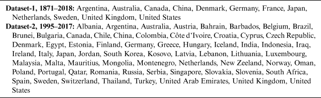
As mentioned earlier, we employ two datasets for the assessment of the relationship between fine wine imports and income inequality. Dataset 1 covers wine import value, income inequality, and per capita GDP data for the 12 largest wine importers worldwide between 1871 and 2018 (WID, 2019). Dataset 1 estimates account for Prohibition in the United States from 1920 to 1933, Canada from 1918 to 1920, Norway from 1916 to 1927, and Russia from 1914 to 1925, by treating the observations for these years as missing values. Dataset 2 concerns wine imports from France and includes wine imports and income inequalities for 66 countries for the years 1995 to 2017 (WID, 2019; WDI, 2019) (Table 1). Data on wine imports in Dataset 1 is sourced from the UN Comtrade Database (2018). Data on the value of French wine exports is sourced from Eurostat (2018). The countries with full alcohol import bans have been eliminated from the Dataset 2.
List of Countries Dataset-1&2

The rationale behind employing two datasets are not just the robustness of the estimates, because these kind of robustness checks were not fully congruent due to the diverging time intervals and different countries in the respective datasets. The central merit of Dataset 1 is the large T, which yields more efficient estimators than the shorter series. The major advantage of Dataset 2 is the inclusion of French wine imports, which epitomize luxury and status more than wines from other countries (Pan, Fang, and Malaga, Reference Pan, Fang and Malaga2006; Corsi, Reference Corsi2016). The increasing import volume in the case of Dataset 1, which includes total imports, could be biased as a result of increasing import demand due to low-import prices rather than solely due to the luxury value. In Dataset 2, the variation in the import quantity of relatively expensive French fine wines could also be partly attributed to the increasing prices for domestic fine wines, but definitely to a much lesser degree than in Dataset 1, which contemplates the total fine wine imports.
The main limitation of the study relates to the wine import data. These data do not differentiate between the prices of imported wines, leading to the aggregation of luxury, super-luxury, icon, dream, and non-luxury wines in the aggregated import data (Cholette and Castaldi, Reference Cholette and Castaldi2005; Jarrett and Jarvis, Reference Jarrett, Jarvis and Bruwer2016).
IV. Results and Discussion
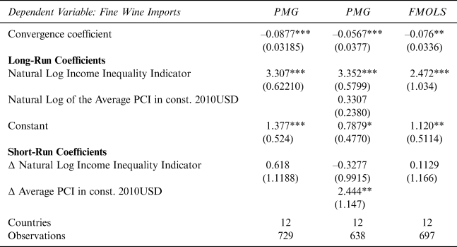
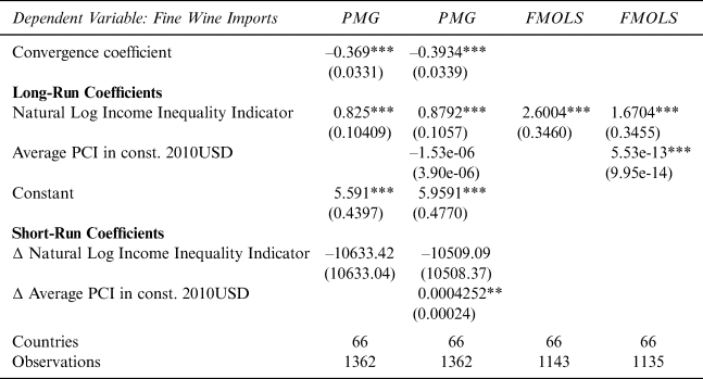
The PMG and FMOLS estimates (see Tables 2 and 3) for both datasets reveal a statistically significant and robust positive long-run relationship between income inequality and the volume of fine wine imports, with the elasticities based on Dataset 1 being between 2.472 and 3.307 percent. The estimations with Dataset 2, on the other hand, are between 0.825 and 2.6004 percent. Changing income inequality has no short-run effect on the volume of fine wine imports in either dataset. PCI, in contrast, has only a short-run statistically significant impact on the volume of fine wine imports whereby the corresponding elasticities range between 0.004 and 2.444 percent.
Panel Estimates for Dataset 1 (1871–2018)

Note: The asterisks *,**, and *** indicate P values of 0.1, 0.05, and 0.01, respectively.
Source: Authors’ own calculations.
Panel Estimates for Dataset 2 (1995–2017)

Note: The asterisks *,**, and *** indicate P values of 0.1, 0.05, and 0.01, respectively.
Source: Authors’ own calculations.
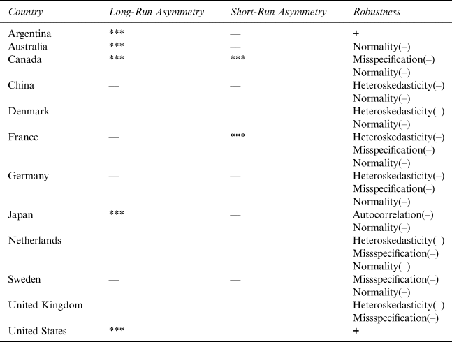
To address the issue of (a)symmetry, we employed the country-specific NARDL estimators for 12 countries from Dataset 1.Footnote 1 The estimates summarized in Table 4 reveal a mixed picture. We detect the robust long-run asymmetry only for Argentina and the United States. These findings indicate that, at least in these countries, path dependency exists, whereby wine imports increase because of increasing inequality, but show persistence if inequality decreases. One possible explanation for this phenomenon could be the absorption of imported fine wines by the taste culture of the respective countries (Harding, Reference Harding2017). The reasons for this kind of persistence are, however, beyond the scope of this investigation and will be addressed in follow up surveys.Footnote 2
NARDL-Asymmetry Assessment Results

Notes: The asterisks *,**, and *** indicate P values of 0.1, 0.05, and 0.01, respectively. “+” means that all three tests indicate the robustness of the result; “–” in front of the test indicates that the test was not successful.
Source: Authors’ own calculations.