





1. Introduction
Internal waves are oscillatory motions driven by buoyancy forces in a stably stratified fluid. They play a central role in ocean dynamics by transporting energy both horizontally and vertically, and by driving turbulent mixing when they break (Polzin et al. Reference Polzin, Toole, Ledwell and Schmitt1997; Ferrari & Wunsch Reference Ferrari and Wunsch2009; Roemmich et al. Reference Roemmich, Church, Gilson, Monselesan, Sutton and Wijffels2015). Besides their surface generation by winds, an important source of the waves is the motion of the barotropic tide over submarine topography, notably near islands, trenches and mid-ocean ridges (Ray & Mitchum Reference Ray and Mitchum1996; Egbert & Ray Reference Egbert and Ray2000). This oscillatory flow over sufficiently steep topography launches internal tides, which are horizontally and vertically propagating beams of internal waves with the frequency of the tidal forcing (Balmforth et al. Reference Balmforth, Ierley and Young2002). These internal tides carry energy away from the generation site toward the ocean surface (Martin et al. Reference Martin, Rudnick and Pinkel2006).
Field observations have been instrumental in revealing the fate of tidally generated internal tide energy. Measurements near major topographic features, such as the Hawaiian Ridge (Rudnick et al. Reference Rudnick2003) and Luzon Strait (Alford et al. Reference Alford2011), show that, while some internal tide energy dissipates locally, a substantial fraction radiates into the far field as low-mode internal tides. Satellite altimetry and island tide gauges detect coherent sea-surface height anomalies – typically a few centimetres in amplitude – propagating more than 1000 km from their generation sites (Ray & Mitchum Reference Ray and Mitchum1997). Acoustic tomography experiments similarly reveal coherent internal tides that have travelled over 2000 km northward from the Hawaiian Ridge (Dushaw et al. Reference Dushaw, Howe, Cornuelle, Worcester and Luther1995; Kantha & Tierney Reference Kantha and Tierney1997; Egbert & Ray Reference Egbert and Ray2000; Rainville & Pinkel Reference Rainville and Pinkel2006b ).
In situ measurements near Hawaii show that the energy flux is dominated by the semidiurnal (
 $M_2$
) tide and varies with the spring–neap cycle. While energetic beams are observed near the ridge, the energy flux 450 km offshore is carried primarily by the first baroclinic mode, indicating that much of the higher-mode energy dissipates near the generation region (Rainville & Pinkel Reference Rainville and Pinkel2006b
). The Luzon Strait likewise produces some of the largest internal waves in the ocean, which radiate westward into the South China Sea. The propagation of these waves is further influenced by mesoscale eddies, which can refract wave beams and randomise their phase, particularly for higher modes (Rainville & Pinkel Reference Rainville and Pinkel2006a
). Notably, field measurements near generation sites consistently show enhanced turbulent dissipation close to the ocean surface where upward-propagating beams are expected to reflect. It is unclear in the observations whether or not the incident beams in fact reflect from the near-surface region (Martin et al. Reference Martin, Rudnick and Pinkel2006; Cole et al. Reference Cole, Rudnick, Hodges and Martin2009).
In parallel, a large body of theoretical, numerical and laboratory work has explored the physics of internal wave generation and propagation. Experiments and simulations also show that, even with large tidal excursions that introduce nonlinear effects, the energy conversion into the dominant mode-1 tide remains robust (Echeverri et al. Reference Echeverri, Flynn, Winters and Peacock2009). Echeverri et al. (Reference Echeverri, Yokossi, Balmforth and Peacock2011) showed that complex topographies, such as double-ridge systems, can trap waves, causing them to reflect repeatedly and focus energy into distinct geometrical structures. It has been shown that the interaction with boundaries is often nonlinear, acting as a source for higher-harmonic disturbances that radiate away as new wave beams (Tabaei et al. Reference Tabaei, Akylas and Lamb2005). Laboratory experiments have confirmed that, when an internal wave beam is incident on a pycnocline in the absence of shear, a discrete spectrum of higher-frequency modes is generated due to nonlinear effects (Wunsch & Brandt Reference Wunsch and Brandt2012). Numerical simulations further show that an incident wave beam can undergo parametric subharmonic instability, a nonlinear process in which the large-scale internal wave transfers its energy to two smaller-scale waves. During the interaction of the wave beam with the model pycnocline, it is refracted, leading to the formation of waves which finally break down into turbulence (Gayen & Sarkar Reference Gayen and Sarkar2014). This instability and subsequent turbulent breakdown can substantially weaken the reflected wave beam, with simulations showing that only approximately 30
 $\%$
of the incoming energy is transported by the main reflected beam after the interaction (Gayen & Sarkar Reference Gayen and Sarkar2014).
While the numerical simulations and laboratory experiments discussed above suggest that upward-propagating internal tide beams reflect all or in part from the surface/pycnocline, the presence of reflected beams in field measurements is less clear. This suggests that additional physical processes, potentially associated with near-surface turbulence, may influence wave reflection in ways not captured by idealised models. Examining aspects of near surface turbulence influence upon wave reflection/absorption is the central motivation for the present study. Specifically, this work, for the first time, investigates the dynamics of internal wave beams interacting with an explicitly simulated layer of idealised stratified turbulence. Our approach utilises direct numerical simulations (DNS), which allows us to resolve the full range of turbulent scales and precisely control the properties of both the incoming wave and the turbulent layer. This methodology enables a systematic examination of how an idealised stratified turbulent layer modulates wave reflection, transmission and dissipation, and how these processes depend on key parameters such as wave frequency and amplitude. We will show that, in our simulations, the stratified turbulent layer can act as a highly efficient sink for incident internal wave energy, particularly for lower-frequency waves within the range explored here. This absorption of energy can significantly alter the reflection process, leading to a significant suppression of the reflected wave beam and suggesting a possible mechanism that may contribute to discrepancies between idealised models and oceanic observations.
The remainder of this paper is structured as follows. In § 2, we describe the numerical set-up, including the governing equations and the methods used to generate both the stratified turbulence and the incident wave beams. In § 3, we present our results, beginning with detailed analyses of two simulations, one with no wave forcing and the other with a wave forced at a particular frequency. We go on to explore how the wave–turbulence interaction depends on wave frequency and amplitude, culminating in measurements of the reflection coefficient. Finally, we discuss the implications of our findings and present our conclusions in § 4.
2. Numerical model
We use three-dimensional DNS to model internal waves impinging upon a layer of stratified turbulence in a Boussinesq fluid. The initial background stratification is uniform throughout the domain, characterised by a constant buoyancy frequency
 $N_0=[-(g/\rho _0)\,{\rm d}\bar {\rho }/{\rm d}z]^{1/2}$
, in which
 $g$
is gravity,
 $\rho _0$
is the characteristic density and
 $\bar {\rho }$
is the background density which decreases linearly with height,
 $z$
. The incident waves are spanwise-uniform in the
 $y$
-direction and horizontally periodic with one wavelength spanning the domain in the
 $x$
-direction. As discussed below, numerical constraints prevent us from examining very low-frequency waves that are influenced by the Earth’s rotation. For this reason, our equations do not include Coriolis forces. However, the results of our simulations, spanning non-hydrostatic to hydrostatic incident waves, may provide qualitative insight into the behaviour of the lower-frequency internal wave dynamics.
Although most results presented here are given in dimensional form, in practice the numerical model works with non-dimensional variables, scaling time by
 $N_0^{-1}$
and scaling length by
 $k_0^{-1}$
, in which
 $k_0=2\pi /\lambda$
is the horizontal wavenumber of the incident waves with wavelength
 $\lambda$
. The domain itself measures
 $L=2\pi /k_0$
on each side. The vertical coordinate ranges between
 $-L/2$
and
 $L/2$
, with stratified turbulence being forced in the upper half of the domain,
 $0\lesssim z\leqslant L/2$
. Upward-propagating waves are forced near the centre of the bottom half of the domain, and damping is included near the bottom of the domain to prevent downward-propagating waves from reflecting back upward. A sketch of the set-up of the numerical simulations is shown in figure 1.
(a) Schematic of the set-up of the simulation domain. The pink region indicates the forced turbulent layer in the top half of the domain, the blue region indicates where upward-propagating waves are forced and the grey region indicates where downward-propagating disturbances are damped. (b) Vertical structure of the turbulence forcing,
 $\mathcal{H}_T$
(pink), and wave forcing,
 $\mathcal{H}_{\mathcal{W}}$
(blue).

Figure 1. Long description
Panel A: The schematic shows a vertical cross-section of a simulation domain. The top half of the domain is shaded pink and labeled as the forced turbulent layer, where turbulence forcing is applied. The middle section is shaded blue and indicates where upward-propagating waves are forced. The bottom section is shaded grey and represents a sponge layer where downward-propagating disturbances are damped. The z-axis is vertical, with labels indicating different layers at specific depths. Panel B: The graph shows the vertical structure of turbulence forcing in pink and wave forcing in blue. The vertical axis is labeled ‘z’ and ranges from -L/2 to L/2. The horizontal axis is labeled ‘Amplitude’ and ranges from 0 to 1. The pink curve represents the amplitude of turbulence forcing, which decreases from the top (z = L/2) to the middle (z = 0). The blue curve represents the amplitude of wave forcing, which increases from the middle (z = 0) to the bottom (z = -L/2).
2.1. Model equations
The non-dimensional Boussinesq momentum, buoyancy and continuity equations for an incompressible fluid are
 \begin{align} \frac {\mathrm{D}{\tilde {u}}}{\mathrm{D}\tilde {t}} = -\boldsymbol{\nabla }\tilde {P} + \tilde {b}\,\hat {\boldsymbol{z}} + \frac {1}{{{Re}}} \tilde {{\nabla} }^2 {\tilde {u}} + \mathcal{F}_{{T}} + \mathcal{F}_{\textit{W}{{u}}} + \mathcal{D}\,{\tilde {u}}, \end{align}
 \begin{align} \frac {\mathrm{D} \tilde {b}}{\mathrm{D}\tilde {t}} = -\tilde {w} + \frac {1}{{{Re}}\,{{Pr}}} \tilde {{\nabla} }^2 \tilde {b} +\mathcal{F}_{\textit{W}b} + \mathcal{D}\,\tilde {b}, \end{align}
 \begin{align} \tilde {\boldsymbol{\nabla }} \boldsymbol{\cdot }{\tilde {u}} = 0, \end{align}
in which
 ${\tilde {u}}={u}\,k_0/N_0$
,
 $\tilde {b}=b\,k_0/N_0^2$
and
 $\tilde {P}=P\,k_0^2/N_0^2$
. In dimensional form,
 $\mathrm{D}/\mathrm{D}t = \partial /\partial t\ +\ {u}\boldsymbol{\cdot }\boldsymbol{\nabla}$
is the material derivative,
 ${u}$
is velocity with components
 $u$
,
 $v$
and
 $w$
respectively in the
 $x$
,
 $y$
and
 $z$
directions,
 $P$
is the density-scaled fluctuation pressure and
 $b$
is the fluctuation buoyancy field (given dimensionally by
 $-g\rho /\rho _0$
, in which
 $\rho$
is the fluctuation density). The buoyancy force acts only in the
 $z$
-direction, denoted by
 $\hat {\boldsymbol{z}}$
. Momentum diffusion is quantified by the Reynolds number,
 ${{Re}} \equiv N_0\,k_0^{-2}/\nu$
, in which
 $\nu$
is the kinematic viscosity. Throughout, we take
 ${{Re}}=10^4$
. Likewise the magnitude of the diffusion of buoyancy relative to momentum diffusivity is given by the Prandtl number,
 ${ {Pr}} \equiv \nu /\kappa$
. Physically,
 $\kappa$
could represent the diffusivity of heat (
 ${ {Pr}}=7$
) or salt (
 ${ {Pr}}=700$
). However, to avoid high computational costs associated with resolving the fine turbulent scales of the buoyancy field at high Prandtl numbers, we take
 ${ {Pr}}=1$
. The remaining terms in (2.1) and (2.2) represent explicit forcing of turbulence (
 ${\mathcal F}_{\text{T}}$
) and waves (
 ${\mathcal F}_{\textit{W}{{u}}}$
and
 ${\mathcal F}_{\textit{W}{b}}$
), as well as explicit damping terms (
 ${\mathcal D}\,{u}$
and
 ${\mathcal D}\,b$
). We next describe each of these terms in detail.
The divergence-free forcing of the turbulent region follows the approach of Maffioli (Reference Maffioli2017), in which only the horizontal flow is forced by horizontally sinusoidal disturbances with uniform vertical structure. Explicitly, at each time the
 $x$
-,
 $y$
-,
 $z$
-components of the forcing are given by
 \begin{align} {\mathcal F}_{\text{T}} = (\sin \varphi (t),\,-\cos \varphi (t),\,0)\, F_T(t)\,{\mathcal H}_{\text{T}}(z)\,\cos [{k}_h(t)\boldsymbol{\cdot }{x}_h + \phi (t)], \end{align}
in which
 $\boldsymbol{k}_h = k_{f0} (\cos \varphi (t),\ \sin \varphi (t))$
is the horizontal wavenumber vector of the forcing with
 $\varphi (t)$
being its direction and
 $k_{f0}$
its magnitude. The orientation of the horizontal component of the forcing ensures
 $\boldsymbol{\nabla }\boldsymbol{\cdot }{\mathcal F}_{\text{T}} = \boldsymbol{k}_h\boldsymbol{\cdot }{\mathcal F}_{\text{T}}= 0$
. The horizontal wavenumbers
 $(k_x, k_y)$
were chosen such that the total magnitude
 $k_h = \sqrt {k_x^2 + k_y^2}$
satisfied
 $k_{f,\textit{min}} \lt k_h \lt k_{f,\textit{max} }$
, with
 $k_f = 6k_0$
defining the characteristic forcing scale. Thus horizontal motion is forced as scales approximately 6 times smaller than the scale of the incident wave. Each allowed mode was assigned a random phase uniformly distributed in
 $[0, 2\pi )$
, and the forcing vector was constructed to be divergence free by setting
 $ \hat {f}_x({k}) \propto ({k_y}/{k_h}) \cos \phi , \hat {f}_y({k}) \propto -({k_x}/{k_h}) \cos \phi$
, where
 $\phi$
denotes the random phase. This ensures that
 $\boldsymbol{\nabla }\boldsymbol{\cdot }{f} = 0$
and the forcing does not directly inject compressible motions. The forcing amplitude,
 $F_T(t)$
, also varies in time. Its value is chosen to ensure the input power due to forcing remains constant (see Maffioli Reference Maffioli2017). In all our simulations we set this power to be
 $1.5N_0^3/k_0^2$
, chosen to be large enough to trigger sustained turbulence while maintaining adequate numerical resolution of the smallest scales. Unlike Maffioli (Reference Maffioli2017), we force stratified turbulence only in the top half of our domain. Hence, we define the smooth change in forcing amplitude with the vertical by
 \begin{align} {\mathcal H}_{{T}}(z)= (1+\tanh (z/\sigma _t))/2, \end{align}
which transitions from
 $0$
in the bottom of the domain to
 $1$
in the top of the domain over a distance
 $\sigma _t$
about
 $z=0$
. In all simulations we chose
 $\sigma _t=0.25k_0^{-1}$
to be small enough to separate the turbulent-forced region from the wave-forced region, and large enough to avoid a sharp turbulent/non-turbulent interface which would strongly excite internal waves below the turbulent region (figure 1).
The incident upward-propagating waves are forced near the centre of the bottom half of the domain. The buoyancy forcing is given by
 \begin{align} {\mathcal F}_{\textit{W}b} = A_{\dot {b}}\,F_W(t)\,{\mathcal H}_{\textit{W}}(z)\, \cos (k_0 x -\omega _0 t). \end{align}
We run simulations with different wave-forcing frequencies,
 $\omega _0$
, and amplitudes,
 $A_{\dot {b}}$
, as listed in table 1. In particular, we investigate frequencies ranging from
 $0.1N_0$
(hydrostatic waves) to
 $0.6N_0$
(non-hydrostatic waves). From the dispersion relation for internal waves, the corresponding vertical wavenumber of the forced waves is
 \begin{align} k_{z0} = - k_0 (N_0^2/\omega _0^2 -1)^{1/2}. \end{align}
Parameters for simulations of forced wave incident upon stratified turbulence, and results showing the forcing amplitude (
 $A_{\dot {b}}$
) and frequency (
 $\omega _0$
), the predicted amplitude of the buoyancy field compared with the critical amplitude (
 $A_{b0}/A_{bc}$
), the predicted amplitudes of the horizontal (
 $A_{u0}$
) and vertical (
 $A_{w0}$
) velocities and the measured reflection coefficient,
 $\mathcal{R}$
, given by (3.1). The case
 $\mathcal{R}\gt 1$
corresponds to waves that are over-reflected. For completeness, we also list the simulation ‘TURB-NW’ with no wave forcing.

Table 1. Long description
A table with 7 rows and 8 columns comparing simulation parameters and results for forced wave incident upon stratified turbulence. The columns are Simulation ID, A b 0 divided by (N 0 cubed divided by k 0), omega 0 divided by N 0, A b 0 divided by A b c, A u 0 divided by (N 0 divided by k 0), A u 0 divided by (N 0 divided by k 0), and R. The rows are TURB-W1, TURB-W2, TURB-W3, TURB-W4, TURB-W5, TURB-W6, and TURB-NW. Each row lists specific values for the parameters and results of the simulations.
This is set to be negative to correspond to waves with upward group velocity (Sutherland Reference Sutherland2010). In our simulations the magnitude of the vertical wavenumber ranges from
 $\simeq 9.9k_0$
(for
 $\omega _0=0.1N_0$
) to
 $1.3k_0$
(for
 $\omega _0=0.6N_0$
).
As with the turbulence forcing, the magnitude of the wave forcing is also a function of
 $z$
and
 $t$
. In the vertical, the spatial structure is given by
 \begin{align} {\mathcal H}_{\textit{W}}(z)=\exp \big [-(z-z_w)^2/(2\sigma _w^2)\big ], \end{align}
where the centre of the forcing region is at
 $z_w\simeq -1.64k_0^{-1}$
with the amplitude falling off as a Gaussian with standard deviation
 $\sigma _w=0.25k_0^{-1}$
. After a delay of time
 $T_d$
, the forcing is increased over a wave period,
 $T_0=2\pi /\omega _0$
, from zero to forcing at constant amplitude. This gradual ramp-up of the forcing avoids sudden changes that would excite high-frequency disturbances. The forcing is expressed by
 \begin{align} F_W(t) = \frac {1}{2} \left [1 + \tanh \left (\frac {t-T_d-T_0}{T_0}\right )\right ], \end{align}
which smoothly transitions from near
 $0$
at the start of the simulations to
 $1$
at late times. Typically, we take
 $T_d=T_0$
.
After a time when the forcing becomes constant (
 $t/T_0\gg 1+T_d/T_0$
), the amplitude of the resulting waves is predicted by time integrating the forcing acting on the wave as it moves across the forcing region at the vertical group velocity. As shown in Appendix A, the steady-state amplitude of the buoyancy field given in terms of the forcing amplitude,
 $A_{\dot {b}}$
, is predicted to be
 \begin{align} A_{b0} = \sqrt {2\pi }\,\frac {k_0\sigma _w}{N_0}\,(\sin \varTheta \,\cos ^2\varTheta )^{-1} A_{\dot {b}}, \end{align}
in which
 $\varTheta \equiv \cos ^{-1}(\omega _0/N_0)$
. In most simulations, we set the amplitude of the wave forcing of buoyancy to be
 $A_{\dot {b}}=0.004 N_0^3/k_0$
. This is chosen to be sufficiently large for the signal of waves to be detectable over other disturbances occurring in the simulations, but not so large that the waves are overturning, i.e.
 $\partial _z b \lt -N_0^2$
somewhere in the wave field. Explicitly, waves are overturning if
 $A_{b0} \gt A_{bc} \equiv (N_0^2/k_0) \cot \varTheta$
(Sutherland Reference Sutherland2010). In our simulations with
 $A_{\dot {b}}=0.004N_0^3/k_0$
,
 $A_{b0}/A_{bc}$
ranges from
 $\simeq 0.3$
(with
 $\omega _0=0.2N_0$
) to
 $0.012$
(with
 $\omega _0=0.6N_0$
). We also perform simulations with smaller-amplitude forcing,
 $A_{\dot {b}}=0.001N_0^3/k_0$
, of low-frequency waves with
 $\omega _0=0.1N_0$
and
 $0.2N_0$
, for which
 $A_{b0}/A_{bc} \simeq 0.6$
and
 $0.08$
, respectively.
The wave forcing of the vertical velocity follows from the polarisation relations for internal waves
 \begin{align} {\mathcal F}_{\textit{W}w} = -\frac {\cos \varTheta }{N_0} A_{\dot {b}}\ F_W(t){\mathcal H}_{\textit{W}}(z)\ \sin (k_0 x -\omega _0 t). \end{align}
The forcing of the horizontal velocity in the
 $x$
-direction is
 \begin{align} {\mathcal F}_{\textit{W}u} = -\frac {\sin \varTheta }{N_0} A_{\dot {b}}\ F_W(t){\mathcal H}_{\textit{W}}(z)\ \sin (k_0 x -\omega _0 t) + A_0\ F_W^2(t) {\mathcal H}_{\textit{W}0}(z). \end{align}
The first term follows from the polarisation relations. The second term is a mean-flow forcing which counteracts the deceleration of the flow in the forcing region due to the extraction of momentum from this region by the forced waves. The derivation of the amplitude and vertical structure of the forcing is given in Appendix A. Explicitly, we show that
 \begin{align} A_0 = \frac {\sqrt {\pi }}{2} A_{\dot {b}}^2 \frac {k_0^2\sigma _w}{N_0^4}\ (\sin \varTheta \,\cos ^3\varTheta )^{-1} \end{align}
and
 \begin{align} {\mathcal H}_{\textit{W}0}(z) = \left [1 + {\textrm {erf}}\left (\frac {z-z_w}{\sqrt {2}\sigma _w}\right )\right ] \exp \left (-\frac {(z-z_w)^2}{2\sigma _w^2}\right ) \, . \end{align}
There is no forcing of the horizontal velocity in the
 $y$
-direction.
Although we force internal waves to propagate upward toward the base of the turbulent layer, we will show that the stratified turbulence itself launches downward-propagating waves. To prevent these waves, and other downward-propagating disturbances, from reflecting off the bottom of the domain, we introduce a Rayleigh damping operator,
 $\mathcal{D}$
, which is applied to both buoyancy and velocity fields. The strength of the damping in the vertical is adopted from Slinn & Riley (Reference Slinn and Riley1998) as
 \begin{align} \mathcal{D} = \exp \big (-\frac {(z-z_d)^2}{2\sigma _d^2}\big ). \end{align}
The peak of the damping occurs at
 $z_d\simeq -2.4k_0^{-1}$
and falls off over a distance
 $\sigma _d\simeq 0.2k_0^{-1}$
.
We note that the forcing amplitudes in table 1 are not intended to quantitatively match the oceanographic condition. Instead, they are chosen to ensure that both the wave field and the turbulence motions are sufficiently energetic and resolved within the limits of DNS. Nevertheless, this configuration allows us to resolve both the wave field and turbulent motions simultaneously, allowing us to examine the wave–turbulence interactions that would be difficult to isolate in more realistic parameter regimes.
2.2. Numerical set-up
The simulations are carried out using Dedalus, a flexible framework for solving partial differential equations using spectral methods (Burns et al. Reference Burns, Vasil, Oishi, Lecoanet and Brown2020). The cubic domain has periodic boundary conditions in the horizontal and free-slip conditions at the top and bottom boundaries. Since the flow is assumed to be incompressible, we impose a gauge condition to ensure uniqueness,
 $ \int _V p \, {\rm d}V = 0,$
, where
 $V$
denotes the computational domain. In all simulations that we present in this study, the equations of motion are discretised by Fourier series with
 $N_x=N_y=512$
modes in the horizontal and by Chebyshev polynomials with
 $N_z=512$
modes in the vertical. The resolution is chosen to ensure that the smallest scales of turbulence are adequately resolved, as described below.
Fields are advanced in time using second-order backward differentiation, which is an implicit–explicit time-stepping scheme chosen for its stability and accuracy (Wang & Ruuth Reference Wang and Ruuth2008). Although simulations begin with a time step of
 $\simeq 1.57N_0^{-1}$
this is reduced as the flow evolves to ensure that the Courant–Friedrichs–Lewy (CFL) condition is satisfied with a safety factor of
 $0.2$
. Specifically, we calculate the CFL estimate of the time-step size to be
 $\Delta t = 0.2 \max ({|u|}/{\Delta x}) + ({|v|}/{\Delta y}) + ({|w|}/{\Delta z} )^{-1},$
where the maximum is taken over the quadrature grid points. This estimate is calculated on each time step, but we only change the time-step size compared with the previous time step if the estimate differs from the previous time-step size by greater than 5 %.
Simulations are run for sufficiently long time to allow stratified turbulence to develop and then have forced waves interact with the turbulence over a time of at least 6 wave periods up to times above
 $t=450N_0^{-1}$
(
 $\simeq 70$
buoyancy periods). A single simulation running in parallel on 1536 cores took 72 hours (
 $\approx 1.1\times 10^{5}$
core-hours) to complete. Because of the computational expense of these simulations, we limit our study to focus on waves forced at frequencies of
 $0.1N_0$
and higher. Lower-frequency waves take longer to develop and propagate toward the stratified layer, meaning that, as the forcing frequency is decreased, simulations would need to be run for longer times to capture the steady-state dynamics over many wave periods.
2.3. Diagnostics
To assess how well the simulations resolve motion in the stratified turbulent region, we periodically compute vertical profiles of the horizontally averaged kinetic energy
 \begin{align} \mathcal{K}(z) \equiv \frac {1}{2} \langle |{u}|^2\rangle \end{align}
and the horizontally averaged kinetic energy dissipation rate and viscosity times the horizontally averaged enstrophy given respectively in non-dimensional form by
 \begin{align} \widetilde{\mathcal{E}}(z) \equiv \langle \tilde {\epsilon }\rangle \equiv \frac {2}{{{Re}}} \langle \tilde {D}_{ij}\tilde {D}_{ij}\rangle ,\quad \widetilde {\mathcal{Z}}(z) \equiv \frac {1}{{{Re}}} \langle |\tilde {\boldsymbol{\nabla }}\times {\tilde {u}}|^2 \rangle , \end{align}
in which
 $\tilde {D}_{ij}=(\partial \tilde {u}_i/\partial \tilde {x}_j + \partial \tilde {u}_j/\partial \tilde {x}_i)/2$
are the components of the deformation tensor and summation takes place over indices
 $i$
and
 $j$
. The angled brackets indicate a horizontal average taken over the full domain. As anticipated, we find there is negligible difference between
 $\widetilde {\mathcal{E}}$
and
 $\widetilde {\mathcal{Z}}$
(Yeung et al. Reference Yeung, Donzis and Sreenivasan2012). Thus, we estimate the energy dissipation rate by calculating the less computationally expensive diagnostic,
 $\widetilde {\mathcal{Z}}$
, which is saved every
 $0.1\,N_0^{-1}$
time units.
We assess how well the simulations resolve turbulent scales by comparing the grid resolution with the predicted Kolmogorov scale (i.e. the scale at which we expect motions to be damped by viscosity). In dimensional units, this quantity is given by
 $(\nu ^3/{\mathcal{Z}}^\star )^{1/4}$
. Non-dimensionally, the Kolmogorov scale is estimated by
 \begin{align} L_k = ({{Re}}^{-3}/\widetilde {\mathcal{Z}})^{1/4}. \end{align}
We compare this scale with the vertical resolution in simulations,
 $\Delta$
, which varies in the vertical and is largest about
 $z=0$
due to the use of Chebyshev polynomials in the vertical. We typically find peak values of the ratio
 $\Delta /L_K$
occur in the range
 $0.1\leqslant z/L\leqslant 0.4$
for which, on average,
 $\langle \Delta /L_k\rangle \sim 2.9\pm 0.1$
. This indicates that the dissipative scales are marginally resolved (see, for example, discussions of resolution requirements in other stratified turbulent flows in Smyth & Moum Reference Smyth and Moum2000; Kaminski & Smyth Reference Kaminski and Smyth2019).
We also compute the buoyancy Reynolds number, defined in terms of enstrophy by
 ${\mathcal{Z}}/(\nu N_0^2)$
. Non-dimensionally it is
 \begin{align} {Re}_b = \widetilde {\mathcal{Z}}\,{{Re}} \end{align}.
The buoyancy Reynolds number can also be written as
 ${Re}_b=(L_o/L_k)^{4/3}$
, in which
 $L_o\simeq ({\mathcal{Z}}/N_0^3)^{1/2}$
is the Ozmidov scale, which is a measure of the largest vertical scale that is not influenced by stratification. Typically, we find
 ${Re}_b\simeq 6 \pm 1$
, indicating a limited range of scales over which dissipation is not influenced by buoyancy. We note that, if our study here focused on mixing efficiency, it would have been better to have
 $\langle \Delta /L_k\rangle \lesssim 2$
(Gregg. et al. Reference Gregg., D’Asaro, Riley and Kunze2018) and
 ${Re}_b\gtrsim 10$
(Bartello & Tobias Reference Bartello and Tobias2013). However, in the simulations here the resolution is sufficient to capture the process of large-scale incident waves interacting with structures in the inertial range of turbulence. The relatively modest value
 ${Re}_b\simeq 6$
indicates limited scale separation between buoyancy-affected motions and dissipative scales. Thus, the turbulent layer in our simulations should not be interpreted as representative of fully developed oceanic mixed-layer turbulence. Instead, it provides an idealised stratified turbulent region in which wave–turbulence interactions can be isolated under controlled DNS conditions.
Even in the absence of wave forcing, the base of the stratified region excites downward-propagating internal waves, which are ultimately damped near the bottom of the domain. Although their horizontal wavenumber is generally larger than
 $k_0=1$
, their amplitude can be comparable to and even larger than that of the forced waves. In order to study the upward propagation and possible reflection and dissipation of the forced waves, in post-processing we first use dynamic mode decomposition (Schmid Reference Schmid2022) to extract structures with the frequency
 $\omega _0$
of the forced waves and then use Hilbert transforms to separate upward- from downward-propagating signals (Mercier et al. Reference Mercier, Garnier and Dauxois2008).
To apply dynamic mode decomposition (hereafter, DMD), we first extract vertical slices of
 $u$
,
 $w$
and
 $b$
at integer non-dimensional times,
 $N_0t$
, beginning when the stratified turbulence and wave forcing are fully developed and the system is in quasi-steady state. Typically, these slices are extracted between times
 $150N_0^{-1}$
and
 $450N_0^{-1}$
. We examine slices extracted from the plane
 $y=0$
. The DMD analysis takes these spatio-temporal fields and returns the best-correlated structures associated with different frequencies. From this we extract the structure of the horizontal velocity field with frequency
 $\omega _0$
. This complex-valued field has real part corresponding to the structure at zero phase of the disturbance and an imaginary part representing the structure a quarter period later.
The Hilbert transform involves taking a Fourier transform in the vertical and then filtering for positive and negative vertical wavenumber components. Because our domain is not vertically periodic, taking Fourier transforms would cause aliasing errors associated with sharp changes between the bottom of the non-turbulent layer and the top of the turbulent layer. To avoid aliasing errors we first take the fields produced by the DMD analysis and reflect them in the vertical to create fields spanning twice the domain height, which smoothly change from the original non-turbulent lower region to the stratified turbulent layer, to the reflected stratified turbulent layer to the reflected non-turbulent layer. The vertically reflected complex-valued DMD field for a particular frequency is then Fourier transformed in the vertical. To extract upward-propagating waves (with positive vertical group velocity), we keep only the Fourier components with
 $k_z\lt 0$
. The result is then inverse transformed and (spatial) values corresponding to the original domain height are extracted. Likewise we extract downward-propagating waves by keeping only the Fourier components with
 $k_z\gt 0$
.
When internal waves dissipate, they deposit horizontal momentum to the background flow field as a consequence of the divergence of their vertical flux of horizontal momentum. The horizontal spectrum of downward-propagating internal waves generated by turbulence is isotropic, and so should have negligible net impact on the mean flow. Inversely, the forced waves are generated with positive momentum flux, and are therefore expected to contribute to a rightward acceleration of the mean flow as they dissipate. To examine the impact of the forced waves upon the mean flow, at each integer time from the simulations we extract snapshots of
 $u$
from four vertical planes at
 $y=-L/2$
,
 $-L/4$
,
 $0$
and
 $L/4$
. Each are averaged in
 $x$
and the resulting four vertical profiles are averaged together (we denote this averaging procedure by an overline). The successive vertical profiles are then stacked in time to construct a vertical time series of
 $\bar {u}(z,t)$
.
3. Results
In this section we begin by showing the results of simulations in which the turbulence is forced in the upper half of the domain, but there is no explicit wave forcing from below. Thereafter we present the results of simulations with explicit wave forcing.
3.1. Results from simulations with no wave forcing
Figure 2 shows snapshots from a simulation with no wave forcing in which the columnar forcing of the horizontal velocity in the upper layer produces stratified turbulence. At
 $t=50N_0^{-1}$
the columnar forcing of the horizontal velocity in the upper layer begins to break down, with finer structures developing just above
 $z=0$
(figure 2
a). At the same time,
 $b$
exhibits fine-scale perturbations above
 $z=0$
as well as relatively larger-scale disturbances in the unforced region below
 $z=0$
(figure 2
d). This is consistent with the generation of downward-propagating internal waves by developing turbulence, as evidenced by the larger-scale disturbances observed below
 $z=0$
. At later times
 $u$
and
 $b$
exhibit a wider range of scales above
 $z=0$
(figure 2
b,e). As expected for stratified turbulence, the horizontal velocity is anisotropic (Caulfield Reference Caulfield2021), exhibiting longer coherence in the horizontal than vertical (figure 2
b,c). Below
 $z=0$
, the disturbances associated with downward-propagating excited internal waves have smaller horizontal and vertical scales than at
 $t=50N_0^{-1}$
, although their spectrum is visibly narrower than that in the turbulent region. Figure 2(f), shows the local kinetic energy dissipation rate,
 $\epsilon$
. This shows that dissipation occurs most significantly in the upper half of the domain where it is turbulent. Regions of large dissipation are localised and patchy, as expected for stratified turbulence (Garaud et al. Reference Garaud, Chini, Cope, Shah and Caulfield2024).
From a simulation without wave forcing, snapshots at times (a,d)
 $N_0t=50$
and (b,c,e,f)
 $N_0t=200$
showing (a,b) the
 $x$
-component of velocity,
 $u$
, at in the
 $y=0$
plane, (d,e) buoyancy fluctuations
 $b$
in the
 $y=0$
plane, (c) the
 $y$
-component of velocity,
 $v$
, in the
 $x=0$
plane and (f) the dissipation rate
 $\epsilon$
in the
 $y=0$
plane. The colour scale for
 $\tilde {u}=u\,k_0/N_0$
in (b) is indicted in (a); the colour scale for
 $\tilde {b}=b\,k_0/N_0^2$
in (e) is indicated in (d).

The development of turbulent kinetic energy (see (2.16)) and dissipation (see (2.17)) averaged in the top half of the domain is shown in figure 3(a). The mean kinetic energy peaks around
 $t\simeq 50N_0^{-1}$
, at which time the columnar disturbances begin to break down and become turbulent. A statistically steady turbulent state is reached after
 $t\simeq 130N_0^{-1}$
, a result similar to that of Maffioli (Reference Maffioli2017). Figure 3(b) shows the relative ratio between the mean kinetic energy and enstrophy below the turbulent region (where motion is dominated by downward-propagating waves) and the corresponding values in the turbulent region. Once the statistically steady state has been reached, the mean kinetic energy below
 $z=0$
is an order of magnitude smaller than the mean kinetic energy above. The relative dissipation rate is smaller still.
Figures 3(c) and 3(d) show the evolution with depth and time of the horizontally averaged flows,
 $\left \langle {u}\right \rangle$
and
 $\left \langle {v}\right \rangle$
. Vertically alternating mean flows spontaneously develop in the upper half of the domain after the flow becomes turbulent. As in Maffioli (Reference Maffioli2017), the columnar forcing was intended to suppress the development of these ‘shear modes’. However, because vertical forcing is only applied in the upper half of the domain, the forcing is not columnar at the base of the forced region. It is from here that the mean flows first develop, later extending across the entire forcing region. We find that the mean flows approach a quasi-steady state for
 $N_0t\gtrsim 100$
, although they continue to evolve slowly near the base of the turbulent region.
From the simulation with no wave forcing shown in figure 2, diagnostics showing (a) evolution over time in the turbulent region (
 $z\gt 0$
) of the mean kinetic energy (
 $\widetilde {\mathcal{K}}_T$
) and mean energy dissipation rate as measured by enstrophy (
 $\widetilde {\mathcal{Z}}_T$
), and (b) the mean kinetic energy and dissipation below the turbulent region (
 $z\lt 0$
) relative to their respective values in the turbulent region. Also shown are time series of the horizontally averaged flow (c) in the
 $x$
-direction and (d) in the
 $y$
-direction.

Figure 3. Long description
Panel A: A line graph shows the evolution over time in the turbulent region of the mean kinetic energy and mean energy dissipation rate. The x-axis represents time (N0t) and the y-axis represents the values of mean kinetic energy and mean energy dissipation rate. The red line represents the mean kinetic energy, while the blue line represents the mean energy dissipation rate. Panel B: Another line graph shows the mean kinetic energy and dissipation below the turbulent region relative to their respective values in the turbulent region. The x-axis represents time (N0t) and the y-axis represents the relative values. The red line represents the relative mean kinetic energy, while the blue line represents the relative mean energy dissipation rate. Panel C: A heatmap shows the horizontally averaged flow in the x-direction over time. The x-axis represents time (N0t) and the y-axis represents the vertical position (z/L). The color scale indicates the flow velocity. Panel D: Another heatmap shows the horizontally averaged flow in the y-direction over time. The x-axis represents time (N0t) and the y-axis represents the vertical position (z/L). The color scale indicates the flow velocity.
From a simulation with no wave forcing, log of kinetic energy power spectra,
 $\mathcal{P}$
, as a function of frequency and horizontal wavenumber computed (a) in the turbulent region at
 $z=L/4$
and (b) in the non-turbulent region at
 $z=-L/4$
. The colour scale in both plots is indicated in (b). The white circles in (b) indicate the horizontal wavenumber and frequencies examined in simulations with forced waves, and the white line indicates the dispersion relation for internal waves with vertical wavenumber fixed at
 $k_z=k_0$
.

Figure 4 compares the kinetic energy power spectra within the turbulent region and the quiescent layer below. The spectra are computed from the Fourier transform of the velocity fields at
 $z=\pm L/4$
over times when the turbulence is well developed (
 $150\leqslant N_0t\leqslant 450$
). These spectra are a function of frequency and horizontal wavenumber. The values in horizontal wavenumber space are azimuthally averaged to give the power spectra as a function of frequency and the magnitude of the horizontal wavenumber,
 $|k_h|$
. In the turbulent region the spectrum is elevated about low horizontal wavenumbers
 $\simeq 3k_0$
, but exhibits a broad frequency range. By contrast, the spectrum in the non-turbulent region is significant only for
 $\omega \lesssim N_0$
. (There is some power around
 $k_h\simeq 2k_0$
for larger frequencies which can be attributed to evanescent disturbances created by the overlying turbulence.) Notably, the power spectrum in the non-turbulent region is relatively narrow-banded. Particularly for high-frequency waves, we find that the power spectrum peaks at
 $\omega$
–
 $|k_h|$
combinations corresponding to the dispersion relation for internal waves, with a vertical wavenumber of
 $k_z \approx k_0$
(2.7). At smaller frequencies, the spectrum is largest where
 $|k_h|/k_0=1$
.
For comparison with simulations shown later, in which upward-propagating waves are forced with frequency
 $\omega _0=0.2N_0$
, figure 5(a,d) shows the real and imaginary parts of the DMD mode with frequency
 $0.20N_0$
in a simulation with no wave forcing. The
 $u$
component of the DMD mode,
 $\hat {u}=\hat {u}_r + i\hat {u}_i$
, has a real and imaginary part such that the time evolution of the mode is given by the real part of
 $\hat {u}e^{-i\omega _0 t}$
. Hence,
 $\hat {u}_r$
and
 $\hat {u}_i$
correspond to the
 $\hat {u}$
field at phases
 $0$
and
 $\pi /2$
, respectively. Note that the magnitude of
 $u$
for the DMD mode is two orders of magnitude smaller than the full horizontal velocity field shown in figure 2(a,b).
Below the turbulent region is a weak signal of internal waves having phase lines tilted at the predicted slope of waves with frequency
 $0.2N_0$
. However, comparing the phase shift from the real and imaginary parts of the field, it is clear that the vertical component of the phase velocity is upward, corresponding to downward-propagating waves (with negative vertical group velocity). To make this clearer, we perform the Hilbert transform on the real and imaginary parts of the DMD mode, shown in figure 5(b,c,e,f). The lack of any upward-propagating (
 $k_z\lt 0$
) wave signal below the turbulent region and the weak wave signal for
 $k_z\gt 0$
confirms that the waves below the turbulent region in the full DMD mode are indeed downward propagating.
Real (a,b,c) and imaginary (d,e,f) parts of the
 $x$
-component of the velocity field,
 $u$
, associated with the DMD mode with frequency
 $0.2N_0$
in simulations with no wave forcing, showing (a,d) the total field and the field associated with (b,e) upward-propagating waves with
 $k_z\lt 0$
and (c,f) downward-propagating waves with
 $k_z\gt 0$
. The dashed lines in (b,c) and (e,f) show the predicted slope of lines of constant phase for waves with frequency somewhat arbitrarily taken to be
 $0.2N_0$
. The colour scale for all fields is shown in (a).

Figure 5. Long description
Panel A: A heat map showing the total field of the real part of the velocity field component. The x-axis is labeled x/L and ranges from -0.5 to 0.5. The y-axis is labeled z/L and ranges from -0.5 to 0.5. The color scale ranges from -0.005 to 0.005, with blue indicating lower values and red indicating higher values. Panel B: A heat map showing the field associated with upward-propagating waves with kz < 0. The x-axis is labeled x/L and ranges from -0.5 to 0.5. The y-axis is labeled z/L and ranges from -0.5 to 0.5. A dashed line indicates the predicted slope of lines of constant phase. Panel C: A heat map showing the field associated with downward-propagating waves with kz > 0. The x-axis is labeled x/L and ranges from -0.5 to 0.5. The y-axis is labeled z/L and ranges from -0.5 to 0.5. A dashed line indicates the predicted slope of lines of constant phase. Panel D: A heat map showing the total field of the imaginary part of the velocity field component. The x-axis is labeled x/L and ranges from -0.5 to 0.5. The y-axis is labeled z/L and ranges from -0.5 to 0.5. The color scale ranges from -0.005 to 0.005, with blue indicating lower values and red indicating higher values. Panel E: A heat map showing the field associated with upward-propagating waves with kz < 0. The x-axis is labeled x/L and ranges from -0.5 to 0.5. The y-axis is labeled z/L and ranges from -0.5 to 0.5. A dashed line indicates the predicted slope of lines of constant phase. Panel F: A heat map showing the field associated with downward-propagating waves with kz > 0. The x-axis is labeled x/L and ranges from -0.5 to 0.5. The y-axis is labeled z/L and ranges from -0.5 to 0.5. A dashed line indicates the predicted slope of lines of constant phase.
3.2. Results from simulations with wave forcing
We begin by focusing on a simulation in which turbulence is forced in the upper half of the domain and upward-propagating internal waves are forced with a frequency
 $\omega =0.2N_0$
and amplitude
 $A_{\dot {b}}=0.001N_0^3/k_0$
. Vertical cross-sections of horizontal velocity,
 $u$
, and buoyancy,
 $b$
, in the plane
 $y=0$
at time
 $t=200N_0^{-1}$
are shown in figure 6. At this time the upper half of the domain is fully turbulent and the amplitude of the wave forcing approximately constant. The predicted forced wave amplitudes of the horizontal velocity and buoyancy are
 $|A_{u0}|\simeq 0.016 N_0/k_0$
and
 $A_{b0}\simeq 0.016 N_0^2/k_0$
, respectively. For this reason, the structure of
 $u$
and
 $b$
corresponding to the forced waves in the bottom half of the domain is barely discernible over downward-propagating disturbances originating from the base of the turbulent region. However, we will see that the waves are more readily identified using the DMD analysis.
Snapshots in the
 $y=0$
plane showing (a)
 $\tilde {u}=u\,k_0/N_0$
and (b)
 $\tilde {b} = b\,k_0/N_0^2$
at time
 $t=200N_0^{-1}$
. The wave forcing about
 $z_w/L \simeq -0.26\pm 0.04$
has frequency
 $\omega =0.2N_0$
with the forcing amplitude (of buoyancy) ramping up to
 $A_{\dot {b}}=0.001N_0^3/k_0$
over times
 $t\sim (62 \pm 31)N_0^{-1}$
. The dashed lines indicate the predicted slope of lines of constant phase for the forced waves.

In order to see more clearly the evolution of waves emanating from the forcing region, we perform a DMD analysis, extracting the DMD mode,
 $\hat {u}=\hat {u}_r + i\hat {u}_i$
, with frequency closest to the forcing frequency,
 $\omega _0$
. The signal of upward-propagating waves from the forcing region is clearly evident from the real and imaginary parts of
 $\hat {u}$
shown in figures 7(a) and 7(d), respectively. The lines of constant phase between the forcing region and the base of the turbulent region have the predicted slope of internal waves with frequency
 $\omega _0$
, and over a quarter period the phase shifts downward. For example, at zero phase the dashed line in figure 7(a) lies along a node where
 $\hat {u}_r\simeq 0$
, whereas it lies along the peak negative
 $\hat {u}_i$
at phase
 $\pi /2$
.
In contrast with the simulation with no wave forcing that showed only downward-propagating waves (figure 5), the Hilbert transform of
 $\hat {u}$
confirms that the disturbances between the forcing and turbulent regions dominantly have negative vertical wavenumber, corresponding to upward-propagating waves (figure 7
b,e). Upon reaching the turbulent layer, the waves appear to lose coherence. There is little signature of reflection from the turbulent layer leading to downward-propagating waves (with
 $k_z\gt 0$
), as shown in figure 7(c,f). The mean amplitude of the downward-propagating waves between
 $z/L=-0.2$
and
 $-0.1$
is
 $0.0019N_0/k_0$
, which is nearly double the amplitude,
 $0.0010N_0/k_0$
, of downward-propagating waves observed in the simulation with no wave forcing (see figure 5
c,f). This suggests nonetheless there is weak reflection of the incident waves.
As in figure 5 but showing results from a simulation in which waves are forced with frequency
 $\omega _0=0.2N_0$
and amplitude
 $A_{\dot {b}}=0.001N_0^3/k_0$
.

Figure 7. Long description
Panel A: A heat map showing the radial velocity component with a color scale ranging from -0.005 to 0.005. The x-axis is labeled x/L and ranges from -0.5 to 0.5. The y-axis is labeled z/L and ranges from -0.5 to 0.5. The heat map exhibits a mix of red and blue regions, indicating varying velocity magnitudes. Panel B: A heat map showing the radial velocity component for negative kz values. The x-axis is labeled x/L and ranges from -0.5 to 0.5. The y-axis is labeled z/L and ranges from -0.5 to 0.5. The heat map shows a similar pattern of red and blue regions. Panel C: A heat map showing the radial velocity component for positive kz values. The x-axis is labeled x/L and ranges from -0.5 to 0.5. The y-axis is labeled z/L and ranges from -0.5 to 0.5. The heat map exhibits a pattern of red and blue regions with a dashed line indicating a specific boundary. Panel D: A heat map showing the inward velocity component with a color scale ranging from -0.005 to 0.005. The x-axis is labeled x/L and ranges from -0.5 to 0.5. The y-axis is labeled z/L and ranges from -0.5 to 0.5. The heat map exhibits a mix of red and blue regions, indicating varying velocity magnitudes. Panel E: A heat map showing the inward velocity component for negative kz values. The x-axis is labeled x/L and ranges from -0.5 to 0.5. The y-axis is labeled z/L and ranges from -0.5 to 0.5. The heat map shows a similar pattern of red and blue regions. Panel F: A heat map showing the inward velocity component for positive kz values. The x-axis is labeled x/L and ranges from -0.5 to 0.5. The y-axis is labeled z/L and ranges from -0.5 to 0.5. The heat map exhibits a pattern of red and blue regions with a dashed line indicating a specific boundary.
A vertical time series of the horizontally averaged flow,
 $\bar {u}$
, is shown for the simulation with
 $\omega _0=0.2N_0$
in figure 8(a). As in the simulation with no wave forcing, alternating mean flows gradually develop over time within the forcing region, beginning at its base. The maximum speed of the positive flow near the base of the turbulent region is approximately half the horizontal phase speed of the incident waves,
 $c_0$
. Hence, the waves are unlikely to encounter a critical layer, despite appearing to be absorbed at the turbulent/non-turbulent interface.
To investigate the connection between these mean flows and the evolution of the forced waves, we separate the magnitude of upward- and downward-propagating disturbances. We first take the
 $\hat {u}$
fields from the Hilbert-transformed DMD analysis and Fourier transform them in the horizontal, extracting the component with horizontal wavenumber
 $k_x=k_0$
. For the real and imaginary parts of the fields with
 $k_z\lt 0$
, we construct the amplitude envelope of upward-propagating waves:
 $|A_-|(z) = |\hat {u}(k_x=k_0,k_z\lt 0)|$
. Likewise, the amplitude envelope for downward-propagating waves is given by
 $|A_+|(z) = |\hat {u}(k_x=k_0,k_z\gt 0)|$
. These are plotted in figure 8(b) for the simulation with
 $\omega _0=0.2N_0$
. Despite the development of mean flows below the turbulent region, the amplitude of the upward-propagating waves above the forced region remains nearly constant until encountering the base of the turbulent region. There is little signal of reflected disturbances from the turbulent/non-turbulent interface. One might expect there to be a corresponding acceleration of the mean flow around
 $z=0$
, but none is apparent. In part this is because the magnitude of the wave-induced mean flow is orders of magnitude smaller than the mean flows that spontaneously develop in the turbulent region in the absence of wave forcing. However, the analysis below suggests that low-frequency waves may be efficiently scattered by motion at the turbulent/non-turbulent interface.
(a) Vertical time series of the horizontally averaged
 $x$
-component of velocity
 $\langle u\rangle$
and (b) vertical profiles of the amplitude envelopes of the associated DMD modes (shown in figure 7) having horizontal wavenumber
 $k_x=k_0$
. Red and blue lines indicate positive and negative vertical wavenumbers, respectively. In (a) the mean velocity is normalised by the phase speed
 $c_0=\omega _0/k_0=0.2$
, as a measure of the importance of potential interactions with critical layers. Because
 $\langle {u}\rangle \ll c_0$
, absorption of waves at critical layers is insignificant. The horizontal lines indicate the centre of the wave-forcing region at
 $z=z_w$
(solid) and its vertical extent at
 $z=z_w\pm \sigma _w$
(dashed), as well as the base of the turbulent region at
 $z=0$
(dash-dotted) and its vertical transition distance
 $\pm \sigma _t$
(dotted).

Until now, we have focused on a single simulation with forcing frequency
 $\omega _0=0.2N_0$
and forcing amplitude
 $A_{\dot {b}}=0.001N_0^3/k_0$
. We now proceed to perform the above analyses on a range of simulations having identical turbulent forcing conditions, but with different frequencies and amplitudes of wave forcing, in order to more broadly explore how forced waves interact with the turbulent layer. The results are shown in figure 9. In all cases, in the snapshots of
 $u$
shown in the leftmost column, the signal of the forced waves is barely discernible over the disturbances associated with downward-propagating waves emanating from the turbulence. However, the waves are clearly evident in the Hibert-transformed DMD mode extracted with frequency
 $\omega _0$
(figure 9
b,f,j,n,r) for upward-propagating waves with
 $k_z\lt 0$
and (figure 9
e,g,k,o,s) for downward-propagating waves with
 $k_z\gt 0$
. In simulations with low-frequency waves, the signal is primarily associated with upward-propagating waves, with little evidence of wave reflection (figure 9
b,f,j), with the respective DMD field with
 $k_z\gt 0$
(downward-propagating waves), shown in figure 9(c,g,k). The corresponding quantitative comparison is shown in figure 9(d,h,l), which plots the amplitude envelope of upward-propagating waves (blue lines) and downward-propagating waves (red lines). Between the forcing region up to
 $z\simeq -0.1L$
the amplitude of upward-propagating waves is significantly larger than that of downward-propagating waves. Note that the amplitudes in the case
 $\omega _0=0.1N_0$
are much smaller than the cases with
 $\omega _0=0.2$
–
 $0.6$
because the forcing amplitude is four times smaller. For the large-amplitude forcing simulations the amplitude becomes smaller as the frequency becomes larger because our analyses have focused upon the horizontal velocity field,
 $u$
, which is smaller for waves that are oriented more toward the vertical with the same amplitude forcing (see table 1).
For more non-hydrostatic waves with frequencies
 $0.4N_0$
(figure 9
m–p) and
 $0.6N_0$
(figure 9
q–t), some wave reflection does occur with the amplitude envelopes of the upward- and downward-propagating waves having comparable magnitudes in the case
 $\omega _0=0.6N_0$
(figure 9
e). Unlike the simulations with lower frequencies, the Hilbert-transformed DMD mode shows significant penetration of the incident upward-propagating waves into the turbulent region (figure 9
o,s).
Results from simulations with (a–d)
 $\omega _0=0.1N_0$
,
 $A_{\dot {b}}=0.001N_0^3/k_0$
, (e–h)
 $\omega _0=0.2N_0$
,
 $A_{\dot {b}}=0.004N_0^3/k_0$
, (i–l)
 $\omega _0=0.3N_0$
,
 $A_{\dot {b}}=0.004N_0^3/k_0$
, (m–p)
 $\omega _0=0.4N_0$
,
 $A_{\dot {b}}=0.004N_0^3/k_0$
and (q–t)
 $\omega _0=0.6N_0$
,
 $A_{\dot {b}}=0.004N_0^3/k_0$
, showing (a,e,i,m,q) snapshots of the
 $u$
velocity at time
 $t=200N_0$
, (b,f,j,n,r) the Hilbert transform with
 $k_z\lt 0$
of the real part of this velocity determined from the DMD mode with the corresponding
 $\omega _0$
, (c,g,k,o,s) the corresponding Hilbert transform with
 $k_z\gt 0$
of DMD mode and (d,h,l,p,t) the amplitude envelopes of the DMD modes with
 $k_x=k_0$
and with positive (red) and negative (blue) vertical wavenumbers. The dashed lines in the second and third columns represent the predicted slope of lines of constant phase having frequency
 $\omega _0$
. The colour scales for the snapshots, DMD modes and their
 $k_z\lt 0$
Hilbert transform are indicated in the top row of the plots.

As some measure of the ability of incident internal waves to reflect from the turbulent layer, we average the amplitude envelopes of the upward (
 $\overline {|A_-|}$
) and downward (
 $\overline {|A_+|}$
) propagating waves over the range
 $-0.2\leqslant z/L\leqslant -0.1$
, which is above the forcing region and below the turbulent region. The reflection coefficient is then defined by
 \begin{align} \mathcal{R} \equiv \frac {\overline {|A_+|}^2}{\overline {|A_-|}^2}, \end{align}
being an estimate of the fraction of incident wave energy that reflects from the base of the turbulent region. These values, with errors given by the standard deviation of the means, are given in table 1. For incident wave frequencies smaller than
 $\omega _0\simeq 0.3N_0$
there is negligible reflection, suggesting that the waves are largely absorbed by the turbulent layer. At a forcing frequency
 $\omega _0\simeq 0.6N_0$
, significant reflection is observed with the incident and reflected waves having comparable amplitude. In the absence of wave forcing, the stratified turbulent layer naturally excites downward-propagating waves with larger amplitudes at higher frequencies. The enhanced reflection of incident waves at those frequencies may suggest a possible resonant interaction with the turbulent layer, which could contribute to the observed over-reflection of the waves (Jones Reference Jones1968), although this is not directly quantified here. This interpretation is consistent with the Hilbert-transformed DMD analysis, showing that higher-frequency waves penetrate more efficiently into the stratified turbulent layer, allowing interactions between the waves and turbulence beyond the turbulent/non-turbulent interface.
4. Discussion and conclusions
We performed DNS to study the interaction of internal waves with an idealised stratified turbulent layer, generated by divergence-free horizontal forcing localised in the upper portion of the domain at scales smaller than the incident wave. Using DMD to extract the structure of disturbances at the forcing frequency of the waves and then using Hilbert transforms to separate the signal into upward- and downward-propagating components, we determined the reflection coefficient, defined as a measure of the energy of downward-propagating waves relative to that of the incident upward-propagating waves. This analysis indicates that low-frequency, hydrostatic waves exhibit discernible reflection, whereas high-frequency non-hydrostatic waves exhibit over-reflection, with
 $\omega _0=0.6N_0$
.
Low-frequency waves have larger horizontal phase speed than the mean flows that naturally develop in the stratified turbulent layer. It appears these waves are scattered by relatively small-scale disturbances at the turbulent/non-turbulent interface rather than overturning and depositing their momentum at critical levels. To test this hypothesis, we performed simulations without the turbulent forcing
 $\mathcal{F}_T$
but with the mean velocity and stratification profiles from simulations of turbulence with no waves, and examined the behaviour of waves incident on these mean flows (described further in Appendix B). The results for simulations of incident waves with
 $\omega _0=0.2N_0$
and
 $0.6N_0$
show that the waves pass through the background flows reaching the top of the domain without encountering a critical level.
In the low-frequency wave simulations, the reflected waves have smaller amplitude than the incident wave, which can be attributed to viscous dissipation acting the fine vertical scales of the Doppler-shifted waves over the long time for the waves to pass through the stratified region at their relatively slow vertical group velocity.
In the high-frequency wave simulations, the reflected waves have relatively larger amplitude than in the lower-frequency cases, but still smaller than the amplitude of the incident upward-propagating waves. In comparison, simulations of waves with
 $\omega _0 =0.6N_0$
incident upon stratified turbulence show they penetrate well beyond the turbulent/non-turbulent interface and the reflected waves have comparable amplitude to the incident waves. Their interactions with motions within the turbulent region may help explain how they become over-reflected, although the details of this mechanism require further investigation.
One way to interpret the transition from absorption to reflection is by comparing the characteristic length scales of the turbulence and the waves. In our simulations, the Kolmogorov and Ozmidov length scales are
 $L_k \sim 6\times 10^{-3}\,k_0^{-1}$
and
 $L_o \sim 0.025\,k_0^{-1}$
, respectively. Both are much smaller than the horizontal and vertical scales of the incident waves in all our simulations. However, the buoyancy length scale
 $L_b = u_h/N_0 \simeq (2{\mathcal{K}})^{1/2}/N_0 \sim 0.17\,k_0^{-1}$
, is comparable to the inverse vertical wavenumber of the forced internal waves in the case
 $\omega /N_0=0.2$
, for which
 $k_{z0}^{-1} \simeq 0.2\,k_0^{-1}$
. This suggests that incident waves are more efficiently damped when their vertical wavenumber lies in the buoyancy–inertia range of anisotropic stratified turbulence.
An alternate interpretation comes from astrophysical settings (stellar interiors and giant planet interiors), in which oscillatory motions with frequency
 $\omega$
have been found to be damped by (convective) turbulence with a turbulent eddy viscosity that scales like
 $\nu _T\sim (\omega \tau _T)^{-2}$
, where
 $\tau _T$
is a turbulence time scale (e.g. Goldreich & Nicholson Reference Goldreich and Nicholson1977; Duguid et al. Reference Duguid, Barker and Jones2020; de Vries et al. Reference de Vries, Barker and Hollerbach2023). While these results are not for stratified turbulence, they nevertheless suggest that turbulence may be ineffective at damping out high-frequency waves, consistent with our finding of reflection for high-frequency waves.
Our study was motivated by the question of how oceanic internal wave beams generated near topography may transform into horizontally propagating, low-mode internal tides. To focus on the fundamental interaction between waves and turbulence, and due to high computational costs, we examine a single wavelength of a horizontally periodic waves incident upon a turbulent layer, with the waves having relatively large frequencies compared with that of the internal tide. Consequently, we did not include the influence of Coriolis forces, which are expected to play an important role at geophysical scales.
Because our forced waves in our simulations were horizontally periodic, we could not assess the mechanism for transformation of vertically propagating beams into low-mode internal tides. It is possible that the wave–turbulence interaction, including momentum transfer to the mean flow, could contribute to such processes in a more complex setting. However, this mechanism is not directly examined here and remains hypothetical.
We emphasise that the present configuration is highly idealised and is not intended to represent the full complexity of oceanic surface boundary layer turbulence, but rather to isolate the fundamental problem of internal wave beams interacting with a stratified turbulent layer. Although this configuration is motivated by oceanographic processes, it does not capture the full range of spatial scales and the forcing mechanisms present in the ocean. The wavelength of the incident waves in our simulations is comparable to the domain size
 $(k_0L=O(1))$
, whereas in the ocean low-mode internal waves are characterised by much smaller non-dimensional wavenumbers (e.g. St. Laurent & Garrett Reference St. Laurent and Garrett2002; Nash et al. Reference Nash, Kunze, Lee and Sanford2006; Alford et al. Reference Alford2015). As a result, the scale separation between waves and stratified layers in our simulations is significantly reduced, and the results should be interpreted as representative of an idealised configuration rather than geophysical conditions.
It should also be noted that simulations presented here are not intended to reproduce shear-induced turbulence in the upper ocean or pycnocline, which may be driven by wind stress and surface waves (D’Asaro Reference D’Asaro2014), and may involve evolving mean shear and stratification. Instead, the present configuration isolates the interaction between internal waves and stratified turbulent motions under controlled conditions. Within this controlled setting, we find that low-frequency internal waves exhibit little discernible reflection and are largely absorbed by turbulence without reflection. Therefore, these results highlight mechanisms by which turbulence can modify wave reflection, and suggest that such interactions are an important topic to be considered in more realistic configurations of oceanographic circumstances using large-eddy simulations. This would enable the study of lower-frequency waves and allow for longer horizontal domains that could simulate horizontally localised wave beams incident upon a turbulent layer in order to better understand the transformation from internal wave beams to low-mode internal tides.
Future work will extend this problem to more realistic oceanographic circumstances, both in terms of the flow parameters and the physical processes at play; these extensions will likely necessitate the use of large-eddy simulations. For example, as mentioned above, extending these simulations to longer horizontal domains and incorporating rotational effects would allow investigation of lower-frequency incident waves influenced by rotation and more realistic wave beams, providing closer connection to the internal tide dynamics. Other extensions could consider surface turbulent layers forced by more realistic combinations of winds, waves and surface heating or cooling, each of which can lead to different large-scale structures and turbulence in the surface mixed layer (Brainerd & Gregg Reference Brainerd and Gregg1995; d’Asaro et al. Reference d’Asaro, Eriksen and Levine1995; D’Asaro Reference D’Asaro2014) and different internal wave fields in the stratified interior below (Polton et al. Reference Polton, Smith, MacKinnon and Tejada-Martinez2008; Dohan & Davis Reference Dohan and Davis2011).
The ultimate goal of understanding observations of internal wave beams transforming into low vertical mode internal tides requires a deeper understanding of the interaction between large-scale waves and finer-scale surface processes. The work presented here provides a first step in this direction.
Acknowledgements
We acknowledge the National Science Foundation and the Office of Naval Research for their support of the 2023 Woods Hole Oceanographic Institution Geophysical Fluid Dynamics Summer Program, where the simulations were initiated. B.R.S. acknowledges the financial support of the Natural Sciences and Engineering Research Council of Canada as well as the computational resources made available by the Digital Alliance of Canada. This work also used computational resources provided by the Advanced Cyberinfrastructure Coordination Ecosystem: Services & Support (ACCESS) program, through allocation PHY250115.
Funding
D.L. is partially supported by NSF AAG grant AST-2405812, Sloan Foundation grant FG-2024-21548 and Simons Foundation grant SFI-MPS-T-MPS-00007353. A.K.K. was partially supported by National Science Foundation grant OCE-2123204.
Declaration of interests
The authors report no conflict of interest.
Data availability statement
The data from this study are available from the authors upon request. The code used to perform the simulations presented in this study is publicly available via 10.5281/zenodo.17459514.
Appendix A. Wave amplitude and mean-flow forcing correction for forced waves
The simulations force upward-propagating waves over a localised Gaussian region,
 ${\mathcal H}_{\textit{W}}(z)$
, given by (2.8). Here, we predict the resulting amplitude of the waves arising from the forcing region and, consequently, the extraction of horizontal momentum from the forcing region due to the vertical divergence of the wave momentum flux.
Given the amplitude of the buoyancy forcing,
 ${\mathcal{A}}_{\dot {b}}$
, the polarisation relations give the corresponding forcing amplitudes of the
 $x$
- and
 $z$
-components of the velocity
 \begin{align} {\mathcal{A}}_{\dot {u}} = \mathrm{i} \frac {1}{N_0} \sin \varTheta {\mathcal{A}}_{\dot {b}}, \quad {\mathcal{A}}_{\dot {w}} = \mathrm{i} \frac {1}{N_0} \cos \varTheta {\mathcal{A}}_{\dot {b}}, \end{align}
in which
 $\varTheta \equiv \cos ^{-1}(\omega _0/N_0)$
. Here, we represent the forcing amplitudes by complex values which give both the magnitude and relative phase of the forcing. The actual forcing is given by the real part of these amplitudes multiplied by
 $\exp [\mathrm{i}(k_0 x + k_{z0} z -\omega _0 t)]$
, with
 $k_{z0}$
given by (2.7).
The amplitude of waves emerging from the forcing region is determined by time integrating the forcing as the waves advance through the depth of the forcing region moving at the vertical group velocity,
 $c_{gz}$
, with position
 $z(t) = c_{gz} t$
. Using (2.6), and casting the integral in terms of
 $z$
gives the amplitude of the buoyancy field as
 \begin{align} {\mathcal{A}}_b(z,t) = \frac {1}{c_{gz}} \int _{-\infty }^z {\mathcal{A}}_{\dot {b}} F_W(t){\mathcal H}_{\textit{W}}(\tilde {z})\,{\rm d}\tilde {z}, \end{align}
in which
 $F_W$
, given by (2.9), describes how the forcing amplitude is ramped up to a constant value over one wave period in time,
 $T_0$
. In (A3), we assume that the time for the waves to cross the forcing region is much faster than
 $T_0$
(
 $\sigma _w/c_{gz}\ll T_0$
) so that
 $F_w(t)$
can be treated as effectively constant over this time. Thus we predict the amplitude of the buoyancy field within and above the forcing region for all times to be
 \begin{align} {\mathcal{A}}_b(z,t) = \sqrt {\frac {\pi }{2}} \frac {\sigma _w}{c_{gz}} {\mathcal{A}}_{\dot {b}} F_W(t) \left [1+{\textrm {erf}}\left (\frac {z-z_w}{\sqrt {2}\,\sigma _w}\right )\right ]. \end{align}
Likewise we find the amplitudes of
 $u$
and
 $w$
to be
 \begin{align} \begin{array}{rcl} {\mathcal{A}}_u(z,t) &\! =\, -\mathrm{i} \sqrt {\frac {\pi }{2}} \frac {\sigma _w}{c_{gz}} \frac {\sin \varTheta }{N_0} {\mathcal{A}}_{\dot {b}} F_W(t) \left [1+{\textrm {erf}}\left (\frac {z-z_w}{\sqrt {2}\,\sigma _w}\right )\right ], \\ {\mathcal{A}}_w(z,t) &\! =\, \mathrm{i} \sqrt {\frac {\pi }{2}} \frac {\sigma _w}{c_{gz}} \frac {\cos \varTheta }{N_0} {\mathcal{A}}_{\dot {b}} F_W(t) \left [1+{\textrm {erf}}\left (\frac {z-z_w}{\sqrt {2}\,\sigma _w}\right )\right ]. \end{array} \end{align}
When the forcing amplitude reaches steady state (
 $F_w=1$
), this predicts the amplitude of the waves above the forcing region to be
 \begin{align} \begin{array}{rcl} A_{b0} &\! =\, \sqrt {2\pi }\,(k_0\sigma _w/N_0)\,(\sin \varTheta \,\cos ^2\varTheta )^{-1}{\mathcal{A}}_{\dot {b}}, \\ |A_{u0}| &\!\!\!\!\!\!\!\!\!\!\!\!\kern-3pt =\, \sqrt {2\pi }\,(k_0\sigma _w/N_0^2)\,(\cos ^2\varTheta )^{-1}{\mathcal{A}}_{\dot {b}}, \\ |A_{w0}| &\!\kern-3pt =\, \sqrt {2\pi }\,(k_0\sigma _w/N_0^2)\,(\sin \varTheta \,\cos \varTheta )^{-1}{\mathcal{A}}_{\dot {b}}, \end{array} \end{align}
in which we have written the vertical group velocity in terms of
 $\varTheta$
:
 $c_{gz}= (N_0/k_0)\, \sin \varTheta \cos ^2\varTheta$
.
Even as they are being forced, the waves vertically transport horizontal momentum with flux given by
 $\langle {\mathcal{A}}_u {\mathcal{A}}_w\rangle$
, in which the angled brackets denote horizontal averaging. The acceleration of the flow results from the divergence of this flux:
 $\partial _t\langle u\rangle = -\partial _z \langle {\mathcal{A}}_u {\mathcal{A}}_w\rangle$
. Using the expressions in (A4), the acceleration is given explicitly by
 \begin{align} \frac {\partial \langle u\rangle }{\partial t} = - \sqrt {\frac {\pi }{2}} \frac {k_0^2 \sigma _w}{N_0^4} (\sin \varTheta \cos ^3\varTheta )^{-1} {{\mathcal{A}}_{\dot {b}}}^2 F_W^2(t) \left [1+{\textrm {erf}}\left (\frac {z-z_w}{\sqrt {2}\,\sigma _w}\right )\right ]\, \exp \left (-\frac {(z-z_w)^2}{2\sigma _w^2}\right ). \end{align}
This is negative throughout the forcing region and negligible above and below. To counteract this artificial deceleration, we include an extra term to the mean horizontal velocity forcing, given by the magnitude of the right-hand side of (A6). This is represented by
 \begin{align} A_0^\star F_W^2(t)\,{\mathcal H}_{\textit{W}0}(z), \end{align}
in which
 ${\mathcal H}_{\textit{W}0}(z)$
is given by (2.14), and
 \begin{align} A_0^\star = \sqrt {\frac {\pi }{2}} A_{\dot {b}}^2 \frac {k_0^2\sigma _w}{N_0^4}\ (\sin \varTheta \,\cos ^3\varTheta )^{-1}. \end{align}
The correction given by (A7) is accurate if we neglect viscous attenuation. Accounting for viscosity, we find in practice for our simulations that it is sufficient to replace
 $A_0^\star$
with
 $A_0 = A_0^\star /\sqrt {2}$
. which is the value given by (2.13).
To illustrate the importance of including mean-flow forcing in
 ${\mathcal{F}}_{\textit{W}u}$
, we ran a simulation in which only waves were forced, with no turbulent forcing. These simulations were performed in a domain with double the height and twice the number of grid points in the vertical in order to prevent significant wave reflection from the top boundary over the times of interest. The results of simulations with and without mean-flow forcing are shown in figure 10. In the simulation with no mean-flow forcing (figure 10
a), a negative mean flow develops over time within the forcing region. By time
 $t=200$
, the magnitude of the mean flow becomes comparable to the amplitude of the waves themselves. The Doppler shifting of the waves in the forcing region puts the direct wave forcing out of phase with disturbances in the forcing region. This results in disturbances that lose their sinusoidal horizontal structure in the forcing region. Waves emanating above the region have smaller amplitude. When the forcing to the mean flow is included (figure 10
b) the negative mean flow in the forcing region does not develop. The waves maintain their sinusoidal horizontal structure and emerge with larger amplitude, closer to that predicted by theory.
Comparison of simulations (a) with no mean-flow forcing and (b) with corrective mean-flow forcing. Left panels show snapshots of
 $u$
at time
 $t=150{N_0}^{-1}$
, middle panels show the corresponding amplitude envelope and the right panel shows vertical time series of the horizontally averaged horizontal flow. The horizontal lines show the midpoint (solid) and extent (dashed) of the forcing region. In both simulations there is no forcing of stratified turbulence and waves are forced with frequency
 $\omega _0=0.2N_0$
and amplitude
 ${\mathcal{A}}_{\dot {b}}=0.004\,N_0^3/k_0$
.

Figure 10. Long description
The image contains six graphs organized into two rows labeled (a) and (b), each with three panels. Panel A and Panel B each include a heatmap, a line graph, and a vertical time series graph. Panel A shows simulations with no mean-flow forcing, while Panel B shows simulations with corrective mean-flow forcing. Each heatmap displays the variable u-tilde with a color scale ranging from -0.06 to 0.06, plotted against the horizontal axis x/L and the vertical axis z/L. The middle panels in both rows are line graphs showing the amplitude envelope with the horizontal axis labeled |A_u|. The right panels are vertical time series graphs of the horizontally averaged horizontal flow, plotted against time t. The horizontal lines in these graphs indicate the midpoint (solid line) and extent (dashed lines) of the forcing region. Both simulations show waves forced with a specific frequency and amplitude, and there is no forcing of stratified turbulence.
Although the deceleration in the wave-forcing region has been corrected through inclusion of the mean-flow forcing (A7), we see that there is a gradual acceleration of the mean flow above the forcing region. This is a consequence of viscous attenuation of the waves. The e-folding damping time of
 $u$
and
 $w$
is
 $\sigma _d/N_0 = {{Re}}\,|(k_0,k_{z0})|^{-2}$
, with corresponding vertical damping scale
 $\ell _d/k_0 = \sigma _d/c_{gz} = {{Re}}\,\sin \varTheta \cos ^4\varTheta$
. Because the velocity amplitudes decrease with e-folding scale
 $\ell _d$
, the vertical momentum flux diverges resulting in acceleration of the background. In particular, the acceleration just above the forcing region is given by
 \begin{align} \partial _t\left \langle u\right \rangle \sim \frac {1}{\ell _d} A_{u0} A_{w0} = 2\pi\kern-1pt {{Re}}^{-1} \left (\frac {k_0\sigma _w^2}{N_0^4}\right )\, (\sin ^2\varTheta \cos ^7\varTheta )^{-1} {{\mathcal{A}}_{\dot {b}}}^2. \end{align}
For the simulation shown in figure 10(b), this expression evaluates to
 ${\simeq} 5\times 10^{-5}$
, which explains the increase in the mean horizontal flow speed by approximately
 $0.005$
between
 $t=100$
and
 $200$
.
Appendix B. Wave/mean-flow interactions without turbulence
We have claimed that the reflection, or not, of incident waves from a turbulent region is a consequence of the waves interacting with the turbulence and not the mean flows and stratification that develop in the turbulent region. To test this assertion, we performed simulations of low- and high-frequency waves incident upon the mean flows and stratification determined from a simulation with turbulence and no incident waves. The vertical profiles of horizontally averaged horizontal components of velocity are shown in figure 11(a), and the corresponding horizontally averaged buoyancy profile is shown in figure 11(b). Taking the vertical derivative of the latter and adding it to
 $N_0^2$
gives the mean background stratification
 $N^2_T$
, shown in figure 11(c). Although
 $N^2_T$
fluctuates with height, nowhere does it approach zero, demonstration that the turbulent layer in the simulations remains stratified, not well mixed.
(a–c) Horizontally averaged profiles from a simulation of a turbulent layer with no waves, showing (a) horizontal velocity components, (b) buoyancy and (c) corresponding total squared buoyancy frequency,
 $N^2_T=N_0^2+{\rm d}\bar {b}/{\rm d}z$
. These profiles are used as the background flow for the simulations of wave propagation without the turbulent forcing shown in the middle and bottom rows. (d-f) From a simulation with
 $\omega _0=0.2N_0$
and
 $A_{\dot {b}}=0.001\,N_0^3/k_0$
, (d) The
 $u$
velocity when the waves first reach the top of the domain, (e) real part of Hilbert transform with
 $k_z\lt 0$
of this velocity determined from the DMD mode with frequency
 $\omega _0$
and (f) amplitude envelopes of the DMD modes having positive (red) and negative (blue) vertical wavenumbers. (g–i) As in (d–f) but from a simulation with
 $\omega _0=0.6\,N_0$
.

Figure 11. Long description
Panel A: A line graph showing horizontally averaged profiles of horizontal velocity components. The x-axis is labeled with a dimensionless unit, and the y-axis is labeled z/L. Two lines, one blue and one red, represent different velocity components. Panel B: A line graph displaying the buoyancy profile. The x-axis is labeled with a dimensionless unit, and the y-axis is labeled z/L. A single black line represents the buoyancy. Panel C: A line graph of the total squared buoyancy frequency. The x-axis is labeled N_T^2/N_0^2, and the y-axis is labeled z/L. A single black line represents the buoyancy frequency. Panel D: A heatmap showing the velocity when waves first reach the top of the domain. The x-axis is labeled x/L, and the y-axis is labeled z/L. The color scale ranges from -0.2 to 0.2. Panel E: A heatmap of the real part of the Hilbert transform of the velocity. The x-axis is labeled x/L, and the y-axis is labeled z/L. The color scale ranges from -0.01 to 0.01. Panel F: A line graph showing amplitude envelopes of the DMD modes with positive and negative vertical wavenumbers. The x-axis is labeled |A_±| k_0/N_0, and the y-axis is labeled with a dimensionless unit. Two lines, one blue and one red, represent the amplitude envelopes. Panel G: A heatmap similar to Panel D but from a different simulation. The x-axis is labeled x/L, and the y-axis is labeled z/L. The color scale ranges from -0.2 to 0.2. Panel H: A heatmap similar to Panel E but from a different simulation. The x-axis is labeled x/L, and the y-axis is labeled z/L. The color scale ranges from -0.01 to 0.01. Panel I: A line graph similar to Panel F but from a different simulation. The x-axis is labeled |A_±| k_0/N_0, and the y-axis is labeled with a dimensionless unit. Two lines, one blue and one red, represent the amplitude envelopes.
In the simulations viscosity acts only on velocity perturbations associated with waves,
 $(u',v',w')$
, and not the background flows. The wave forcing is ramped up reaching half-maximum after one wave period.
The results of a simulation of incident waves with frequency
 $\omega _0=0.2N_0$
and forcing amplitude
 $A_{\dot {b}}=0.001N_0^3/k_0$
are shown in figure 11(d
–f). The snapshot of the perturbation velocity,
 $u'$
, in figure 11(d) is shown at time
 $t=140/N_0$
, approximately when waves produced in the forcing region with this
 $\omega _0$
and moving at their predicted vertical group velocity (with uniform stratification
 $N_0$
) are predicted to reach the top of the domain. With some modulation due to interactions with the background flow and stratification as well as interactions with reflected waves, the forced waves are observed to pass through the ambient flow, maintaining non-negligible amplitude even at the top of the domain. The DMD analysis is performed on snapshots of the perturbation horizontal velocity and buoyancy fields between
 $t=140/N_0$
and
 $203/N_0$
, which is two wave periods later. The DMD mode with
 $\omega =0.2N_0$
is extracted and Hilbert transformed. As in figure 7(b), the real part of the result corresponding to upward-propagating waves (with
 $k_z\lt 0$
) is shown in figure 11(e). Despite the variations in
 $(\bar {u},\bar {v})$
and
 $N^2_T$
with
 $z$
, the angle of the waves with the vertical is nearly constant except near the top of the domain where
 $N^2_T$
is reduced over a relatively large depth. The modulations of
 $u'$
in figure 11(d) are primarily due to wave reflection, which is quantified by the profile of the amplitude envelope
 $|A_+|$
, shown in figure 11(f).
The same analyses were performed for a simulation with
 $\omega _0=0.6N_0$
, as shown in figure 11(g
–i). Here, the snapshot is shown at time
 $t=30/N_0$
, which is when the waves are first predicted to reach the top of the domain for this forcing frequency. The DMD analysis is performed on snapshots of the field between this time and
 $t=61/N_0$
, approximately three wave periods later. As in the simulation with
 $\omega _0=0.2N_0$
, the waves reach the top of the domain when predicted with modulations of the velocity field being due primarily to wave reflection.
In both simulations, the fact that the waves reach the top of the domain provides clear evidence that the waves do not encounter a critical level. However, in the simulation with high-frequency waves there is a stronger signal of reflected waves in the lower half of the domain. In the absence of a critical level, the weaker reflection of low-frequency waves is ascribed to their finer vertical scale and lower vertical group velocity so that viscosity acts more effectively and for a longer time to remove energy from the waves as they propagate upward and downward through the upper half of the domain.

 HT
 HW
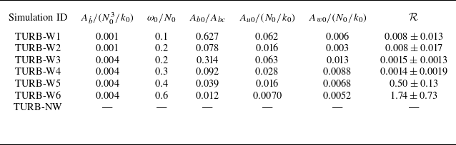
 Ab˙
 ω0
 Ab0/Abc
 Au0
 Aw0
 R
 R>1

 N0t=50
 N0t=200
 x
 u
 y=0
 b
 y=0
 y
 v
 x=0
 ϵ
 y=0
 u~=uk0/N0
 b~=bk0/N02

 z>0
 K~T
 Z~T
 z<0
 x
 y
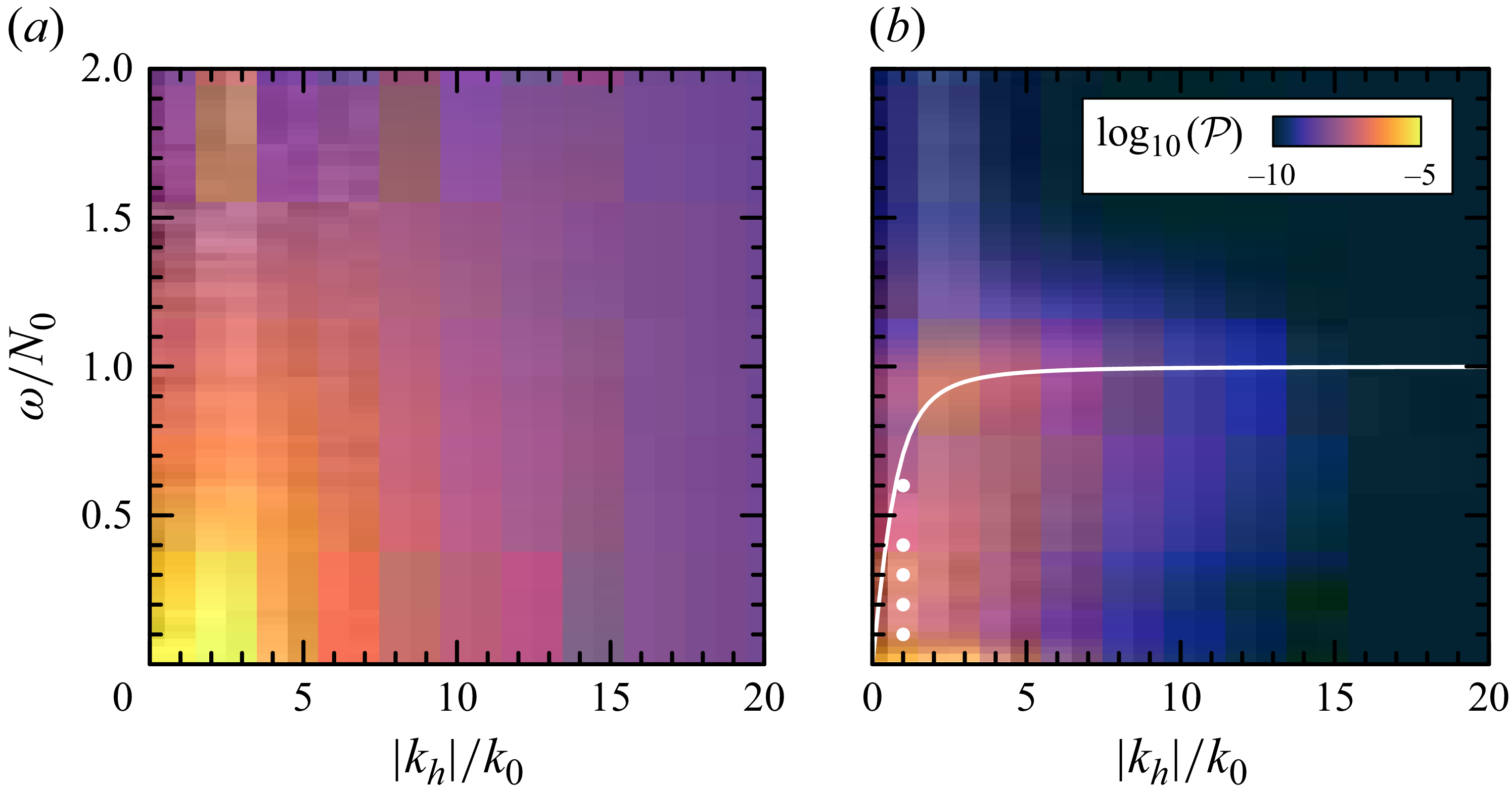
 P
 z=L/4
 z=−L/4
 kz=k0

 x
 u
 0.2N0
 kz<0
 kz>0
 0.2N0

 y=0
 u~=uk0/N0
 b~=bk0/N02
 t=200N0−1
 zw/L≃−0.26±0.04
 ω=0.2N0
 Ab˙=0.001N03/k0
 t∼(62±31)N0−1

 ω0=0.2N0
 Ab˙=0.001N03/k0

 x
 ⟨u⟩
 kx=k0
 c0=ω0/k0=0.2
 ⟨u⟩≪c0
 z=zw
 z=zw±σw
 z=0
 ±σt

 ω0=0.1N0
 Ab˙=0.001N03/k0
 ω0=0.2N0
 Ab˙=0.004N03/k0
 ω0=0.3N0
 Ab˙=0.004N03/k0
 ω0=0.4N0
 Ab˙=0.004N03/k0
 ω0=0.6N0
 Ab˙=0.004N03/k0
 u
 t=200N0
 kz<0
 ω0
 kz>0
 kx=k0
 ω0
 kz<0

 u
 t=150N0−1
 ω0=0.2N0
 Ab˙=0.004N03/k0

 NT2=N02+db¯/dz
 ω0=0.2N0
 Ab˙=0.001N03/k0
 u
 kz<0
 ω0
 ω0=0.6N0

 Open access

