2.1 Pipe flow

The pipe flow experiments are conducted at the Centre for International Cooperation in Long Pipe Experiments (CICLoPE) facility belonging to the University of Bologna, located in Predappio, Italy. The inner diameter of this unique large-scale facility is 0.9 m, with the measurement station located at the downstream end of a 111 m long pipe, where a fully developed turbulent pipe flow, for the first- and second-order statistics, is established (Örlü et al. Reference Örlü, Fiorini, Segalini, Bellani, Talamelli and Alfredsson2017). The large dimension for the outer length scale, $R$ , corresponding in this case to the pipe radius, allows access to high Reynolds numbers while the smallest energetic scales still remain $O(10~\unicode[STIX]{x03BC}\text{m})$ and therefore can be resolved using conventional techniques (Talamelli et al. Reference Talamelli, Persiani, Fransson, Alfredsson, Johansson, Nagib, Rüedi, Sreenivasan and Monkewitz2009). For further technical and flow characterisation details on the facility, the readers are referred to Bellani & Talamelli (Reference Bellani and Talamelli2016), Willert et al. (Reference Willert, Soria, Stanislas, Klinner, Amili, Eisfelder, Cuvier, Bellani, Fiorini and Talamelli2017) and Örlü et al. (Reference Örlü, Fiorini, Segalini, Bellani, Talamelli and Alfredsson2017). 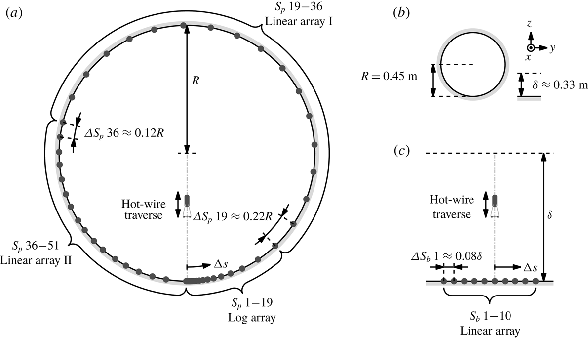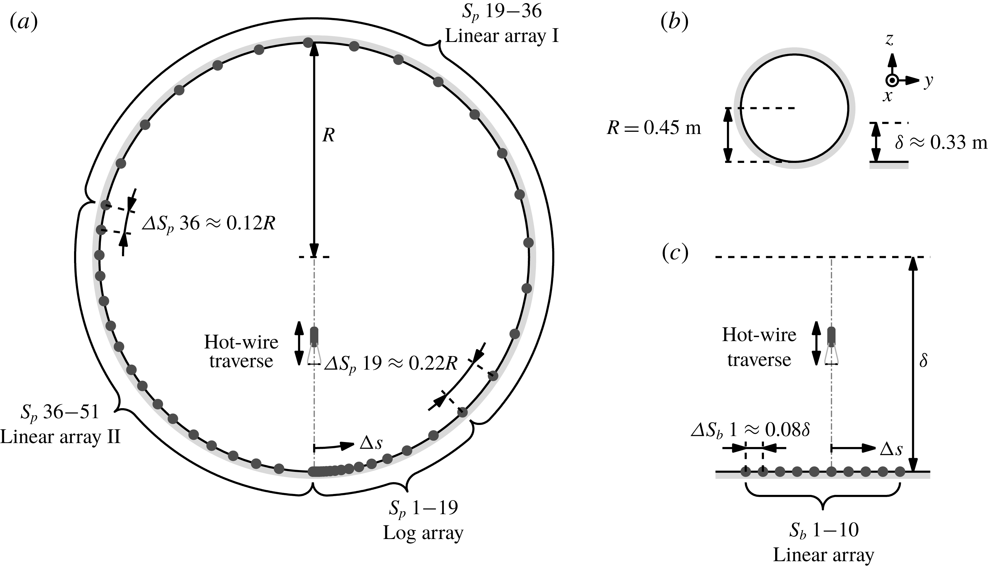The current experimental set-up consists of an array of 51 skin friction sensors located at various azimuthal positions spanning from 0– $2\unicode[STIX]{x03C0}$ along the pipe circumference simultaneously sampled with a hot-wire probe, nominally located at the same $x$ location as the hot-films. In addition, the hot-wire probe can be traversed from near the wall to the pipe centreline as shown in figure 1(a). It should be noted that the large pipe also allows the skin friction to be better resolved in the azimuthal direction by virtue of being able to accommodate a larger number of sensors along the circumference (see figure 1), compared to an alternate approach to high Reynolds numbers that relies on small $\unicode[STIX]{x1D708}/U_{\unicode[STIX]{x1D70F}}$ , typically achieved through reduction of the kinematic viscosity (e.g. Zagarola & Smits Reference Zagarola and Smits1998).

Table 1.

Summary of experimental conditions; $U_{CL}$ and $U_{\infty }$ denote the centreline and free-stream velocities in the pipe and boundary layer flows, while $T_{s}$ corresponds to the total sampling time at each wall-normal location, $z$ .

Figure 1.

Schematic of experimental set-ups. (a,c) Show locations of hot-film (●) and hot-wire sensors (not to scale) for the pipe and boundary layer flows, while (b) shows comparison of the outer length scales $R$ and $\unicode[STIX]{x1D6FF}$ respectively, in physical units.

Table 2.

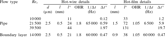
Summary of velocity and skin friction sensors utilised. OHR denotes the overheat ratio used for each sensor, while $1/\unicode[STIX]{x0394}t$ corresponds to the sampling frequency.

The velocity sensor is a hot-wire consisting of a Wollaston wire mounted onto a modified 55P15-type Dantec probe and etched to expose a $2.5~\unicode[STIX]{x03BC}\text{m}$ diameter platinum core of 0.5 mm length. The platinum wire is heated and maintained at a constant temperature with an overheat ratio of 1.8 using a Dantec StreamLine Pro anemometer system. Furthermore, here we maintain a hot-wire length ( $l$ ) to diameter ( $d$ ) ratio of 200 to avoid contamination from end conduction (Ligrani & Bradshaw Reference Ligrani and Bradshaw1987). Before and after each experiment, the hot-wire is traversed close to the centreline ( ${\sim}0.93R$ due to the limited range of the traverse) and the mean voltage is calibrated in situ against the centreline velocity, which is measured using a Pitot-static tube. This allows construction of a one-to-one relationship between the flow velocity and the anemometer output voltage. Although this means that calibration is not performed in a near-potential flow, the ratio $\sqrt{\,\overline{u^{2}}}/U$ at the centreline is sufficiently small to make insignificant differences to the potential flow calibration (Monty Reference Monty2005; Örlü et al. 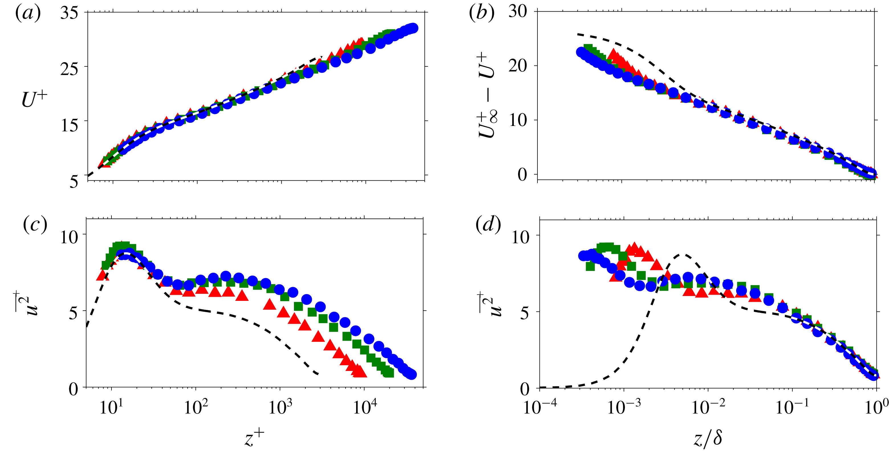Reference Örlü, Fiorini, Segalini, Bellani, Talamelli and Alfredsson2017). An intermediate calibration relationship between the hot-wire voltages and velocities is generated for each wall-normal point during the measurement, based on an assumption that deviations between pre- and post-calibration curves are the result of a linear drift in the hot-wire voltage with time. Figure 2(a,b) shows comparisons of the streamwise velocity mean profiles from the pipe experiments (denoted by symbols) against the dataset of Ahn et al. (Reference Ahn, Lee, Lee, Kang and Sung2015). Despite the departure from ideal calibration conditions, the $U$ profiles from the current datasets show good agreement with the DNS of Ahn et al. (Reference Ahn, Lee, Lee, Kang and Sung2015) (- - -) in the inner region when scaled in viscous units. In addition, a good agreement with the DNS is also observed for the deficit profiles in the outer region. Unlike the mean, the measured variance profiles are dependent on the sensor spatial resolution (Ligrani & Bradshaw Reference Ligrani and Bradshaw1987; Hutchins et al. Reference Hutchins, Nickels, Marusic and Chong2009). For the variance profiles shown in figure 2(c,d), the spatial resolution in the azimuthal direction varies from 6 viscous units between the adjacent grids (at the wall) for the DNS to 40 viscous units for the $Re_{\unicode[STIX]{x1D70F}}\approx 40\,000$ dataset from the current experiment. However, since the influence of the spatial resolution diminishes with an increasing $z$ , a good collapse of the $\overline{u^{2}}$ profiles is observed for the region $z/R>0.1$ in the outer scaling. Our $U$ and $\overline{u^{2}}$ results and the conclusions drawn agree with the findings of Örlü et al. (Reference Örlü, Fiorini, Segalini, Bellani, Talamelli and Alfredsson2017) from the same facility. Note, the present analysis is particularly insensitive to slight calibration differences (including the mismatch in the $z$ locations between the hot-wire probe and Pitot-static tube during calibration) since only relative changes in the skin friction and $u$ velocity are considered.

Figure 2.

Streamwise velocity statistics from the pipe experiments. Panels (a,b) and (c,d) show the mean and variance profiles, respectively. The symbols denote different $Re$ cases, i.e. ▴: $Re_{\unicode[STIX]{x1D70F}}\approx 10\,000$ ( $l^{+}=11$ ), ▪: $Re_{\unicode[STIX]{x1D70F}}\approx 22\,000$ ( $l^{+}=24$ ) and ●: $Re_{\unicode[STIX]{x1D70F}}\approx 40\,000$ ( $l^{+}=44$ ), while the dashed (- - -) lines correspond to the statistics from Ahn et al. (Reference Ahn, Lee, Lee, Kang and Sung2015) at $Re_{\unicode[STIX]{x1D70F}}\approx 3000$ ( $2\unicode[STIX]{x03C0}R^{+}/N_{\unicode[STIX]{x1D703}}=6$ , where $N_{\unicode[STIX]{x1D703}}$ is the number of grids in the DNS along the azimuthal direction).

Figure 3.

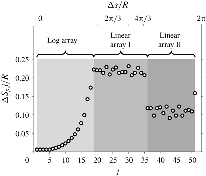
Azimuthal spacing, $\unicode[STIX]{x0394}S_{p}$ , between the adjacent sensors in the hot-film array for the pipe experiment.

Senflex hot-film sensor arrays from Tao systems are used to measure the skin friction. The three configurations depicted in figure 1(a) are used: a log array, a linear array I and a linear array II. The closely spaced sensors around the hot-wire traverse plane capture the small-scale contributions to the two-point statistics between $u$ and $u_{\unicode[STIX]{x1D70F}}$ , while the coarsely spaced sensors capture the large-scale contributions (these lose coherence much more gradually with increasing azimuthal offset, $\unicode[STIX]{x0394}s$ ). The azimuthal offsets of the sensors in the log array increase logarithmically from $\unicode[STIX]{x0394}s/R\approx 0.006$ to 0.22. Following the log array, the spacing in the linear array I is maintained at $\unicode[STIX]{x0394}s/R\approx 0.22$ from the 20th to 35th sensor. This spacing is halved to form linear array II. Furthermore, the sensors $S_{p}$ 1–17 are printed on to a single substrate, allowing the azimuthal offsets to be precisely set, while the remainder are manually positioned and the offsets recorded. The hot-wire is set to traverse nominally in the same plane as $S_{p}$ $2$ . Figure 3 shows the azimuthal offset between the adjacent hot-film sensors for the pipe experiment, where $\unicode[STIX]{x0394}S_{p}$ $j$ denotes the spacing between the $j$ and $j+1$ th sensors. To calibrate the hot-film sensors, the mean voltage outputs are recorded against the mean shear stress, obtained from measuring the axial pressure drop in the pipe before and after each experiment. The calibration curve for the hot-films follows a similar technique described for the hot-wire previously. However, since the hot-films are fixed in space, the voltage drift over time can be estimated throughout the measurement without the need for interpolation. Each of the 51 hot-films is operated by individual Melbourne University Constant Temperature Anemometer (MUCTA), Dantec StreamLine, AA labs AN1003 and Dantec Multichannel Constant Temperature Anemometers, each set to an overheat ratio of 1.05.

To ensure that the 51 hot-film voltages and the hot-wire voltage are acquired simultaneously, a common clock signal is utilised across five data translation DT9836 data acquisition boards used for analogue-to-digital conversion. To accommodate a faster temporal response expected from the hot-wire, it is sampled at a higher frequency than the hot-films. Furthermore, the two frequencies are chosen such that their ratio is an integer, thus allowing the hot-wire signal to be downsampled at the hot-film sampling frequency. In addition, a common hot-film voltage is shared between the five acquisition boards which is then used to verify the synchronicity of the acquisition. The hot-wire and hot-film details are summarised in table 2.

2.2 Boundary layer flow

The boundary layer dataset is from Hutchins et al. (Reference Hutchins, Monty, Ganapathisubramani, Ng and Marusic2011), which was acquired at the high Reynolds number boundary layer facility located at the University of Melbourne. The boundary layer thickness at the measurement location is approximately 0.33 m. As with the pipe experiments, this large $\unicode[STIX]{x1D6FF}$ allows access to the high $Re$ regime using conventional techniques (see figure 1 b for comparison against the pipe facility in physical units). Consistent with the pipe measurements, a $2.5~\unicode[STIX]{x03BC}\text{m}$ platinum Wollaston wire with a length to diameter ratio of 200 is used as a velocity sensor, while ten Dantec 55R47 glue-on-type hot-film sensors are used to measure the skin friction. The spanwise spacing between all ten hot-films is kept constant ( $\unicode[STIX]{x0394}S_{b}$ 1– $9\approx 0.08\unicode[STIX]{x1D6FF}$ ) and the hot-wire is located nominally above the sixth sensor, $S_{b}$ 6, as illustrated in figure 1(c). The hot-films and hot-wire are operated using AA labs AN1003 CTA systems with overheat ratios of 1.05 and 1.8, respectively. The hot-wire sensor is calibrated in the free stream against a Pitot-static tube before and after the measurement and linearly interpolated based on the working section temperature recorded during the measurement. The hot-film sensors are calibrated via an empirical relationship between the free-stream velocity and the mean wall-shear stress. For further details, the reader is referred to Hutchins et al. (Reference Hutchins, Monty, Ganapathisubramani, Ng and Marusic2011).

3.1 Single- and two-point statistics

Figure 4 shows the probability density function (p.d.f.) of friction velocity, ${\mathcal{P}}(u_{\unicode[STIX]{x1D70F}})$ , from the current dataset, where $u_{\unicode[STIX]{x1D70F}}=\sqrt{\unicode[STIX]{x1D70F}/\unicode[STIX]{x1D70C}}$ and $\unicode[STIX]{x1D70C}$ the density of the fluid. As is evident from the figure, the data merge across the range of Reynolds numbers examined, once $u_{\unicode[STIX]{x1D70F}}$ has been normalised by its standard deviation. Furthermore, this agreement extends to boundary layer flows where the friction velocity is measured using hot-films (♢). Also note that, in contrast to p.d.f. of wall-shear stress, ${\mathcal{P}}(\unicode[STIX]{x1D70F})$ , which is positively skewed (de Silva et al. Reference de Silva, Gnanamanickam, Atkinson, Buchmann, Hutchins, Soria and Marusic2014), ${\mathcal{P}}(u_{\unicode[STIX]{x1D70F}})$ is near symmetric. The missing contributions from small scales in the hot-film measurements are primarily associated with the unresolved skin friction contributions from the near-wall dynamics. In contrast, the well-resolved large-scale contributions are associated with larger structures residing in the logarithmic region. Since the $u$ velocity is less Gaussian in the near wall ( $z^{+}\lesssim 20$ ) than in the logarithmic region, this leads to a more Gaussian p.d.f. when compared to a better-resolved dataset (- - -) obtained using high-magnification particle image velocimetry (PIV) techniques (de Silva et al. Reference de Silva, Gnanamanickam, Atkinson, Buchmann, Hutchins, Soria and Marusic2014) (e.g. the skewness and kurtosis of $u_{\unicode[STIX]{x1D70F}}$ recorded by the hot-film are 0.15 and 2.9 respectively, in contrast to $-0.55$ and 7.2 obtained from the high-magnification PIV dataset).

Figure 4.

Probability density function of fluctuating friction velocity, ${\mathcal{P}}(u_{\unicode[STIX]{x1D70F}})$ . The solid symbols correspond to hot-film datasets from a pipe flow at $Re_{\unicode[STIX]{x1D70F}}\approx 10\,000$ (▴), 22 000 (▪) and 40 000 (●). Further, the open symbol (♢) and dashed line (- - -) show ${\mathcal{P}}(u_{\unicode[STIX]{x1D70F}})$ from a boundary layer flow at $Re_{\unicode[STIX]{x1D70F}}\approx 14\,000$ , obtained using hot-films and high-magnification PIV (de Silva et al. Reference de Silva, Gnanamanickam, Atkinson, Buchmann, Hutchins, Soria and Marusic2014), respectively. The solid line (——) indicates the standard normal distribution.

Figure 5.

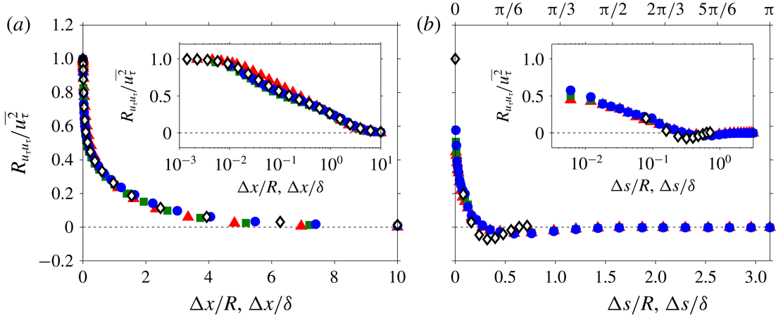
Two-point correlation of fluctuating friction velocity, $R_{u_{\unicode[STIX]{x1D70F}}u_{\unicode[STIX]{x1D70F}}}$ . The correlation coefficients are shown as functions of (a) the longitudinal ( $R_{u_{\unicode[STIX]{x1D70F}}u_{\unicode[STIX]{x1D70F}}}(\unicode[STIX]{x0394}x,0)$ ) and (b) transverse ( $R_{u_{\unicode[STIX]{x1D70F}}u_{\unicode[STIX]{x1D70F}}}(0,\unicode[STIX]{x0394}s)$ ) offsets. The solid symbols correspond to pipe flow at $Re_{\unicode[STIX]{x1D70F}}\approx 10\,000$ (▴), 22 000 (▪) and 40 000 (●), while the open symbols (♢) correspond to boundary layer flow at $Re_{\unicode[STIX]{x1D70F}}\approx 14\,000$ . For the insets, a logarithmic scale is used for the displacements, $\unicode[STIX]{x0394}x$ and $\unicode[STIX]{x0394}s$ , between the two points.

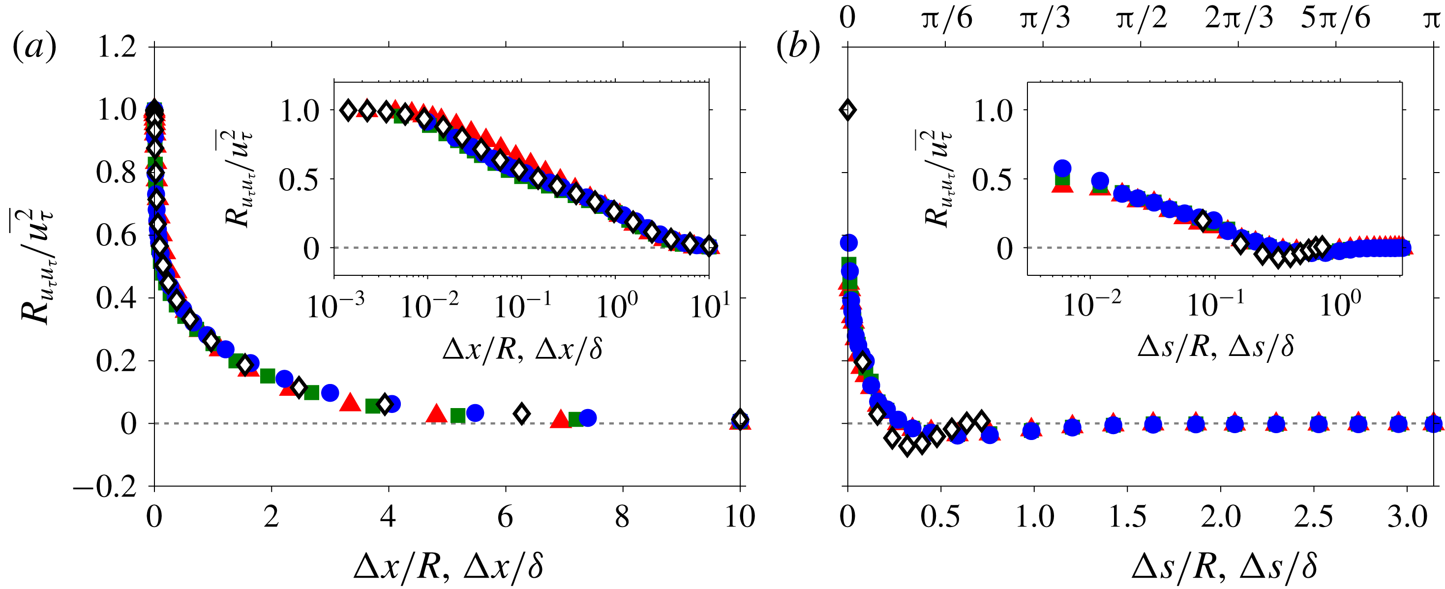
Figure 5(a,b) shows the two-point correlation of $u_{\unicode[STIX]{x1D70F}}$ , $R_{u_{\unicode[STIX]{x1D70F}}u_{\unicode[STIX]{x1D70F}}}$ from the current dataset as functions of longitudinal (streamwise) and transverse offsets, respectively. It should be noted that the streamwise offset, $\unicode[STIX]{x0394}x$ in (a) is obtained through use of Taylor’s frozen turbulence hypothesis (Taylor Reference Taylor1938), where a convection velocity, $U_{c}$ , is used to convert the hot-film signal from the temporal to the spatial domain. Following work of Hutchins et al. (Reference Hutchins, Monty, Ganapathisubramani, Ng and Marusic2011), who examined space–time correlation of two hot-film sensors separated in $x$ , the convection velocity for the large-scale $u_{\unicode[STIX]{x1D70F}}$ fluctuations is estimated to be the mean velocity at the $z$ location where the very-large-scale $u$ fluctuations are strongest (i.e. the large-scale $u_{\unicode[STIX]{x1D70F}}$ features convect at the same rate as the very-large-scale $u$ fluctuations residing in the logarithmic region). This wall height approximately corresponds to $z^{+}=\sqrt{15Re_{\unicode[STIX]{x1D70F}}}$ according to Mathis, Hutchins & Marusic (Reference Mathis, Hutchins and Marusic2009), hence based on the logarithmic law we obtain

(3.1) $$\begin{eqnarray}\displaystyle \frac{U_{c}}{U_{\unicode[STIX]{x1D70F}}}=\frac{1}{\unicode[STIX]{x1D705}}\ln \sqrt{15Re_{\unicode[STIX]{x1D70F}}}+A, & & \displaystyle\end{eqnarray}$$

where $\unicode[STIX]{x1D705}=0.39$ and $A=4.3$ are the Kármán constant and the logarithmic intercept for canonical wall-bounded flows (Marusic et al. Reference Marusic, Monty, Hultmark and Smits2013). Although the frozen turbulence hypothesis is known to breakdown for the small scales in the near-wall region (Piomelli, Balint & Wallace Reference Piomelli, Balint and Wallace1989; del Álamo & Jiménez Reference del Álamo and Jiménez2009), since the hot-film sensors only resolve large-scale contributions, it is a reasonable approximation for the signals obtained from these sensors. For the transverse offset, the correlation is calculated from two sensors separated by distance $\unicode[STIX]{x0394}s$ in the azimuthal and spanwise directions for the pipe and boundary layer flows, respectively. It should be also noted that, while only selective $\unicode[STIX]{x0394}x$ locations (corresponding to a specific $\unicode[STIX]{x0394}t$ offset in the $u_{\unicode[STIX]{x1D70F}}$ time series) are shown in figure 5(a), $\unicode[STIX]{x0394}s$ locations from each hot-film pair are shown in figure 5(b).

As is evident from figure 5(a,b), good agreement is observed for $R_{u_{\unicode[STIX]{x1D70F}}u_{\unicode[STIX]{x1D70F}}}$ from the current dataset (▴, ▪ and ●) for both streamwise and azimuthal offsets, when normalised by the outer length scale. This is because the correlations beyond $\unicode[STIX]{x0394}x/R,\unicode[STIX]{x0394}s/R>O(0.1)$ are dominated by the large-scale motions which scale with the outer length scale. Similar results have been observed for two-point correlations of streamwise velocity (Hutchins & Marusic Reference Hutchins and Marusic2007a ). However, for small $\unicode[STIX]{x0394}x$ , the collapse of $R_{u_{\unicode[STIX]{x1D70F}}u_{\unicode[STIX]{x1D70F}}}$ across different $Re$ is no longer expected when normalised by the outer length scale, since the scale separation between the viscous and inertially dominated scales increases with increasing $Re$ . This is also evident in the experimental data when a logarithmic scale is used for $\unicode[STIX]{x0394}x$ (e.g. figure 5 b inset), where $R_{u_{\unicode[STIX]{x1D70F}}u_{\unicode[STIX]{x1D70F}}}$ at $\unicode[STIX]{x0394}x/R\sim 0.1$ no longer exhibits a collapse. Notably, the collapse of $R_{u_{\unicode[STIX]{x1D70F}}u_{\unicode[STIX]{x1D70F}}}$ for a large $\unicode[STIX]{x0394}x$ extends to the boundary layer case (♢) when the streamwise offset distance is normalised by its respective outer length scale, as seen in figure 5(a). However, figure 5(b) shows that, unlike the streamwise offset, $R_{u_{\unicode[STIX]{x1D70F}}u_{\unicode[STIX]{x1D70F}}}$ from the pipe and boundary layer flows exhibit discernible differences in the transverse direction even after the offset has been normalised by the outer length scale. A similar difference between internal (channel and pipe) and external (boundary layer) flows is reported by Monty et al. (Reference Monty, Stewart, Williams and Chong2007) for correlations of $u$ . They attribute the differences to variations in the coherent structures that extend beyond the logarithmic region ( $z/R,z/\unicode[STIX]{x1D6FF}>0.15$ ). In internal flow, these coherent structures are persistent, while in the external flow they breakdown more readily into smaller eddies, resulting in $R_{u_{\unicode[STIX]{x1D70F}}u_{\unicode[STIX]{x1D70F}}}$ decreasing faster in the transverse direction. As a result, the anti-correlated region where $R_{u_{\unicode[STIX]{x1D70F}}u_{\unicode[STIX]{x1D70F}}}$ is most negative shifts from $\unicode[STIX]{x0394}s/R\approx 0.6$ to $\unicode[STIX]{x0394}s/\unicode[STIX]{x1D6FF}\approx 0.4$ between the internal and external flows (see figure 5 b), replicating the $R_{uu}$ behaviour observed in the logarithmic region (Sillero, Jiménez & Moser Reference Sillero, Jiménez and Moser2014).

3.2 Instantaneous visualisations

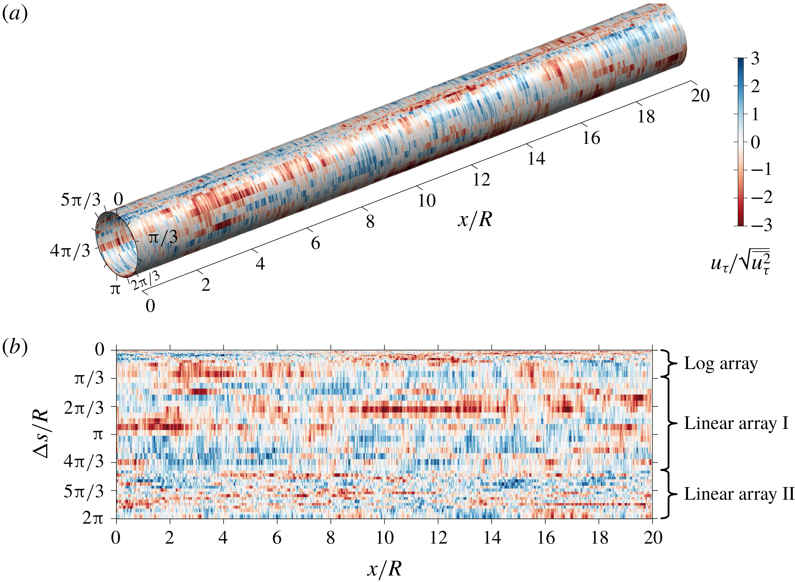
Figure 6 shows an instantaneous view of the friction velocity from the current dataset, at $Re_{\unicode[STIX]{x1D70F}}\approx 40\,000$ . Since the spacing between the hot-films is $0.1R$ – $0.2R$ for the two linear arrays (covering almost 85 % of the total pipe circumference), the $R$ -scaled features dominate the instantaneous view. These $R$ -scaled features are associated with very-large-scale motions (VLSMs) (Kim & Adrian Reference Kim and Adrian1999) that largely reside in the logarithmic region and whose influence extends down to the wall (Hutchins & Marusic Reference Hutchins and Marusic2007a ). Thus, these footprints impose large-scale $u_{\unicode[STIX]{x1D70F}}$ features that meander and extend over $O(10R)$ in the streamwise direction with a width of $O(R)$ in the azimuthal direction (Monty et al. Reference Monty, Stewart, Williams and Chong2007).

4.1 Comparisons between pipe and boundary layer flows

Figure 7.

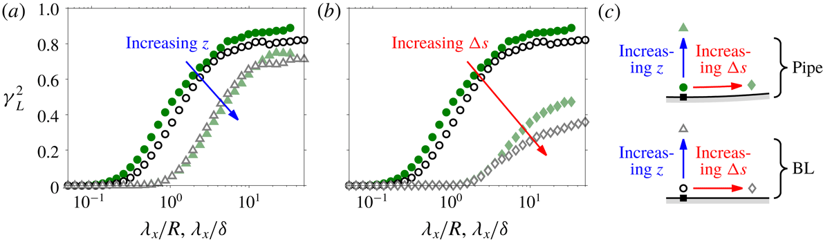
Coherence spectrum, $\unicode[STIX]{x1D6FE}_{L}^{2}$ , between the streamwise velocity, $u$ , and the friction velocity, $u_{\unicode[STIX]{x1D70F}}$ , as a function of wavelength $\unicode[STIX]{x1D706}_{x}$ . The solid (●, ▴, ♦) and open (○, ▵, ♢) symbols respectively correspond to the pipe and boundary layer (BL) flows. Also, the pipe and boundary layer flows are at $Re_{\unicode[STIX]{x1D70F}}\approx 22\,000$ and 14 000, respectively. (a) Two wall heights $z/R,z/\unicode[STIX]{x1D6FF}\approx 0.01$ (●, ○) and 0.07 (▴, ▵) at $\unicode[STIX]{x0394}s\approx 0$ ; and (b) two hot-film offsets $\unicode[STIX]{x0394}s/R,\unicode[STIX]{x0394}s/\unicode[STIX]{x1D6FF}\approx 0$ (●, ○) and 0.07 (♦, ♢) at $z/R,z/\unicode[STIX]{x1D6FF}\approx 0.01$ are shown. (c) Schematic of hot-wire and hot-film positions used to generate (a) and (b), where ▪ symbol denotes the reference skin friction sensor.

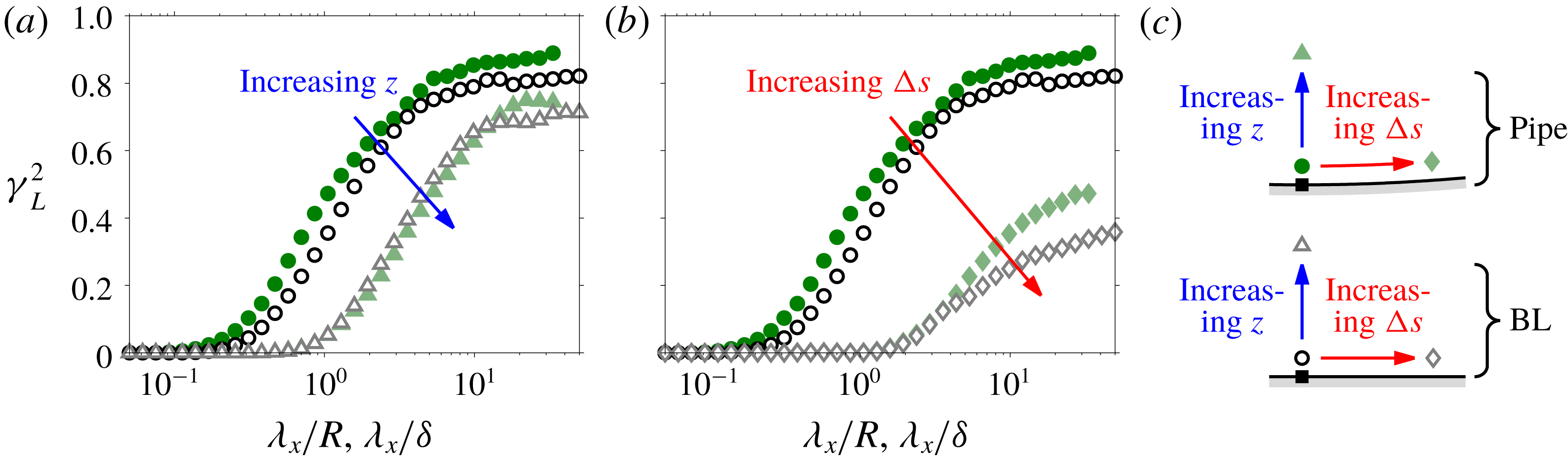
Figure 7(a,b) shows $\unicode[STIX]{x1D6FE}_{L}^{2}$ between the streamwise velocity, $u$ , and the friction velocity, $u_{\unicode[STIX]{x1D70F}}$ , as a function of wavelength $\unicode[STIX]{x1D706}_{x}$ . The solid circles (●) in both (a) and (b), correspond to the coherence spectrum for the pipe flow when $u$ is acquired at $z/R\approx 0.01$ and is measured directly above $u_{\unicode[STIX]{x1D70F}}$ , as illustrated in (c). Similarly, the empty circles (○) correspond to the coherence spectrum for the boundary layer flow, where $u$ is measured $0.01\unicode[STIX]{x1D6FF}$ above $u_{\unicode[STIX]{x1D70F}}$ .

Figure 8.

(a) Schematic showing a hierarchy of attached eddies used to model wall-bounded flows. Here, four hierarchy levels are shown, where a volume of influence from each is represented by a differently coloured cuboid, while the symbols indicate probe locations. (b) The contribution to $u$ or $u_{\unicode[STIX]{x1D70F}}$ signals at four locations (as indicated by corresponding symbols in a) over a streamwise distance $a$ ; ${\mathcal{L}}_{\,i},{\mathcal{W}}_{i}$ and ${\mathcal{H}}_{i}$ denote the streamwise, spanwise and wall-normal extents of an $i$ th hierarchy level eddy.

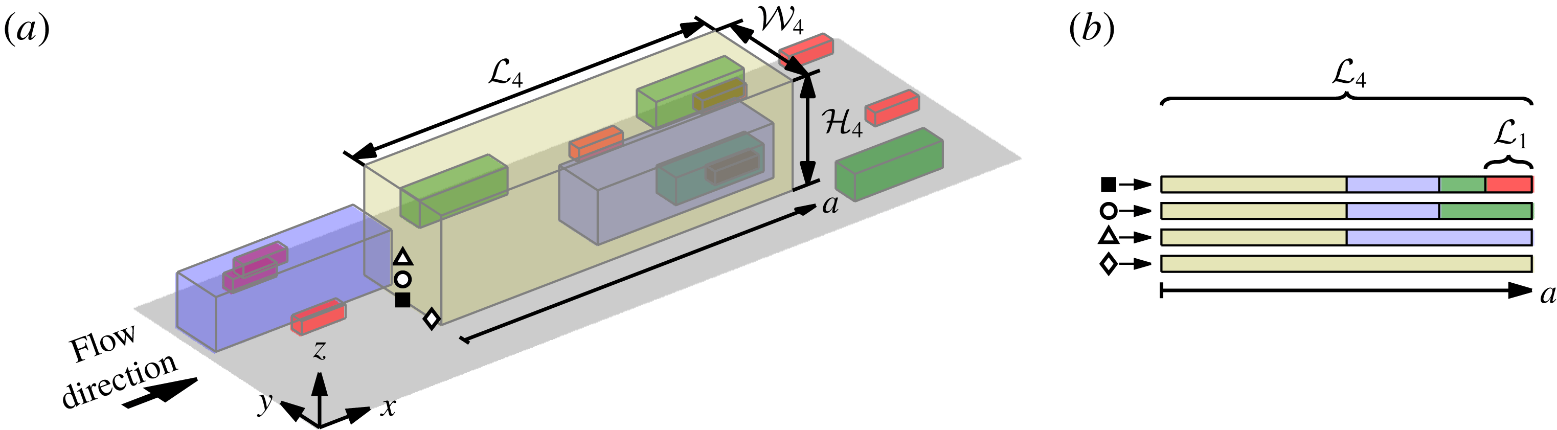
As stated in the introduction, one of the aims of this paper is to extend the observation of Baars et al. (Reference Baars, Hutchins and Marusic2017), which supports wall-bounded turbulence obeying the AEH. Figure 8 shows a sketch illustrating relative scales in the AEH, where a hierarchy of self-similar structures is used to represent the logarithmic region in a wall-bounded flow. The size of each hierarchy level is shown in a different colour, and the hierarchy follows a geometric progression with a common ratio of 2 up to a height equal to the outer length scale. In this schematic the population density halves in the $x$ and $y$ dimensions for each increment in the hierarchy level. Thus, in figure 8 a total of four hierarchy levels are shown, and eddies at each level have an extent in the $x$ , $y$ and $z$ directions characterised here by ${\mathcal{L}}_{\,i},{\mathcal{W}}_{i}$ and ${\mathcal{H}}_{i}$ , respectively. Here, subscript $i=1$ –4 is used to denote each hierarchy level, with the smallest and largest following ${\mathcal{H}}_{1}\sim O(\unicode[STIX]{x1D708}/U_{\unicode[STIX]{x1D70F}})$ and ${\mathcal{H}}_{4}\sim O(\unicode[STIX]{x1D6FF})$ , respectively (Perry & Chong Reference Perry and Chong1982). It should be noted that in reality, these structures are forward inclined relative to the flow direction (Robinson Reference Robinson1991). Since, however, only the magnitude of the coherence (and not the phase) is considered here, this detail is not relevant to the present discussion. Now, consider probes placed at ▪ (measuring $u_{\unicode[STIX]{x1D70F}}$ ) and ○ (measuring $u$ ) as illustrated in figure 8(a), leading to recorded signals from these probes as in figure 8(b). It is therefore evident that the signal from the ○ sensor misses contributions from the smallest eddies when compared to the signal from the ▪ sensor. In contrast, the large-scale component of these signals is still mostly coherent, leading to a steady decay in $\unicode[STIX]{x1D6FE}_{L}^{2}$ from ${\sim}0.8$ to 0 with decreasing $\unicode[STIX]{x1D706}_{x}$ , as observed in figure 7(a,b).

Figure 7(a) shows the effect of increased separation between $u$ and $u_{\unicode[STIX]{x1D70F}}$ in the $z$ direction. Here, ▵ symbols correspond to a case where $u$ is obtained at a higher $z$ location than the ○ symbols as illustrated in figure 7(c). A decrease in $\unicode[STIX]{x1D6FE}_{L}^{2}$ is observed at all scales in both the pipe and boundary layer flows with increased $z$ separation. In terms of the AEH, this relates to a reduction in the number of common members of the hierarchy encountered with increased $z$ , as shown by idealised $u$ signals at ○ and ▵ in figure 8(b). Similarly, figure 7(b) shows the effect of increased separation between $u$ and $u_{\unicode[STIX]{x1D70F}}$ in the transverse direction, with the ♢ symbol corresponding to a case where $u$ is obtained with an azimuthal/spanwise offset, $\unicode[STIX]{x0394}s$ , compared to the ○ symbols as indicated in figure 7(c). Again, a decrease in $\unicode[STIX]{x1D6FE}_{L}^{2}$ at all scales is observed in both the pipe and boundary layer flows with increased $\unicode[STIX]{x0394}s$ separation, but the decrease is much more severe compared to that observed for an equivalent increase in $z$ . As discussed later, these differences can also be explained by considering an idealised model based on the AEH.

Figure 9.

Coherence spectrum between $u_{\unicode[STIX]{x1D70F}}$ and $u$ , $\unicode[STIX]{x1D6FE}_{L}^{2}$ , as a function of wavelength, $\unicode[STIX]{x1D706}_{x}$ , and wall-normal location, $z$ , where $u$ is measured. (a,c) Pipe $Re_{\unicode[STIX]{x1D70F}}\approx 22\,000$ and (b,d) boundary layer $Re_{\unicode[STIX]{x1D70F}}\approx 14\,000$ flows, where $z$ is shown in linear and logarithmic scale on the top (a,b) and bottom (c,d) rows, respectively. The grey scale contours correspond to coherence when the hot-film sensor (▪) is at an offset of $\unicode[STIX]{x0394}s\approx 0$ from the hot-wire (●), while the line contours show coherence at an offset of $\unicode[STIX]{x0394}s/R,\unicode[STIX]{x0394}s/\unicode[STIX]{x1D6FF}\approx 0.07$ (▫). Both line and grey scale contours are at levels 0.1:0.1:0.9, and the dash-dotted lines indicate the $\unicode[STIX]{x1D706}_{x}=A_{xz}\,z$ relationship, where $A_{xz}=14$ corresponds to empirically observed aspect ratio between $\unicode[STIX]{x1D706}_{x}$ and $z$ for the self-similar hierarchy.

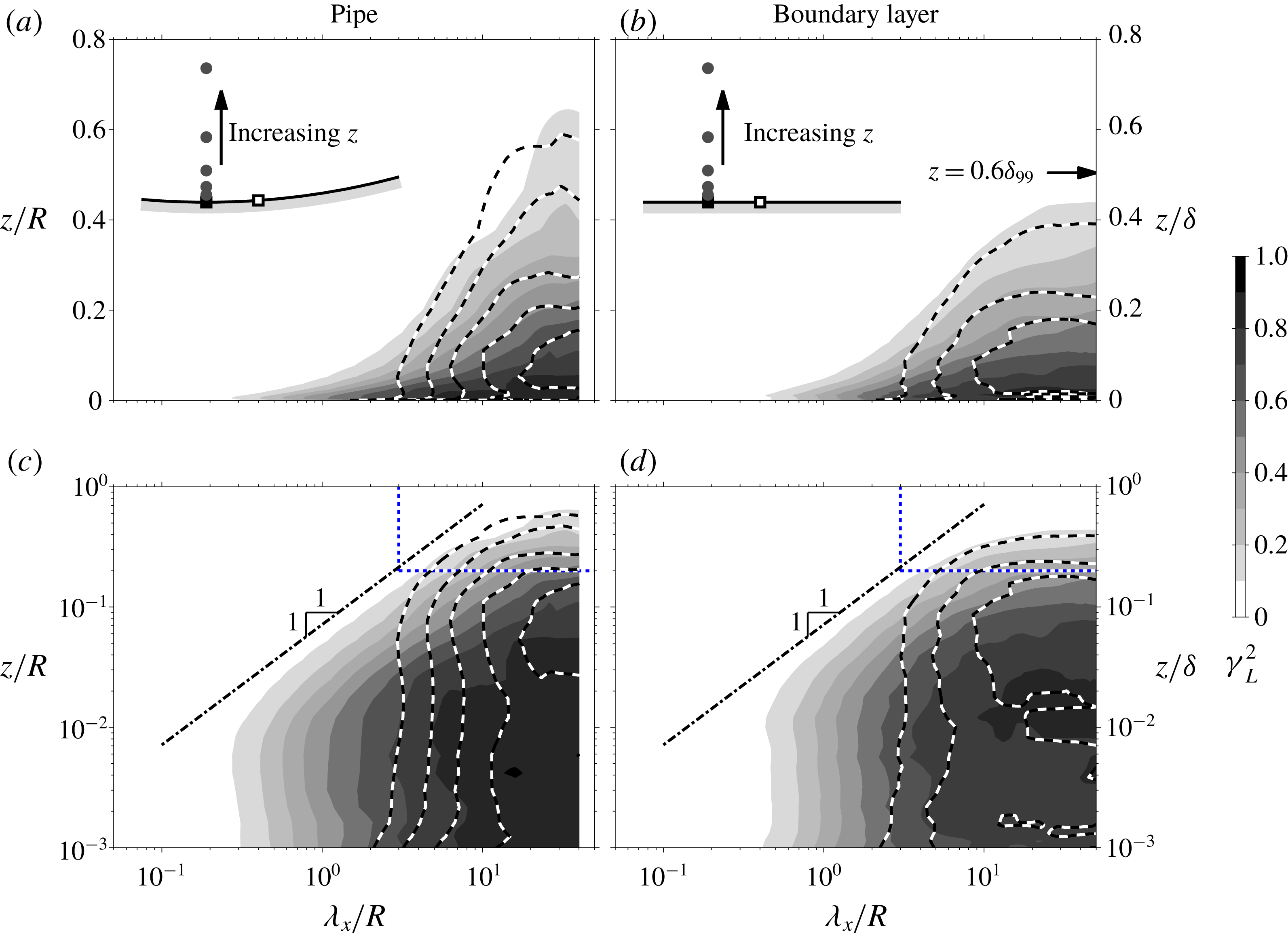
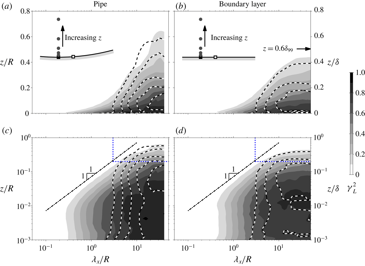
Figure 9 shows coherence spectra as functions of $\unicode[STIX]{x1D706}_{x}$ and $z$ . The left (a,c) and right (b,d) figures correspond to $\unicode[STIX]{x1D6FE}_{L}^{2}$ for the pipe and boundary layer flows, respectively. The top (a,b) and bottom (c,d) figures correspond to the same coherence spectra, but $z$ is shown in the linear and logarithmic scales, respectively. It should be noted that there exists a slight discrepancy in $Re_{\unicode[STIX]{x1D70F}}$ between the two flows (22 000 for the pipe compared to 14 000 for the boundary layer), however across this range, we expect the $Re_{\unicode[STIX]{x1D70F}}$ effects on the large-scale features to be minimal when scaled by the outer length scales (Hutchins & Marusic Reference Hutchins and Marusic2007a ,Reference Hutchins and Marusic b ). Consequently, here we present $\unicode[STIX]{x1D706}_{x}$ and $z$ normalised by $R$ and $\unicode[STIX]{x1D6FF}$ respectively for the pipe and boundary layer flows.

From figure 9(a,b), it is evident that the large-scale component of $u$ motions remains coherent over a larger $z$ extent for the pipe compared to the boundary layer flow when normalised by the corresponding outer length scale, in agreement with the observations of Monty et al. (Reference Monty, Stewart, Williams and Chong2007). In an internal flow such as a pipe, instances exist where a large-scale $u$ event remains coherent over a $z$ extent larger than $R$ (i.e. penetrates beyond the centreline while starting at the wall) (Sillero et al. Reference Sillero, Jiménez and Moser2014), while $\unicode[STIX]{x1D6FF}$ for the boundary layer flow is closer to the outermost edge of the turbulent region, and beyond which only a non-turbulent flow exists (Chauhan et al. Reference Chauhan, Philip, de Silva, Hutchins and Marusic2014). This mismatch in the outer length scale used for the normalisation relative to the size of the largest coherent motions presumably leads to some of the differences observed between the coherence spectra from the pipe and boundary layer flow in the wake region. It should be noted that, a choice of $\unicode[STIX]{x1D6FF}_{99}$ (i.e. the $z$ location where $U=0.99U_{\infty }$ ) as the outer length scale for the boundary layer instead of $\unicode[STIX]{x1D6FF}$ , yields a better agreement in the wake region as evident from the $z=0.6\,\unicode[STIX]{x1D6FF}_{99}$ position indicated on figure 9(b). Despite the modification to the choice of outer length scale, the differences in the $u$ -spectra between the internal and external flows still persist, since as demonstrated by Monty et al. (Reference Monty, Hutchins, Ng, Marusic and Chong2009), it is not possible to achieve a full merging of the $u$ -spectra across the entire large wavelength range, irrespective of the outer length-scale definition chosen.

Another potential source of difference between the internal and external flows in figure 9(a,b), may be due to use of Reynolds decomposition in obtaining the $u$ fluctuations. While this is a standard practice, if multiple states with different mean exist in a flow (such as turbulent and non-turbulent regions), all states are reduced to a single common mean (Kwon, Hutchins & Monty Reference Kwon, Hutchins and Monty2016). Hence, the use of Reynolds decomposition can exacerbate observed differences between internal and external flows under outer scaling, as demonstrated by Kwon (Reference Kwon2016), who improved the collapse of the two-point correlation of a boundary layer and a channel using an alternate decomposition that separated the turbulent and quiescent core/non-turbulent regions. However, it should also be noted that both choices for the $u$ fluctuations provide similar results in the logarithmic and near-wall regions as the turbulent portion dominates at these $z$ locations.

The grey scale contours in figure 9 correspond to the coherence spectra between $u_{\unicode[STIX]{x1D70F}}$ and $u$ for $\unicode[STIX]{x0394}s\approx 0$ , while the line contours show $\unicode[STIX]{x1D6FE}_{L}^{2}$ when an azimuthal/spanwise offset of $\unicode[STIX]{x0394}s/R,\unicode[STIX]{x0394}s/\unicode[STIX]{x1D6FF}\approx 0.07$ exists between the hot-film and hot-wire (see inset, symbols ▫ and ●). Based on the attached eddy model illustrated in figure 8, we would expect the two hot-film sensors to share large-scale $u_{\unicode[STIX]{x1D70F}}$ features since they share a common footprint from eddies that span across both sensors. This is indeed reflected in figure 9, where the two coherence spectra at $\unicode[STIX]{x0394}s=0$ and $\unicode[STIX]{x0394}s/R,\unicode[STIX]{x0394}s/\unicode[STIX]{x1D6FF}\approx 0.07$ show good agreement for $\unicode[STIX]{x1D706}_{x}/R,\unicode[STIX]{x1D706}_{x}/\unicode[STIX]{x1D6FF}>3$ and $z/R,z/\unicode[STIX]{x1D6FF}>0.2$ (top-right regions encapsulated by the dotted lines in figure 9 c,d). As the effect of the differing outer boundary conditions between the internal and external flow is diminished closer to the wall, a good agreement is also observed between the pipe and boundary layer flows (see figure 9 c,d) in the logarithmic region. This includes the iso-contours of the coherence spectra following a $\unicode[STIX]{x1D706}_{x}\sim z$ scaling (shown as dot-dashed lines). This behaviour is consistent with the AEH, which assumes that the coherent structures are self-similar and scale with the distance from the wall (Townsend Reference Townsend1976). The dash-dotted lines in figure 9(c,d) shows the relationship $\unicode[STIX]{x1D706}_{x}=A_{xz}\,z$ , where $A_{xz}=14$ corresponds to $\unicode[STIX]{x1D706}_{x}$ where wall-shear stress and $u$ velocity starts to exhibit coherence in the logarithmic region (Baars et al. Reference Baars, Hutchins and Marusic2017). Thus, these features are much longer in $x$ compared to their $z$ -extent (i.e. $A_{xz}\gg 1$ ), indicating that the coherent motions in $u$ are likely associated with multiple streamwise aligned eddies travelling in a packet (Adrian, Meinhart & Tomkins Reference Adrian, Meinhart and Tomkins2000), rather than a single isolated eddy.

Figure 10.

An illustration of size of an $i$ th hierarchy level eddy, ${\mathcal{L}}_{\,i}\times {\mathcal{W}}_{i}\times {\mathcal{H}}_{i}$ , extracted based on $\unicode[STIX]{x1D706}_{x}$ , $\unicode[STIX]{x0394}s$ and $z$ where $\unicode[STIX]{x1D6FE}_{L}^{2}=\unicode[STIX]{x1D6E4}$ ( $\unicode[STIX]{x1D6E4}$ is a threshold). (a) Wall-parallel ( $x$ – $y$ plane) view of volume of influence and (b) cross-plane ( $y$ – $z$ plane) view (along A–A in a) showing different scenarios where the volume of influence passes over a reference skin friction sensor (▪). The blue and red regions in (a,b) denote negative and positive $u$ , respectively, while $x^{\prime }$ , $y^{\prime }$ and $z^{\prime }$ are coordinates relative to the eddy. The solid lines in (c,d) show idealised coherence as a function of offset distances $z$ and $\unicode[STIX]{x0394}s$ between the two sensors in the wall-normal and spanwise directions, respectively. The dashed line in (d) shows an equivalent step-like profile proposed.

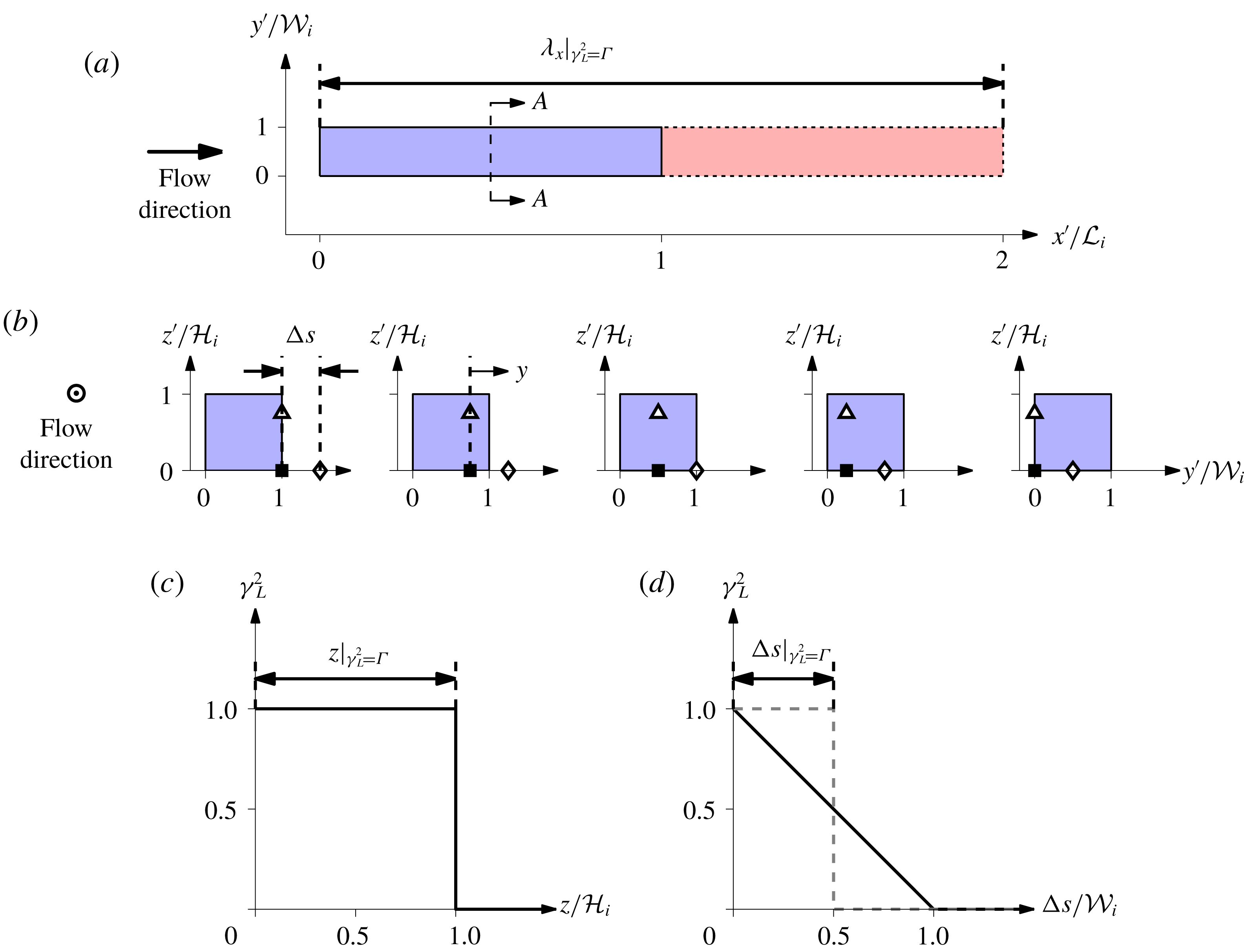
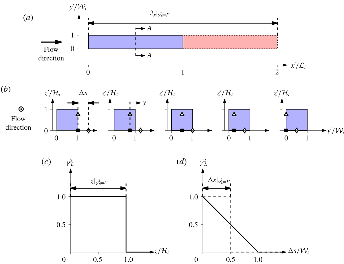
Here, we propose to characterise the dimensions ( ${\mathcal{L}}\times {\mathcal{W}}\times {\mathcal{H}}$ ) of the self-similar attached eddies based on $\unicode[STIX]{x1D6FE}_{L}^{2}$ iso-contours, following Baars et al. (Reference Baars, Hutchins and Marusic2017). Note that, while the attached eddies are confined in the wall-normal direction by the presence of the wall, no such confinement exists in the spanwise direction leading to differences in how $\unicode[STIX]{x1D6FE}_{L}^{2}$ approaches zero as a function of $\unicode[STIX]{x0394}s$ and $z$ (e.g. figure 7). As an example, consider the idealised, discrete eddy, scenario shown in figure 8, when an eddy passes over a reference skin friction sensor. As illustrated in figure 10(b), this requires the reference skin friction sensor (denoted by symbol ▪) to be located within the low shear stress footprint of the eddy with an equal probability. For a case when the shear stress and velocity sensors are spanwise aligned, the velocity recorded at a wall-normal offset $z$ , $u(z)$ , is perfectly correlated with the wall-shear stress sensor ( $\unicode[STIX]{x1D6FE}_{L}^{2}=1$ ) if $z<{\mathcal{H}}_{i}$ , otherwise the two signals remain uncorrelated ( $\unicode[STIX]{x1D6FE}_{L}^{2}=0$ ), regardless of the spanwise position of the eddy, leading to a step like $\unicode[STIX]{x1D6FE}_{L}^{2}$ as a function of $z$ as shown in figure 10(c). In contrast, for a case when $\unicode[STIX]{x0394}s\neq 0$ , the likelihood that influence of the eddy extends to $y=\unicode[STIX]{x0394}s$ is no longer equal to unity even when $z<{\mathcal{H}}_{i}$ . This is because unlike the $\unicode[STIX]{x0394}s=0$ case, there are instances when the eddy does not span across the two sensors as illustrated in figure 10(b). Furthermore from the figure, it is evident that the portion of eddies that reach $y=\unicode[STIX]{x0394}s$ decreases linearly with increasing $\unicode[STIX]{x0394}s$ until $\unicode[STIX]{x0394}s={\mathcal{W}}_{i}$ , from which point onwards the signals from the two sensors remain uncorrelated. Therefore, $\unicode[STIX]{x1D6FE}_{L}^{2}=\max (1-\unicode[STIX]{x0394}s/{\mathcal{W}}_{i},0)$ for this idealised case, as illustrated in figure 10(d). In order to resolve the difference in $\unicode[STIX]{x1D6FE}_{L}^{2}$ as a function of $\unicode[STIX]{x0394}s$ and $z$ , here we propose that the linear $\unicode[STIX]{x1D6FE}_{L}^{2}$ dependency with $\unicode[STIX]{x0394}s$ can be transformed to an equivalent step-like function observed for $z$ by preserving the area under the graph, in a similar manner to how an integral scale is inferred from $R_{uu}$ . It should also be noted that the procedure is related to a ‘coherence height’ as defined by Jiménez, del Álamo & Flores (Reference Jiménez, del Álamo and Flores2004). In the present case, however, the integration is carried out in the spanwise direction. Based on these arguments, we propose to extract ${\mathcal{H}}_{i}$ and ${\mathcal{W}}_{i}$ based on $z$ and $\unicode[STIX]{x0394}s$ locations where $\unicode[STIX]{x1D6FE}_{L}^{2}=\unicode[STIX]{x1D6E4}$ (here $\unicode[STIX]{x1D6E4}$ corresponds to a threshold), leading to ${\mathcal{H}}_{i}=z|_{\unicode[STIX]{x1D6FE}_{L}^{2}=\unicode[STIX]{x1D6E4}}$ and ${\mathcal{W}}_{i}=2\unicode[STIX]{x0394}s|_{\unicode[STIX]{x1D6FE}_{L}^{2}=\unicode[STIX]{x1D6E4}}$ , respectively. For the streamwise extent since the coherence spectra are employed, ${\mathcal{L}}_{\,i}=0.5\unicode[STIX]{x1D706}_{x}|_{\unicode[STIX]{x1D6FE}_{L}^{2}=\unicode[STIX]{x1D6E4}}$ , as negative $u$ fluctuations only remain coherent over half of the total wavelength, and because of association with the Fourier transform a positive $u$ fluctuation portion of the same size follows to form one full wavelength as indicated in figure 10(a) (blue and red regions denote negative and positive $u$ , respectively). In the later section, we obtain the mean dimensions, ${\mathcal{L}}_{\,i}\times {\mathcal{W}}_{i}\times {\mathcal{H}}_{i}$ , of the attached eddies that lead to a self-similar hierarchy in the logarithmic region, and show that they agree with previous studies that have examined the in-plane dimensions at a similar $Re$ .

Figure 11.

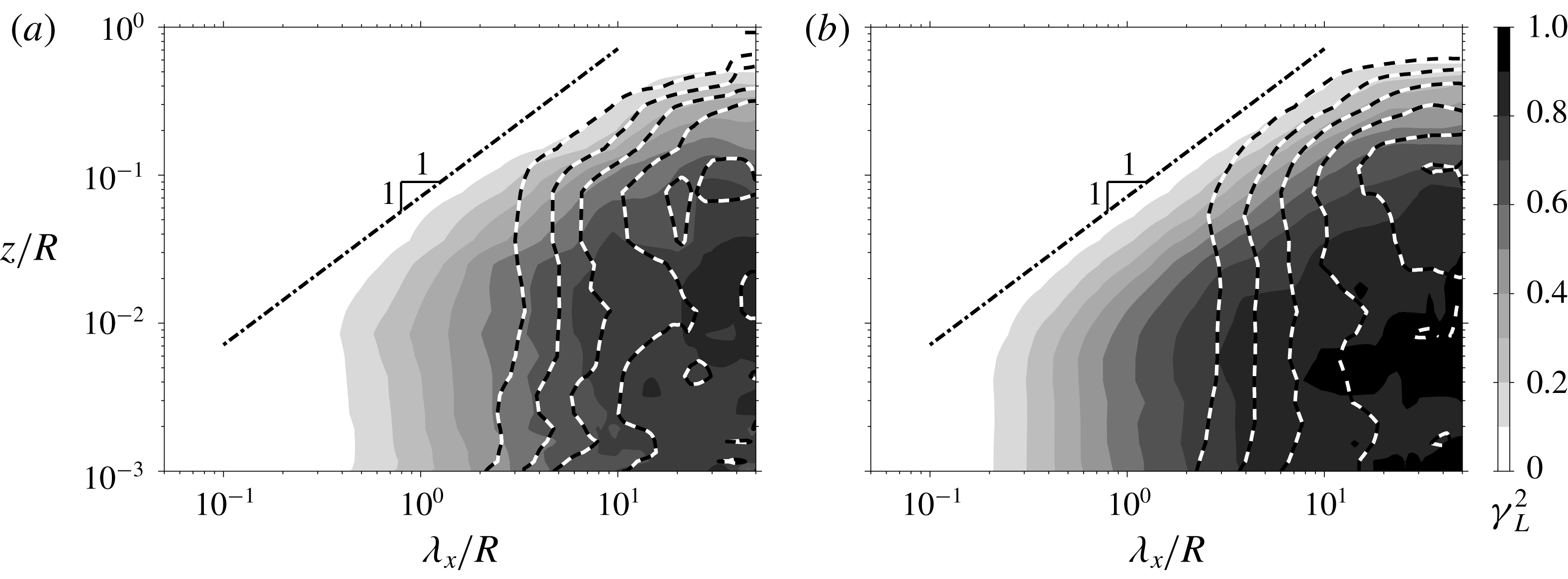
Value of $\unicode[STIX]{x1D6FE}_{L}^{2}$ for a pipe flow at (a) $Re_{\unicode[STIX]{x1D70F}}\approx 10\,000$ and (b) $Re_{\unicode[STIX]{x1D70F}}\approx 40\,000$ . The grey scale and line contours are as in figure 9.

4.2 Effects of Reynolds number

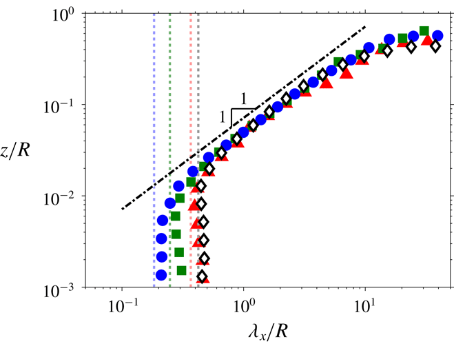
Figures 11(a) and 11(b) show the coherence spectra from the pipe flow at $Re_{\unicode[STIX]{x1D70F}}\approx 10\,000$ and 40 000, respectively. The grey scale and line contours again denote two transverse offset scenarios $\unicode[STIX]{x0394}s\approx 0$ and $\unicode[STIX]{x0394}s/R,\unicode[STIX]{x0394}s/\unicode[STIX]{x1D6FF}\approx 0.07$ , as in figure 9. Increasing $Re$ is accompanied by a larger scale separation between the viscous and inertial scales, and therefore also by an increase in the number of hierarchy levels required to model a wall-bounded flow. Indeed, this is reflected in an extended range of scales for which the $\unicode[STIX]{x1D6FE}_{L}^{2}=0.1$ iso-contours (for the $\unicode[STIX]{x0394}s\approx 0$ scenario) follow the $\unicode[STIX]{x1D706}_{x}\sim z$ scaling with increasing $Re$ for the pipe flows, as observed in figure 12. Also shown in figure 12 as vertical dotted lines are $\unicode[STIX]{x1D706}_{x}^{+}=A_{xz}\,z_{inertial}^{+}$ relations for each $Re$ case, where $z_{inertial}^{+}=2.6\sqrt{Re_{\unicode[STIX]{x1D70F}}}$ and $3.6\sqrt{Re_{\unicode[STIX]{x1D70F}}}$ for the pipe and boundary layer flows, respectively (Wei et al. Reference Wei, Fife, Klewicki and McMurtry2005; Morrill-Winter, Philip & Klewicki Reference Morrill-Winter, Philip and Klewicki2017). Here, $z_{inertial}$ corresponds to wall height where the mean viscous force first becomes sub-dominant in the mean momentum balance, and notably the $\unicode[STIX]{x1D6FE}_{L}^{2}=0.1$ iso-contours in the near-wall region closely align with the $\unicode[STIX]{x1D706}_{x}^{+}=A_{xz}\,z_{inertial}^{+}$ relation for both the pipe and boundary layer flows. Note that the $z$ -independent trend of $\unicode[STIX]{x1D6FE}_{L}^{2}$ iso-contours observed in the experiment is not present in the coherence spectra from DNS (Baars et al. Reference Baars, Hutchins and Marusic2017). Hence, the experiments are unable to capture the wall-attached structures that reside in the region $z<z_{inertial}$ . A potential cause for this is a small but finite spanwise misalignment that exists in the experiments between the skin friction and velocity sensors, which would lead to an attenuation of $\unicode[STIX]{x1D6FE}_{L}^{2}$ . A lower limit for the $\unicode[STIX]{x1D706}_{x}\sim z$ scaling in the $\unicode[STIX]{x1D6FE}_{L}^{2}=0.1$ iso-contours is indicative of the presence of different physical mechanisms of the wall-attached turbulence in the region close to the wall, which are not captured by the experiments. The current results suggest that these mechanisms are closely associated with an increased prominence of the viscous term in the mean momentum balance for the near-wall region (Wei et al. Reference Wei, Fife, Klewicki and McMurtry2005; Morrill-Winter et al. Reference Morrill-Winter, Philip and Klewicki2017). It should be noted that the theory associated with the mean momentum balance shows that the scales of motions in the inertial domain are proportional to $z$ , and thus the wall-distance scaling is an analytical result, rather than requiring assumptions as in AEH.

Unlike the $\unicode[STIX]{x0394}s\approx 0$ case, an extension in the range of $\unicode[STIX]{x1D706}_{x}$ values that remain coherent does not occur at $\unicode[STIX]{x0394}s/R,\unicode[STIX]{x0394}s/\unicode[STIX]{x1D6FF}\approx 0.07$ with $Re$ (e.g. dashed lines in figure 11 a,b). This behaviour can be related to the transverse offset remaining fixed in the outer scale for these datasets, and effectively acting as a low-pass filter based on the outer scale where scales smaller than the cutoff $\unicode[STIX]{x1D706}_{x}$ do not remain coherent. In other words, the range of scales that are coherent is fixed between $O(0.1R)$ and $O(R)$ for both cases, leading to coherent scales that are separated by a factor of $R/0.07R\sim O(10)$ regardless of $Re$ . Furthermore, for the large-scale contributions, the iso-contours in figure 11(a,b) shows good agreement, consistent with the AEH.

Figure 12.

The $\unicode[STIX]{x1D6FE}_{L}^{2}=0.1$ contours between $u$ and $u_{\unicode[STIX]{x1D70F}}$ signals at $\unicode[STIX]{x0394}s\approx 0$ for pipe and boundary layer flows. The symbols are as in figure 5, while the vertical dotted lines correspond to $\unicode[STIX]{x1D706}_{x}^{+}=A_{xz}\,z_{inertial}^{+}$ relations for each case.

Figure 13.

The $\unicode[STIX]{x1D6FE}_{L}^{2}=0.1$ contours between $u$ and $u_{\unicode[STIX]{x1D70F}}$ signals at $Re_{\unicode[STIX]{x1D70F}}\approx 40\,000$ as a function of $\unicode[STIX]{x0394}s$ ; $\unicode[STIX]{x0394}s/R\approx 0$ (◃), 0.02 (▿), 0.03 (♢), 0.06 (▵) and 0.13 (▹).

4.3 Effects of transverse offset

Figure 14.

Value of $\unicode[STIX]{x1D6FE}_{L}^{2}$ as a function of wavelength, $\unicode[STIX]{x1D706}_{x}$ , and hot-film sensor offset distances along the circumference, $\unicode[STIX]{x0394}s$ , for the pipe flow at $Re_{\unicode[STIX]{x1D70F}}\approx 40\,000$ . The grey scale and line contours correspond to coherence when the hot-wire is at $z/R\approx 0.01$ (▪) and 0.07 (▫) respectively, with the hot-film (●) at an azimuthal offset of $\unicode[STIX]{x0394}s$ . Both contours are at levels 0.1:0.1:0.9, while $\unicode[STIX]{x0394}s$ is shown in (a) linear and (b) logarithmic scale.

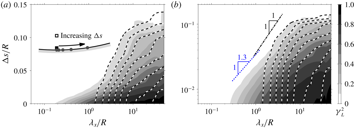
Figure 13 shows the effect of azimuthal offset $\unicode[STIX]{x0394}s$ for the $\unicode[STIX]{x1D6FE}_{L}^{2}=0.1$ iso-contours from $Re_{\unicode[STIX]{x1D70F}}\approx 40\,000$ pipe flow. An azimuthal offset between the $u_{\unicode[STIX]{x1D70F}}$ and $u$ sensors leads to a loss of common contributions encountered by the two sensors at the smaller scales since these scales do not span across the offset. Thus, a departure from the $\unicode[STIX]{x0394}s\approx 0$ contour occurs for any $\unicode[STIX]{x0394}s$ offsets larger than the width of the smallest attached eddy in the hierarchy, ${\mathcal{W}}_{1}$ , with the departure occurring at a higher $\unicode[STIX]{x1D706}_{x}$ when $\unicode[STIX]{x0394}s$ increases further.

To further assess the effect of transverse offset, figure 14 shows the coherence spectrum as a function of $\unicode[STIX]{x1D706}_{x}$ and $\unicode[STIX]{x0394}s$ . While figure 11(b) shows coherence spectra between a reference $u_{\unicode[STIX]{x1D70F}}$ and $u$ as the $z$ offset is varied, in figure 14 the $\unicode[STIX]{x0394}s$ offset (see inset, symbols ▪ and ●) is varied instead. Similar to figure 11(b), two scenarios are considered where now the grey scale and line contour correspond to cases when the $u$ sensor is at $z/R\approx 0.01$ and 0.07 respectively (see inset, symbols ▪ and ▫). It should also be noted that figure 14(a,b) are the same, except for $\unicode[STIX]{x0394}s$ being shown in linear and logarithmic scale, respectively. The iso-contours at $z/R\approx 0.01$ and $0.07$ agree well, at large $\unicode[STIX]{x1D706}_{x}$ and $\unicode[STIX]{x0394}s$ , while an increase in $z$ location where $u$ is acquired leads to a loss of coherence below a cutoff $\unicode[STIX]{x1D706}_{x}$ that scales with the distance from the wall. Furthermore, unlike figure 11(b) the iso-contours do not obey a $\unicode[STIX]{x1D706}_{x}\sim \unicode[STIX]{x0394}s$ (shown as dot-dashed line) scaling, even at $Re_{\unicode[STIX]{x1D70F}}\approx 40\,000$ , and instead $\unicode[STIX]{x1D706}_{x}\sim \unicode[STIX]{x0394}s^{1.3}$ behaviour is observed (shown as dotted line) for $\unicode[STIX]{x1D706}_{x}/R\sim O(1)$ and $\unicode[STIX]{x0394}s/R\sim O(0.01)$ . This is contrary to the AEH which predicts $\unicode[STIX]{x1D706}_{x}\sim \unicode[STIX]{x0394}s$ behaviour owing to eddy self-similarity and the wall scaling in both the $y$ and $z$ directions. The failure of $\unicode[STIX]{x1D706}_{x}\sim \unicode[STIX]{x1D706}_{y}$ behaviour has also been noted by del Álamo et al. (Reference del Álamo, Jiménez, Zandonade and Moser2004) who examined the two-dimensional spectra of $u$ from DNS. This failure, however, could be related to low $Re$ effects, as Chandran et al. (Reference Chandran, Baidya, Monty and Marusic2017) found evidence that the $\unicode[STIX]{x1D706}_{x}\sim \unicode[STIX]{x1D706}_{y}$ scaling may still emerge at the large scales at a higher $Re$ ( $Re_{\unicode[STIX]{x1D70F}}\sim O(10^{6})$ ) leading to an emergence of $\unicode[STIX]{x1D706}_{x}\sim \unicode[STIX]{x0394}s$ scaling for these scales. Hence, the current dataset at $Re_{\unicode[STIX]{x1D70F}}\approx 40\,000$ may not be sufficiently high to see the $\unicode[STIX]{x1D706}_{x}\sim \unicode[STIX]{x0394}s$ behaviour. Furthermore, similar to the $\unicode[STIX]{x1D706}_{x}\sim \unicode[STIX]{x1D706}_{y}$ scaling in the two-dimensional spectra, the $\unicode[STIX]{x1D706}_{x}\sim \unicode[STIX]{x0394}s$ scaling of $\unicode[STIX]{x1D6FE}_{L}^{2}$ contours are expected (at a sufficiently high $Re$ ) to first emerge at a $z$ location corresponding to the lower limit of the logarithmic region. This is because here the $u$ contributions from all hierarchy levels exist, while at a higher $z$ the contributions from hierarchy levels where ${\mathcal{H}}_{i}<z$ diminish. The dash-dotted line in figure 14 indicates $\unicode[STIX]{x1D706}_{x}=A_{xy}\unicode[STIX]{x0394}s$ , where $A_{xy}=28$ now is the predicted self-similar behaviour based on ${\mathcal{H}}_{i}={\mathcal{W}}_{i}$ (i.e. $A_{xy}=2A_{xz}$ since $z|_{\unicode[STIX]{x1D6FE}_{L}^{2}=\unicode[STIX]{x1D6E4}}=2\unicode[STIX]{x0394}s|_{\unicode[STIX]{x1D6FE}_{L}^{2}=\unicode[STIX]{x1D6E4}\,}$ , see figure 10). Furthermore, since $\unicode[STIX]{x1D706}_{x}$ is expected to be twice as large as the region of streamwise coherence ${\mathcal{L}}_{\,i}$ (see figure 10 a), this leads to an aspect ratio of $7:1:1$ for the self-similar eddy in the $x$ , $y$ and $z$ directions, respectively. It has to be noted that Krug et al. (Reference Krug, Baars, Hutchins and Marusic2019) found a clear dependence of this aspect ratio on the level of stratification, via analysis of atmospheric surface layer data. For our adiabatic wall case, the aspect ratio agrees well with the dimensions of attached eddies found in DNS, while the streamwise extent is slightly longer than that typically reported from DNS (Hwang Reference Hwang2015; del Álamo et al. Reference del Álamo, Jiménez, Zandonade and Moser2006). However, the value obtained for the streamwise extent of the attached eddies is consistent with the observation of Chandran et al. (Reference Chandran, Baidya, Monty and Marusic2017) that at a comparable $Re$ an energetic ridge in the two-dimensional $u$ -spectra follow an aspect ratio of $7:1$ in the $x$ and $y$ directions.

4.4 Extending the model of Baars et al.

Figure 15(a–d) shows a model for $\unicode[STIX]{x1D6FE}_{L}^{2}$ based on results shown in §§ 4.1–4.3 and following the AEH. In (a), $\unicode[STIX]{x1D6FE}_{L}^{2}$ as a function of both $\unicode[STIX]{x1D706}_{x}$ and $z$ is shown at a constant $\unicode[STIX]{x0394}s$ , and hence the contours at the lower value of $\unicode[STIX]{x0394}s$ where $\unicode[STIX]{x0394}s\approx 0$ is equivalent to the model of Baars et al. (Reference Baars, Hutchins and Marusic2017). In this model, the contribution to $\unicode[STIX]{x1D6FE}_{L}^{2}$ from each hierarchy level remains uniform across $\unicode[STIX]{x1D706}_{x}>A_{xz}{\mathcal{H}}_{i}$ . The hierarchy scaling prescribed by the AEH, ${\mathcal{H}}_{i}\sim 2^{(i-1)}{\mathcal{H}}_{1}$ , leads to a triangular region in the $\unicode[STIX]{x1D6FE}_{L}^{2}$ iso-contours bounded by $A_{xz}{\mathcal{H}}_{1}\lesssim \unicode[STIX]{x1D706}_{x}\lesssim A_{xz}{\mathcal{H}}_{N_{H}}$ . Here $N_{H}$ denotes the number of hierarchy levels used in the model, which is $Re$ dependent (e.g. $N_{H}=4$ , for the examples shown in figures 8 and 15 a–c). When $\unicode[STIX]{x0394}s>0.5{\mathcal{W}}_{1}$ , the lower bound of the triangular region increases, since an $i$ th hierarchy level with width ${\mathcal{W}}_{i}<2\unicode[STIX]{x0394}s$ does not remain coherent across the two points, leading to $\unicode[STIX]{x1D6FE}_{L}^{2}\approx 0$ at the smaller scales as shown in figure 15(a).

Figure 15.

A model for $\unicode[STIX]{x1D6FE}_{L}^{2}$ following the attached eddy hypothesis. (a–c) Correspond to the case with four hierarchy levels, with (a) and (b) showing $\unicode[STIX]{x1D6FE}_{L}^{2}$ at a constant $\unicode[STIX]{x0394}s$ and $z$ , while (c) illustrates the iso-contours of $\unicode[STIX]{x1D6FE}_{L}^{2}$ as functions of $\unicode[STIX]{x1D706}_{x}$ , $\unicode[STIX]{x0394}s$ and $z$ . Meanwhile, (d) shows the iso-contours for the case with ten hierarchy levels, which corresponds to a higher $Re$ scenario.

Figure 15(b) shows $\unicode[STIX]{x1D6FE}_{L}^{2}$ as a function of $\unicode[STIX]{x0394}s$ and $\unicode[STIX]{x1D706}_{x}$ at a constant $z$ . Although the $\unicode[STIX]{x1D706}_{x}\sim \unicode[STIX]{x0394}s$ scaling indicated in the figure did not materialise for the experimental data, evidence points towards its emergence at sufficiently high $Re$ , when $Re_{\unicode[STIX]{x1D70F}}\sim O(10^{6})$ (Chandran et al. Reference Chandran, Baidya, Monty and Marusic2017). Thus in the asymptotic limit, the hierarchy of eddies are expected to be truly self-similar (i.e. the wall scaling holds in all three directions – $x$ , $y$ and $z$ ), and therefore we expect a triangular region for the $\unicode[STIX]{x1D6FE}_{L}^{2}$ contours in the $\unicode[STIX]{x1D706}_{x}$ – $\unicode[STIX]{x0394}s$ plane in an analogous manner to the $\unicode[STIX]{x1D706}_{x}$ – $z$ plane. Furthermore, the triangular region through this slice is now bounded by $A_{xz}{\mathcal{W}}_{1}\lesssim \unicode[STIX]{x1D706}_{x}\lesssim A_{xz}{\mathcal{W}}_{N_{H}}$ (since ${\mathcal{H}}_{i}\sim {\mathcal{W}}_{i}$ ) when $z<{\mathcal{H}}_{1}$ , since contributions to $\unicode[STIX]{x1D6FE}_{L}^{2}$ from all hierarchy levels are captured at those locations (see figure 15 b at a lower $z$ location). Beyond this wall height, the lower bound of the triangular region increases due to loss of coherence from the smaller members of the hierarchy.

Combining the results from figure 15(a,b), figure 15(c) depicts the full three-dimensional picture of $\unicode[STIX]{x1D6FE}_{L}^{2}$ contours as a function of $\unicode[STIX]{x1D706}_{x},\unicode[STIX]{x0394}s$ and $z$ . Here, the triangular regions observed on constant $\unicode[STIX]{x0394}s$ and $z$ planes now correspond to the face of a skewed pyramid, as eddies that do not meet the ${\mathcal{W}}_{i}>2\unicode[STIX]{x0394}s$ and ${\mathcal{H}}_{i}>z$ criteria do not remain coherent over the two points used to calculate $\unicode[STIX]{x1D6FE}_{L}^{2}$ . At a higher $Re$ , the number of hierarchy levels required in the model increases, leading to a more extended pyramidal region for the $\unicode[STIX]{x1D6FE}_{L}^{2}$ iso-contours as shown in figure 15(d).