


A variable that has received considerable attention in studies of early vocabulary development is phonological neighbourhood density, commonly defined as the number of words in a given corpus that can be formed by the addition, substitution, or elimination of a single phoneme in a target word (e.g., cat neighbours catch, mat, and at; Luce & Pisoni, Reference Luce and Pisoni1998; e.g., Storkel, Reference Storkel2004; Storkel & Lee, Reference Storkel and Lee2011; Stokes, Reference Stokes2010, Reference Stokes2014; Stokes, Kern, & Dos Santos, Reference Stokes, Kern and Dos Santos2012; Takac, Knott, & Stokes, Reference Takac, Knott and Stokes2017). Work in this direction suggests that words with high phonological neighbourhood density – i.e., words that sound similar to many other words in the target language – may be learned developmentally earlier, and on fewer experimental exposures, than words that are phonologically similar to few other words. Prominent causal accounts of this effect maintain that high neighbourhood density words contain regularly occurring sounds that are held in memory more accurately during short-term processing (e.g., the at in cat, mat, and catch; Gathercole, Frankish, Pickering, & Peaker, Reference Gathercole, Frankish, Pickering and Peaker1999), and that this supports the formation of highly detailed long-term word memory traces (Hoover, Storkel, & Hogan, Reference Hoover, Storkel and Hogan2010; Metsala & Walley, Reference Metsala, Walley, Metsala and Ehri1998; Sosa & Stoel-Gammon, Reference Sosa and Stoel-Gammon2012; Storkel, Reference Storkel2004; Walley, Metsala, & Garlock, Reference Walley, Metsala and Garlock2003).
Previous studies reporting high neighbourhood density advantages in early word learning have, however, considered neighbourhood density alongside only a small number of alternative predictor variables, most notably word frequency, length, and phonotactic probability (i.e., the positional probabilities of adjacent phonemic segments) (e.g., Storkel, Reference Storkel2004; Stokes, Reference Stokes2014). This is unsatisfactory because properties that appear to facilitate word acquisition in relative isolation may prove to have only a limited impact when considered alongside a more representative range of explanatory variables. For instance, Braginsky, Yurovsky, Marchman, and Frank (Reference Braginsky, Yurovsky, Marchman and Frank2018) report that word valence and word arousal, semantic features identified by Moors et al. (Reference Moors, De Houwer, Hermans, Wanmaker, Van Schie, Van Harmelen and Brysbaert2013) as important determinants of word acquisition, have a relatively limited effect when modelled as part of a more representative set of predictors.
The work of Braginsky and colleagues (Braginsky, Yurovsky, Marchman, & Frank, Reference Braginsky, Yurovsky, Marchman and Frank2016; Braginsky et al., Reference Braginsky, Yurovsky, Marchman and Frank2018) – an important impetus for the current study – predicted age of acquisition for words using word frequency, word length, and a range of semantic variables (including valence and arousal) that are fully defined below. In doing so, these authors have provided the most comprehensive survey to date of features linked to effects in early word learning. Braginsky et al. (Reference Braginsky, Yurovsky, Marchman and Frank2016, Reference Braginsky, Yurovsky, Marchman and Frank2018) acknowledge, however, that their explanatory models of early word learning are incomplete, with a substantial proportion of variance left unexplained (estimated at R 2 = 71% in Braginsky et al., Reference Braginsky, Yurovsky, Marchman and Frank2016). The purpose of the current study is to build on Braginsky and colleagues’ work by asking: When adopting a similar multi-predictor methodology, how much does word sound matter in early word learning? The variable of primary interest in this study is phonological neighbourhood density, which, as outlined above, has been widely studied in child language research. Research Question 1 asks:
What is the strength of association between phonological neighbourhood density and word understanding and word production when neighbourhood density is modelled alongside a representative inventory of predictor variables?
Following previous analyses by Braginsky et al. (Reference Braginsky, Yurovsky, Marchman and Frank2016, Reference Braginsky, Yurovsky, Marchman and Frank2018), the current study also examines developmental changes in the importance of phonological neighbourhood density and control variables as predictors of word understanding and production. Research Question 2 asks:
Do phonological neighbourhood density and other predictors interact with age to affect word understanding and word production?
Method
This study was pre-registered with the Open Science Framework on 16 September 2018. A pre-registration protocol, R code, and all data required to re-run the analyses are available via the associated project page <https://osf.io/zfy2p/>.
Dependent variables
We used communicative development inventory (CDI) data to examine phonological neighbourhood density effects in early word learning. The common format of a communicative development inventory is a wordlist plus checkboxes with fixed response options. For instance, the word cat may be listed as one of many words, each with two response options: ‘understands’ and ‘produces’. During administration, caregivers may check the first box if the target child is able to understand the word cat, and check the second box if the target child is able to produce the word cat. The dependent variables used in the current study were ‘understands’ and ‘produces’ responses to 418 words from the Oxford Communicative Development Inventory, accessed via the Stanford Wordbank project (Frank, Braginsky, Yurovsky, & Marchman, Reference Frank, Braginsky, Yurovsky and Marchman2017; Hamilton, Plunkett, & Schafer, Reference Hamilton, Plunkett and Schafer2000). Following previous work by Braginsky and colleagues, we restricted our analysis to cross-sectional responses. This data, collected by Floccia (Reference Floccia2017) over a five-year period at Plymouth University, contains responses from caregivers of 300 British English-speaking children (n = 140 female) between the ages of 12 and 25 months (M = 18.61 months).
Parental report data are subject to reasonable validity concerns, with respondents potentially over- or under-reporting the linguistic knowledge of target children, and such biases potentially affecting modelling results (see Bennetts, Mensah, Westrupp, Hackworth, & Reilly, Reference Bennetts, Mensah, Westrupp, Hackworth and Reilly2016, for review). One anonymous reviewer commented that parental report comprehension data may be particularly noisy. However, the cost of administering communicative inventories is low, meaning – as Braginsky et al. (Reference Braginsky, Yurovsky, Marchman and Frank2018) note – that sample sizes are often large enough to reduce the impact of noise at the individual respondent level. The advantages of parental report data are that they provide insight into the linguistic knowledge of the child as realised in a naturalistic setting during talk with familiar people; they assess a number of words way in excess of the typical stimulus count in an experimental design; and they provide an index of words both understood and produced, allowing researchers to assess how different lexical characteristics affect these different aspects of early word learning.
Independent variables
Braginsky et al. (Reference Braginsky, Yurovsky, Marchman and Frank2016, Reference Braginsky, Yurovsky, Marchman and Frank2018) present an inventory of independent variables previously assessed with respect to their association with word acquisition. The authors’ approach follows Goodman, Dale, and Li (Reference Goodman, Dale and Li2008) in appropriating predictor data from multiple sources. We broadly adopted Braginsky et al.’s (Reference Braginsky, Yurovsky, Marchman and Frank2016, Reference Braginsky, Yurovsky, Marchman and Frank2018) inventory of predictor variables, although we made changes to certain data sources (see Table 1) and excluded predictors related to sentence complexity, such as a word's mean length of utterance or utterance position frequency, in order to home in on lexical effects. We then built on Braginsky et al.’s inventory by incorporating ambient language phonological neighbourhood density. Predictors, associated data sources, and example words are shown in Table 1.
Independent variables, data sources, and minimum and maximum value examples from the Oxford CDI data

The log child-directed speech frequency of each word was calculated from caregiver utterances in the Manchester corpus, which is hosted within the CHILDES database (MacWhinney, Reference MacWhinney2000; Theakston et al., Reference Theakston, Lieven, Pine and Rowland2001). This corpus includes transcripts from 12 typically developing English-speaking children (age range 1;8.22–2;0.25 at study onset) and their caregivers, who were recorded in free play for one hour, twice every three weeks for one year. Collectively these transcripts comprised 1,454,060 child-directed word tokens and 12,734 child-directed word types. Phoneme counts for each CDI word were retrieved from the English Lexicon Project (Balota et al., Reference Balota, Yap, Cortese, Hutchison, Kessler, Loftis and Treiman2007), with diphthongs and affricates counted as single phonemes. The English Lexicon Project provides lexical characteristic data for 40,481 words, including behavioural measures (response times and accuracy) from 1,200 subjects. Other commonly used measures of word length, including number of orthographic letters, syllables, or morphemes, are closely correlated, and may therefore provide similar results (e.g., as in Lewis & Frank, Reference Lewis and Frank2016). We selected the phoneme-based measure of word length given the central interest in the phoneme as a unit of representation in the current analysis (i.e., as the basis of similarity neighbourhoods). Multiple data sources were accessed to retrieve adult ratings for babiness, concreteness, valence, arousal, and dominance. Babiness refers to the relevance of a word to babies and infants; concreteness refers to word tangibility versus abstractness; valence refers to associations with happiness or sadness; arousal to degree of excitability; and dominance to whether the word invokes notions of being controlled or submissive, or being in control or strong. Note that this last variable, dominance, was not included in prior studies by Braginsky et al. (Reference Braginsky, Yurovsky, Marchman and Frank2016, Reference Braginsky, Yurovsky, Marchman and Frank2018). We include this variable here because it has been associated with age-related interactions in previous studies, with early learned words having relatively high dominance ratings (Brysbaert et al., Reference Brysbaert, Warriner and Kuperman2014). Finally, plus-minus-one phoneme phonological neighbourhood densities for each Oxford CDI word were retrieved from the English Lexicon Project (Balota et al., Reference Balota, Yap, Cortese, Hutchison, Kessler, Loftis and Treiman2007). We should acknowledge that there are a number of alternative measures of word-level phonological similarity. For instance, similarity may be calculated across only word onsets, or by taking the average edit distance between the target word and that word's twenty nearest neighbours (i.e., PLD20; Suárez, Tan, Yap, & Goh, Reference Suárez, Tan, Yap and Goh2011). We selected the un-weighted plus-minus-one phoneme measure of phonological neighbourhood density excluding homophones because this is the most commonly used criterion in the developmental literature, plausibly due to the long-term dominance of this measure in adult word recognition and production studies (e.g., Storkel, Reference Storkel2004; Storkel & Lee, Reference Storkel and Lee2011; Stokes, Reference Stokes2010, Reference Stokes2014; Stokes et al., Reference Stokes, Kern and Dos Santos2012; Takac et al., Reference Takac, Knott and Stokes2017). Importantly, this consistency allows us to directly re-evaluate the existing developmental literature reporting high neighbourhood density word learning advantages in the context of a big data, multiple-predictor analysis. Given the strong correlation between different measures of word-level phonological similarity (Suárez et al., Reference Suárez, Tan, Yap and Goh2011), we would expect the results reported below to hold across alternative measures.
It is also important to acknowledge word sound variables other than phonological neighbourhood density. Given our central interest in neighbourhood density effects, we omitted alternative measures including phonological variability (i.e., the degree to which productions of a single word by a single speaker vary) and phonotactic probability, which was omitted because high correlation with neighbourhood density would have caused multicollinearity (Storkel & Lee, Reference Storkel and Lee2011; see ‘Missing data and multicollinearity’ below for further discussion of this issue). It is likely, however, that experimenting with alternative word sound variables within a similar multi-predictor framework will improve current understanding of the factors that facilitate early word learning. Readers are therefore invited to use our data to experiment with different configurations of predictor variables, for instance by including alternative measures of neighbourhood density (e.g., PLD20) or variables such as phonotactic probability (the data repository can be found at <https://osf.io/zfy2p/>).
Missing data and multicollinearity
The percentage of missing data ranged from 0% to 22.73% across predictor variables (see ‘Appendix A’ for rates of missing data, predictor correlations, and variance inflation factors). We imputed missing values using predictive mean matching via the mice (multivariate imputation by chained equations) package in R (Buuren & Groothuis-Oudshoorn, Reference Buuren and Groothuis-Oudshoorn2010; R Core Team, 2016). All predictors were then centred and scaled into comparable units (i.e., M = 0, SD = 1).
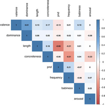
Figure A1 in ‘Appendix A’ shows substantial correlations between word length and phonological neighbourhood density (r = –0.66), as well as between word valence and dominance (r = 0.61), and concreteness and frequency (r = –0.51). Multicollinearity risk was assessed by fitting a multivariate binomial multiple regression model and computing variance inflation factors (VIFs) using the lme4 and car packages in R (Bates, Maechler, Bolker, & Walker, Reference Bates, Maechler, Bolker and Walker2015; Fox & Weisberg, Reference Fox and Weisberg2011). Estimates suggested multicollinearity risk was low across predictors, with a maximum value of VIF = 1.93 for the word length variable. We also conducted a post-hoc sensitivity analysis, in which we removed the word length variable and refitted the Bayesian regression model introduced fully below (see ‘Model fitting’). Word length was selected for removal in this analysis because of its relatively high VIF and correlation with neighbourhood density, which was the primary independent variable of interest. We found no substantial difference in estimates from the model including word length and the model excluding word length, in terms of the direction or magnitude of the estimates, or the size of the estimate errors. This can be confirmed by recalling the model summaries using the R code associated with this project, available from <https://osf.io/zfy2p/>.
Model fitting
We used the brms package (Bürkner, Reference Bürkner2017) to fit a Bayesian multivariate multiple binomial regression model. The model specified two outcome variables; (i) understands and (ii) produces, as reported in the 418-item communicative inventory data from 300 children. Outcomes were configured as the proportion of children at each month of age (i.e., 12 to 25 months; a 14-month range) who were able to understand or produce each item. Therefore there were 14 × 418 = 5852 rows of data. Word understanding and production were predicted by the independent variables listed in Table 1 both as main effects and in interaction with the age of the target child at the time of communicative inventory completion. We specified a random slope for age for each word, a binomial family likelihood, and a weakly informative prior across beta parameters. This model fitted successfully, with a sufficient number of effective samples, stationery and well-mixing chains, no rhats above 1.1, and credible posterior predictive checks. These analytics can be confirmed by recalling the model summary in the R code associated with this project at <https://osf.io/zfy2p/>.
Results
Model summaries are shown in ‘Appendix B’. Main effects can be seen in Figure 1, where the estimated strength of association between each predictor and outcome variable is visualised as a probability distribution. A distribution with mass below zero indicates a negative association between variables; a distribution with mass above zero indicates a positive association between variables; and a probability distribution centred on zero suggests no relationship between variables.
Estimate probability masses for each predictor variable in the inventory, split by understands and produces outcomes. The central vertical line is the estimate mean, the shaded region is the 50% probability interval, and the distribution tails cover the 99% probability region. Positive values indicate that learned words were, on average, high in the associated variable. Negative values indicate that learned words were, on average, low in the associated variable. PND indicates phonological neighbourhood density.

Words that children both understood and produced typically occurred at high frequency in the corpus of child-directed speech (e.g., you, it, and that). While many children understood relatively long words (e.g., cock-a-doodle-do, pushchair, and television), they tended to produce words with relatively few phonemes (e.g., no, yes, hi, bye, and ball). Words children both understood and produced scored highly on adult ratings of babiness (e.g., bottle, milk, and blanket) and concreteness (e.g., doll, ball, and fish). The direction of effects for word valence, arousal, and dominance differed by outcome measure. Positive valence (e.g., happy, hug, and love) and positive arousal (e.g., chase, naughty, and spider) were negatively associated with understanding but positively associated with production. In contrast, high dominance (e.g., smile, happy, help) was positively associated with word understanding and negatively associated with production. Finally, and with central importance to the current study, the estimate probability mass for phonological neighbourhood density (PND) was centred on zero for understanding, but positive for word production. This suggests that, when we have already taken into account a word's frequency, length, babiness, concreteness, valence, arousal, and dominance, additionally knowing that word's phonological neighbourhood density does little to improve the prediction of early word understanding, but does improve the prediction of early word production. The children assessed were more likely to produce words that were phonologically similar to many other words in the language to which they were exposed (e.g., toe, show, shoe, bee, and key).
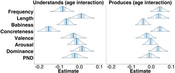
Figure 2 shows interactions between each predictor and participant age, which ranged between 12 and 25 months. A positive interaction estimate indicates that the value of the predictor became more positive as age increased (e.g., a slope estimate increase from 0.01 to 0.03 between 12 and 25 months). A negative interaction estimate indicates that the value of the predictor became more negative as age increased (e.g., a slope estimate decrease from 0.01 to –0.01 between 12 and 25 months). An interaction estimate centred on zero suggests no change in the value of the predictor with age. Note that the interpretation of interaction effects depends on the direction (or sign) of the main effect. For instance, if the sign of the main effect is positive, a positive interaction with age indicates a strengthening of this effect (e.g., an increase from 0.01 to 0.03). However, if the sign of the main effect is negative, a positive interaction with age may indicate a weakening of this negative effect (i.e., a negative effect approaching zero as age increases; e.g., from –0.03 to 0).
Predictor-age interaction effect probability masses by outcome. The central vertical line is the estimate mean, the shaded region is the 50% probability interval, and the distribution tails cover the 99% probability region. Positive values indicate that the value of the predictor became more positive as age increased from 12 to 25 months. Negative values indicate that the value of the predictor became more negative between 12 and 25 months. PND indicates phonological neighbourhood density.

High input frequency became a less important determinant of word understanding across development. However, children became increasingly able to produce the words they were exposed to most frequently (e.g., you, it, and that). Older children were able to understand and produce words comprising more phonemes than younger children (e.g., cock-a-doodle-do, pushchair, and television). High relevance to the lives of babies and infants became a less important predictor of word understanding and production between 12 and 25 months, with older children acquiring low relevance words such as broom, scissors, and write. The association between concreteness and understanding weakened with age, as children learned abstract words such as how, later, and bad. But the association between concreteness and production increased over development, with words such as knee, bird, and comb becoming part of the children's productive vocabularies. Negative trends were seen for both valence and (marginally) arousal across development, with older children more likely to understand and produce words such as sad, sick, and hurt (low valence), and asleep, tea, and blanket (low arousal). Dominance became more positively associated with understanding and less negatively associated with production (i.e., the production estimate approached zero; see Figure 1). That is, older children were more likely to understand and produce words with associations of being in control (e.g., smile, happy, help, eat, and say).
For both understands and produces outcomes, the phonological neighbourhood density (PND) estimate was marginally negative, suggesting that phonological similarity to other words in the language to which children are exposed became a weaker determinant of word understanding and production across development. Estimates suggest that, at around 12 months, children are more likely to produce words that sound similar to other words they hear (e.g., toe, show, shoe, bee, and key), but that by 25 months they are able to both understand and produce words comprising less frequent sound sequences (e.g., breakfast, telephone, toothbrush, and trousers).
Discussion
In this study, we estimated the strength of the association between phonological neighbourhood density and word understanding and production when a wide range of other determining factors, including word frequency, length, valence, concreteness, babiness, arousal, and dominance, were taken into account. We also examined whether the importance of phonological neighbourhood density as a predictor of word understanding and production changed between the ages of 12 and 25 months. Results broadly comparable with prior research were observed where predictor inventories overlapped. Early learned words were, for instance, high in child-directed speech frequency (for understanding and production), short in length (for production only), and high in babiness rating (for understanding and production) (Braginsky et al., Reference Braginsky, Yurovsky, Marchman and Frank2016, Reference Braginsky, Yurovsky, Marchman and Frank2018). Interaction effects also showed close parallels with prior work. A word's association with babies, for instance, was a more important predictor of word understanding and production early in development than it was late in development (Braginsky et al., Reference Braginsky, Yurovsky, Marchman and Frank2016, Reference Braginsky, Yurovsky, Marchman and Frank2018).
Our estimates suggest that phonological neighbourhood density is an important predictor of early word production though not word understanding. In understanding a word, the balance of importance across the predictors assessed favoured high frequency of exposure, high concreteness, and high relevance to the lives of babies and infants. A word with such characteristics but complex phonology may be memorised imperfectly, which may be sufficient if the child is required to recognise and respond to, though not necessary produce, such a word (e.g., “Eat your breakfast!” “Do you want to rest in the pushchair?” “Where's your toothbrush?”). However, accurate production is impossible with imperfect phonological memorisation. Therefore, with respect to word production there is an increase in the relative importance of high phonological neighbourhood density, and concurrently shorter word length (in phonemes). That is, words enter the productive lexicon more readily if their phonology is easy to remember, in terms of a low number of phonemes that occur frequently in the language to which children are exposed.
Estimates for the interaction between neighbourhood density and age suggest that phonological similarity to other words in the ambient language is a more important predictor of word understanding and production early in development rather than late in development. These results accord closely with those of prior studies reporting that the importance of phonological neighbourhood density as a predictor of word acquisition is greater in younger children and children with language delay, particularly with respect to word production (e.g., Storkel, Reference Storkel2004; Storkel & Lee, Reference Storkel and Lee2011; Stokes, Reference Stokes2010, Reference Stokes2014; Stokes et al., Reference Stokes, Kern and Dos Santos2012; Takac et al., Reference Takac, Knott and Stokes2017). It is plausible that this effect signals increased competence in phonemic and word-level phonological representation. Accurately representing phonologically anomalous words may be difficult in early development given a relatively low frequency of exposure and limited production practice. As a result, young children may tend implicitly towards acquiring new words comprising familiar phonological patterns. Later in development, however, children are better able to represent a wider range of sounds, making phonological neighbourhood density a marginally less important predictor of whether or not a word is acquired.
A prominent explanatory account of the high neighbourhood density advantage is that cognitive demand is low during the initial processing of a novel spoken word comprising commonly occurring sounds, and that this enables the formation of detailed long-term phonological word memories that are relatively robust to forgetting and which provide detailed motor plans supporting accurate word production (Gathercole et al., Reference Gathercole, Frankish, Pickering and Peaker1999; Hoover et al., Reference Hoover, Storkel and Hogan2010; Metsala & Walley, Reference Metsala, Walley, Metsala and Ehri1998; Sosa & Stoel-Gammon, Reference Sosa and Stoel-Gammon2012; Storkel, Reference Storkel2004; Walley et al., Reference Walley, Metsala and Garlock2003). A limitation of the current study is that it is impossible to provide evidence for any causal account on the basis of correlational data alone. In fact, it has proven difficult to test explanatory accounts of the density advantage even in tightly controlled experiments, given, for instance, multicollinearity between different word sound metrics such as neighbourhood density and phonotactic probability. The early high-density word learning advantage is, however, non-trivial, with a substantial literature documenting memorisation advantages for phonologically distinctive (i.e., as opposed to similar, or dense) stimuli (see Hunt & Worthen, Reference Hunt and Worthen2006, for a review), and further work is required to develop the causal account of this phenomenon. What the current study shows is that any explanatory model of early vocabulary development, particularly of early word production, must account for word sound features.
Acknowledgements
This study was unfunded and undertaken as part of the first author's PhD. We declare no conflicts of interest. Thank you to Paul-Christian Bürkner at the University of Münster for his advice on model fitting using the brms package.
Appendix A
Predictor correlations, rates of missing data, and variance inflation factors (VIFs)
Post-imputation Pearson correlations between predictors (pnd indicates phonological neighbourhood density).

Rates of missing data and variance inflation factors for each predictor variable, calculated (using the car and lme4 packages in R) from the model: glmer(cbind(understands, produces) ~ length + pnd + frequency + babiness + concreteness + valence + arousal + dominance + (1 | word), family = binomial). Note that VIFs are shown for post-imputation values.

Appendix B
Model summaries
Model summary for the understands outcome, showing term, estimate, standard error (Std. error), and lower and upper 95% confidence intervals (CI). CDS indicates child-directed speech. PND indicates phonological neighbourhood density.

Model summary for the produces outcome, showing term, estimate, standard error (Std. error), and lower and upper 95% confidence intervals (CI). CDS indicates child-directed speech. PND indicates phonological neighbourhood density.