


1. Introduction
The equation of exchange,
 $M_{t}V_{t}=P_{t}Y_{t}$
, where
 $M_{t}$
is the total amount of money in the economy,
 $V_{t}$
the velocity of money (the number of times money gets used in period
 $t$
),
 $P_{t}$
the price level, and
 $Y_{t}$
real output, is a foundation of monetarist theory. It is an accounting identity according to which total dollar spending on the economy, or nominal gross domestic product (GDP),
 $M_{t}V_{t}$
, equals total dollar income, or nominal gross domestic income,
 $P_{t}Y_{t}$
. Assuming that velocity is fairly constant in the short run, that
 $Y_{t}$
is at the full employment level, and that
 $M_{t}$
is exogenous, transforms the equation of exchange into the quantity theory of money. The quantity theory of money has been the primary theory of price level (and inflation) determination, and states that the price level,
 $P_{t}$
, is solely determined by the quantity of nominal money balances,
 $M_{t}$
, as
 $P_{t}=M_{t}V_{t}/Y_{t}$
.
The velocity of money,
 $V_{t}$
, is central to the quantity theory of money and for understanding the dynamic relationship between the money supply, inflation, and economic output. In fact, whether velocity is stable or at least predictable is essential to any empirical interpretation of the monetarist position and especially relevant for some problems of potential importance in the practical conduct of monetary policy. For these reasons, a substantial amount of attention has been focused on the behavior of the velocity of money in the United States, primarily as the result of a relatively sudden and unanticipated decline in the velocity series in 1981 and in more recent economic downturns, such as the 2008 financial crisis and the Covid-19 pandemic. The most powerful element of these statistically unusual declines in velocity is the collapse of the long-run relationship connecting money to both income and prices.
The debate that has arisen mostly concerns a few specific hypotheses regarding the determinants of the velocity of money. Among the propositions advanced, those most often cited involve the influence of large and permanent shifts arising from financial innovation and changes in regulation, tax cuts, inflation (or expected inflation), changes in government expenditures, changes in energy prices, and money growth along with its variability—see especially Tatom (Reference Tatom1983), Judd and Motley (Reference Judd and Motley1984), Hall and Noble (Reference Hall and Noble1987), Santoni (Reference Santoni1987), and Fisher and Serletis (Reference Fisher and Serletis1989), Serletis and Shahmoradi (Reference Serletis and Shahmoradi2006), Anderson et al. (Reference Anderson, Bordo and Duca2017), Bordo and Duca (Reference Bordo and Duca2025), Bordo et al. (Reference Bordo, Duca and Jones2025), and Chowdhury and Serletis (Reference Chowdhury and Serletis2025) for more on these and other suggested (and sometimes empirically supported) influences.
In this paper we explore the variability of money growth as an influence on the velocity of money. In this regard, Friedman (Reference Friedman1983, Reference Friedman1984) proposed two avenues of influence of the variability of money growth on velocity. The first involves the behavior of real income and the second concerns the behavior of the demand for money (accommodated by money supply). Regarding the real income effect, although Friedman’s position is not precisely stated, the idea is that an increase in monetary variability creates greater uncertainty and instability in real incomes, which in turn increases the responsiveness of money demand to changes in real economic activity. As a result, fluctuations in real income have a larger impact on the demand for money balances, making the velocity of money more sensitive to changes in real economic conditions. Regarding the money demand effect, Friedman argued that increased uncertainty in financial markets, because of increased volatility of money, produces both an increased demand for money for (essentially) precautionary purposes and, assuming that the money supply process accommodates the pressure, a rise in money holdings relative to nominal income. Thus, the equilibrium stock of money increases and velocity declines with increases in the volatility of money growth.
We investigate the Friedman hypothesis, extending the works of Hall and Noble (Reference Hall and Noble1987), Brocato and Smith (Reference Brocato and Smith1989), Fisher and Serletis (Reference Fisher and Serletis1989), Thornton (Reference Thornton1995), and Serletis and Shahmoradi (Reference Serletis and Shahmoradi2006). These authors, with the exception of Serletis and Shahmoradi (Reference Serletis and Shahmoradi2006), use moving (sample) standard deviations of money growth rates to measure the variability of money growth and the Granger-causality method to test the general hypothesis that the variability of money growth causes velocity to change. Serletis and Shahmoradi (Reference Serletis and Shahmoradi2006) estimate a bivariate VARMA GARCH-in-Mean model of money growth and velocity growth, using quarterly data from 1959:1 to 2004:3 and the St. Louis Federal Reserve Monetary Services Index database. In contrast to Brocato and Smith (Reference Brocato and Smith1989), Mehra (Reference Mehra1989), and Thornton (Reference Thornton1995), they find evidence of Friedman’s hypothesis that the variability of money growth helps predict velocity.
We use standard Granger causality tests, as in Hall and Noble (Reference Hall and Noble1987), Brocato and Smith (Reference Brocato and Smith1989), Fisher and Serletis (Reference Fisher and Serletis1989), and Thornton (Reference Thornton1995). For the first time, we also use a bivariate (identified) structural GARCH-in-Mean VAR model, introduced by Elder (Reference Elder2004) to investigate the macroeconomic effects of inflation uncertainty and also used by Elder and Serletis (Reference Elder and Serletis2010) in their investigation of the effects of oil price uncertainty. This is an internally consistent model that accommodates an independent role for the effects of monetary variability originating from the future path taken by the money supply. In the context of this model, we measure uncertainty about the future path taken by the money supply as the standard deviation of the one-step-ahead forecast error, conditional on the contemporaneous information set. The standard deviation of this forecast error is a measure of dispersion in the forecast, and hence a measure of uncertainty about the future trajectory of the money supply.
We also provide a comparison among the simple-sum aggregates, Barnett’s (Reference Barnett1978, Reference Barnett1980) original (non-credit-card-augmented) Divisia aggregates, and the credit-augmented Divisia and credit-augmented Divisia inside monetary aggregates, recently introduced by Barnett and Su (Reference Barnett and Su2016, Reference Barnett and Su2018, Reference Barnett and Su2019) and Barnett et al. (Reference Barnett, Chauvet, Leiva-Leon and Su2024). The latter, unlike the simple-sum and original Divisia aggregates (which aggregate the services provided only by monetary assets), jointly aggregate the services provided by monetary assets and the deferred-payment transaction services provided by credit cards. In this regard, Barnett and Park (Reference Barnett and Park2022) find that credit-augmented Divisia monetary aggregates are the better indicators for forecasting inflation and output, Barnett and Park (Reference Barnett and Park2024) find that considering credit-related variables and shocks helps to interpret recent economic phenomena, with the credit-augmented Divisia aggregates being especially informative, and Barnett and Park (Reference Barnett and Park2025) find that in a New Keynesian framework the credit-augmented Divisia monetary aggregate tracks the theoretical (true) monetary aggregate, while the simple-sum monetary aggregate does not. Also, Chowdhury and Serletis (Reference Chowdhury and Serletis2025) use the Pesaran et al. (Reference Pesaran, Shin and Smith2001) cointegration testing approach and find strong evidence of stable money demand with the original Divisia and the credit-augmented Divisia monetary aggregates over the simple-sum aggregates and the credit-augmented Divisia inside aggregates (which exclude currency).
We use monthly data for the United States over the 2006:m7 to 2025:m6 period for which all monetary indicators are available. The sample period includes the global financial crisis and the Covid-19 crisis, in the aftermath of which money experienced tremendous growth when the policy rate was driven down to the zero lower bound. We source all of the Divisia monetary aggregates (the original Divisia aggregates and the credit-augmented Divisia and credit-augmented Divisia inside aggregates) from the Center for Financial Stability. We use the Personal Consumption Expenditure (PCE) to calculate the consumption velocity of money, as suggested by Ireland (Reference Ireland2024). However, we also investigate the robustness of our results to the use of a monthly GDP series, sourced from S&P Global Market Intelligence, as well as to a longer sample (going back to 1967 since the original Divisia aggregates are available) with both monthly and quarterly data. Our findings indicate that the Friedman hypothesis can be rejected, suggesting that the link between the money supply and nominal incomes is reliable and that a velocity-adjusted monetary aggregate can have predictable effects on key macroeconomic variations.
The paper is organized as follows. Section 2 provides a discussion of the different monetary aggregates used in our empirical investigation. Section 3 discusses the data and provides graphical representations of the different types of monetary aggregates, their growth rates, and their consumption and income velocities. In Section 4 we present the empirical results based on Granger causality tests and the bivariate structural GARCH-in-Mean VAR model, and investigate the robustness of the results to the sample period used and to the use of quarterly data. The final section concludes the paper.
2. The different types of money
2.1 Simple-sum aggregates
The monetary aggregates currently in use by most central banks around the world are based on the simple-sum index. This simple-sum index is
 $M_{t}$
in
 \begin{equation} M_{t}=\sum _{i=1}^{I}x_{it} \end{equation}
where
 $x_{it}$
is one of the
 $I$
components of the aggregate
 $M_{t}$
. As can be seen in equation (1), simple-sum aggregation assigns a constant and equal (unitary) weight to each monetary asset and implies that all assets contribute equally to the money total. It completely ignores the complex products and structures of modern economies, and as Barnett (Reference Barnett1980) argued it is inconsistent with economic aggregation theory, because it assumes that the monetary assets are dollar for dollar perfect substitutes with the same user cost.
2.2 Original Divisia aggregates
Barnett (Reference Barnett1978) derived the formula for the real user cost of a monetary asset as
 \begin{equation*} \pi _{it}^{a}=\frac {R_{t}-r_{it}^{a}}{1+{R_{t}}} \end{equation*}
where
 $R_{t}$
is the rate of return on the benchmark asset and
 $r_{it}^{a}$
is the own rate of return on monetary asset
 $i$
(during period
 $t$
). Barnett (Reference Barnett1980) then developed the Divisia monetary aggregates which permit different user costs of the component assets and hence do not assume perfect substitution between assets. The Divisia monetary aggregate (in discrete time) computes the growth rate of the aggregate,
 $d\ln M_{t}$
, as the share-weighted average of its component growth rates as follows
 \begin{equation} d\ln M_{t}=\sum _{i=1}^{I}s_{it}d\ln m_{it}^{a} \end{equation}
where
 $m_{it}^{a}$
denotes the real balances of monetary asset
 $i$
and
 \begin{equation*} s_{it}=\frac {\pi _{it}^{a}m_{it}^{a}}{\sum _{i=1}^{I}\pi _{it}^{a}m_{it}^{a}} \end{equation*}
is the expenditure share on monetary asset
 $i$
.
2.3 Credit card-augmented Divisia aggregates
The original Divisia monetary aggregates, based on equation (2), do not include the services provided by credit cards. It was only recently that Barnett et al. (Reference Barnett, Chauvet, Leiva-Leon and Su2024) derived the credit card-augmented Divisia monetary aggregates which also include the transaction services of credit cards. Under the assumption of risk neutrality, Barnett et al. (Reference Barnett, Chauvet, Leiva-Leon and Su2024) derive the user cost of credit card transaction services,
 $\pi _{lt}^{c}$
, as
 \begin{equation*} \pi _{lt}^{c}=\frac {e_{lt}-R_{t}}{1+R_{t}} \end{equation*}
where
 $e_{lt}$
is the expected interest on the credit card transaction
 $l$
and
 $R_{t}$
is as before the rate of return on the benchmark asset. The credit card-augmented Divisia monetary aggregate is then given by
 \begin{equation} d\ln M_{t}=\sum _{i=1}^{I}s_{it}d\ln m_{it}^{a}+\sum _{l=1}^{L}s_{lt}d\ln m_{lt}^{c} \end{equation}
where
 \begin{equation*} s_{it}=\frac {\pi _{it}^{a}m_{it}^{a}}{\sum _{i=1}^{I}\pi _{it}^{a}m_{it}^{a}+\sum _{l=1}^{L}\pi _{lt}^{c}m_{lt}^{c}} \end{equation*}
is the user-cost-evaluated expenditure share of monetary asset
 $i$
,
 $ i=1,\ldots ,I$
, and
 \begin{equation*} s_{lt}=\frac {\pi _{lt}^{c}m_{lt}^{c}}{\sum _{i=1}^{I}\pi _{it}^{a}m_{it}^{a}+\sum _{l=1}^{L}\pi _{lt}^{c}m_{lt}^{c}} \end{equation*}
is the user-cost-evaluated expenditure share of credit card transaction
 $l$
,
 $l=1,\ldots ,L$
.
2.4 Credit card-augmented Divisia inside aggregates
The credit card-augmented Divisia monetary aggregates are demand-side measures of the services from monetary assets and credit cards. They treat monetary assets and credit card services as goods demanded by households and firms, and aggregate them using Divisia weights based on user costs actually paid by holders. Barnett and Su (Reference Barnett and Su2018) also constructed credit card-augmented Divisia inside monetary aggregates, which measure the services of inside money as produced and supplied by financial firms. These aggregates are constructed as in equation (3), with quantities demanded,
 $m_{it}^{a}$
, replaced by quantities supplied and with paid user costs,
 $\pi _{it}^{a}$
, replaced by user costs received by financial intermediaries, calculated as follows
 \begin{equation*} \pi _{it}^{a}=\frac {(1-k_{i})R_{t}-r_{it}}{1+R_{t}} \end{equation*}
where
 $k_{i}$
is the required reserve ratio on monetary asset
 $i$
.
It is to be noted that the inside aggregates exclude instruments that are not privately produced inside money (such as, for example, currency and Treasury bills) and include the credit card services supplied by private financial firms, so they focus on private inside money plus credit cards. Also, in constructing the credit-augmented Divisia inside aggregates, the required reserve ratios,
 $k_{i}$
, for all component assets
 $i$
are set equal to zero starting in March 2020, when the Federal Reserve eliminated reserve requirements for all classes of bank deposits.
In what follows, we posit our empirical work on the two simple-sum monetary aggregates published by the Fed, the original Divisia monetary aggregates, and the most recently developed credit card-augmented Divisia monetary aggregates and credit card-augmented Divisia inside monetary aggregates.
3. Data
We use high-frequency monthly data from several sources. We source the two simple-sum monetary aggregates currently published by the Federal Reserve, Sum M1 and Sum M2, from the Federal Reserve Economic Database (FRED), maintained by the Federal Reserve Bank of St. Louis. FRED is also the source of the PCE series that we use to construct the consumption velocity of money, consistent with Ireland (Reference Ireland2024) who argues that consumption-based measures of transactions and inflation are preferable due to distortions in the measurement of the GDP deflator. However, we also use a monthly nominal GDP (NGDP) index from S&P Global Market Intelligence to construct the income velocity of money and investigate the robustness of our results. We collect all of the Divisia monetary aggregates from the Centre for Financial Stability. It is to be noted that the simple-sum aggregates and the original Divisia aggregates are available since 1967:m1 but the credit card-augmented Divisia aggregates and the credit card-augmented Divisia inside monetary aggregates are available since 2006:m7. For this reason, and for purposes of allowing a uniform analysis across all monetary aggregates, we start our sample in 2006:m7. Thus, our sample covers the period from 2006:m7 to 2025:m6.
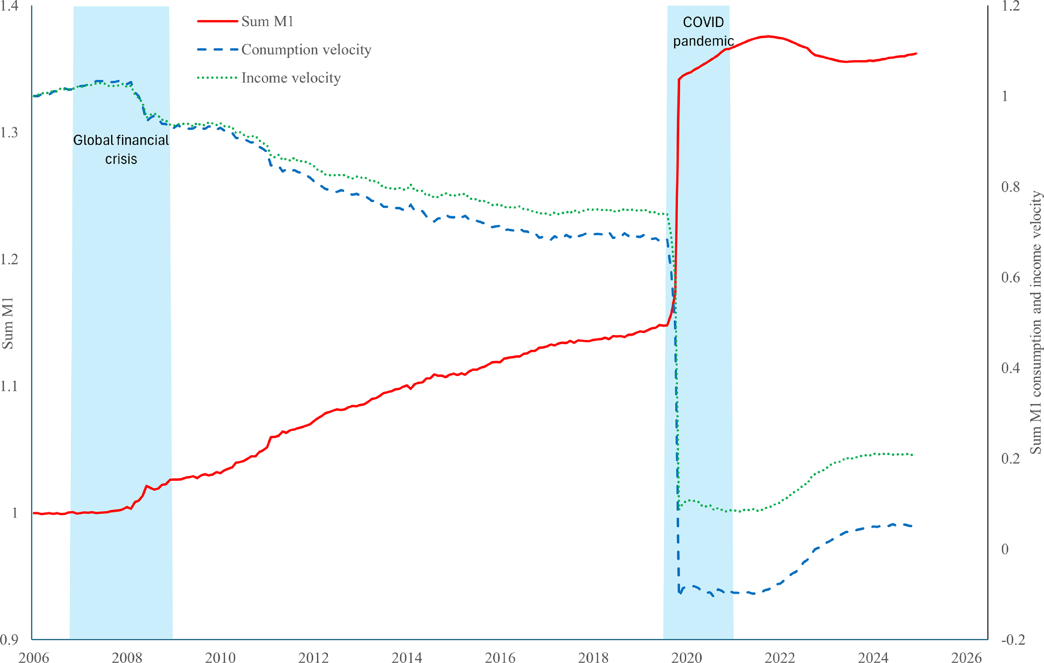
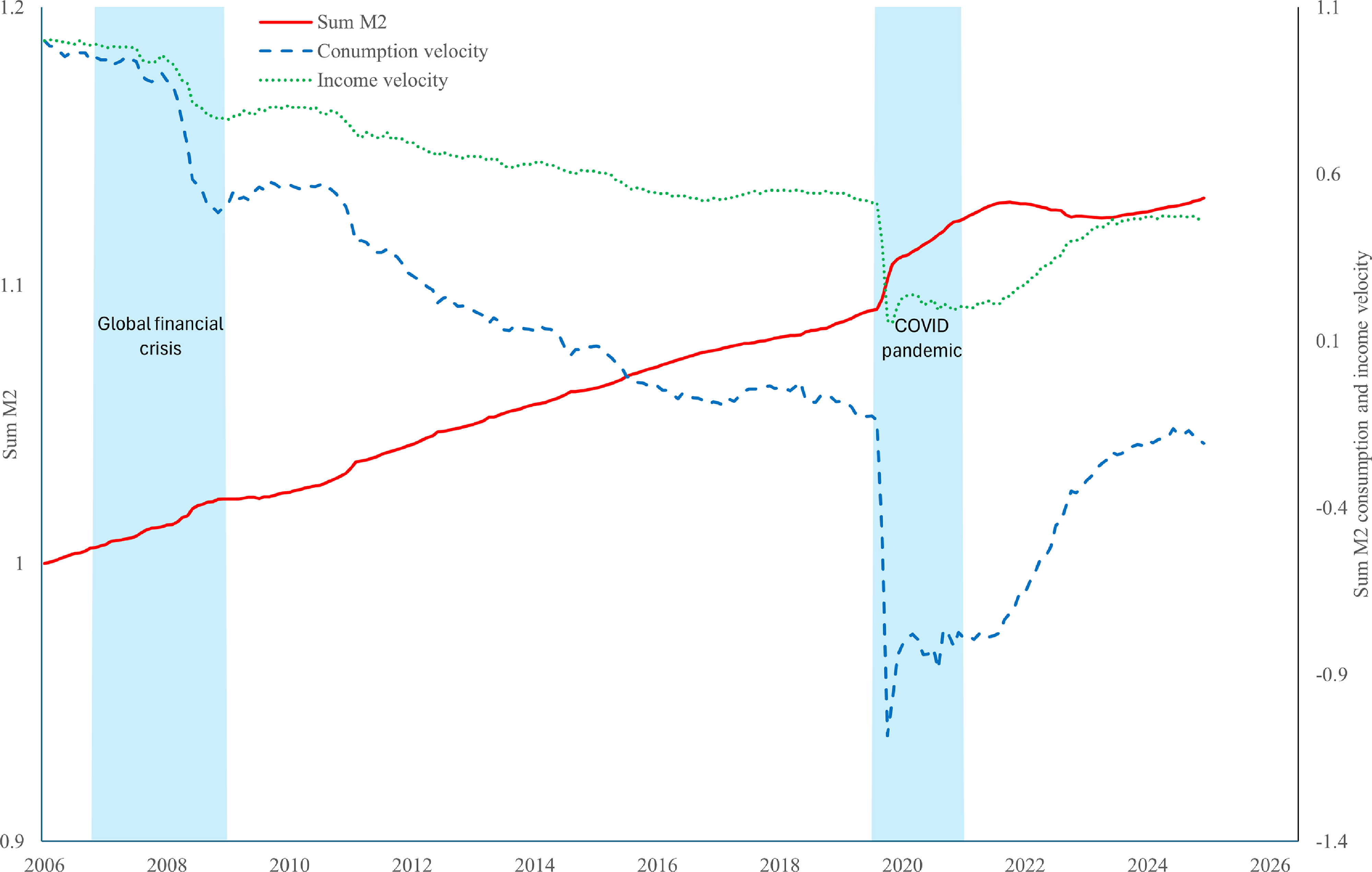
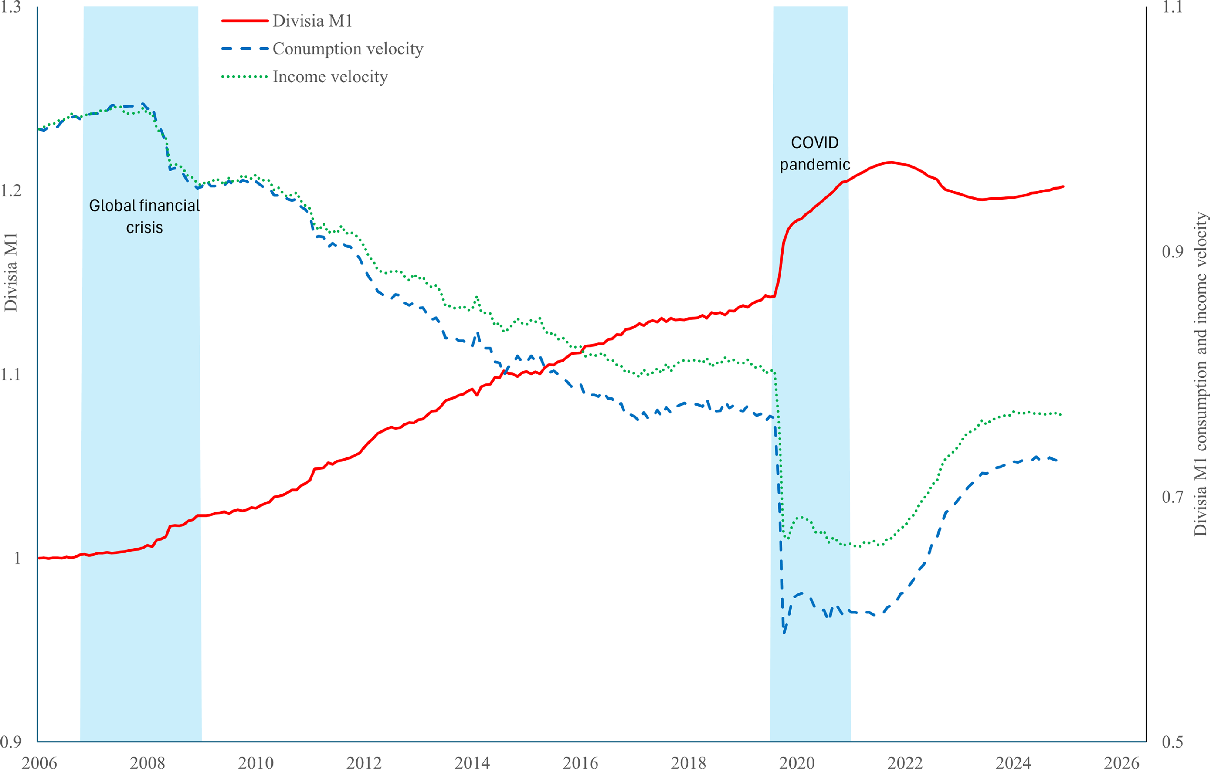
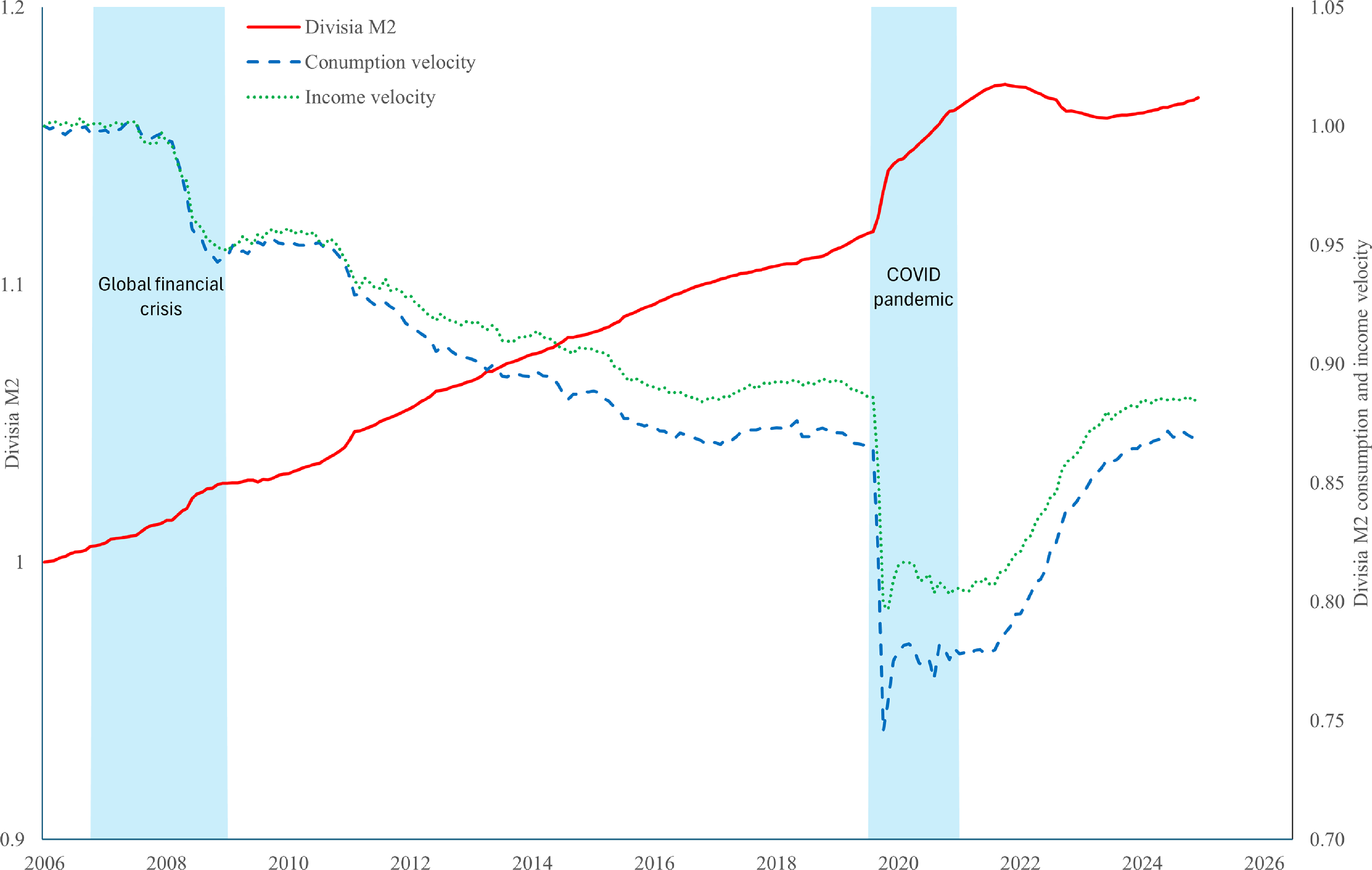
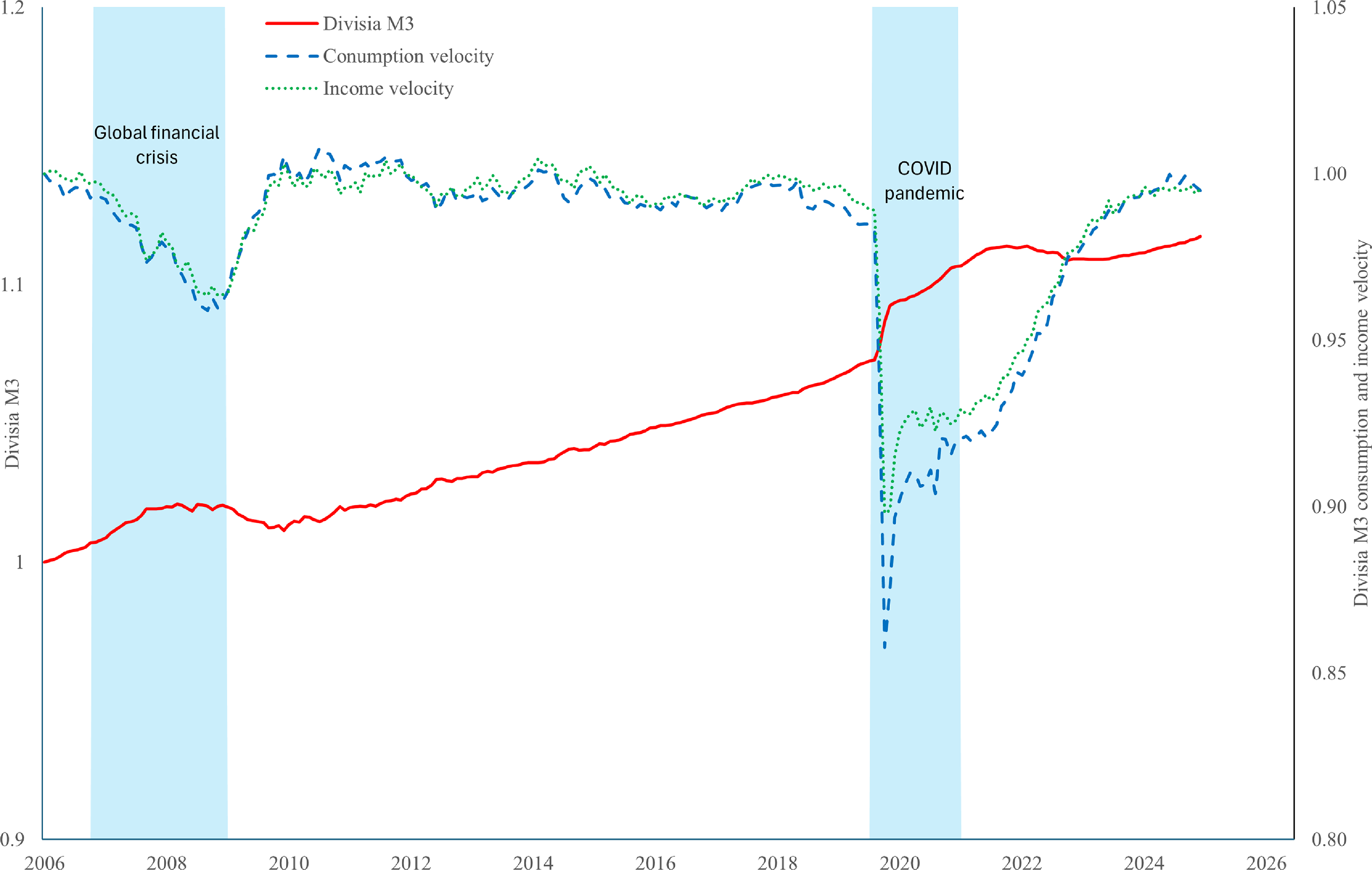
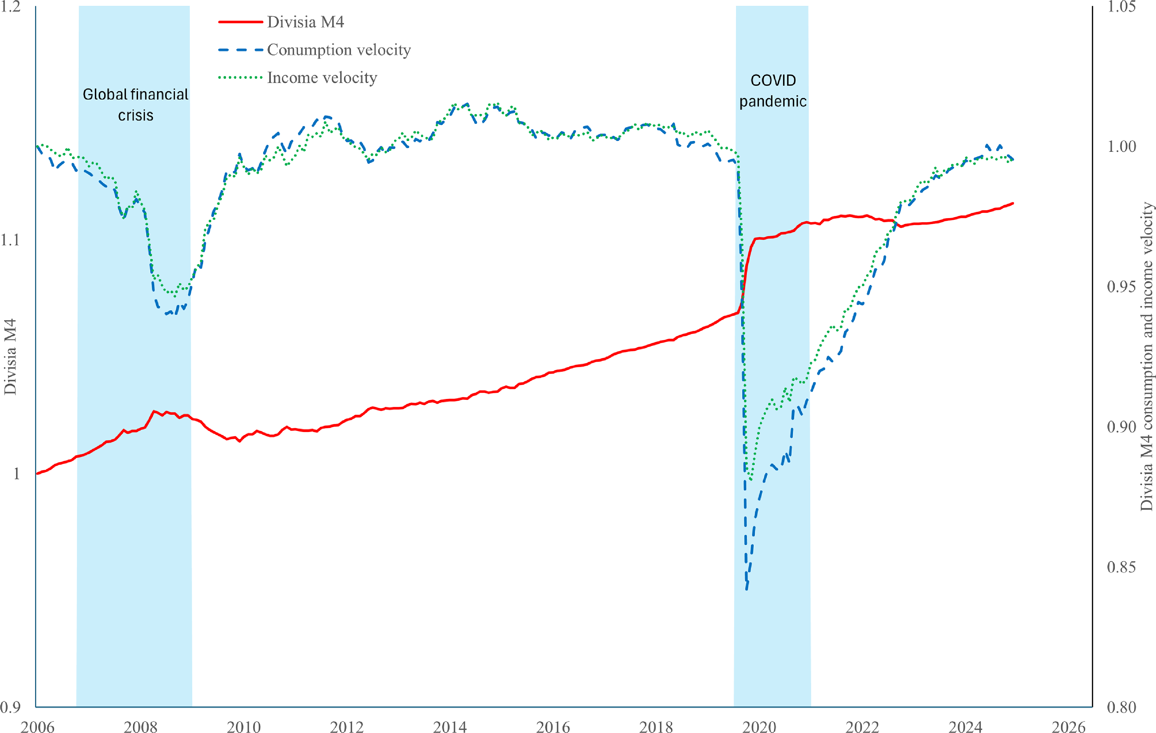
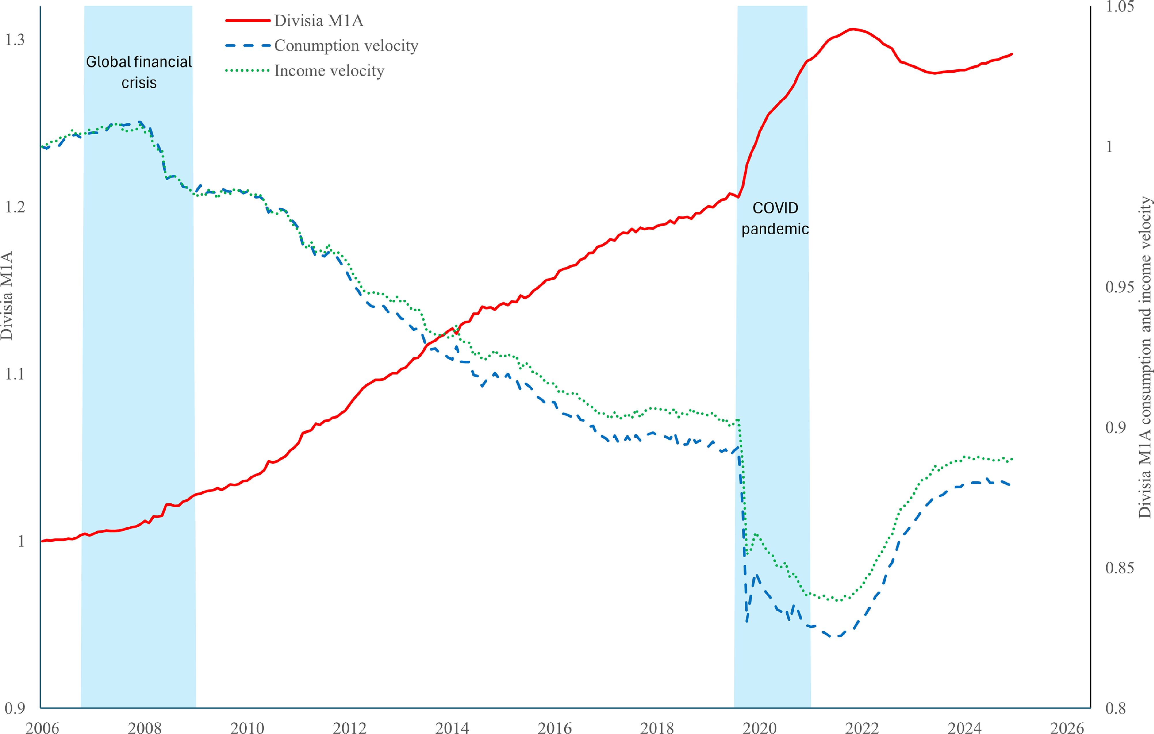
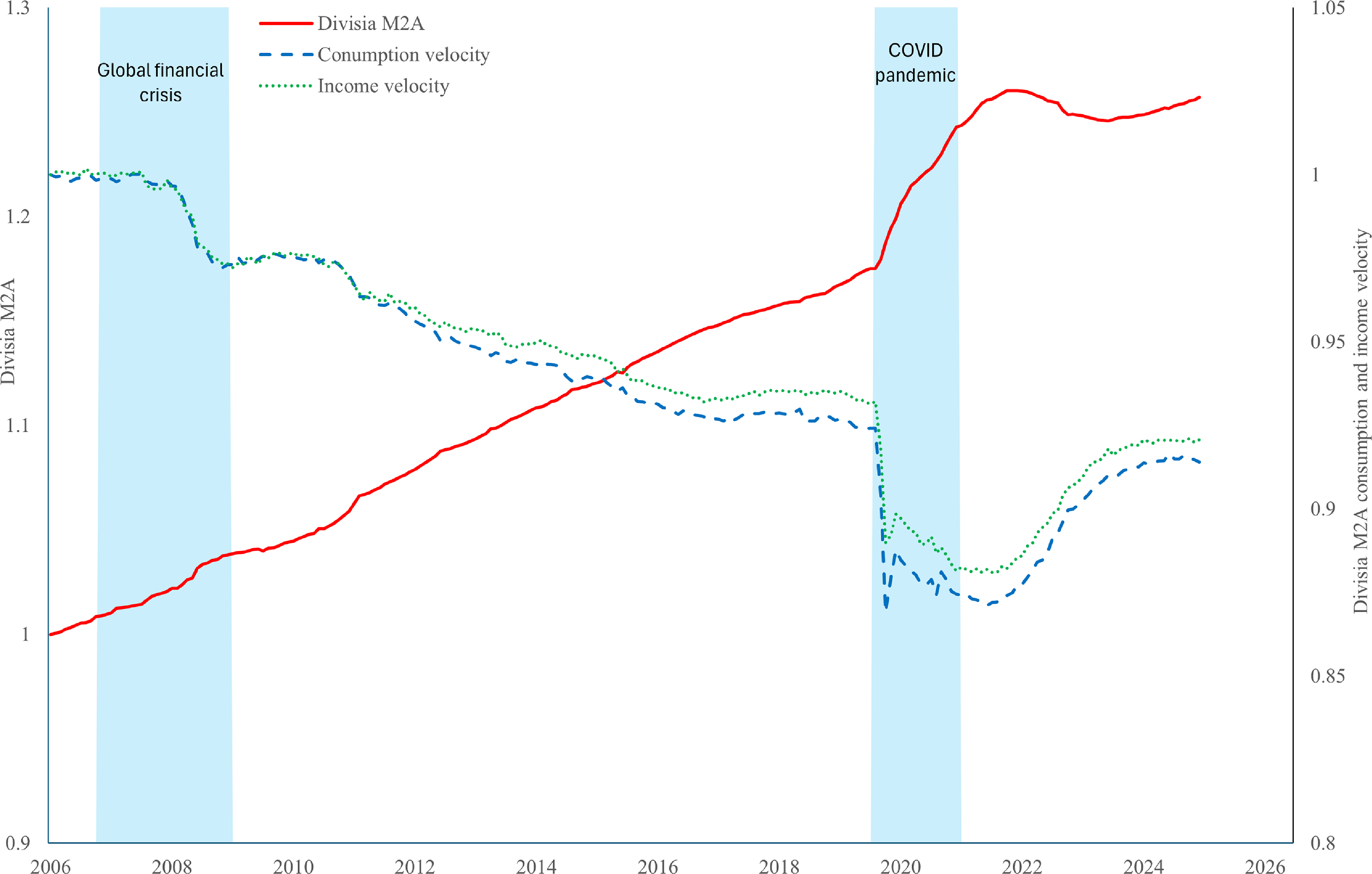
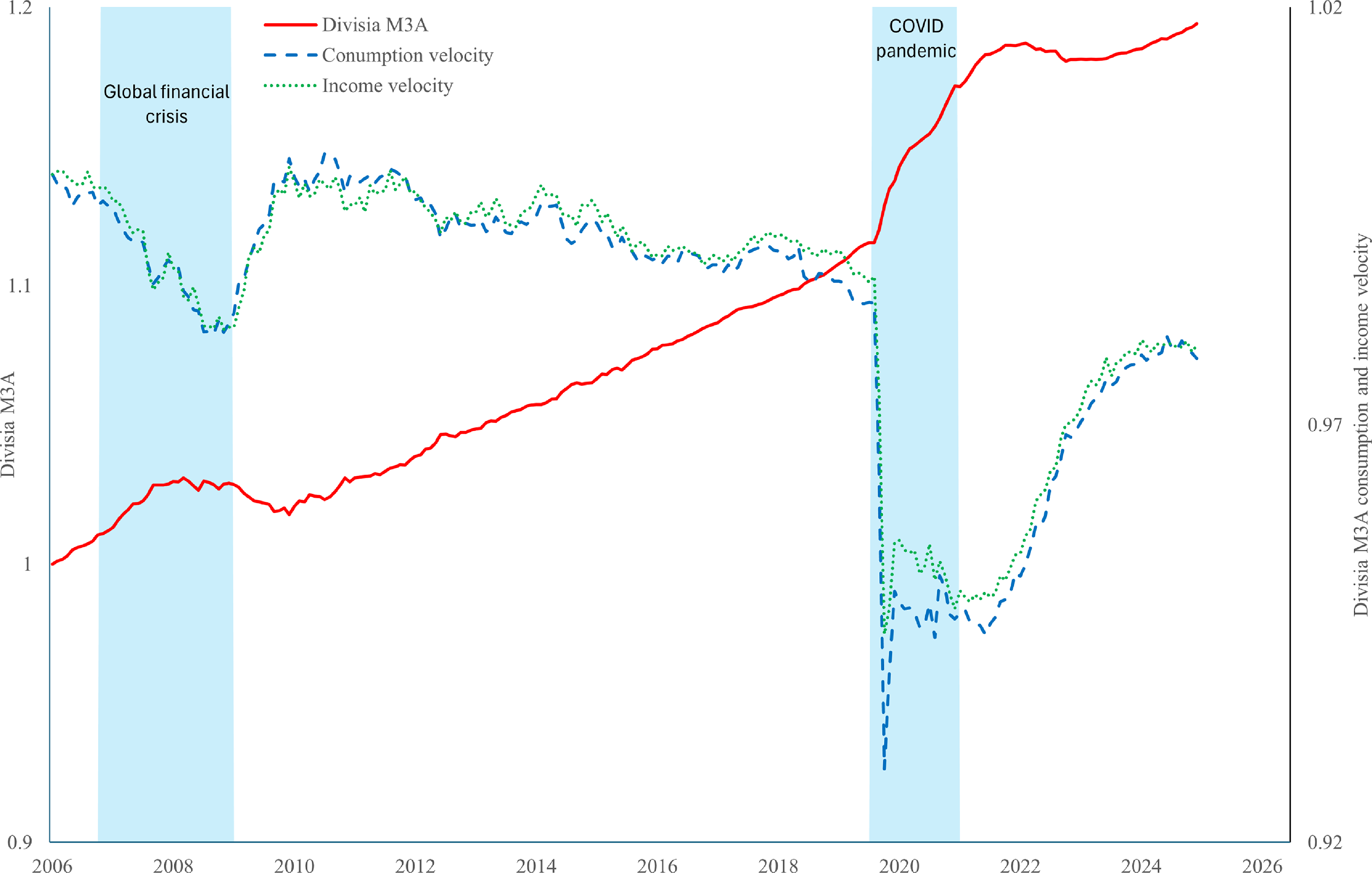
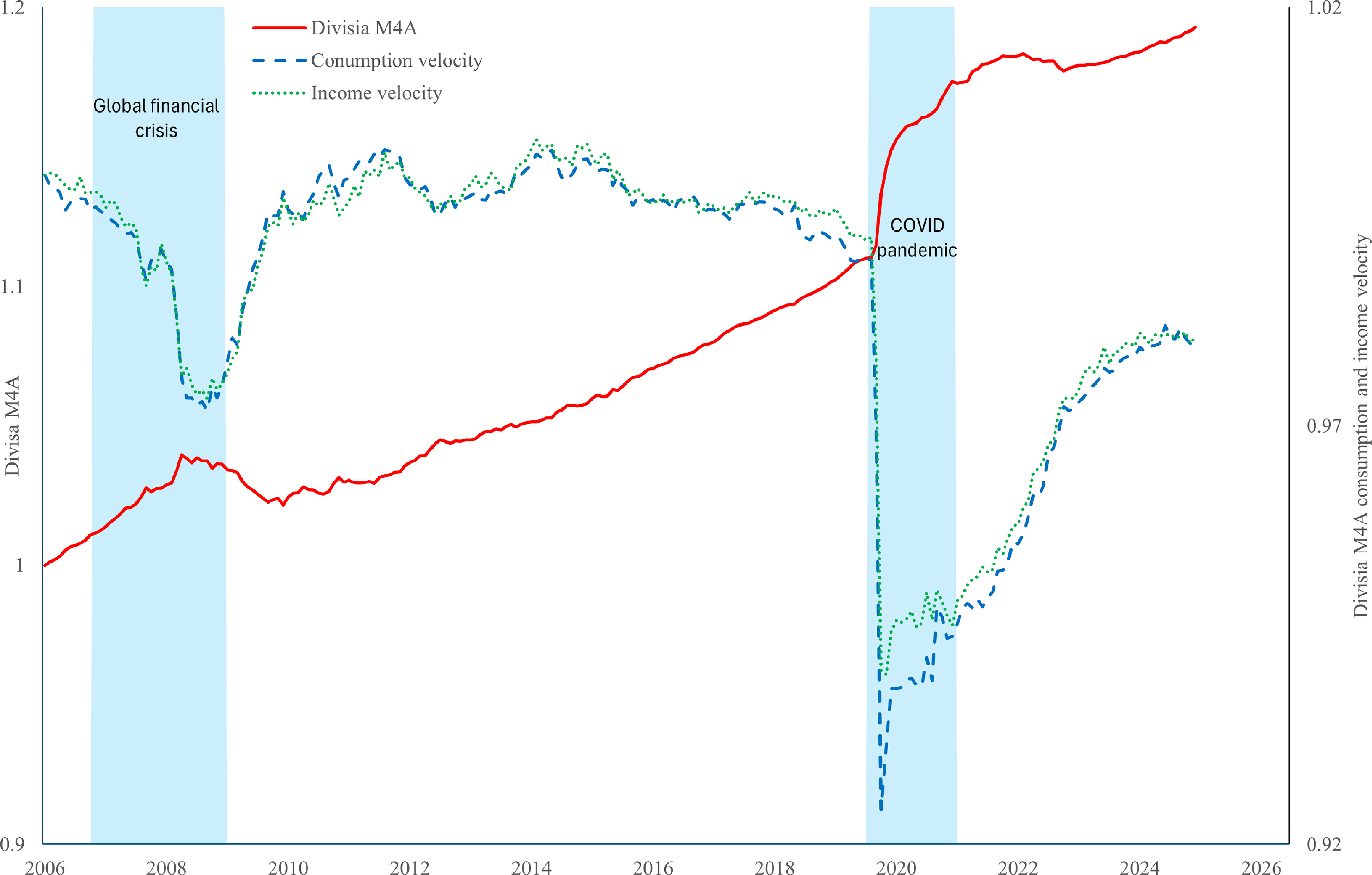
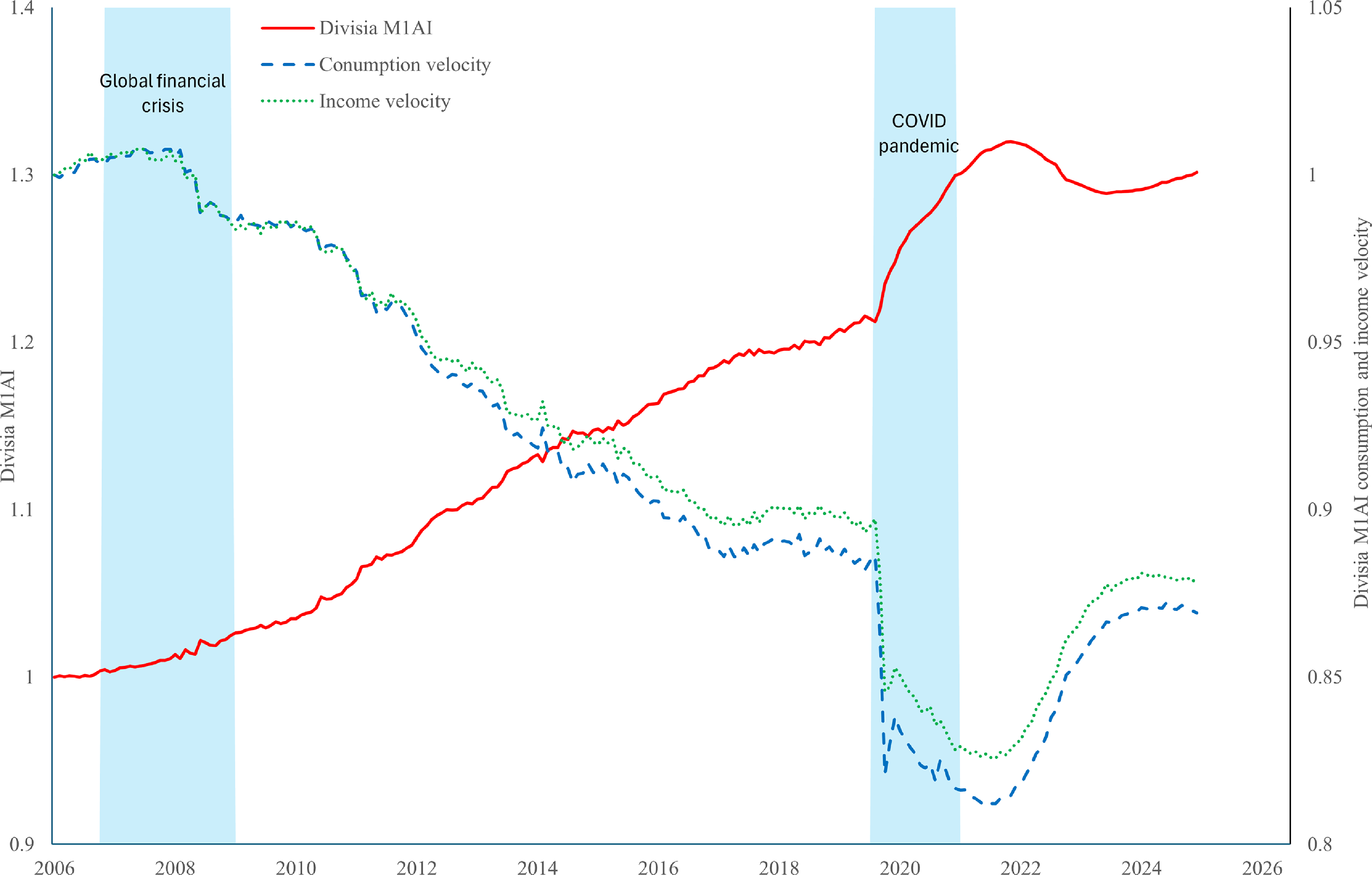
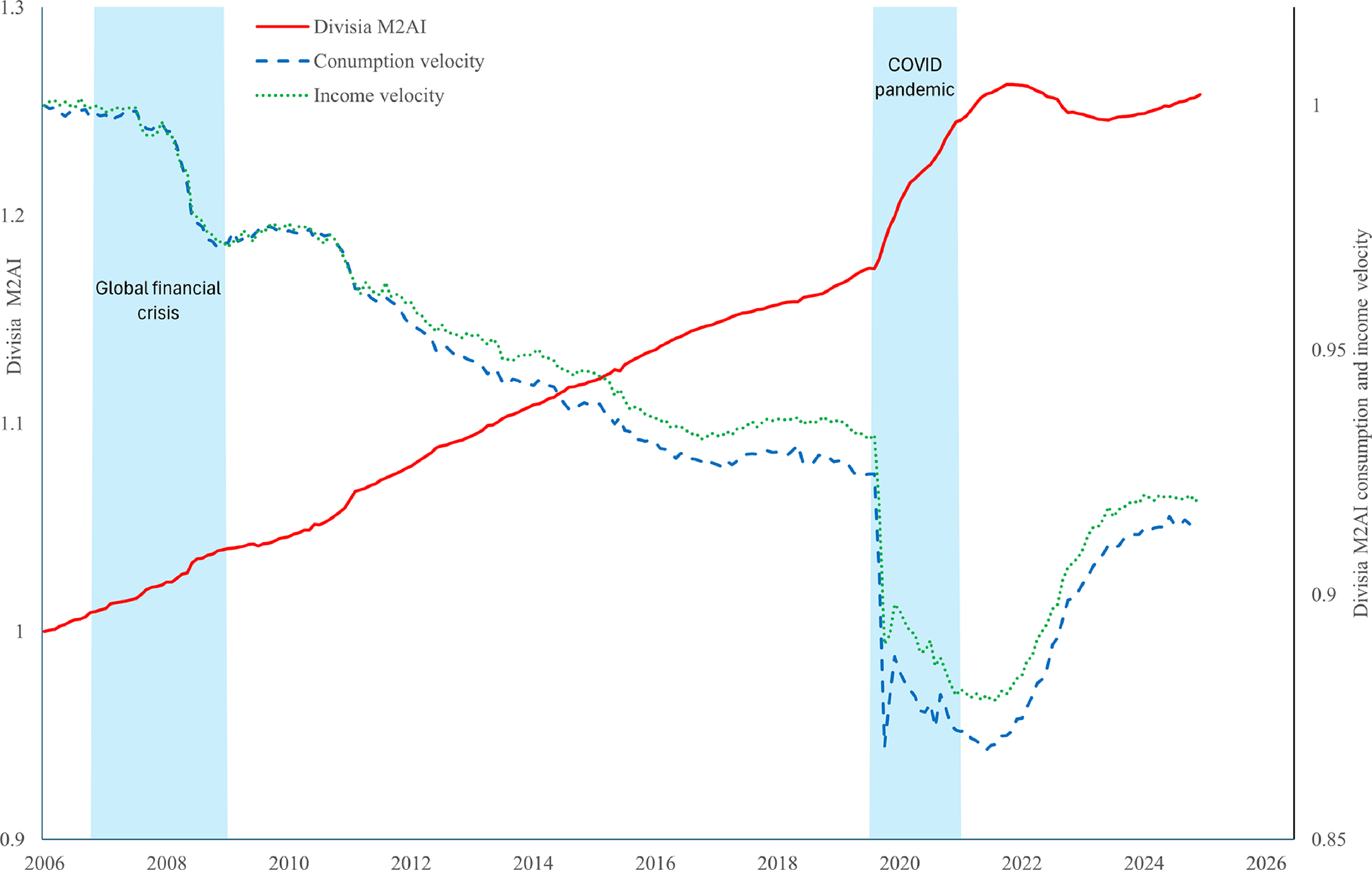
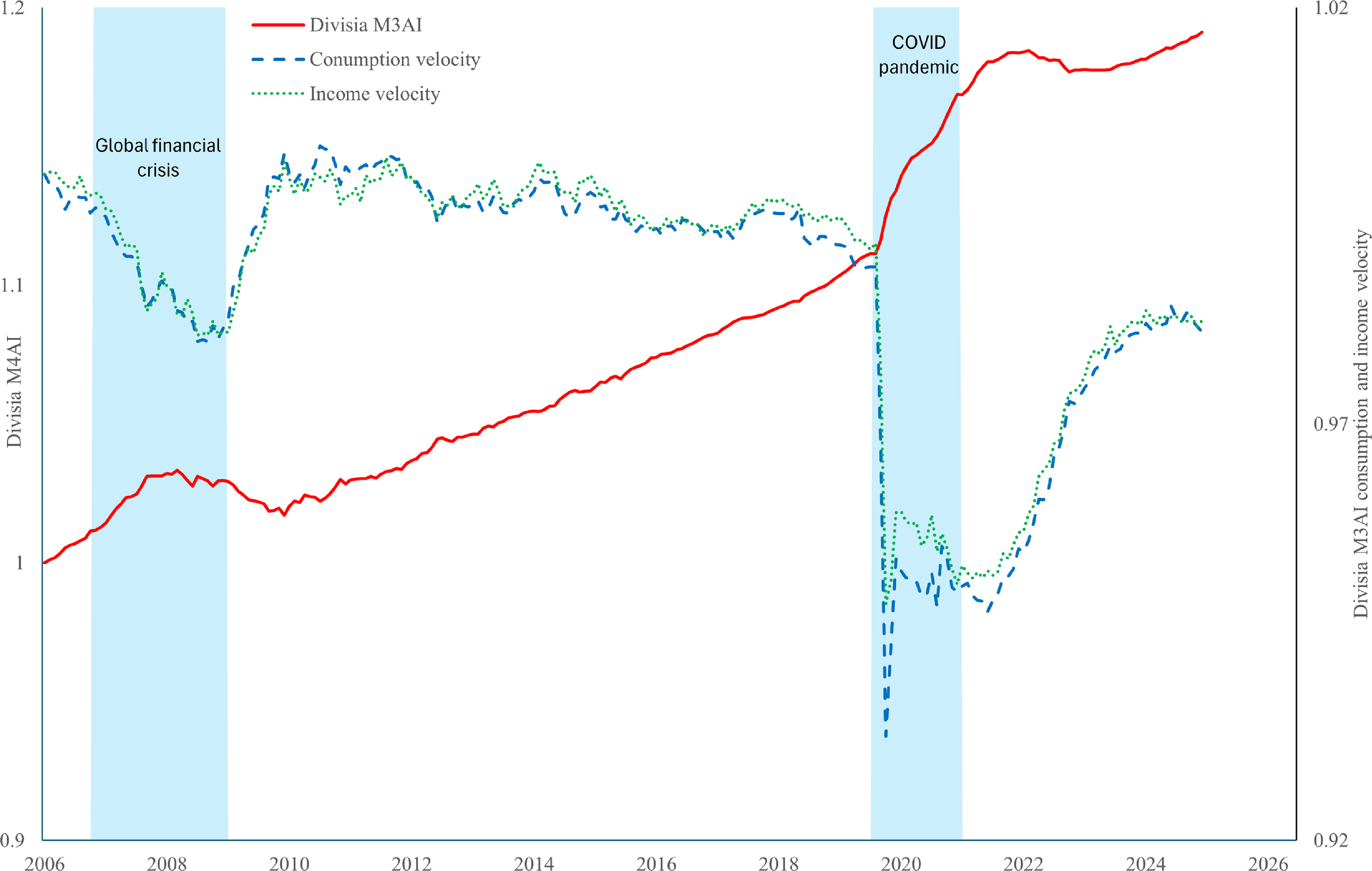
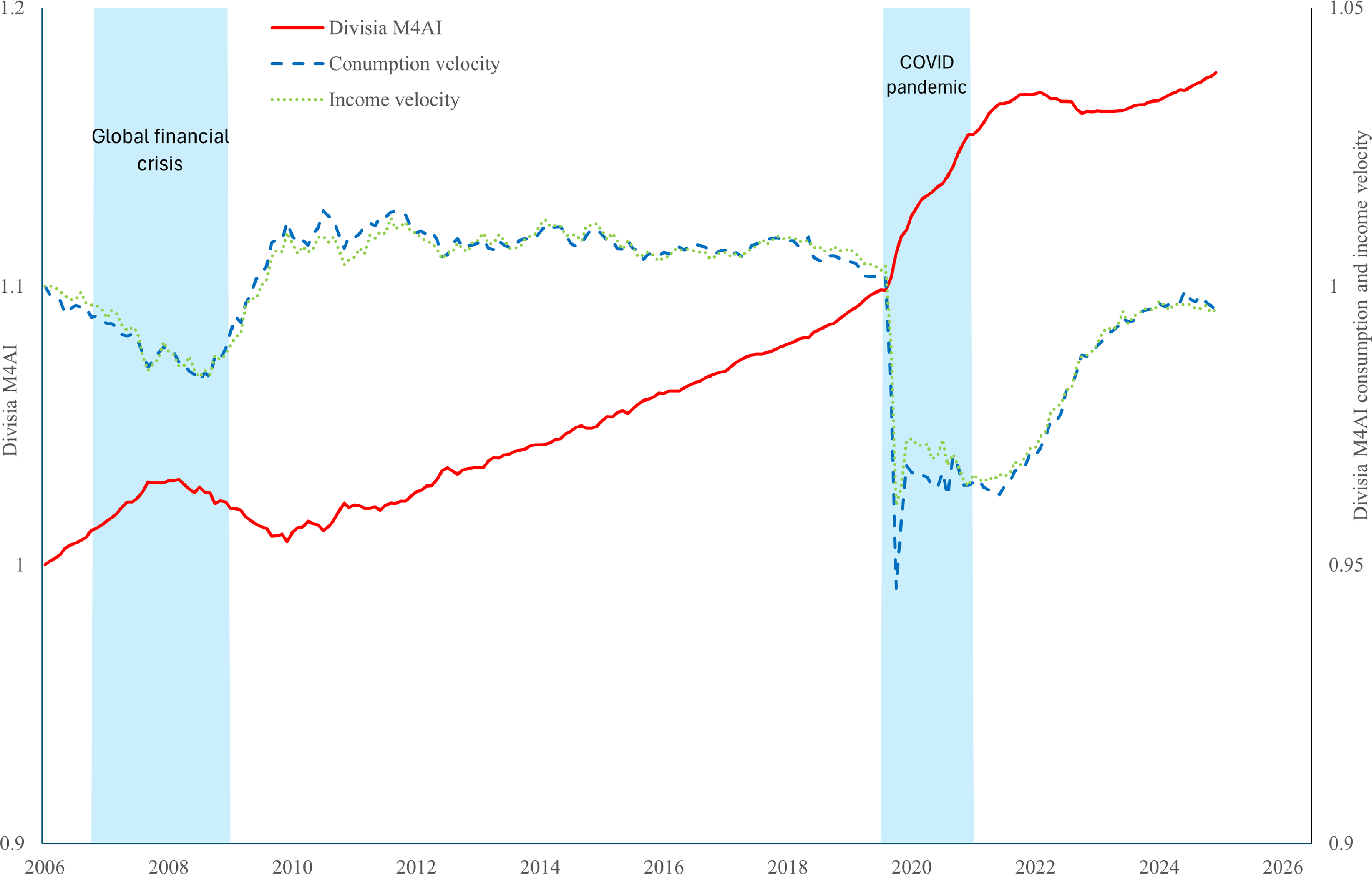
In Figures 1–14, we plot (on the
 $y_{1}$
axis) the logged simple-sum aggregates at the M1 and M2 levels of aggregation and the original Divisia monetary aggregates, the credit card-augmented Divisia aggregates, and the credit card-augmented Divisia inside aggregates at the M1, M2, M3, and M4 levels of aggregation, together with their corresponding consumption and income velocities (on the
 $y_{2}$
axis). To allow easier comparison across the aggregates, each series is normalized to 1 in 2006:m7, and shaded areas indicate the global financial crisis (2007:m6 to 2009:m6) and the Covid-19 recession (2020:m2 to 2021:m6).
The logged Sum Ml aggregate and its consumption and income velocities.
Note: All series are normalized to 1 to 2006:m7.

Figure 1. Long description
A line graph showing the trends of Sum M1, consumption velocity, and income velocity over time. The horizontal axis represents the years from 2006 to 2026, and the vertical axis on the left represents Sum M1 values ranging from 0.9 to 1.4. The vertical axis on the right represents the consumption and income velocity values ranging from 0.2 to 1.2. The graph includes three lines: a solid red line for Sum M1, a dashed blue line for consumption velocity, and a dotted green line for income velocity. Notable events such as the Global financial crisis and the COVID pandemic are highlighted with shaded blue regions. The Sum M1 line shows a steady increase over time, with a significant rise during the COVID pandemic. The consumption velocity and income velocity lines show a general decline over time, with a sharp drop during the COVID pandemic.
The logged Sum M2 aggregate and its consumption and income velocities.
Note: All series are normalized to 1 to 2006:m7.

The logged Divisia Ml aggregate and its consumption and income velocities.
Note: All series are normalized to 1 to 2006:m7.

The logged Divisia M2 aggregate and its consumption and income velocities.
Note: All series are normalized to 1 to 2006:m7.

The logged Divisia M3 aggregate and its consumption and income velocities.
Note: All series are normalized to 1 to 2006:m7.

The logged Divisia M4 aggregate and its consumption and income velocities.
Note: All series are normalized to 1 to 2006:m7.

The logged credit card-augmented Divisia Ml (Divisia MIA) aggregate and its consumption and income velocities.
Note: All series are normalized to 1 to 2006:m7.

The logged credit card-augmented Divisia M2 (Divisia M2A) aggregate and its consumption and income velocities.
Note: All series are normalized to 1 to 2006:m7.

The logged credit card-augmented Divisia M3 (Divisia M3A) aggregate and its consumption and income velocities.
Note: All series are normalized to 1 in 2006:m7.

The logged credit card-augmented Divisia M4 (Divisia M4A) aggregate and its consumption and income velocities.
Note: All series are normalized to 1 in 2006:m7.

The logged credit card-augmented Divisia inside Ml (Divisia MlAI) aggregate and its consumption and income velocities.
Note: All series are normalized to 1 in 2006:m7.

The logged credit card-augmented Divisia inside M2 (Divisia M2AI) aggregate and its consumption and income velocities.
Note: All series are normalized to 1 in 2006:m7.

The logged credit card-augmented Divisia inside M3 (Divisia M3AI) aggregate and its consumption and income velocities.
Note: All series are normalized to 1 in 2006:m7.

The logged credit card-augmented Divisia inside M4 (Divisia M4AI) aggregate and its consumption and income velocities.
Note: All series are normalized to 1 in 2006:m7.

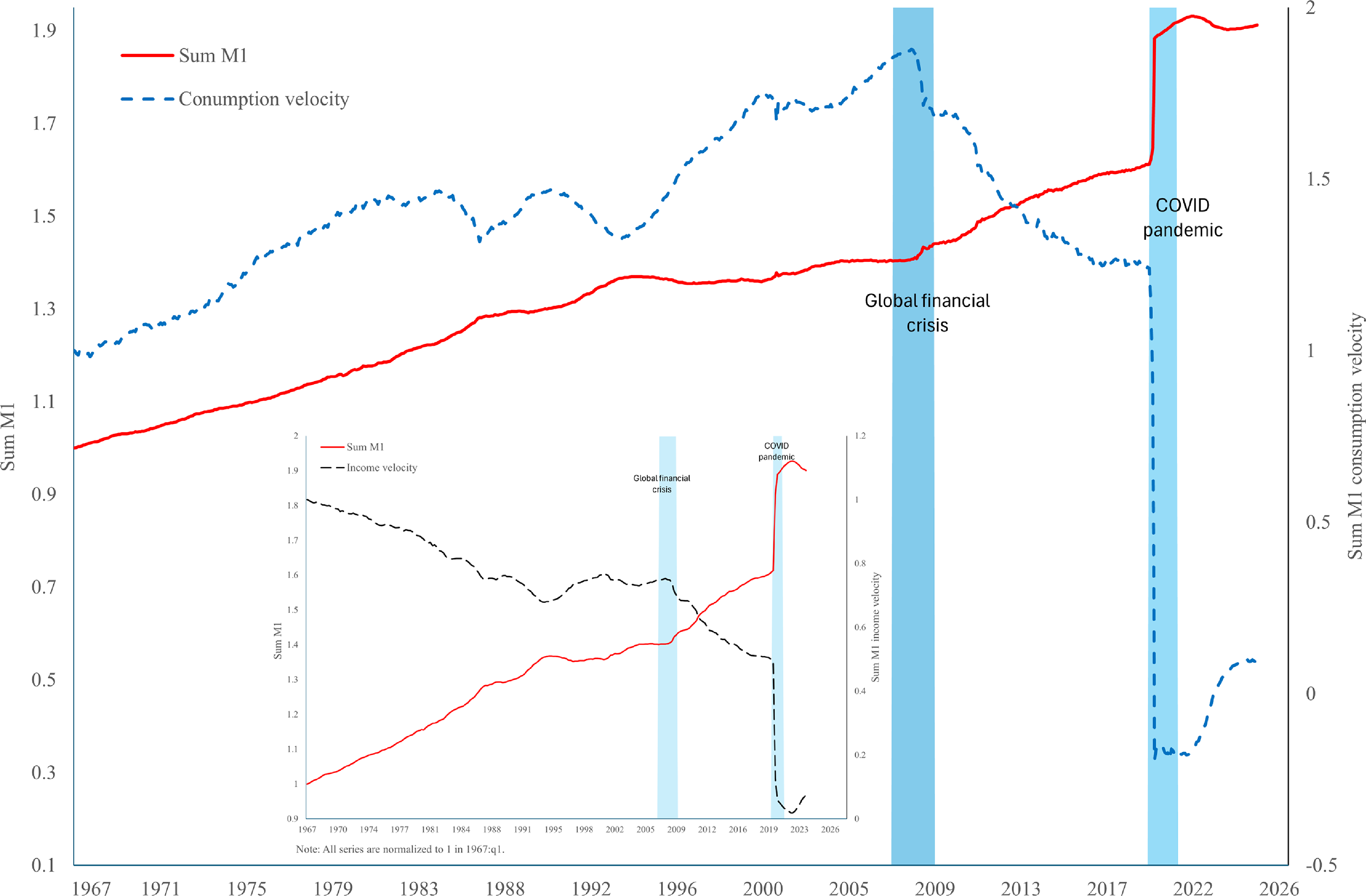
As can be seen in Figures 1 and 2, the simple-sum aggregates show steady growth until early 2020, with a modest rise during the financial crisis, followed by a sharp increase during Covid pandemic. Both consumption and income velocities of Sum M1 fall steadily, with a sharp drop during Covid and a mild recovery in recent years. Sum M2 shows a similar pattern in Figure 2, though with a milder drop during Covid compared to Sum M1. Figures 3–6 plot the original Divisia aggregates and their consumption and income velocities. Divisia M1 and Divisia M2 rise over time while their velocities fall, with clear responses during the global financial crisis and the Covid-19 recession. These responses are easier to see than those for the simple-sum aggregates. Regarding Divisia M3 and Divisia M4, the aggregates grow over time, but their velocities remain comparatively more stable in non-crisis periods. However, their velocities respond during crises in a way similar to the narrower Divisia measures and more strongly than the simple-sum aggregates, especially during the global financial crisis.
Figures 7–10 plot the credit card-augmented Divisia monetary aggregates and their corresponding velocities. The relationship between the aggregates and velocities resembles that observed for the original Divisia measures. In particular, we observe a negative relationship between the dynamics of the monetary aggregates and velocities during the two crisis periods across all four aggregation levels, with stronger effects for broader measures such as Divisia M3A and Divisia M4A. Outside crisis periods, the relationship appears more pronounced for narrower measures of the credit card-augmented Divisia aggregates than for broader measures. Finally, Figures 11–14 show the credit card-augmented Divisia inside monetary aggregates and their associated velocities. The interaction between the aggregates and velocities closely mirrors that observed for the original Divisia and the credit card-augmented Divisia measures. The credit card-augmented Divisia inside aggregates and their velocities move in opposite directions during crisis periods, with stronger effects for broader measures. We also observe that velocities respond less to changes in the aggregates during non-crisis periods for broader Divisia inside measures compared with narrower aggregation levels, consistent with the patterns seen for the credit card-augmented Divisia measures.
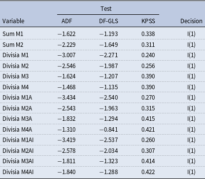
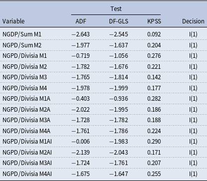
Unit root and stationarity tests for the monetary aggregates

Table 1. Long description
A table with 14 rows and 5 columns. The columns are labeled Test, Variable, ADF, DF-GLS, KPSS, and Decision. The table presents the results of unit root and stationarity tests for various monetary aggregates. Each row lists a different variable, followed by the corresponding test results and a decision indicating whether a unit root in levels was found. The variables include Sum M1, Sum M2, Divisia M1, Divisia M2, Divisia M3, Divisia M4, Divisia M1A, Divisia M2A, Divisia M3A, Divisia M4A, Divisia M1AI, Divisia M2AI, Divisia M3AI, and Divisia M4AI. The test results are numerical values, and the decision column consistently shows I(1) for all variables, indicating a unit root in levels found by at least two of the tests.
Notes: The sample period is 2006:m7 to 2025:m6.
The 5 percent critical values for the ADF, DF-GLS, and KPSS tests are −3.430, −2.925, and 0.146, respectively.
Decision of I(1) indicates unit root in levels found by at least two of the tests.
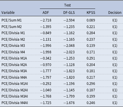
We also investigate the unit root properties of the variables, since our econometric methodology in the next section requires all variables included in the models to be stationary. In this regard, Tables 1–3 summarize the results of unit root tests for the logged monetary aggregates and their consumption and income velocities. All three tables report tests of the null hypothesis of a unit root against the alternative of stationarity, using the Augmented Dickey-Fuller (ADF) test [see Dickey and Fuller (Reference Dickey and Fuller1981)] and the Dickey-Fuller GLS (DF-GLS) test [see Elliott et al. (Reference Elliott, Rothenberg and Stock1996)], allowing for both a constant and a trend in the specifications. In both tests we use the Akaike Information Criterion to select the optimal lag length. In addition, because of the low power of the ADF and DF-GLS tests against trend-stationary alternatives, we also report results from the KPSS test [see Kwiatkowski et al. (Reference Kwiatkowski, Phillips, Schmidt and Shin1992)] which tests the null hypothesis of stationarity around a constant and trend against the alternative of a unit root. All three tests indicate that the monetary aggregates and their consumption and income velocities are stationary in first differences, that is, integrated of order one [or I(1) in the terminology of Engle and Granger (Reference Engle and Granger1987)]. As a result, in the econometric work that follows we use the growth rates of the series.
Unit root and stationarity tests for the consumption velocities

Table 2. Long description
A table with 12 rows and 5 columns. The columns are labeled Variable, ADF, DF-GLS, KPSS, and Decision. The table presents the results of unit root tests for various monetary aggregates and their consumption velocities. Each row lists a different variable, followed by the test results for ADF, DF-GLS, and KPSS, and the decision indicating whether the variable is integrated of order one (I(1)). Row 1: PCE/Sum M1, 2.718, 2.594, 0.089, I(1). Row 2: PCE/Sum M2, 1.395, 1.235, 0.221, I(1). Row 3: PCE/Divisia M1, 0.849, 1.162, 0.284, I(1). Row 4: PCE/Divisia M2, 1.131, 1.165, 0.237, I(1). Row 5: PCE/Divisia M3, 1.996, 2.048, 0.139, I(1). Row 6: PCE/Divisia M4, 1.998, 2.023, 0.171, I(1). Row 7: PCE/Divisia M1A, 0.342, 1.253, 0.291, I(1). Row 8: PCE/Divisia M2A, 0.970, 1.128, 0.204, I(1). Row 9: PCE/Divisia M3A, 1.777, 1.823, 0.181, I(1). Row 10: PCE/Divisia M4A, 1.797, 1.820, 0.217, I(1). Row 11: PCE/Divisia M1AI, 0.292, 1.196, 0.296, I(1). Row 12: PCE/Divisia M2AI, 1.040, 1.145, 0.187, I(1). Row 13: PCE/Divisia M3AI, 1.768, 1.799, 0.199, I(1). Row 14: PCE/Divisia M4AI, 1.725, 1.676, 0.246, I(1).
Note: See notes to Table 1.
Unit root and stationarity tests for the income velocities

Table 3 Long description
A table summarizing unit root and stationarity tests for income velocities. The table has 14 rows and 5 columns. The columns are labeled Test, Variable, ADF, DF-GLS, KPSS, and Decision. The rows list different variables and their corresponding test results. Row 1: NGDP/Sum M1, 2.643, 2.545, 0.092, I(1). Row 2: NGDP/Sum M2, 1.977, 1.637, 0.204, I(1). Row 3: NGPD/Divisia M1, 0.719, 1.056, 0.276, I(1). Row 4: NGPD/Divisia M2, 1.782, 1.676, 0.221, I(1). Row 5: NGPD/Divisia M3, 1.765, 1.814, 0.142, I(1). Row 6: NGPD/Divisia M4, 1.978, 1.999, 0.177, I(1). Row 7: NGPD/Divisia M1A, 0.403, 0.936, 0.282, I(1). Row 8: NGPD/Divisia M2A, 2.022, 1.995, 0.186, I(1). Row 9: NGPD/Divisia M3A, 1.728, 1.782, 0.188, I(1). Row 10: NGPD/Divisia M4A, 1.761, 1.786, 0.224, I(1). Row 11: NGPD/Divisia M1AI, 0.006, 1.983, 0.290, I(1). Row 12: NGPD/Divisia M2AI, 2.139, 2.043, 0.171, I(1). Row 13: NGPD/Divisia M3AI, 1.724, 1.761, 0.207, I(1). Row 14: NGPD/Divisia M4AI, 1.675, 1.647, 0.255, I(1).
Note: See notes to Table 1.
4. Empirical results
4.1 Granger causality tests
Hall and Noble (Reference Hall and Noble1987), Brocato and Smith (Reference Brocato and Smith1989), Mehra (Reference Mehra1989), Fisher and Serletis (Reference Fisher and Serletis1989), and Thornton (Reference Thornton1995) all use the Granger-causality method to test Friedman’s hypothesis that money growth volatility is causal factor in changes in velocity. In doing so, they assume that the relevant information is contained in the present and past values of these variables and use the following bivariate autoregressive representation
 \begin{equation} v_{t}=\alpha _{0}+\sum _{j=1}^{r}\mathbf{\alpha }_{j}v_{t-j}+\sum _{j=1}^{s} \mathbf{\beta }_{j}\text{VOL}_{t-j}+\varepsilon _{t} \end{equation}
where
 $\Delta$
is the difference operator,
 $v_{t}=\Delta \log V_{t}$
,
 $ V_{t}$
is the level of money velocity, VOL
 $_{t}$
is the level of money growth volatility, and
 $\varepsilon _{t}$
is a white noise disturbance. Here, VOL
 $_{t}$
is a 12-month moving standard deviation of money growth. Given the monthly frequency of the data, the 12-month window captures annual cyclical variation while smoothing short-term fluctuations, a choice commonly adopted in the literature to balance responsiveness and stability in volatility measurement.
In this framework, the Granger procedure requires that we first estimate equation (4) by ordinary least squares to obtain the unrestricted sum of squared residuals,
 $SSR_{u}$
. Then, by running another regression under the restriction that all
 $\beta _{j}$
’s are zero, the restricted sum of squared residuals,
 $SSR_{r}$
, is obtained. If
 $\varepsilon _{t}$
is white noise, then the statistic
 \begin{equation*} \frac {\left ( SSR_{r}-SSR_{u}\right ) /s}{SSR_{u}/\left ( T-r-s-1\right ) } \end{equation*}
has an asymptotic
 $F$
-distribution with the numerator having degrees of freedom of
 $s$
and the denominator of
 $T-r-s-1$
where
 $T$
is the number of observations and 1 is subtracted out to account for the constant term in equation (4). If the null hypothesis of
 $\widehat {\beta } _{j}=0$
for
 $j=1,\cdot \cdot \cdot ,s$
cannot be rejected, then the conclusion is that the data do not show causality. If the null hypothesis is rejected, then the conclusion is that the data do show causality.
For monetary variability, the literature has produced mixed results. In particular, Hall and Noble (Reference Hall and Noble1987) using quarterly data (from 1963:1 to 1984:2), define monetary variability as an eight-quarter standard deviation of M1 growth, and find a causal relation from money growth variability to velocity. Fisher and Serletis (Reference Fisher and Serletis1989) test the same hypothesis that Hall and Noble (Reference Hall and Noble1987) did, using monthly U.S. data (covering the period 1970 through mid-1985), and search for the relationship over nine simple-sum and Divisia measures of the money stock, in an attempt to deal with anomalies that arise because of different definitions of money. Although they find some slight differences across the different monetary aggregates of equal breadth, they claim that the influence of money growth variability shows up on velocity in a (Granger-) causal sense.
However, Brocato and Smith (Reference Brocato and Smith1989), using monthly U.S. data from 1962:2 through 1985:9, reestimate the Hall and Noble (Reference Hall and Noble1987) equation over the full period, as well as over pre- and post-October 1979 periods. They find evidence to support the Friedman hypothesis in the pre-October 1979 period but find no evidence that the variability of money growth influenced velocity thereafter. They conclude that the change in Federal Reserve operating procedures in October 1979 contributed to a break down in the money growth/velocity growth relationship and that this finding runs counter to the Friedman hypothesis which would suggest stronger causality results after 1979, given the increase in money growth variability that took place. The Brocato and Smith (Reference Brocato and Smith1989) finding has also been confirmed by Mehra (Reference Mehra1989) who shows that the Granger-causality result reported by Hall and Noble (Reference Hall and Noble1987) is not robust to some changes of specification and the sample period. Moreover, Thornton (Reference Thornton1995) extends this work by testing Friedman’s hypothesis using quarterly data (over the period from 1961 to 1990) for nine countries—Australia, Austria, Canada, France, Germany, Italy, Japan, Switzerland, and the United Kingdom. He finds no evidence of the hypothesis that money supply volatility causes income velocity to change and concludes that “the Friedman hypothesis would appear to have little general applicability.”
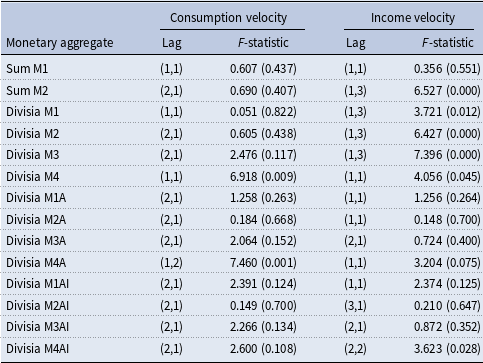
We report our results, using monthly data over the 2006:m7 to 2025:m6 period, in the second and third columns of Table 4. For each monetary aggregate, we select the model using the SIC to obtain a parsimonious lag structure. As shown in the second column of Table 4, the selected lag structure for Sum M1 and Sum M2 is (1,1) and (1,2), respectively. For the original Divisia aggregates, the lag structure is (1,1) for Divisia M1 and Divisia M4 and (2,1) for Divisia M2 and Divisia M3. For all the credit card-augmented Divisia aggregates and credit card-augmented Divisia inside monetary aggregates the chosen lag structure is (2,1), except for Divisia M4A for which the SIC suggests a lag structure of (1,2). After estimating each model with its selected lag structure, we conduct the Granger-causality tests based on equation (4). The
 $p$
-values indicate that monetary variability affects the consumption velocity of money only with the Divisia M4 and Divisia M4A aggregates with
 $p$
-values of
 $0.009$
and
 $0.001$
, respectively. Thus, only two of the fourteen monetary aggregates show a statistically significant link between the variability of money growth and the consumption velocity.
Granger causality tests from the variability of money growth to the velocity of money

Table 4 Long description
A table titled ’Granger causality tests from the variability of money growth to the velocity of money’ presents data on the relationship between monetary aggregates and their consumption and income velocities. The table has 14 rows and 6 columns, including headers. The columns are labeled ’Monetary aggregate’, ’Consumption velocity Lag’, ’Consumption velocity F-statistic’, ’Income velocity Lag’, and ’Income velocity F-statistic’. Each row corresponds to a different monetary aggregate, such as Sum M1, Sum M2, Divisia M1, etc. The table reports lag structures and F-statistic values with corresponding p-values in parentheses. For example, Sum M1 has a lag structure of (1,1) for both consumption and income velocity, with F-statistic values of 0.607 and 0.356, respectively. Divisia M4 shows significant results with an F-statistic of 6.918 for consumption velocity and 4.056 for income velocity. The table notes that the sample period is from 2006:m7 to 2025:m6, and lag structures are selected based on the minimum SIC value by evaluating 144 regressions.
Notes: The sample period is 2006:m7 to 2025:m6.
Lag structures are selected based on the minimum SIC value by evaluating 144 regressions.
Numbers in parentheses are p-values.
Next, we compare the above findings with the results reported in the third and fourth columns of Table 4 which use the income velocity of money. In most cases, the selected lag structures differ from those based on the consumption velocity. For the simple-sum aggregates, the chosen lag structure is (1,1) for Sum M1 and (1,3) for Sum M2. For the original Divisia aggregates, the optimal lag structure is (1,3) for Divisia M1, Divisia M2, and Divisia M4, while the model for Divisia M3 is (1,1). In the case of the credit card-augmented Divisia aggregates, the optimal lag structure is (1,1) for Divisia M1A, Divisia M2A, and Divisia M4A, which differ from their corresponding lag structures based on the consumption velocity. The lag structure for Divisia M3A is (2,1), which coincides with the specification based on the consumption velocity. For the credit card-augmented Divisia inside aggregates, the selected lag structure is (1,1) for M1AI, (3,1) for M2AI, (2,1) for M3AI, and (2,2) for M4AI, again differing from most specifications based on the consumption velocity, except for the Divisia M3AI aggregate. The Granger-causality test
 $p$
-values in fifth column of Table 4 show that monetary variability based on Sum M2, all four original Divisia aggregates, and Divisia M4A Granger causes the income velocity at the 5 percent level of significance. Hence, six of the fourteen monetary aggregates exhibit a statistically significant relationship between money growth variability and the income velocity.
Overall, we conclude that the Granger-causality results provide weak support for Friedman’s hypothesis across most monetary aggregates. This pattern suggests that the velocity of money remains largely stable in the presence of money growth volatility.
4.2 A structural GARCH-in-mean VAR model
The Granger causality approach relies on ad hoc non-parametric moving standard deviation to measure monetary variability. In this section we use a structural model, based on Elder and Serletis (Reference Elder and Serletis2010). In the model, a vector autoregression (VAR) captures the joint dynamics of the variables by allowing each variable to depend on its own past values as well as the past values of the other variables in the system. This approach addresses the dynamic interactions between money growth and the velocity of money. To account for time-varying uncertainty, we augment the VAR with a generalized autoregressive conditional heteroskedasticity (GARCH) structure, which models monetary uncertainty as the conditional standard deviation of the one-step-ahead forecast error given the contemporaneous information set.
This combined framework allows us to jointly analyze the evolution of monetary dynamics and the role of uncertainty. Here, the model is a bivariate structural VAR in the monetary growth rate and the growth rate of the velocity of money, as follows
 \begin{align} \boldsymbol{B}\boldsymbol{z}_{t}=\boldsymbol{C}+\sum _{j=1}^{p}\mathbf{\Gamma }_{j} \boldsymbol{z}_{t-j}+\boldsymbol{\Lambda } \boldsymbol{H}_{t}^{1/2}+\boldsymbol{\epsilon }_{t} \\[-35pt] \nonumber \end{align}
 \begin{align*} \boldsymbol{\epsilon }_{t}\left \vert \Omega _{t-1}\right . \sim \text{iid }N\left ( \boldsymbol{0}, \boldsymbol{H}_{t}\right ) ,\quad \boldsymbol{H}_{t}= \begin{bmatrix} h_{v_{t},t} &\quad 0 \\ 0 &\quad h_{\mu _{t},t} \end{bmatrix} \end{align*}
where the vector
 $\boldsymbol{z}$
 $_{t}$
includes the growth rate of the velocity of money,
 $v_{t}=\Delta \log V_{t}$
, and the money growth rate,
 $\mu _{t}=\Delta \ln M_{t}$
,
 $\Omega _{t-1}$
is the information set at
 $t-1$
, and
 $\boldsymbol{\Lambda }$
captures the effect of the conditional standard deviations on the mean. The lag length
 $p$
is chosen based on SIC from a homoskedastic VAR. The matrices
 $\boldsymbol{B}$
and
 $\boldsymbol{\Gamma }_{\boldsymbol{j}}$
are
 $2\times 2$
and
 $\boldsymbol{B}$
is lower triangular normalized on the diagonal
 \begin{equation*} \boldsymbol{B}= \begin{bmatrix} 1 &\quad 0 \\ b_{21} &\quad 1 \end{bmatrix} \text{,}\quad \boldsymbol{\Lambda }= \begin{bmatrix} 0 &\quad 0 \\ \lambda &\quad 0 \end{bmatrix} \end{equation*}
The primary coefficient of interest is the GARCH-in-Mean coefficient,
 $ \lambda$
. This coefficient captures the effect of uncertainty in money growth on velocity. Thus, we test the null hypothesis
 $\widehat {\lambda }=0$
to examine the significance of the coefficient on the conditional standard deviation of the money growth rate in the second mean equation. Here, the GARCH-in-Mean specification provides a direct link between monetary uncertainty and the behavior of velocity. A statistically significant
 $ \lambda$
would indicate the idea that when monetary growth becomes more uncertain, economic agents may adjust their money holdings and portfolio allocations, thereby affecting the velocity of money. This mechanism is closely related to Friedman’s hypothesis, which suggests that increased monetary instability can influence the demand for money and, consequently, the dynamics of velocity.
The conditional variance matrix
 $\boldsymbol{H}$
 $_{t}$
is parametrized using a diagonal multivariate GARCH(1,1) specification
 \begin{equation} \text{diag}\left ( \boldsymbol{H}_{t}\right ) = \boldsymbol{C}+\boldsymbol{F} \mathrm{diag}\left ( \boldsymbol{\epsilon }_{t-1}\boldsymbol{\epsilon }_{t-1}^{\prime }\right ) + \boldsymbol{G}\mathrm{diag} \left ( \boldsymbol{H}_{t-1}\right ) \end{equation}
where diag is the operator that extracts the diagonal from a square matrix. We impose the additional restriction that the conditional variance of
 $ z_{i,t}$
depends only on its own past squared errors and its own past conditional variances, so that the parameter matrices
 $\boldsymbol{F}$
and
 $\boldsymbol{G}$
are also diagonal. This assumption is not restrictive, given the focus of the paper.
The parameters of the model consisting of equations (5) and (6) are estimated by Full Information Maximum Likelihood (FIML), maximizing the log-likelihood over
 $T$
observations
 \begin{equation*} \mathcal{L}=-\left ( \frac {N}{2}\right ) \ln (2\pi )+\sum _{t=1}^{T}\frac {1}{2} \ln \left \vert \boldsymbol{B}\right \vert ^{2}-\frac {1}{2}\ln \left \vert \boldsymbol{H} \right \vert -\frac {1}{2} \boldsymbol{\epsilon }_{t}^{^{\prime }} \boldsymbol{H}_{t}^{-1} \boldsymbol{\epsilon }_{t} \end{equation*}
The presample values of the conditional variance matrix
 $\boldsymbol{H}$
 $_{0}$
are set to their unconditional expectation and condition on the presample values
 $\boldsymbol{z}$
 $_{0}$
,
 $\boldsymbol{z}$
 $_{-1},\dots ,$
 $\boldsymbol{z}$
 $_{-p+1}$
. By imposing element-wise positivity on
 $\boldsymbol{C}$
, element-wise non-negativity on
 $\boldsymbol{F}$
and
 $\boldsymbol{G}$
, and requiring that, under the diagonal specification, the sum of the corresponding diagonal elements of
 $\boldsymbol{F}$
and
 $\boldsymbol{G}$
be less than one to ensure covariance stationarity. This stationarity condition is imposed during estimation to guarantee a well-defined conditional variance process, ensuring that
 $\boldsymbol{H}$
 $_{t}$
is positive definite and that
 $\boldsymbol{\epsilon }$
 $_{t}$
is covariance stationary. Under these conditions, and with the asymptotic variance given by the inverse of the Fisher information matrix, the FIML estimates are asymptotically normal and efficient, provided that the standard regularity conditions hold. We use the statistical package RATS 9.0 to estimate the structural GARCH-in-Mean VAR model in this paper.
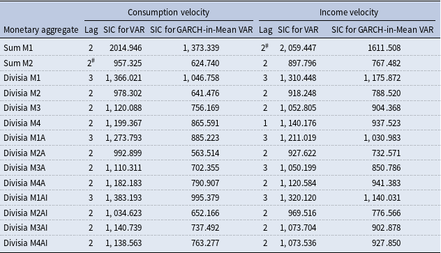
Model specification tests for the GARCH-in-mean VAR

Table 5 Long description
A table comparing model specification tests for GARCH-in-mean VAR across different monetary aggregates. The table has 16 rows and 6 columns. The columns are labeled as follows: Monetary aggregate, Lag, SIC for VAR, SIC for GARCH-in-Mean VAR, Lag, SIC for VAR, SIC for GARCH-in-Mean VAR. The rows are labeled with different monetary aggregates: Sum M1, Sum M2, Divisia M1, Divisia M2, Divisia M3, Divisia M4, Divisia M1A, Divisia M2A, Divisia M3A, Divisia M4A, Divisia M1AI, Divisia M2AI, Divisia M3AI, Divisia M4AI. Each row provides values for the lag, SIC for VAR, and SIC for GARCH-in-Mean VAR for both consumption velocity and income velocity. Notable trends include varying lag selections and SIC values across different monetary aggregates. The table also includes notes on the sample period and lag selection criteria.
Notes: The sample period is 2006:m7 to 2025:m6.
Lags are selected based on minimum SIC value for the conventional VAR.
 $^\#$
Lag is selected among twelve lags based on the minimum SIC for conventional VAR subject to stable GARCH-in-Mean VAR.
Tables 5 and 6 summarize the estimates from the GARCH-in-Mean VAR using both the consumption and income velocity of money. The tables document model specification tests based on the SIC for each monetary aggregate. We select the lag length based on the minimum SIC from the conventional VAR associated with each stable (i.e. model with convergence) GARCH-in-Mean VAR model. Thus, the optimal lag is chosen from the convergent GARCH-in-Mean VAR specifications. Using the consumption velocity, we select a lag length of 2 with the Sum M1 and Sum M2 aggregates, as reported in the second column of Table 5. Similarly, we select a lag length of 2 for all of the (original, credit card-augmented, and credit card-augmented inside) Divisia M2, Divisia M3, and Divisia M4 aggregates. A lag length of 3 is selected for the narrow (at the M1 level of aggregation) Divisia aggregates.
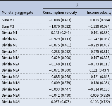
GARCH-in-mean VAR
 $\lambda$
coefficient estimates

Table 6 Long description
A table comparing GARCH-in-mean VAR lambda coefficient estimates for different monetary aggregates. The table has 16 rows and 3 columns. The columns are labeled ’Monetary aggregate’, ’Consumption velocity’, and ’Income velocity’. Each row lists a different monetary aggregate and its corresponding lambda coefficient estimates with p-values in parentheses. The monetary aggregates include Sum M1, Sum M2, Divisia M1, Divisia M2, Divisia M3, Divisia M4, Divisia M1A, Divisia M2A, Divisia M3A, Divisia M4A, Divisia M1AI, Divisia M2AI, Divisia M3AI, and Divisia M4AI. The table provides estimates for both consumption velocity and income velocity. Notable trends include varying lambda coefficient estimates and p-values across different monetary aggregates.
Notes: The sample period is 2006:m7 to 2025:m6.
Numbers in parentheses are p-values.
The third and fourth columns of Table 5 report the SIC values for the conventional VAR and the GARCH-in-Mean VAR, respectively. For each aggregate and selected lag, the GARCH-in-Mean VAR yields a lower SIC than the conventional VAR when using the consumption velocity, underscoring the superiority of the structural GARCH-in-Mean VAR model over the conventional VAR. After fixing the lag length, we estimate the GARCH-in-Mean VAR to identify the coefficient capturing the effect of money growth volatility on the consumption velocity, denoted by
 $\lambda$
. The second column of Table 6 reports the estimates of
 $\lambda$
and
 $p$
-values for the null hypothesis
 $H_{0} \, : \, \hat {\lambda }=0$
. The coefficients are statistically significant at the 5% level only with the Sum M2 aggregate (
 $\hat {\lambda }=-1.070$
with a
 $ p$
-value of
 $0.022$
) and the Divisia M1A aggregate (
 $\hat {\lambda }=-0.029$
with a
 $p$
-value of
 $0.000$
), with the negative signs indicating the negative effect of monetary volatility on the velocity of money.
We repeat the analysis using the income velocity of money. The corresponding results appear in columns five to seven of Table 5 and the third column of Table 6. The fifth column of Table 5 shows that the selected lag length for the Sum M1 and Sum M2 aggregates remains 2, matching the specifications based on the consumption velocity. As in the corresponding consumption velocity-based specifications, the same lag length of 2 also applies to Divisia M2, Divisia M3, Divisia M2A, Divisia M4A, and all the augmented Divisia inside aggregates; the optimal lag length for Divisia M1, Divisia M1A, Divisia M3A, and Divisia M1AI is 3, and that for Divisia M4 is 1, differing from the consumption-based specifications. Nevertheless, the SIC values in the sixth and seventh columns of Table 5 indicate that the GARCH-in-Mean VAR outperforms the conventional VAR for all aggregates.
After fixing the lag length, we estimate the model using the income velocity of money. The estimated
 $\lambda$
coefficients in the third column of Table 6 show that at the 5% level of significance money growth volatility has no statistically significant effect on the income velocity for any of the monetary aggregates. This result broadly aligns with the findings based on the consumption velocity of money, and we conclude that the structural model provides strong evidence against Friedman’s hypothesis that monetary variability affects the velocity of money.
4.3 Robustness
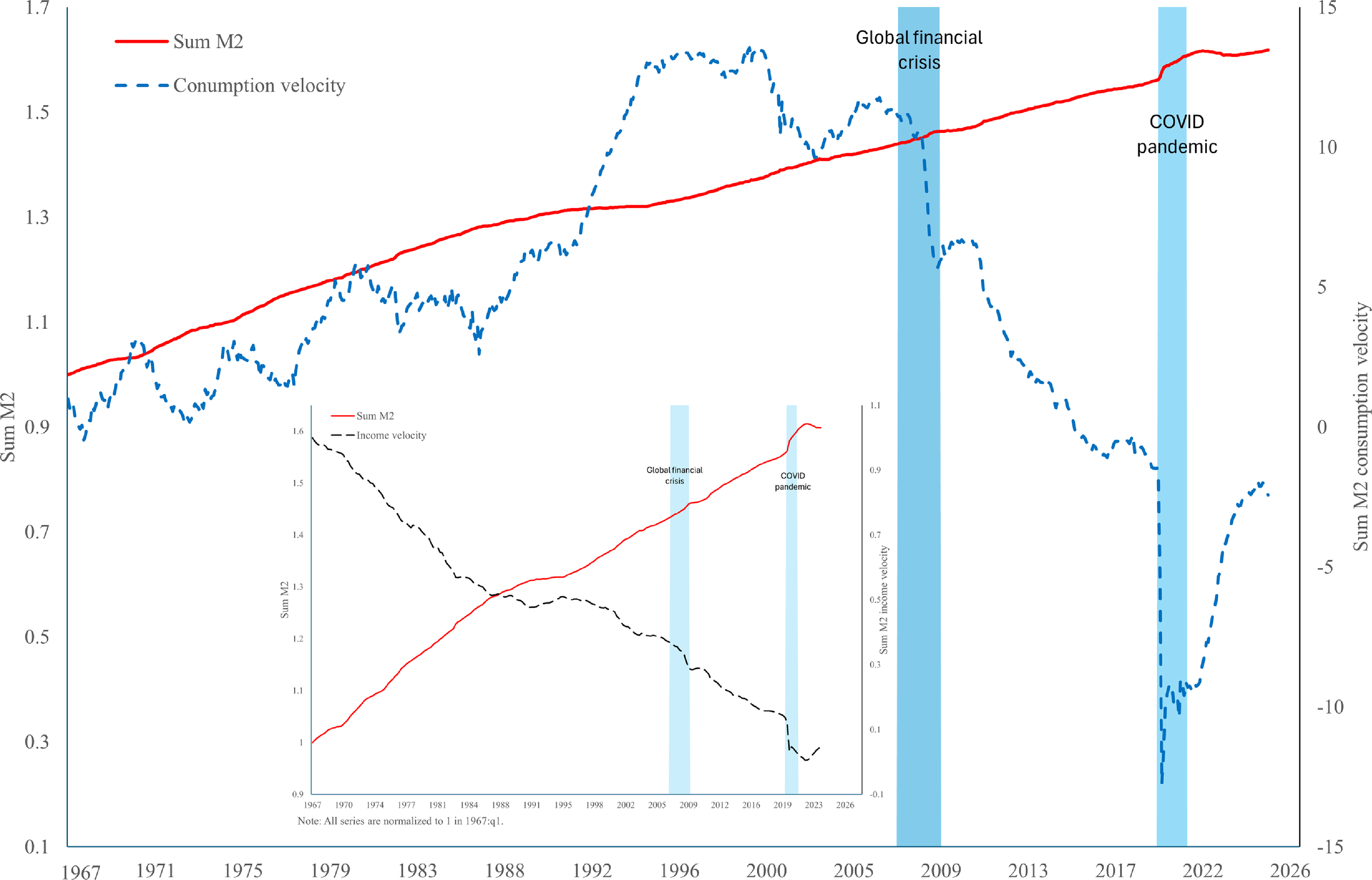
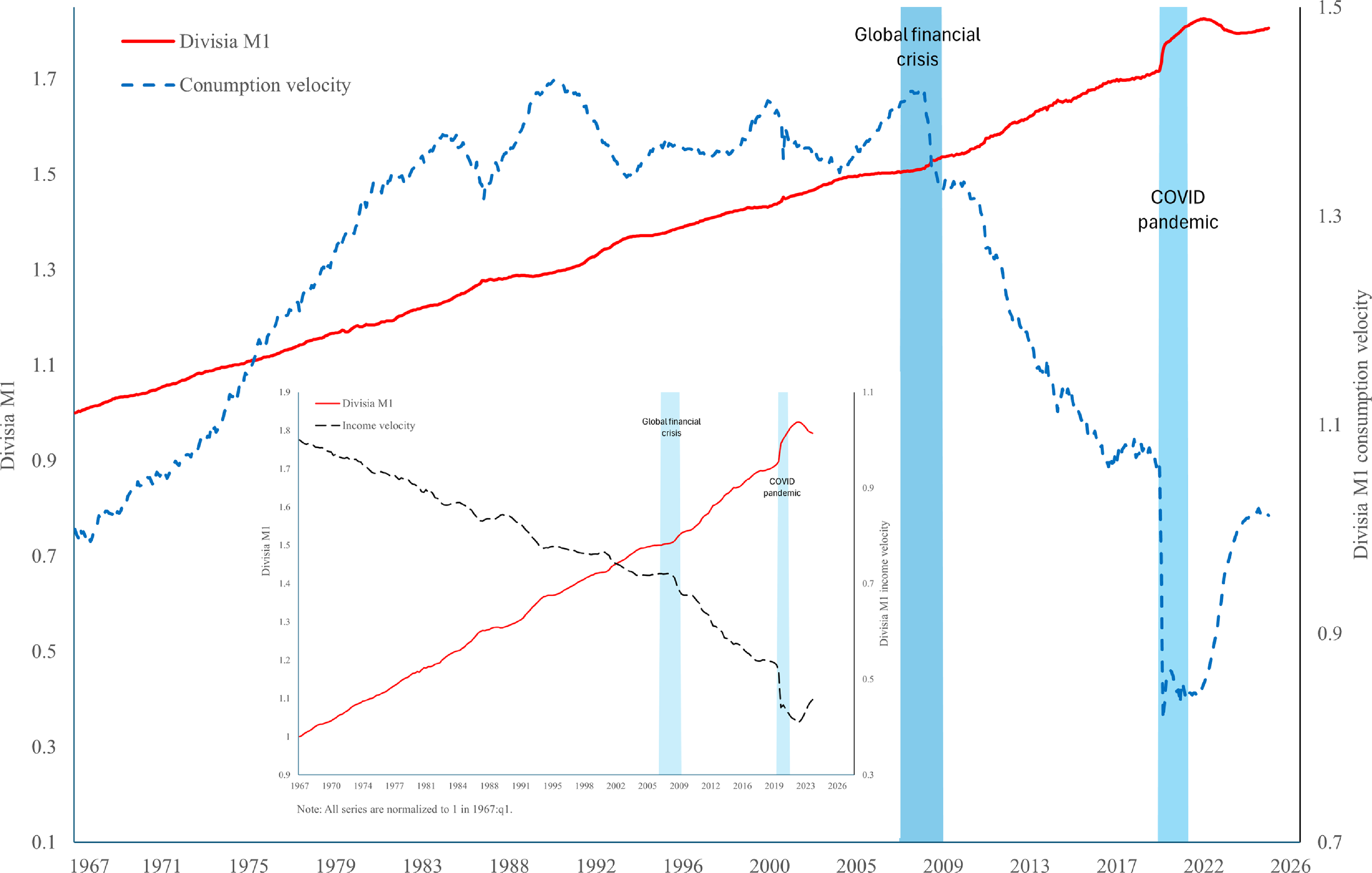
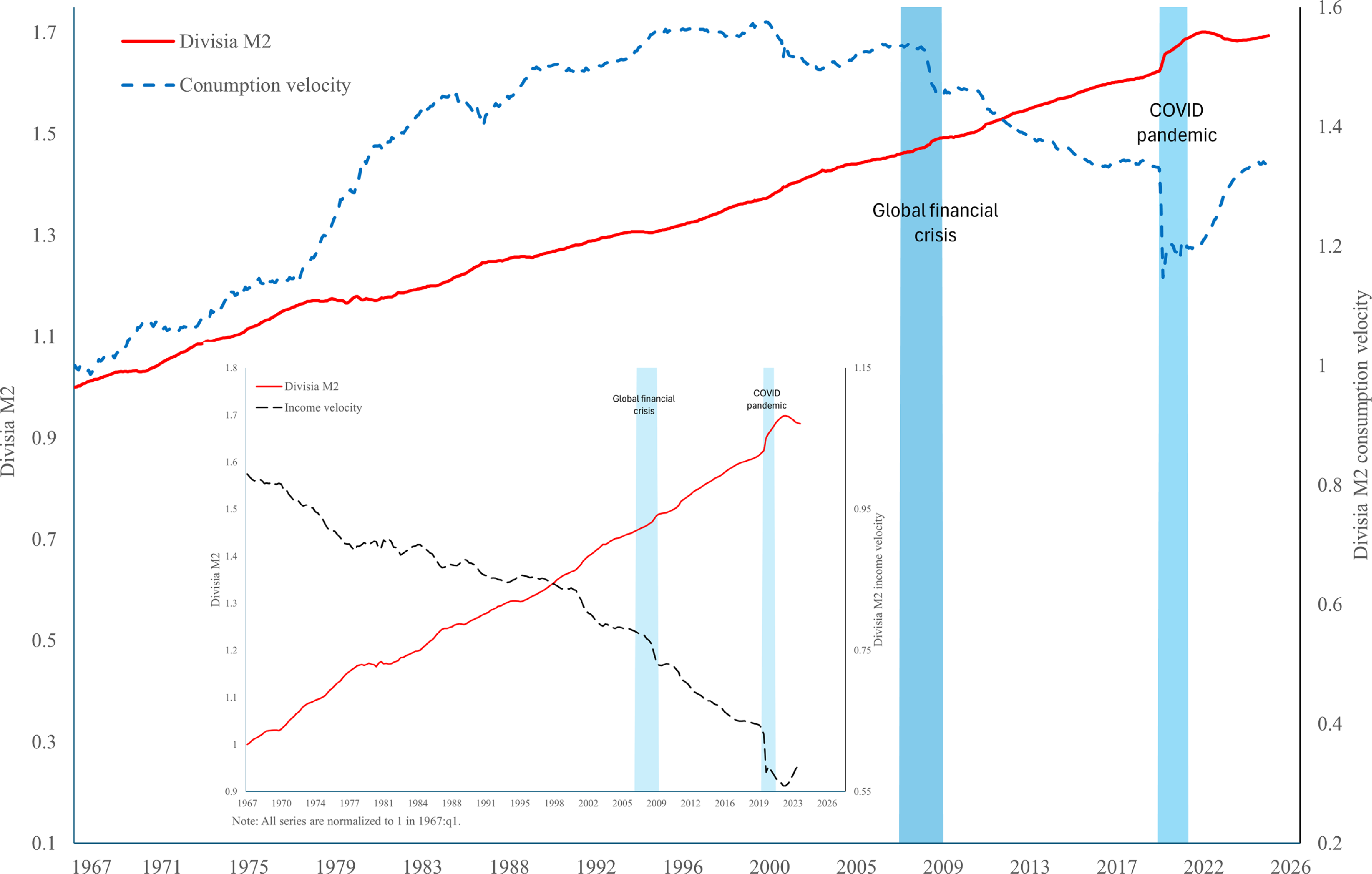
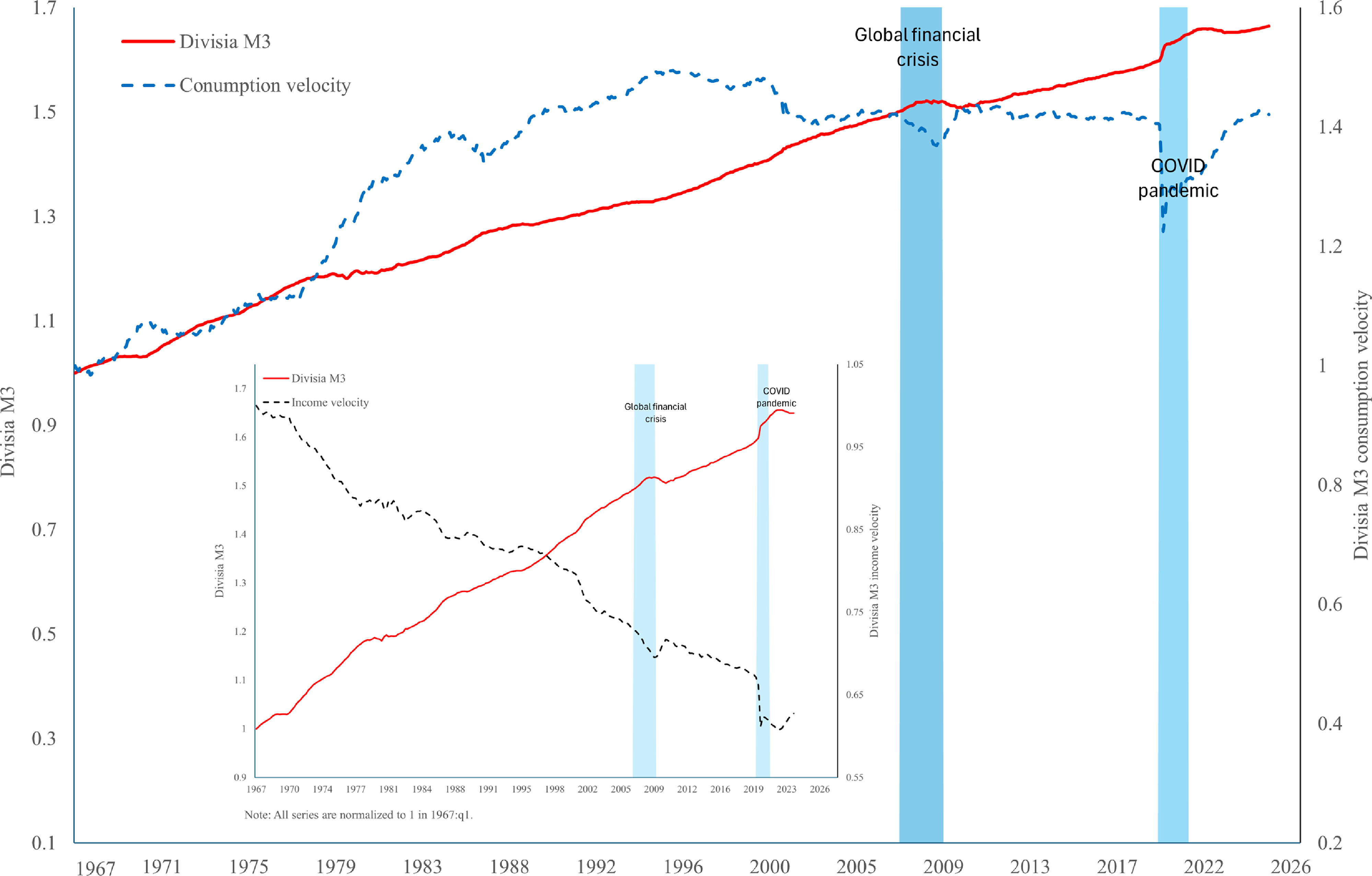
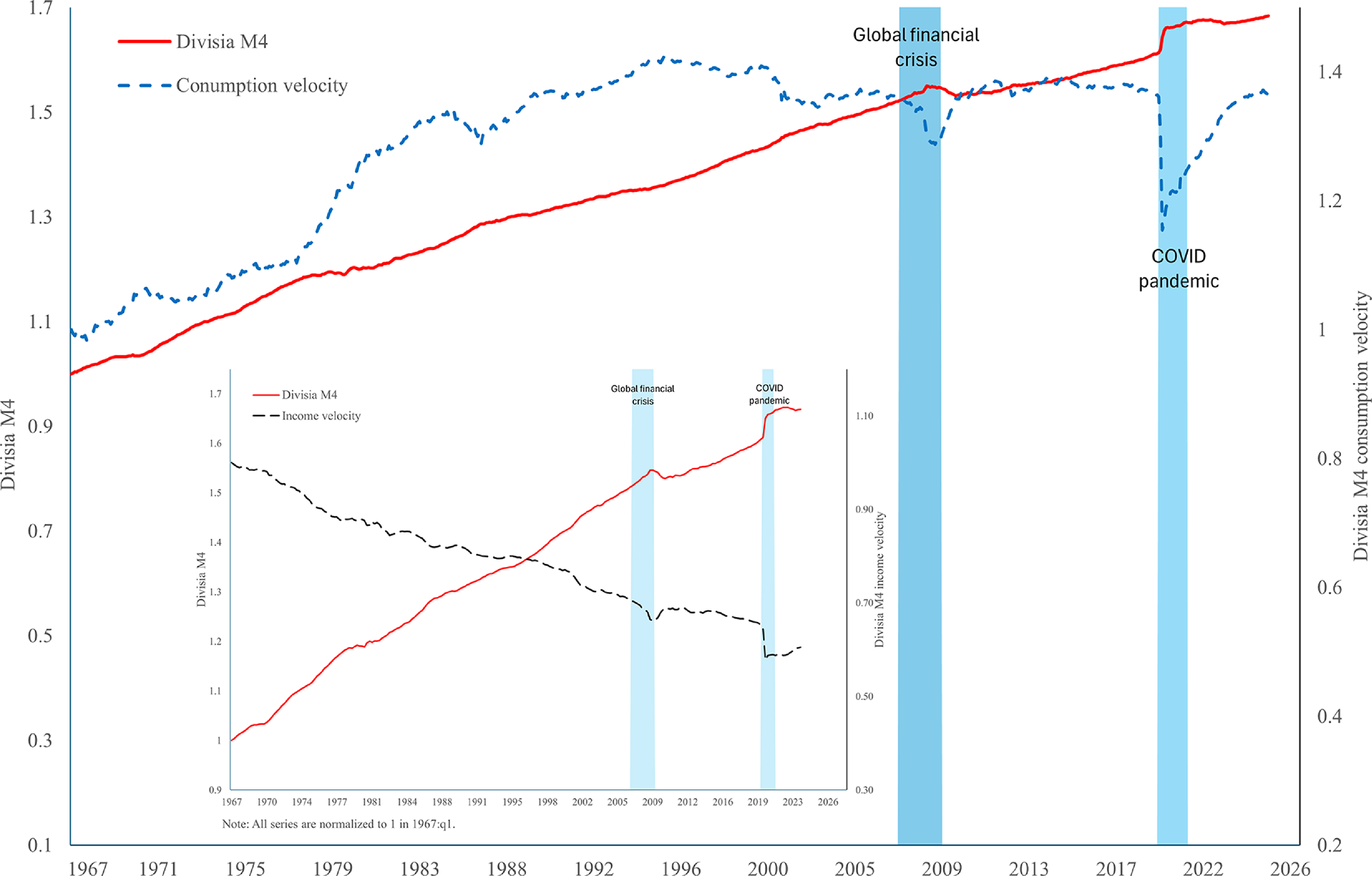
In the analysis so far we used monthly data over the period from 2006:m7 to 2025:m6 for which all monetary aggregates are available. Since the simple-sum aggregates and the original Divisia aggregates are available since 1967:m1, in this section we use a longer sample. However, because the monthly NGDP index from S&P Global Market Intelligence that we used in the previous section to construct the income velocity of money is not available over this longer period, we use quarterly data and a real GDP series from FRED to construct the income velocity of money. Thus, in doing so, we investigate the robustness of our results to the use of a longer sample using the consumption velocity of money (over the period from 1967:m1 to 2025:m6) and also to the use of quarterly data using the income velocity of money based on real GDP (over the period from 1967:q1 to 2025:q2). It is to be noted that this longer sample, and the comparison between the simple-sum aggregates and the original Divisia aggregates, attracted most of the attention so far in the literature. Figures 15–20 show the logged monetary aggregates (Sum M1, Sum M2, Divisia M1, Divisia M2, Divisia M3, and Divisia M4, respectively) together with their corresponding consumption and income velocities, in the same fashion as in Figures 1–14.
The logged Sum Ml aggregate and its consumption and income velocities since 1967.
Note: All series are normalized to 1 in 1967 ml.

The logged Sum M2 aggregate and its consumption and income velocities since 1967.
Note: All series are normalized to 1 in 1967 ml.

The logged Divisia Ml aggregate and its consumption and income velocities since 1967.
Note: All series are normalized to 1 in 1967 ml.

Figure 17. Long description
The image contains two line graphs. The main graph shows the Divisia M1 aggregate and consumption velocity over time from 1967 to 2026. The horizontal axis represents the years, while the left vertical axis represents the Divisia M1 values and the right vertical axis represents the Divisia M1 consumption velocity. The red solid line represents the Divisia M1 aggregate, and the blue dashed line represents the consumption velocity. Key events such as the Global financial crisis and the COVID pandemic are highlighted with vertical blue bands. The inset graph shows the Divisia M1 aggregate and income velocity over the same period. The horizontal axis represents the years, while the left vertical axis represents the Divisia M1 values and the right vertical axis represents the Divisia M1 income velocity. The red solid line represents the Divisia M1 aggregate, and the black dashed line represents the income velocity. The graphs illustrate the trends and relationships between these economic indicators over time.
The logged Divisia M2 aggregate and its consumption and income velocities since 1967.
Note: All series are normalized to 1 in 1967 ml.

The logged Divisia M3 aggregate and its consumption and income velocities since 1967.
Note: All series are normalized to 1 in 1967 ml.

Figure 19. Long description
The image contains two line graphs. The first graph shows the Divisia M3 aggregate and consumption velocity over time from 1967 to 2026. The x-axis represents the years, and the y-axis on the left represents the Divisia M3 values, while the y-axis on the right represents the consumption velocity. The red solid line represents the Divisia M3 aggregate, and the blue dashed line represents the consumption velocity. Key events such as the Global financial crisis and the COVID pandemic are highlighted with vertical blue bars. The second graph, inset within the first, shows the Divisia M3 aggregate and income velocity over the same period. The x-axis represents the years, and the y-axis on the left represents the Divisia M3 values, while the y-axis on the right represents the income velocity. The red solid line represents the Divisia M3 aggregate, and the black dashed line represents the income velocity. The graphs illustrate the trends and relationships between the Divisia M3 aggregate, consumption velocity, and income velocity over time, highlighting significant economic events.
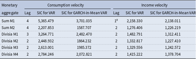
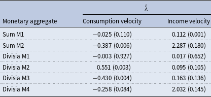
We estimate the GARCH-in-Mean VAR (in the same fashion as in the previous section) and report the results in Tables 7 and 8. With the monthly data and the consumption velocity of money, the selected lag length is 4 for both Sum M1 and Sum M2, 3 for Divisia M1, and 2 for each of Divisia M2, Divisia M3, and Divisia M4. With the quarterly data and the income velocity of money, the selected lag length is 1 for Sum M1 and 2 for all of the other aggregates. Table 7 also shows that the structural specification outperforms the conventional VAR across all monetary aggregates considered for both the monthly and quarterly data. Finally, Table 8 indicates a negative and statistically significant (at the 5% level) effect of money growth variability on the consumption velocity of money only with the Sum M2 (
 $\hat { \lambda }=-0.387$
with a
 $p$
-value of
 $0.006$
) and Divisia M3 (
 $\hat {\lambda } =-0.430$
with a
 $p$
-value of
 $0.004$
) aggregates. We find no negative and statistically significant effect with the quarterly data and the income velocity of money.
Model specification tests for the GARCH-in-mean VAR for the 1967–2025 sample

Table 7 Long description
A table comparing model specification tests for GARCH-in-mean VAR across different monetary aggregates. The table has two main sections: Consumption velocity and Income velocity, each with three columns: Lag, SIC for VAR, and SIC for GARCH-in-Mean VAR. The rows are labeled with different monetary aggregates: Sum M1, Sum M2, Divisia M1, Divisia M2, Divisia M3, and Divisia M4. Row 1: Sum M1, Lag 4, SIC for VAR 5,365.479, SIC for GARCH-in-Mean VAR 3,701.035, Lag 1, SIC for VAR 2,158.330, SIC for GARCH-in-Mean VAR 2,138.011. Row 2: Sum M2, Lag 4, SIC for VAR 2,207.853, SIC for GARCH-in-Mean VAR 1587.707, Lag 2, SIC for VAR 1,276.406, SIC for GARCH-in-Mean VAR 1,226.219. Row 3: Divisia M1, Lag 3, SIC for VAR 3,264.771, SIC for GARCH-in-Mean VAR 2,482.470, Lag 2, SIC for VAR 1,482.791, SIC for GARCH-in-Mean VAR 1,312.411. Row 4: Divisia M2, Lag 2, SIC for VAR 2,448.932, SIC for GARCH-in-Mean VAR 1864.232, Lag 2, SIC for VAR 1,332.817, SIC for GARCH-in-Mean VAR 1,227.410. Row 5: Divisia M3, Lag 2, SIC for VAR 2,613.001, SIC for GARCH-in-Mean VAR 1985.372, Lag 2, SIC for VAR 1,329.556, SIC for GARCH-in-Mean VAR 1,242.572. Row 6: Divisia M4, Lag 2, SIC for VAR 2,784.246, SIC for GARCH-in-Mean VAR 2,072.821, Lag 2, SIC for VAR 1,415.222, SIC for GARCH-in-Mean VAR 1,378.704.
Notes: The sample period with the consumption velocity is 1967:m1 to 2025:m6 and that with the income velocity is 1967:q1 to 2025:q2.
Lags are selected based on the minimum SIC value for the conventional VAR.
 $^\#$
Lag is selected among twelve lags based on the minimum SIC for conventional VAR subject to stable GARCH-in-Mean VAR.
The logged Divisia M4 aggregate and its consumption and income velocities since 1967.
Note: All series are normalized to 1 in 1967 ml.

5. Conclusion
In this paper we investigate the Friedman hypothesis that the variability of money growth affects the velocity of money. We use standard Granger causality tests and (for the first time) a bivariate structural GARCH-in-Mean VAR model to examine how money growth variability affects the consumption and income velocity of money. We make comparisons among the two simple-sum monetary aggregates published by the Federal Reserve and the original (non-credit-card-augmented) Divisia monetary aggregates, the credit card-augmented Divisia aggregates, and the credit card-augmented Divisia inside aggregates. We use monthly data over the post-2006 period, for which all monetary indicators are available, but also investigate the robustness of our results to a longer sample for which the original Divisia aggregates are available and also to the use of quarterly data (going back to 1967).
GARCH-in-mean VAR
 $\lambda$
coefficient estimates with the 1967–2025 sample

Table 8 Long description
A table comparing GARCH-in-mean VAR coefficient estimates for different monetary aggregates. The table has 8 rows and 5 columns. The columns are labeled ’Monetary aggregate’, ’Consumption velocity’, and ’Income velocity’. The ’Consumption velocity’ column has two sub-columns labeled with lambda symbol and its p-value. The ’Income velocity’ column also has two sub-columns labeled with lambda symbol and its p-value. The rows are labeled with different monetary aggregates: Sum M1, Sum M2, Divisia M1, Divisia M2, Divisia M3, and Divisia M4. Row 1: Sum M1, -0.025 (0.110), 0.112 (0.001). Row 2: Sum M2, -0.387 (0.006), 2.287 (0.180). Row 3: Divisia M1, -0.003 (0.927), 0.017 (0.652). Row 4: Divisia M2, 0.551 (0.003), 0.095 (0.105). Row 5: Divisia M3, -0.430 (0.004), 0.163 (0.136). Row 6: Divisia M4, -0.258 (0.084), 2.032 (0.145). The table shows the lambda coefficient estimates and their p-values for both consumption velocity and income velocity across different monetary aggregates.
Notes: The sample period with the consumption velocity is 1967:m1 to 2025:m6 and that with the income velocity is 1967:q1 to 2025:q2.
Numbers in parentheses are p-values.
Our findings indicate that the Friedman hypothesis can be rejected if money supply volatility is modeled explicitly using recent advances in macroeconometrics and financial econometrics. In particular, the evidence from the structural GARCH-in-Mean VAR model indicates a weak effect of uncertainty associated with money growth on the velocity of money, irrespective of how money and velocity are measured. This finding has important implications for the role of money in the conduct of monetary policy, as it suggests that velocity remains stable in the presence of money growth uncertainty. Consequently, monetary aggregates may potentially be used to generate predictable changes in real output and guide output dynamics. This is consistent with Belongia and Ireland (Reference Belongia and Ireland2015, pp. 268) who “call into question the conventional view that the stance of monetary policy can be described with exclusive reference to its effects on interest rates and without consideration of simultaneous movements in the monetary aggregates.” It also reinforces the argument by Serletis (Reference Serletis2025, pp. 117) that “ there is a meaningful role for properly measured monetary aggregates in dynamic stochastic general equilibrium models, and that central banks around the world could achieve more favorable macroeconomic outcomes by paying attention to these monetary aggregates.”
Acknowledgements
This paper builds on material from Chapter 2 of Md Maidul Islam Chowdhury’s Ph.D. dissertation at the University of Calgary. We would like to thank Bill Barnett, Fredj Jawadi, two anonymous referees, and the members of Maidul’s dissertation committee, Atsuko Tanaka and Sonja Chen.
Statements and declarations
We haven’t used AI tools.
Competing interests
We have no conflicts of interest.
 λ
 λ

 Open access

