


1. Introduction: The Problem of understanding Surge Progression in a Large, Complex Glacier System
Understanding acceleration in glaciers and fast-glacier movement is essential to understanding changes in the cryosphere. Glacier surging is one of three types of fast glacier flow (Reference ClarkeClarke, 1987) – ice streams, surging, and tidewater glaciers – and the one that has been least researched. This paper is dedicated to designing an approach that facilitates objective analysis and parameterization of surge progression in a large and complex glacier system, using observations of the current surge of the Bering–Bagley glacier system, Alaska, USA.
A surge is a catastrophic dynamic event, during which a glacier accelerates to 10–100 times or more of its normal velocity and advances rapidly. Heavy crevassing indicative of sudden deformation, horizontal and vertical displacement of ice and sudden changes in the glacial hydrologic system are characteristics of a surge. The contemporary state of knowledge on the surge process was summarized by Reference Meier and PostMeier and Post (1969), Reference RaymondRaymond (1987) and Reference Harrison and PostHarrison and Post (2003), who each concluded that the physics of the surge process were still not understood. It is known that a surge glacier builds up ice in a reservoir area during the long, quiescent phase of the surge, and this ice is then rapidly released during the surge phase. The kinematic wave associated with the surge travels up-glacier and down-glacier. Surges occur in several stages (Reference Herzfeld and MayerHerzfeld and Mayer, 1997; Reference HerzfeldHerzfeld, 1998). In recent studies, the effects of glacier geometry, climate and setting, of basal morphology and composition of the bed, or rather, susceptibility of the bed material to deformation, and of englacial water distribution have been investigated in three respects: as factors that may explain that a given glacier is a surge-type glacier; as causes of glacier surges; and as triggers of an actual surge (Reference Björnsson, Palsson, Sigurðsson and FlowersBjörnsson and others, 2003; Reference Copland, Sharp and DowdeswellCopland and others, 2003; Reference Fatland, Lingle and TrufferFatland and others, 2003; Reference Harrison and PostHarrison and Post, 2003; Reference Jiskoot, Murray and LuckmanJiskoot and others, 2003; Reference Lingle and FatlandLingle and Fatland, 2003; Reference Murray, Luckman, Strozzi and NuttallMurray and others, 2003; cf. Reference Bruhn, Forster, Ford, Pavlis, Vorkink, Shuchman and JosbergerBruhn and others, 2010).
Moreover, much of the research on the physics of the surge process is based on a few case studies of mostly smaller glaciers, such as the 1982/83 surge of Variegated Glacier, Alaska (e.g. Reference KambKamb and others, 1985; Reference Humphrey, Raymond and HarrisonHumphrey and others, 1986; Reference RaymondRaymond, 1987), and surges of Trapridge Glacier, Yukon, Canada (Reference Clarke, Collins and ThompsonClarke and others, 1984; Reference Flowers and ClarkeFlowers and Clarke, 2000, Reference Flowers and Clarke2002a,Reference Flowers and Clarkeb), which are easier to equip with geophysical instrumentation but behave differently than large glaciers. Reference Meier and PostMeier and Post (1969) distinguish three types of surging glaciers: (1) large-sized with high surge velocities, large displacement and large lowering of ice reservoir; (2) large-sized with low surge velocities and small vertical and horizontal ice displacement; and (3) steep and small-sized with small reservoir lowering and ice displacement. The progression of a surge in a large glacier and the characteristic dynamics of each surge phase have not been analyzed systematically.
Bering Glacier, Alaska, is a prototype of a large surge-type glacier of type 1 , whose size is comparable to large fast-moving ice streams in Greenland, which individually play a role in understanding ice-sheet stability and discharge into the ocean. Bering Glacier is also the largest temperate surge-type glacier on Earth. The surge of Bering Glacier progresses into the Bagley Ice Field (Reference HerzfeldHerzfeld, 1998; Reference MolniaMolnia, 2001, Reference Molnia, Williams and Ferrigno2008; Reference Fatland, Lingle and TrufferFatland and others, 2003; Reference Molnia, Post, Shuchman and JosbergerMolnia and Post, 2010a,Reference Molnia, Post, Shuchman and Josbergerb). Therefore the current surge of the Bering–Bagley system provides a good opportunity to contribute to our understanding of the physics of the surge process in a large and complex glacier system, as well as for research on exemplary processes of ice acceleration in general.
Observing, analyzing and understanding the surge progression in a large glacier requires a different method than measurement of geophysical properties on the ice, because it is not practical to instrument a large glacier. The approach used here is a form of automated spatial analysis of airborne remote-sensing data. The idea is based on the notion that rapid movement of ice manifests itself in crevassing, and that crevasses are associated with deformation provinces in a consistent manner. We establish that this relationship is sufficient to associate surge kinematics/deformation types from imagery collected over a glacier during surge.
Remote-sensing data analysis has been applied in research on the last surge of Bering Glacier (1993–95), resulting in valuable velocity measurements, documentation of front advance and qualitative descriptions of components of the surge process (Reference Fatland, Lingle and TrufferFatland and others, 2003; Reference Roush, Lingle, Guritz, Fatland and VoroninaRoush and others, 2003; Reference Molnia, Post, Shuchman and JosbergerMolnia and Post, 2010b; Reference Shuchman, Josberger, Jenkins, Payne, Hatt, Spaete, Shuchman and JosbergerShuchman and others, 2010). For example, Reference Lingle and FatlandLingle and Fatland (2003) suggest a possible progression qualitatively (in summary, water needs to be stored in a distributed system in the glacier but then the actual surge may be triggered by meteorologic events).
Remote-sensing data analysis of Bering Glacier or any other (large) surge-type glacier has not yet been linked to a physical process model. This requires a discretization and parameterization of kinematic and dynamic processes. In this paper, we describe how automated image analysis and classification can be applied to derive the dynamics of the surge progression during early, mature and late surge stages. The classification yields a set of parameters that capture components of the dynamics of surge progression. The analysis and classification of crevassed ice surfaces from images collected during the current (2011) surge of the Bering-Bagley glacier system forms a central part of the paper. The vertical component of the surge kinematics can be constrained using analysis of laser altimeter data (Reference Herzfeld, McDonald, Stachura, Griffin Hale and Chen Pand TrantowHerzfeld and others, 2013).
2. The Surge of the Bering-Bagley Glacier System in 2011
In late spring 2011, Bering Glacier (Fig. 1) started to show definite signs of a surge. Bering Glacier is the largest (∼5200km2) and longest (∼200km) glacier in North America (Reference Molnia, Williams and FerrignoMolnia, 2008, p. K203); its accumulation zone includes the Bagley Ice Valley and Columbus Glacier. During a surge, Bering Glacier advances into and over a series of proglacial lakes very close to the Gulf of Alaska (Reference PostPost, 1960, Reference Post1972; Reference Molnia and PostMolnia and Post, 1995a; Reference HerzfeldHerzfeld, 1998; Reference MolniaMolnia, 2001). As a result of the advance, the surge affects the ecological balance in the environment surrounding the glacier and potentially threatens shipping lanes through iceberg calving, so understanding the surge is important not only as a glaciological phenomenon, but also for the environment and society.
En-échelon crevasses in Bagley Ice Field; reopening caused by surge progression after recent snowfall, 25 September 2011.

Bering Glacier last surged in 1993-95 (Reference PostPost, 1972; Reference Lingle, Post, Herzfeld, Molnia, Krimmel and RoushLingle and others, 1993; Reference Molnia and PostMolnia and Post, 1995, Reference Molnia, Post, Shuchman and Josberger2010b; Reference Herzfeld and MayerHerzfeld and Mayer, 1997; Reference Fatland and LingleFatland and Lingle, 1998; Reference HerzfeldHerzfeld, 1998; Reference Mayer and HerzfeldMayer and Herzfeld, 2000; Reference MolniaMolnia, 2001, Reference Molnia, Williams and Ferrigno2008; Reference Lingle and FatlandLingle and Fatland, 2003; Reference Roush, Lingle, Guritz, Fatland and VoroninaRoush and others, 2003; Reference Fleisher, Bailey, Natel, Muller, Cadwell, Russell, Shuchman and JosbergerFleisher and others, 2010; Reference Josberger, Shuchman, Meadows, Savage, Payne, Shuchman and JosbergerJosberger and others, 2010; Reference Shuchman and JosbergerShuchman and Josberger, 2010; Reference Shuchman, Josberger, Jenkins, Payne, Hatt, Spaete, Shuchman and JosbergerShuchman and others, 2010). The geography of Bering Glacier-Bagley Ice Valley, with place names, is described in Reference Molnia, Post, Shuchman and JosbergerMolnia and Post (2010a).
The current surge was preceded by a weak surge-type acceleration which started in 2008 and stopped in the same year. In 2009, no surge dynamics was observed, and in 2010 no observations were made (personal communication from B. Molnia, 2011). In early 2011, Bering Glacier’s dynamics suddenly changed to that of a full-scale surge, with deformations and dynamics different than the previous surge. The surge started in lower central Bering Glacier on the northwestern side and soon reached the ice front in Tashalich arm (by May 2011). The 1993-95 surge started in a similar location (Reference HerzfeldHerzfeld, 1998; Reference Roush, Lingle, Guritz, Fatland and VoroninaRoush and others, 2003). The surge progressed up-glacier, as indicated by large, discrete crevasse fields separated by extensive regions of uncrevassed ice. By 25 September 2011, the surge had advanced into the Bagley Ice Field to 141°59‘W. Fresh en-echelon crevasse fields opened at several locations near the feet of topographic spurs that suggest subglacial morphologic induction (for an explanation, see Section 6). Judging by the clear-cut shapes of the crevasse fields, these must have opened only a few days before survey (Fig. 1). In 1994, surge crevassing had affected the entire Bering Glacier (Reference HerzfeldHerzfeld, 1998), while in 2011 large parts of Bering Glacier continued to show ductile deformation typical of the quiescent phase, at a time when the surge kinematics had already progressed into the Bagley Ice Field.
3. Approach: Structural Glaciological Provinces
An essential component of the crevasse classification is the observation that crevasses occur in large areas of similar crevasse patterns with clear boundaries to the neighboring areas of crevasses. This motivates use of the terminology of a structural province. A structural province is a region of a glacier that is homogeneous with respect to structural glaciological properties and that is maximal with this property. For instance, for a crevassed glacier, a structural province is an area that is maximal with the property of including the same crevasse type. The goal of the crevasse classification to be discussed in this paper is to utilize crevasse patterns derived from image data as a source of geophysical information. That this is conceptually possible is explained as follows.
The principal concept is that the dynamics of fast-moving ice manifest themselves in crevassing, so the deformation history of the ice can be reconstructed by analysis of crevasse patterns. Structural geological principles provide links between dynamics, kinematics and deformation, which can be physically formalized and quantified using continuum mechanics (Reference MeansMeans, 1976; Reference SuppeSuppe, 1985; Reference Twiss and MooresTwiss and Moores, 1992; Reference Ramsay and LisleRamsay and Lisle, 2000; Reference LiuLiu, 2002; Reference GreveGreve, 2003). Crevassing is a form of brittle deformation that occurs when local forces exceed a threshold. Characterization of generalized spatial surface roughness is a mathematical approach that utilizes parameters derived from spatial statistical functions to capture spatial properties of a surface (Reference HerzfeldHerzfeld, 2008). This applies to crevassed and non-crevassed ice surfaces. Combining structural geology and mathematical roughness analysis allows the derivation of deformation characteristics in fast-moving glaciers, as described in theory in Reference Herzfeld, Clarke, Mayer and GreveHerzfeld and others (2004), and the mapping of deformation provinces in surging and continuously fast-moving glaciers (Reference Herzfeld and MayerHerzfeld and Mayer, 1997; Reference HerzfeldHerzfeld, 1998; Reference Herzfeld, Mayer, Feller and MimlerHerzfeld and others, 2000; Reference Mayer and HerzfeldMayer and Herzfeld, 2000, Reference Mayer and Herzfeld2001, Reference Mayer and Herzfeld2008; Reference Herzfeld and ZahnerHerzfeld and Zahner, 2001; cf. Reference Vornberger and WhillansVornberger and Whillans, 1990; Reference Marmo and WilsonMarmo and Wilson, 1998; Reference RistRist and others, 1999).
Reference HopkinsHopkins (1862) gave an early explanation of crevasse patterns by applying stress analysis to the distribution of stress in a continuously deforming body. Mathematical description of the mechanical properties of glacier flow goes back to Reference NyeNye (1952), who introduced the terms ‘compressive flow’ and ‘extensive flow’ and addressed the theoretical positions and directions of crevasses dependent on local stress fields (fig. 9 in Reference NyeNye, 1952). Reference NyeNye (1952) is concerned with the case of ductile deformation or continuous flow. Sudden changes in force typically accompany a surge and cause characteristic brittle deformation, which may be viewed as discretized flow or deformation events. The deformation events lead to fields of clear-cut crevasses. The different appearances of crevasse fields resulting from continuous deformation and discrete deformation are illustrated in a comparison of crevasse types of Jakobshavn Isbræ, Greenland, and Bering Glacier (Reference Mayer and HerzfeldMayer and Herzfeld, 2000); mathematical differences are discussed in Reference Herzfeld, Clarke, Mayer and GreveHerzfeld and others (2004).
4. Observations
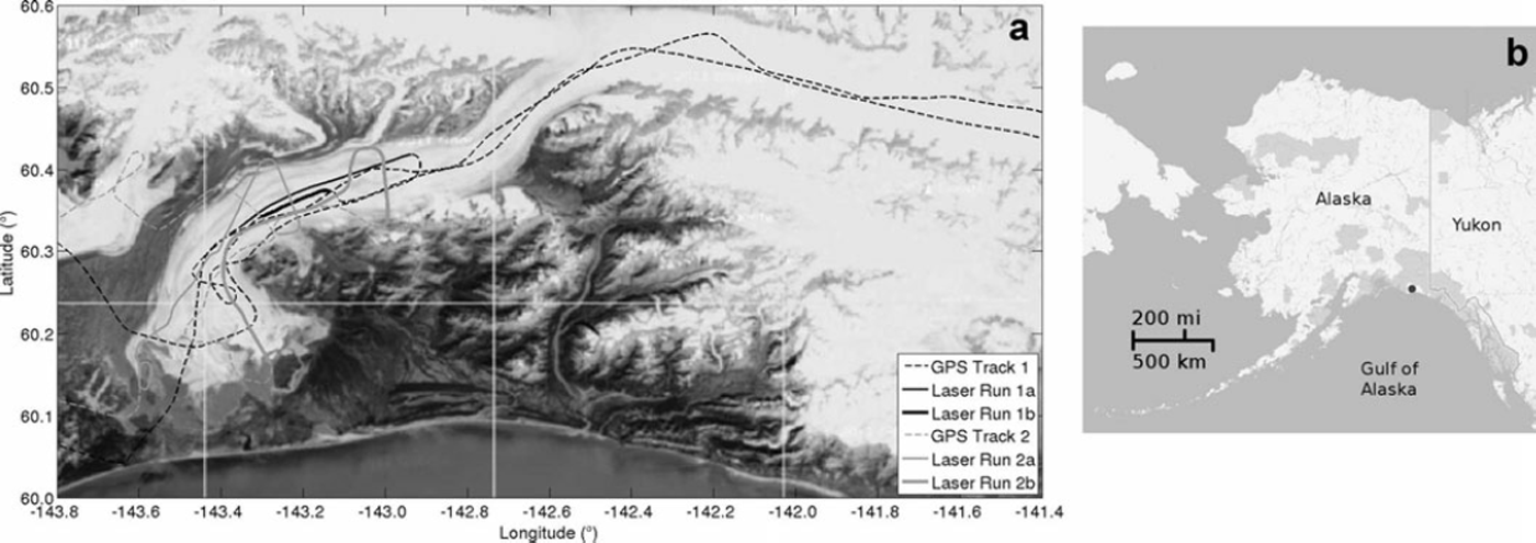
Digital photographic data, digital video data, GPS data and laser altimeter data were collected over the Bering–Bagley glacier system during an aerial observation campaign in September 2011. Data were collected along pre-planned flight lines, which include lines that approximately follow the flowline and several lines that are perpendicular to the flowline (Fig. 2). The analysis presented here is based on airborne digital image data, referenced to position by GPS data of the plane’s position. Although the pointing angle of the camera is only known with the accuracy of a handheld camera and aircraft motion was not recorded (other than by the flight-track GPS coordinates), the concept of structural provinces and the large size of these provinces assists with correctly associating deformation types to location. Satellite data from Digital Globe (WorldView) and the Geodetic and Earth Observing Satellite (GEOS) are also available, but there are no data that provide complete coverage of the glacier system at any point in time during the surge in 2011. For example, for a composition of WorldView imagery covering the entire Bering Glacier and Bagley Ice Valley, six images are needed and a set includes data from several different months. In comparison, the video and photographic image data collected during a single observation flight provide images of the glacier from the calving front to the upper Bagley Ice Valley all from the same day.
Location and flight paths of data collection campaign over the Bering–Bagley glacier system, September 2011. (a) Bering Glacier is the glacier that calves into a series of proglacial lakes near –143.5 E/60.15 N, Steller Glacier is west of Bering Glacier, and Bagley Ice Valley is seen in the northern part of the map. Data collected over tracks marked ‘GPS’ are digital photographic data, digital video data and GPS data. Over tracks marked as laser runs, laser data were collected in addition to photographic, video and GPS data. Tracks indexed 1 were observed on 25 September 2011, and tracks indexed 2 on 26 September 2011. (b) Location of Bering Glacier, Alaska (terminal lobe marked by black dot).
5. Approach: Connectionist–Geostatistical Classification of Surge-Crevasse Images to Identify Structural Provinces
5.1. Overview
The connectionist–geostatistical classification method was developed as a means to utilize imagery as geophysical data and analyze it to understand ice dynamics, motivated by the fact that during the last surge of Bering Glacier in 1993–95 only few geophysical data had been collected, but large amounts of video and photographic imagery recorded. The concepts of structural glaciology, as briefly introduced in Section 3, provide the theoretical link.
The classification method builds on concepts from signal processing, geostatistical data analysis and neural networks (Reference HerzfeldHerzfeld, 2008). In the form that will be used in the analysis of 2011 surge data, the method proceeds by calculating spatial structure functions – here, generalized vario functions – from image data (using the whole image for video scenes, a significant subset for photographs and a moving window for satellite imagery) and extracting discretizations of several directional functions. The discretization of directional vario functions determines the activation of the input nodes in a neural network (input matrices). Alternatively, parameters extracted from the functions can be composed into feature vectors, on which the classification is built. Association of input matrices to crevasse classes, and hence deformation types, by a connectionist algorithm is correct in 95% of all cases for crevasse images in a validation set (i.e. images that were not used in the training step of the neural net) (Reference Herzfeld and ZahnerHerzfeld and Zahner, 2001; Reference HerzfeldHerzfeld, 2002).
Application of the connectionist–geostatistical method to imagery from flight tracks covering the entire glacier system will allow the creation of a segmentation of the glacier into deformation provinces, at a single point in time. The segmentation can be turned into an automatically derived map of the deformation state at that time point. Time series formed from several such maps will allow mapping of the surge progression.
5.2. Neural networks and vario functions
An automated algorithm for association of imagery of surge crevasses to deformation types needs to (a) capture the salient information in each image, (b) reduce the total data volume, so that the algorithm is computationally affordable, and (c) perform class association correctly in most cases. The concept of connectionism builds on the idea that associations that can be performed by the human brain can also be approximately performed by an automated algorithm. De facto, neural networks are comparable to complex mathematical optimization algorithms, that are trained in a supervised step (Reference Herzfeld and ZahnerHerzfeld and Zahner, 2001). For a general introduction to neural nets, the reader is referred to Reference BishopBishop (1995); neural networks used for pattern recognition are covered by Reference RipleyRipley (1996) and Reference LooneyLooney (1997). Useful information may also be found on the World Wide Web.
The concept of connectionism suggests the primary idea of training a neural net on images of crevassed surfaces. However, this is computationally prohibitively expensive, especially with today’s high-resolution cameras. Using only small subsets of images does not capture the spatial structure of crevasses. Therefore, vario functions are employed to accomplish requirements (a) and (b). The vario function takes the role of an information filter that retains spatial characteristics at that intermediate scale that includes crevasse spacing, directions and other generalized roughness properties. As the type of the neural net, we use a multilayer feed-forward perceptron with back-propagation of error (MLP-BP).
5.3. Definition and calculation of vario functions
Conceptually, the vario function is inspired by the variogram used in geostatistics in a probabilistic framework, but defined in a discrete mathematics framework that facilitates numerical implementation and generalization to higher order (important for noise reduction) (Reference HerzfeldHerzfeld, 2002). Here we use the residual first-order vario function, defined as

for pairs of points  , where
 is a region in
 (case of survey profiles) or
 (case of survey areas) and n is the number of pairs separated by h; the distance value h is also termed ‘lag’. The function v1(h) is called the first-order vario function. This function exists always and has a finite value, because only finitely many data points enter the calculation. In situations where a regional trend or a local drift underlies the data, the residual vario function is often more useful for analyzing roughness. Using

the residual vario function is defined as

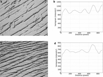
To illustrate the relationship between vario functions and crevasse images, a global vario function (numerically equivalent to the global variogram; see Reference HerzfeldHerzfeld, 2002) is given in Figure 3. The numerical implementation of the vario-function calculation makes use of the organization of pixels and uses several algorithms specially designed to retain spatial information while reducing computation time. In practice, we use residual vario functions, standardized to maximum value of 1. Vario functions are calculated in several directions. The advantage of the vario function is that it is built on increment values, and hence absolute radiometric reference is not needed. In practice, the classification is not affected by the direction or intensity of lighting during image collection. To ascertain that flight direction and camera pointing does not affect the crevasse classification, directional vario functions are calculated. Furthermore, the algorithm is trained to ensure independence from rotation and translation. To identify the neural-net topology of the MPL-BP, pre-training using simplified and simulated crevasse patterns was undertaken. Further detailing of the numerical and computational aspects of the connectionist-geostatistical methods lies beyond the scope of this paper.
Illustration of the relationship between crevasse-pattern images and vario functions. Here the global variogram is shown ((a, c) images; (b, d) variograms). The algorithm for the connectionist classification utilizes discretized four-directional residual vario functions.
6. Classes of Surge Crevasses
The following crevasse types are used as the basis of the classification: (0) undisturbed surface or snow surface, (1) chaos, (2) parallel crevasses, (4) acute-angle bidirectional crevasses, (5) bidirectional crevasses with one dominant direction, (6) square-top blocky crevasses, (7) rhombic crevasses, (8) en-echelon crevasses. Examples of these types as observed during September 2011 are shown in Figure 4. Parallel crevasses (class 2) result from extension and form parallel to the direction of the extensional force. Parallel crevasses can also be caused by compression and then form in the direction normal to the direction of the acting force; however, extension prevails during a surge. Acute-angle bidirectional crevasses (class 4) form when one-directional extension is accompanied by a relatively small amount of shear. Bidirectional crevasses with one dominant direction (class 5) are caused by extensional forces acting in two directions, but with a much stronger force in one direction and a weaker force in the other direction. These usually form in two generations. Square-top blocky crevasses (class 6) form when two-dimensional extension occurs, where forces acting in two directions are equal and the directions of force are normal to each other. Square-top blocky crevasses are common signs of a surge and were observed at the start of the surge in 1993, but also at later stages. Rhombic crevasses (class 7) form under similar conditions to square-top blocky crevasses, but the directions of force are not normal. En-echelon crevasses (class 8) form when a force breaks at preexisting weaknesses and indicate two different deformation events. A first deformation event leads to opening of a crevasse field, then a second, weaker kinematic event affects the crevasse field and causes feathery-appearing small crevasses along the edges of the first generation of crevasses. Depending on the size of the force, the feathery en-echelons may visually dominate the original crevasses. En-echelon crevasse fields are typically observed in Bagley Ice Field and indicate the progression of the kinematic wave associated with the surge into an area that previously has not been affected by the surge. The pre-existing crevasses are often found in extensions of topographic spurs which likely continue under the ice; the subglacial extensions cause crevassing. We call these morphologically induced crevasses. The kinematic force of the surge wave far from its origin near the collapsing reservoir may be too weak to cause crevassing in unbroken ice, but strong enough to cause en-echelon crevasse fields when it reaches an area of morphologically induced crevasses (Reference Herzfeld and MayerHerzfeld and Mayer, 1997). The class ‘chaos’ (class 1) is associated with crevasse fields that have experienced several deformation events that cannot be reconstructed individually any more. Undisturbed surfaces or snow surfaces form the rest class of the crevasse classification. The classes are the same as used in the classification of the 1993–95 surge, except that class 3 (parallel crevasses filled with snow) was not observed and is left out in the neural net. From the input images, all possible rotations are created.
Crevasse types of the Bering Glacier surge in 2011 used in connectionist–geostatistical classification. Images from September 2011.

7. Training and Validation of the Neural Net
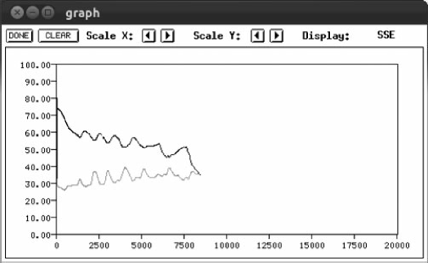
The topology of the neural net is given in Figure 5. The neural net is first trained with simulated images showing simplified crevasse patterns. The learning curve is seen in Figure 6. Class association employs a simple winner-takes-all rule. Once the neural net training is completed, it needs to be validated using data not included in the training runs (Fig. 4).
Neural network used for crevasse classification.

Training curve for neural net (simulated crevasse images). The training set (black line) error (y-axis) decreases as the number of training cycles (x-axis) increases. The validation-set (grey line) error remains fairly constant with continued training. A network is trained when minimal error is reached.
8. Discussion and Outlook
The connectionist–geostatistical method works well to derive deformation types from aerial image data. Because crevasse provinces have sizes on the order of several kilometers and are homogeneous with respect to deformation types, the association of deformation matrices to locations on the glacier is correct, as can be evaluated using visual comparison with overview photographs.
Application of the connectionist–geostatistical method to imagery from flight tracks covering the entire glacier system will allow the creation of a segmentation of the glacier into deformation provinces, at a single point in time. The segmentation can be turned into an automatically derived map of the deformation state at that time point. Time series formed from several such maps will allow mapping of the surge progression.
However, limitations in position accuracy in the current analysis are due to (1) handheld operation of all cameras and (2) lack of recording of aircraft attitude. This complicates automatic processing of images, especially geolocation. In addition, contrary to expectation, time-coincident or near-time satellite imagery was only acquired for a small part (one-sixth) of the Bering–Bagley glacier system (satellite image data acquisition is controlled by an agency that is unrelated to this project, and while data can be acquired after collection, data acquisition strategies cannot currently be changed for science purposes). In aerial observations planned by our group for summer 2012, an integrated system with a nadir-pointing laser and a nadir-pointing camera will be used, together with a GPS system and an inertial measurement unit (IMU) recording aircraft position and attitude. More precisely, laser profilometer and video camera point in a direction normal to the aircraft, which corresponds to nadir for a level plane position. The integrated system will be operated through an opening in the aircraft bottom, which facilitates continuous operation during all flights. Resultant data will allow a significant reduction of the geolocation error in automated processing and hence improve the accuracy of automated segmentation of the glacier into structural provinces.
9. Summary
The objective of this paper is to introduce an automated connectionist–geostatistical classification method as an approach to map deformation stages and surge progression. The approach is demonstrated for the current (2011) surge of the Bering Glacier and Bagley Ice Valley.
The approach employs the concept of a structural province, which is an area that is maximal with respect to homogeneity of deformation, observed as crevassing. Images of crevasses serve as input data for the analysis. In the application to the current surge of the Bering–Bagley glacier system, aerial image data were collected from small aircraft in September 2011 and geolocated approximately using GPS data.
The classification method allows the use of imagery as geophysical data. To this extent, the method utilizes geostatistical vario functions as a means to capture relevant spatial information while reducing data volume, before a neural network is trained and applied for association of crevasse classes or deformation types to output from the vario-function calculation. In this paper, individual images are classified. Application to imagery that covers the entire Bering–Bagley glacier system will allow derivation of a thematic map of the glacier system that shows deformation types, and extension to several time-steps is expected to provide a systematic mapping as well as an objective quantification of surge progression in space and time.
Acknowledgements
This paper is dedicated to the memory of Austin Post who studied Bering Glacier during several of its previous surges and knew more about Alaskan surge glaciers than any other person in glaciological history. The first author was fortunate to share many good field days with Austin during 1993 and 1994 at Bering Glacier. Thanks are due to Bruce Molnia for alerting U.C.H. to the start of the surge in June 2011, to Maciej Stachura for help with field data collection in 2011, to our pilot Terry Kennedy, to Katie and Tom Prijatel of Alaska Wilderness Air, Cordova, to Oliver Zahner for discussion of the 1993–95 classification and to Thomas Trantow for help with figure preparation. Support of the research presented here through the US National Science Foundation’s Arctic Natural Research Program under award ARC-1148800 and Research Experience for Undergraduates (award ARC-1247839) is gratefully acknowledged, the latter especially by the junior co-author, A.W. Support through the University of Colorado Undergraduate Research Opportunity Program is equally appreciated.



