2. Bivariate Gamma Mixture of Experts Model Family for Joint Claim Severity

This section reviews a form of bivariate gamma distributions and their associated bivariate gamma MoE model family, as introduced in Hu et al. (Reference Hu, Murphy and O’Hagan2019). The particular type of the bivariate gamma distributions focused on in the mvClaim package is the one provided by Cheriyan (Reference Cheriyan1941) and Ramabhadran (Reference Ramabhadran1951), and detailed in Mathai & Moschopoulos (Reference Mathai and Moschopoulos1991), which is largely overlooked in the literature so far; to the authors’ knowledge, there is no current implementation of such distributions in R. The bivariate case of the multivariate gamma distribution (BG) is primarily used in the MoE frameworks in mvClaim.

Let $X_1, X_2, X_3$ be independent gamma random variables, where $X_i \sim \mbox{Gamma}(\alpha_i, \beta)$ for $i=1, 2, 3$, with different shape parameters $\alpha_i > 0$ and a common rate parameter $\beta > 0$. Then vector $\textbi{Y}$ is defined as

(1) \begin{equation}\textbi{Y} = \begin{bmatrix} Y_1 \\ \\[-8pt] Y_2 \end{bmatrix} = \begin{bmatrix} X_1+X_3 \\ \\[-8pt] X_2+ X_3 \end{bmatrix} \sim \textrm{BG}(\alpha_1, \alpha_2, \alpha_3, \beta)\end{equation}

It follows that it has density

(2) \begin{align}f_{Y_1, Y_2}(y_1,y_2) = \frac{\beta^{\alpha_1+\alpha_2+\alpha_3}e^{-\beta(y_1+y_2)}}{\Gamma(\alpha_1)\Gamma(\alpha_2)\Gamma(\alpha_3)} \int_{x_3=0}^{\min(y_1, y_2)} e^{\beta x_3} x_3^{\alpha_3 - 1} (y_1 - x_3)^{\alpha_1 -1} (y_2 - x_3)^{\alpha_2 -1} dx_3\end{align}

Since the density is not of analytical form, numerical integration is needed to calculate the density.

Within mvClaim, following the standard notation of functions to compute the probability density function (pdf) and to generate variates from the specified distribution in R, the utility functions are named dbivgamma and rbivgamma, respectively. For example,

The MoE model facilitates modelling, extending the standard mixture models to allow the parameters of the model to depend on concomitant covariates $\textbi{w}_i$, and can be interpreted as model-based clustering with covariates or mixtures of regressions for predictions. Let $\textbi{y}_1, \textbi{y}_2, \ldots, \textbi{y}_n$ be an identical and independently distributed bivariate sample of outcomes from a population. Suppose the population consists of G components. Each component can be modelled by a bivariate gamma distribution $f(\textbi{y}_i|\theta_g)$ with component-specific parameters $\theta_g = \{ \alpha_{1g}, \alpha_{2g}, \alpha_{3g}, \beta_g \}$, for $g=1,\ldots,G$ and $i=1,\ldots,n$. There are also vectors of concomitant covariates $\textbi{w}_1,\textbi{w}_2, \ldots,\textbi{w}_n$ available on which the distribution parameters depend, and which are used to predict future outcome variables. The observed density (conditional on covariates $\textbi{w}_i$) is

(3) \begin{align}p(\textbi{y}_{i}|\textbi{w}_i) &= \sum_{g=1}^{G} \tau_g(\textbi{w}_i) p(y_{1i}, y_{2i}|\theta_g(\textbi{w}_i)) \nonumber\\[3pt] &= \sum_{g=1}^{G} \tau_g(\textbi{w}_{0i}) p(y_{1i}, y_{2i}| \alpha_{1ig}(\textbi{w}_{1i}), \alpha_{2ig}(\textbi{w}_{2i}), \alpha_{3ig}(\textbi{w}_{3i}), \beta_{i}(\textbi{w}_{4i}))\end{align}

where

(4) \begin{align}\log(\alpha_{kig}) &= \boldsymbol{\gamma}_{kg}^{\top} \textbi{w}_{ki}, \ \ \ \text{for} \ \ \ k=1,2,3 \nonumber\\[3pt] \log(\beta_{ig}) \ &= \boldsymbol{\gamma}_{4g}^{\top} \textbi{w}_{4i}\end{align}

and $\tau_g$ is the mixing proportion, i.e. $\sum_{g=1}^{G} \tau_g =1$. Different (subsets of) concomitant covariates $\textbi{w}_{i}$ can go to different parts of the regression models for different parameters since the parameters are independent of each other and hence there exists $\textbi{w}_{0i},\textbi{w}_{1i},\textbi{w}_{2i},\textbi{w}_{3i},\textbi{w}_{4i}$. In the machine learning literature, $\tau_g(\textbi{w}_{0i})$ is called the gating network and $p(y_{1i},y_{2i}|\theta_g(\textbi{w}_i))$ is called the expert network. When the mixing proportion is regressed on covariates, it is typically modelled using a multinomial logistic regression, with $\hat{\tau}_g(\textbi{w}_{0i}) = \frac{\exp(\hat{\boldsymbol{\gamma}}_{0g}^{\top} \textbi{w}_{0i})}{\sum_{g^{\prime}=1}^{G^{\phantom{f}}}\exp(\hat{\boldsymbol{\gamma}}_{0g^{\prime}}^{\top}\textbi{w}_{0i}) }$ (when $G=2$ it becomes a logistic regression). The expert network $p(y_{1i},y_{2i}|\theta_g(\textbi{w}_i))$ is typically modelled via a GLM framework with a log link function. $\boldsymbol{\gamma}_{0g}$, $\boldsymbol{\gamma}_{1g}$, $\boldsymbol{\gamma}_{2g}$, $\boldsymbol{\gamma}_{3g}$, $\boldsymbol{\gamma}_{4g}$ are the regression coefficients for each parameter and component group.

For MoE it is possible that none, some or all model parameters could depend on the covariates; and since all parameters $\alpha_{1g}$, $\alpha_{2g}$, $\alpha_{3g}$, $\beta_g$ are independent of one another, interest lies in allowing more parsimonious parameterisations within the bivariate gamma MoE. Depending on the parameterisation of the framework, its interpretations, and whether one allows covariates to be incorporated in the mixing proportions and/or the bivariate gamma densities of the finite mixture models, a family of models is proposed, including:

1. • Bivariate gamma distribution estimation: implemented via the function BGE.

2. • Bivariate gamma regression: implemented via the function BGR, for EE, EI and IE model types.

3. • Mixture of bivariate gamma clusterings: implemented via the function MBGC, for ^*CC, ^*CI and ^*IC model types.

4. • Mixture of bivariate gamma regressions (i.e. mixture of bivariate gamma clusterings with covariates): implemented via the function MBGR, for ^*VC, ^*VI, ^*VV, ^*VE, ^*CV, ^*IV, ^*EV, ^*EC and ^*CE model types.

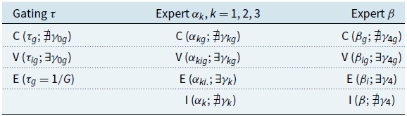
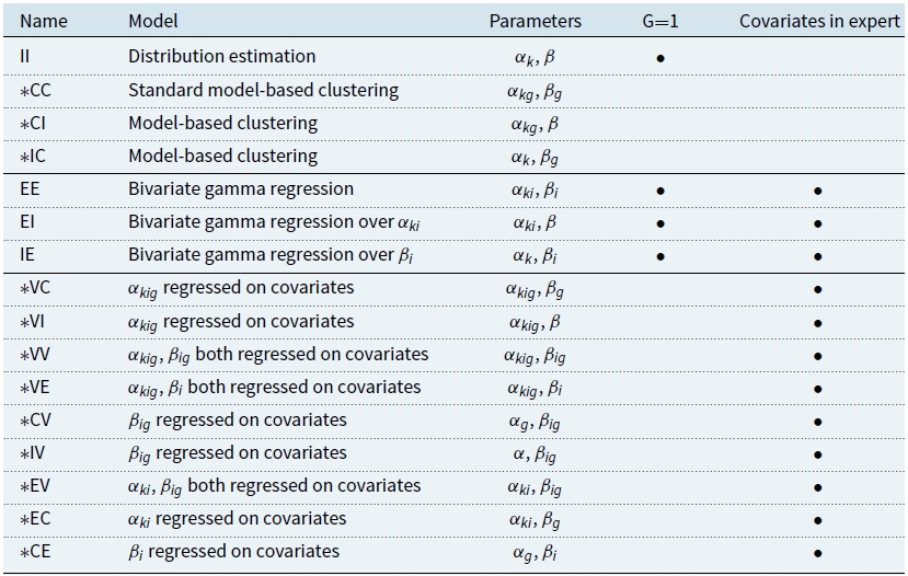
The notation “^*’’ represents the gating network, which can be either E (equal), C (constant) or V (variable); within the expert networks, C represents constant density parameters without covariates, I represents identical density parameters without covariates, V represents variable parameter values depending on covariates and E represents equal parameters depending on covariates. The summaries of the model notation and model types are presented in Tables 1 and 2.

Table 1.

Parsimonious parameterisations of the bivariate gamma MoE models. Each $\boldsymbol{\tau}, \boldsymbol{\alpha}, \boldsymbol{\beta}$ can be modelled via different choices, depending on whether covariates are used in modelling that parameter

Table 2.

Bivariate gamma MoE model family based on parsimonious parameterisation: under each model name “$\ast$’’ represents the gating network, which can be either “C’’ (with covariates), “V’’ (no covariates) or “E’’ (predefined mixing proportion $1/G$). While all models are possible when $G=1$, they are essentially equivalent to one of the four models indicated by “$\bullet$’’. It also indicates which models have covariates in the expert networks. In the table, $k=1,2,3$ for different $\alpha$

2.1 BGE: bivariate gamma distribution estimation

Given there are observations from a bivariate gamma distribution, the distribution parameters can be estimated via:

Estimated parameters:

The summary function shows final estimated parameter values, which are very close to the true values in data simulation.

2.2 MBGC: mixture of bivariate gamma clustering

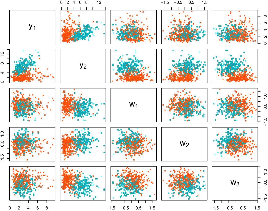
The function MBGC implements model-based clustering with bivariate gamma distributions, allowing covariates to enter gating networks if needed. There are three model types within this bivariate gamma MoE family: ^*CC, ^*CI and ^*IC. The mvClaim package contains several simulated data sets. The detailed simulation process can be found in each data set’s documentation in mvClaim. One such data set is called gatingsim, simulated based on a gating network MoE, i.e. covariates were used only in the gating network to assist with identifying which component the observation was from. The detailed data simulation description can be found in the data set documentation in the package. The pairwise plot of the data are shown in Figure 1, via:

Figure 1

Scatter plot matrix of the simulated data set, coloured by component membership: the teal “$\textcolor{greennew}{\square}$’’ is component 1 and the red “$\textcolor{red}{\times}$’’ is component 2.

Assuming that the data are a mixture of bivariate gamma distributions and there are no covariates in the experts networks, and the expert network is of type CC and the gating network is of type C or E, the mixture model can be fitted via:

Note that fitting G=1 in this case will be equivalent to using the BGE function, and when G=1 in MBGC it is equivalent to setting gating = “C’’ or gating = “E’’. Model types can also be set using modelName = “CI” or modelName = “IC”. For the fitted models c0–c6, the best model according to AIC is c1 with the model summary:

MBGC CCC model with two components:

Gating Network Covariates: None

Estimated expert networks parameters:

Clustering table:

Furthermore, covariates can enter the gating network with, for example, gating = w1+w2+w3. For the artificially simulated data set gatingsim, we know the true data generating process of this data set which can be fitted via:

MBGC VCC model with two components:

Gating Network Covariates: w1 + w2 + w3

Estimated expert networks parameters:

Clustering table:

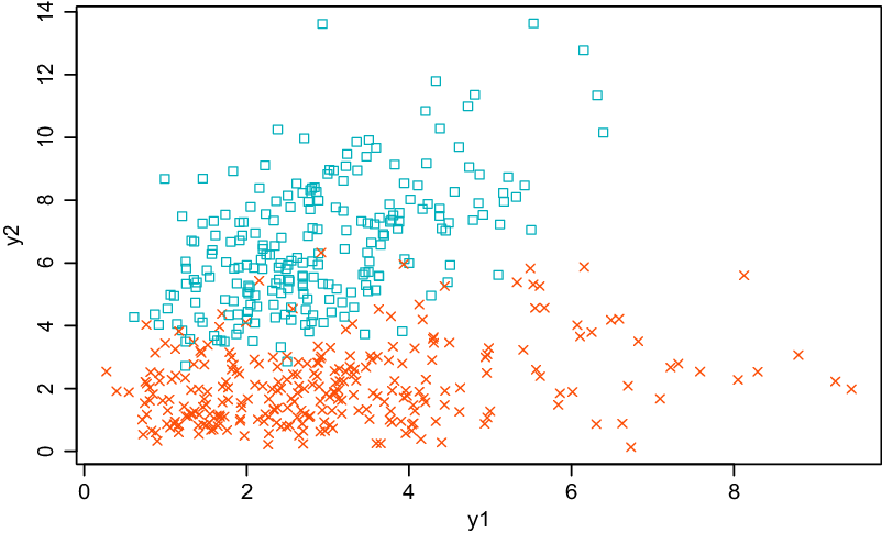
The estimated parameter values are very close to the true data generating process. See the package documentation for gatingsim for the true values. The classification plot is shown in Figure 2, via:

Figure 2

The classification plot of the two components of the c9 model: the teal “$\textcolor{greennew}{\square}$” is component 1 and the red “$\textcolor{red}{\times}$” is component 2.

More details about the data set gatingsim and the analysis can be found in Hu et al. (Reference Hu, Murphy and O’Hagan2019).

2.3 BGR: bivariate gamma regression

Bivariate gamma regression (with no mixtures) can be implemented via the function BGR. The function includes three model types, namely EE, EI and IE, see Table 2. Within the mvClaim package, there is a sample data set that is artificially simulated based on one bivariate gamma regression (with no mixtures) called bgr.sim. The details of how this data set is simulated can be found in the data documentation, via ?bgr.sim, and this data set will be used for illustration of the BGR procedure:

The summary of, for example, model d1 can be extracted as

BGR EE model :

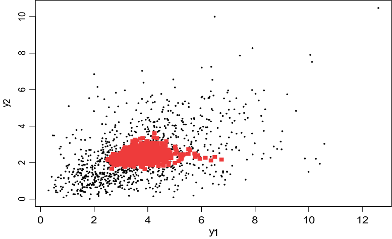
Predictions can be achieved via the predict function, with the plot shown in Figure 3. Clearly the fitted values capture the dependence structure and the overall trend within the data.

Figure 3

The fitted values of the model d1, where the true values are plotted in small black “$\centerdot$’’ and the predictions are plotted in red “$\textcolor{red}{\blacksquare}$’’. Clearly the fitted values are able to capture the dependence structure within the data.

2.4 MBGR: mixture of bivariate gamma regressions

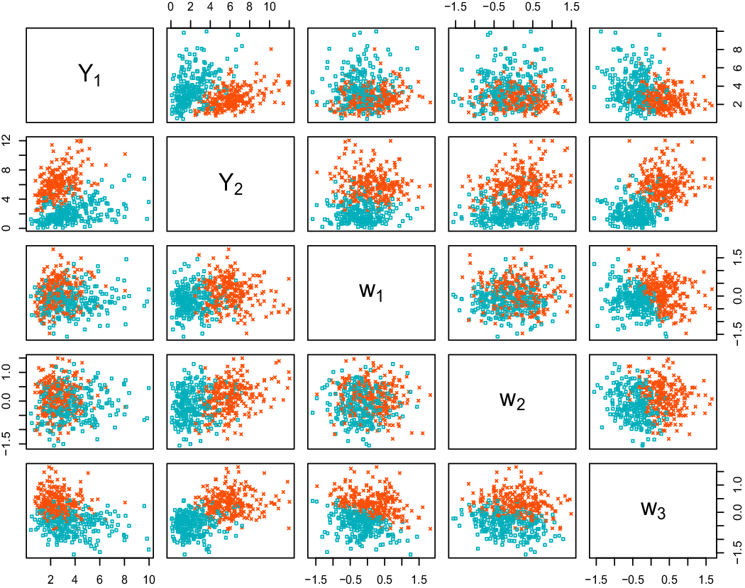
The function MBGR is illustrated using another simulated data set called fullsim as illustrated in Hu et al. (Reference Hu, Murphy and O’Hagan2019), available in the mvClaim package. The data were simulated based on a full MoE model, i.e. with covariates entering both the gating and experts networks. The detailed simulation process can be found in data documentation within the package using ?finsim. The data set is loaded and plotted using the following code, and the pairwise plot of the data are shown in Figure 4:

Figure 4

Scatter plot matrix of the simulated data set, coloured by component membership: the teal “$\textcolor{greennew}{\square}$’’ is component 1 and the red “$\textcolor{red}{\times}$’’ is component 2.

We consider only the cases when covariates are entering the expert networks. In such cases, there are nine different model types: ^*VC, ^*VI, ^*VV, ^*VE, ^*CV, ^*IV, ^*EV, ^*EC, ^*CE. Typically the model selection issue needs to be addressed if the true model is unknown. We recommend stepwise forward selection starting from a null model, i.e. fitting one bivariate gamma distribution without covariates. Then either add one extra component to the current optimal model, or change the model type, or add one covariate to any (combination) of the expert networks of the current model. If $G \geq 2$, covariates should also be added to the gating network. More details can be found in Hu et al. (Reference Hu, Murphy and O’Hagan2019). This will lead to many models to be fitted. The optimal model can be identified using AIC or BIC. Here, since the true model is known, it can be fitted via:

MBGR VVV model with two components:

Clustering table:

The estimated coefficients can be extracted via:

$expert$alpha2

$expert$alpha3

$expert$beta

$gating

which are very close to the true parameter values in the data simulation process.

If focusing only on the clustering result, the classification based on the mixture of bivariate gamma distributions with covariates can be plotted via:

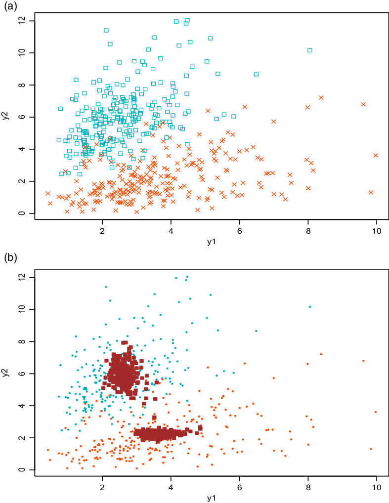
The plot is shown in Figure 5. Furthermore, the plot function also allows the fitted values of the model to be plotted, as shown in Figure 5, via:

Figure 5

The fitted e1 model: (a) shows the classification plot of $\textbi{y}$, where the teal “$\textcolor{greennew}{\square}$’’ is component 1, the red “$\textcolor{red}{\times}$” is component 2; (b) shows the fitted values, where the true values are plotted in small teal and red “$\centerdot$’’ and the predictions are plotted in maroon “’’.

This plot shows that the model is able to capture the two components with roughly two regression lines, following the overall structure of the data.

There is also an accompanying fullsim.test data set available in mvClaim that has been simulated similarly for test data prediction purposes. Based on the fitted model, predictions on the new data can be done via:

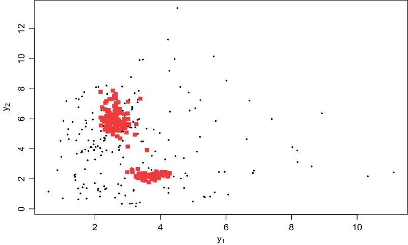
The predictions are plotted in Figure 6. Clearly the out-of-sample predictions identified the dependence structures within two different components. In fact, the predicted values are the means of the predictive distributions and each prediction has a distribution. It can also be shown that these predictions are better than separate univariate GLM modelling. See Hu et al. (Reference Hu, Murphy and O’Hagan2019) for more details.

Figure 6

Predicted values of $\textbi{y}$ for the test data using model e1. The true values are plotted in small black “$\centerdot$’’ and the predictions are plotted in red “$\textcolor{red}{\blacksquare}$’’. Clearly the predicted values identified the dependence structures within different components and can be shown to perform better than those of univariate modelling.

3. Finite Mixture of Copula Regressions

Although it is often preferred to model joint risks using bivariate distributions directly, this can be conceptually challenging due to the complex specification and implementation of such distributions compared to univariate distributions. There is also a limited number of options for such bivariate distributions. When modelling joint insurance claim risks, a copula is another popular option in the literature. The mvClaim package includes implementation of copulas in a MoE framework, namely finite mixtures of copula clusterings and regressions, built on top of the popular copula package on CRAN.

Suppose there are two random variables, $Y_1$ and $Y_2$, with joint distribution function $F(y_1,y_2)$ and two marginal distributions $F_1(y_1)$ and $F_2(y_2)$, respectively. By Sklar’s theorem (Sklar (Reference Sklar1959)) any bivariate CDF can be written in the form

(5) \begin{equation}F(y_1,y_2) = C\left[F_1(y_1),F_2(y_2)\right]\end{equation}

where the function C(u, v) is a copula (Joe, Reference Joe1997; Nelsen, Reference Nelsen2007; Joe, Reference Joe2014). There are various approaches to estimating the parameter $\theta$ of a given parametric copula $C(\theta)$, which also depends on estimation of the marginal distributions. For a review, please refer to Hu & O’Hagan (Reference Hu and O’Hagan2021). When the marginal distributions are estimated parametrically, covariates can be incorporated in the marginals following a GLM framework as extra information, assisting in marginal and further parametric copula estimations. This is sometimes called copula regression (Yan, Reference Yan2007; Masarotto & Varin, Reference Masarotto and Varin2017; Kraemer et al., Reference Kraemer, Brechmann, Silvestrini and Czado2013). Furthermore, copulas can also be mixed to form finite mixtures of copulas for complex and heterogeneous dependence structures, see Kosmidis & Karlis (Reference Kosmidis and Karlis2016) and Arakelian & Karlis (Reference Arakelian and Karlis2014). Therefore, copulas can be estimated via such finite mixtures of copula regressions, following the MoE models construction and inference.

The setup of the copula MoE model is now briefly reviewed, following Hu & O’Hagan (Reference Hu and O’Hagan2021). Suppose there are bivariate identical and independently distributed data $\textbf{\textit{y}}_1, \ldots, \textbf{\textit{y}}_N$ of size N, which consist of G components. There also exist vectors of covariates $\textbf{\textit{x}}_1, \ldots, \textbf{\textit{x}}_N$, based on which let $\textbf{\textit{X}}_j$ be the covariate design matrix for margin j, for $j = 1, 2$; i.e. covariates are not necessarily the same for both marginals. Each component g can be specified by a copula function $C_g$ and two marginal distributions of CDF $F_{jg}$ and PDF $f_{jg}$, for $g = 1, \ldots, G$. Now let $\boldsymbol{\alpha}_g$ be the copula parameter, $\boldsymbol{\beta}_{jg}$ be the regression coefficients of margin j, $\gamma_{jg}$ be any distribution specific parameters of margin j (e.g. shape parameters of gamma distributions), so that each margin follows a specified distribution within a GLM framework such as $\mu_{ji} = \delta^{-1}(\textbf{\textit{x}}_{ijg}^{\top} \boldsymbol{\beta}_{jg})$ where $\delta$ is the link function. Then each component can be regarded as a bivariate distribution (or component-specific copula regression), denoted as $h_g(\textbf{\textit{y}}_i;\ \boldsymbol{\theta}_g)$, where $\boldsymbol{\theta}_g = \left\{\boldsymbol{\alpha}_g, \boldsymbol{\beta}_{jg}, \boldsymbol{\gamma}_{jg} \right\} $. The observed data likelihood of the mixture copula model is

(6) \begin{align}\mathcal{L}(\boldsymbol{\theta}) &= \prod_{i=1}^{N} \sum_{g=1}^{G} \tau_g h_g(\textbf{\textit{y}}_i;\ \boldsymbol{\theta}_g) \nonumber\\&= \prod_{i=1}^{N} \sum_{g=1}^{G} \tau_g c_g\left(F_1(y_{1i};\ \boldsymbol{\beta}_{1g},\boldsymbol{\gamma}_{1g}), F_2(y_{2i};\ \boldsymbol{\beta}_{2g},\boldsymbol{\gamma}_{2g});\ \boldsymbol{\alpha}_g\right) f_1(y_{1i};\ \boldsymbol{\beta}_{1g},\boldsymbol{\gamma}_{1g}) f_2(y_{2i};\ \boldsymbol{\beta}_{2g},\boldsymbol{\gamma}_{2g})\end{align}

where $\tau_g$ is the mixing proportion, i.e. $\sum_{g=1}^{G} \tau_g = 1$ and $c_g$ is the density of a specified copula. This model is estimated via the EM algorithm (Dempster et al., Reference Dempster, Laird and Rubin1977).

The mixtures of copula regressions functions are demonstrated here using a simulated data set called simdat.mcgr. The data were simulated based on a mixture of two copula regressions, i.e. covariates were used to estimate the marginal distributions to assist in the mixture of copulas estimation. Details of the sample data simulation process can be found in the package data documentation and Hu & O’Hagan (Reference Hu and O’Hagan2021). The true data generating process for the data set simdat.mcgr is known, based on which the model can be fitted via:

Mixture of gumbelCopula and frankCopula model, two components:

Clustering table:

The estimated coefficients can be extracted via

R> f1$coefficients

$beta1

$shape1

$beta2

$shape2

$gating

NULL

which are close to the true parameter values in the data simulation process.

If G=1, as an alternative, copula regression with gamma GLMs as marginals (no mixtures) can be fitted via, for example,

gumbelCopula(1.6177) regression:

4. Conclusion and Remarks

This paper illustrates various functionalities of the R package mvClaim targeting joint insurance claims severity modelling, using two approaches: bivariate gamma distributions and bivariate copulas with gamma marginals. By using both methods, not only is the dependence structure taken into account in regression for simultaneously modelling two risks, but different claim patterns can be identified with different dependence structures, targeting the heterogeneity issue.

The package is still undergoing active development and in future further functionality will be added. For example, the current version of the package only focuses on bivariate joint severity modelling, whereas in real-world applications, it may be necessary to consider more risk perils simultaneously. Therefore, higher dimensional cases of the MoE model family using multivariate gamma distributions will form part of the future work. This package does not cover the frequency aspect of joint insurance claims modelling, using bivariate or multivariate Poisson distributions, or copulas targeted for count data. In the literature, there is some existing work in this area and the authors hope to include this in the package over time. Furthermore, this package focuses on joint insurance claims predictions and clustering heterogeneous risks, but does not cover further collective risk analysis using joint cumulative distribution functions, particularly using convolution of bivariate gamma distributions. This will be part of our future work in this area. Finally, to cite the package in publications, please use the citation information given in