



1. Introduction
The dynamics of non-spherical particles in wall-bounded flows underpins a broad range of natural and industrial processes, including pollen dispersion (Sabban & van Hout Reference Sabban and van Hout2011), biomass combustion (Cui & Grace Reference Cui and Grace2007), papermaking (Lundell, Söderberg & Alfredsson Reference Lundell, Söderberg and Alfredsson2011) and targeted drug delivery (Kleinstreuer & Feng Reference Kleinstreuer and Feng2013). Such particle-laden flows represent a central theme in multiphase flow research, posing marked multiscale challenges to the scientific community (Marchioli et al. Reference Marchioli2025). In such settings, predictive models for hydrodynamic forces are essential for Euler–Lagrange point-particle simulations, where the accuracy of the resolved carrier flow directly depends on the force closures employed (Kuerten Reference Kuerten2016; Subramaniam & Balachandar Reference Subramaniam and Balachandar2022).
The theoretical foundation for non-spherical particle motion in viscous flows was laid a century ago by Jeffery (Reference Jeffery1922), who derived the equations governing the rotation of an ellipsoidal particle in Stokes flow. This work was elegantly extended by Brenner (Reference Brenner1963, Reference Brenner1964) to provide analytical expressions for forces on particles of arbitrary shape. These correlations have been widely adopted to study ellipsoidal particle-laden flows in various contexts, e.g. in the numerical investigations of particle transport and orientation dynamics by Marchioli, Fantoni & Soldati (Reference Marchioli, Fantoni and Soldati2010), Zhao & Van Wachem (Reference Zhao and van Wachem2013), Zhao et al. (Reference Zhao, George and van Wachem2015a , Reference Zhao, Challabotla, Andersson and Varianob ) and Zhao & Andersson (Reference Zhao and Andersson2016). While these classical solutions provide a cornerstone for understanding, their strict applicability is limited to inertia-free, unbounded flows.
The introduction of finite inertia and, crucially, a nearby wall, dramatically alters the underlying physics. For spherical particles, the effects of a wall have been systematically mapped, yielding well-established corrections for drag (Brenner Reference Brenner1961; Goldman, Cox & Brenner Reference Goldman, Cox and Brenner1967a ,Reference Goldman, Cox and Brenner b ; Zeng et al. Reference Zeng, Najjar, Balachandar and Fischer2009). For non-spherical particles, however, the problem is intrinsically more complex. The loss of symmetry introduces particle orientation as an additional, dynamically significant variable. Consequently, the drag force depends on the particle Reynolds number, the aspect ratio, the particle orientation and the dimensionless wall distance (Chéron & van Wachem Reference Chéron and van Wachem2024). This multi-parameter dependence, combined with the nonlinear nature of the coupling, renders the development of a general predictive drag model particularly challenging (Bhagat & Goswami Reference Bhagat and Goswami2022), a challenge that is representative of the broader complexities in modelling particle–fluid interactions (Marchioli et al. Reference Marchioli2025).
Over the past decade, significant progress has been made in developing empirical correlations for hydrodynamic forces on non-spherical particles in unbounded flows at finite Reynolds numbers (Chhabra, Agarwal & Sinha Reference Chhabra, Agarwal and Sinha1999; Michaelides & Feng Reference Michaelides and Feng2023). Early contributions by Hölzer & Sommerfeld (Reference Hölzer and Sommerfeld2008) introduced a drag correlation accounting for particle shape, orientation and Reynolds number effects. Subsequent advances in numerical methods enabled more detailed investigations. For example, Zastawny et al. (Reference Zastawny, Mallouppas, Zhao and van Wachem2012) employed direct numerical simulations (DNS) with the immersed boundary method to predict drag across various non-spherical geometries, while Ouchene et al. (Reference Ouchene, Khalij, Tanière and Arcen2015, Reference Ouchene, Khalij, Arcen and Tanière2016) utilised body-fitted meshes to compute drag, lift and torque coefficients for ellipsoidal particles in uniform flow, establishing correlations at moderate Reynolds numbers.
The role of particle orientation was further examined by Sanjeevi & Padding (Reference Sanjeevi and Padding2017) and Sanjeevi, Kuipers & Padding (Reference Sanjeevi, Kuipers and Padding2018), who examined the drag dependence on particle alignment across a broad Reynolds number range, and reported a sinusoidal-like angular dependence persisting even at high Reynolds numbers. More recently, Fröhlich et al. (Reference Fröhlich, Meinke and Schröder2020) employed an adaptive Cartesian cut-cell approach to simulate flow around prolate spheroids, and Sanjeevi, Dietiker & Padding (Reference Sanjeevi, Dietiker and Padding2022) extended this line of work by developing force and torque correlations spanning from the Stokes regime to high Reynolds numbers. A general drag correlation for spherocylinders was proposed by Feng & Michaelides (Reference Feng and Michaelides2023). In addition, Chéron et al. (Reference Chéron, Evrard and van Wachem2024) considered both locally uniform and locally linear shear flows, providing a physically interpretable decomposition of force contributions together with clearly defined regimes of validity. Collectively, these studies have substantially advanced the quantitative understanding of non-spherical particle dynamics in unbounded flows, and the resulting correlations are now widely employed in Euler–Lagrange simulations (Zhong et al. Reference Zhong, Yu, Liu, Tong and Zhang2016). Applications include the fluidisation of non-spherical particles (Atxutegi et al. Reference Atxutegi, Kieckhefen, Pietsch, Aguado, Olazar and Heinrich2021; Mema & Padding Reference Mema and Padding2021) and the transport of non-spherical particles in carrier flows (Hilton & Cleary Reference Hilton and Cleary2011; van Wachem et al. Reference van, Berend, Marian and Mallouppas2015).
Recent studies have begun to examine non-spherical particle configurations in direct contact with walls. Fillingham et al. (Reference Fillingham, Vaddi, Bruning, Israel and Novosselov2021) performed DNS of prolate spheroids resting on a smooth wall in linear shear flow, developing reduced-order models for drag, lift and torque that explicitly account for Reynolds number, aspect ratio and orientation. De Souza et al. (Reference De Souza, Ouchene and Thomas2024) observed a robust sinusoidal-like angular dependence of drag on orientation for oblate spheroids in direct wall contact, suggesting that this scaling may persist under strong confinement. Using the lattice Boltzmann method, Gao et al. (Reference Gao, Hu, Meng, Cui, Mao and Liu2025) investigated wall-attached ellipsoids in shear flow and developed criteria for particle detachment, while Cao et al. (Reference Cao, Li, Liu, Zhang, Tafti, Wang, Yuan and Hu2025) extended the Reynolds number range for oblate ellipsoids and developed further drag correlations. These studies provide valuable data and convenient fitting formulae for particles in direct contact with a wall.
The intermediate regime of finite wall distance, where particles are neither in contact with the wall nor far enough for wall effects to be negligible, has received increasing attention. In the viscous regime, Gavze & Shapiro (Reference Gavze and Shapiro1997) employed a boundary integral method to analyse ellipsoids in shear near a wall, showing that wall-induced drag enhancement diminishes with increasing particle asphericity. Bhagat & Goswami (Reference Bhagat and Goswami2022) examined spheroids near a rough wall, focusing on vertically oriented configurations. More recently, Chéron & van Wachem (Reference Chéron and van Wachem2024) conducted extensive particle-resolved DNS of axisymmetric rod-like particles in wall-bounded linear shear flow, systematically varying wall distance, aspect ratio, orientation and Reynolds number. Based on this database, they derived comprehensive correlations for drag, lift and torque coefficients, valid for particles from direct wall contact to distances outside the boundary layer. This marks a major advance for rod-like particles and is directly applicable in Euler–Lagrange simulations. These works represent a significant step towards quantifying the coupled influence of wall distance, particle orientation and finite Reynolds number on hydrodynamic forces.
Despite these advances, several aspects warrant further investigation. First, most existing studies for finite wall distance focus on rod-like particles with orientation varying in the streamwise–wall-normal plane. For prolate spheroids (a common non-spherical shape in many applications), the full three-dimensional orientation space – characterised by both an azimuthal angle
 $\alpha _H$
and a vertical inclination angle
 $\alpha _V$
(see figure 1) – has not been systematically explored under confinement. Second, while empirical correlations exist for specific parameter ranges, a unified framework that seamlessly connects the wall-attached limit, the finite-distance regime and the unbounded-flow limit while maintaining physical interpretability remains desirable. Such a framework should (i) resolve the three-dimensional orientation dependence, (ii) account for the progressive influence of confinement as the wall is approached, and (iii) remain consistent with established asymptotic limits.
Schematic illustration of the geometrical configuration. The horizontal azimuthal angle
 $\alpha _H$
is measured in the
 $x$
–
 $z$
plane from the streamwise direction, and the vertical inclination angle
 $\alpha _V$
is measured between the major axis and the wall-parallel plane.

Figure 1. Long description
A schematic illustration of the geometrical configuration of non-spherical particles in wall-bounded flows. The diagram shows a particle represented as an ellipsoid positioned above a wall. The particle has a major axis and a minor axis. The horizontal azimuthal angle is measured in the plane from the streamwise direction, and the vertical inclination angle is measured between the major axis and the wall-parallel plane. The diagram includes labels for the angles, the radius of the particle, and the distance from the wall. Arrows indicate the directions of the angles and the flow. The coordinate system is shown with axes labeled x, y, and z.
The present study addresses these aspects through a combination of theoretical analysis and numerical simulations. We develop a hierarchical drag model that is systematically constructed from the fundamental Stokes-flow solution for ellipsoids. The framework progressively incorporates finite-inertia effects and wall confinement through physically motivated correction functions, and finally reconstructs the full angular dependence from a minimal set of reference orientations. The formulation is constructed to ensure asymptotic consistency, recovering both the exact unbounded Stokes behaviour and established wall-contact limits. To validate the theoretical model, we perform a comprehensive DNS investigation of prolate spheroids with aspect ratio
 $\lambda = 2$
in wall-bounded shear flow, spanning a broad range of Reynolds numbers (
 $0.5 \leqslant \textit{Re} \leqslant 115$
), normalised wall distances from near contact (
 $G/D_e = 0.1$
) to the nearly unbounded regime (
 $G/D_e = 1.5$
), and the complete orientation space defined by
 $(\alpha _H,\alpha _V)$
.
The remainder of the paper is organised as follows. Section 2 introduces the drag model framework, beginning with the unbounded-flow formulation and then incorporating wall corrections, orientation scaling and the overall reconstruction strategy. Section 3 describes the numerical methodology, including the governing equations, computational set-up, parameter space and convergence validation. Section 4 presents the simulation results, covering validation in unbounded flow, wall correction mechanisms, orientation scaling under confinement, and overall model performance. Finally, § 5 summarises the key findings and outlines avenues for future research.
2. Drag model framework
We consider a prolate spheroid fixed in a linear shear flow,
 $U_{x}=K_x y$
, close to an infinite planar wall, as depicted in figure 1. The minimum wall–particle distance is denoted by
 $G$
. The spheroid is defined by its semi-major and semi-minor axes,
 $b$
and
 $a$
, respectively, giving an aspect ratio
 $\lambda = b/a$
. The particle is held at prescribed orientation angles
 $\alpha _H$
and
 $\alpha _V$
.
The development of a drag model for this configuration proceeds from fundamental physical principles to increasingly complex configurations. We begin with the well-established behaviour in unbounded flows, subsequently introduce wall-confinement effects, and finally establish orientation scaling relationships to complete the predictive framework.
2.1. Unbounded-flow drag formulation
The foundation of our drag model begins with the exact Stokes-flow solution for prolate spheroids in unbounded flow, which provides the theoretical basis for shape and orientation effects. To ensure consistency across all formulations, we first establish the unified definitions of key parameters.
The drag coefficient, which serves as the primary metric throughout this study, is defined as
 \begin{equation} C_d = \frac {F_d}{\dfrac {1}{2} \rho U_{\textit{ref}}^2 A_{\textit{ref}}}, \end{equation}
where
 $F_d$
denotes the streamwise drag force acting on the spheroid,
 $U_{\textit{ref}}$
is the characteristic reference velocity, and
 $A_{\textit{ref}} = \pi D_e^2 / 4$
is the projected area of the volume-equivalent sphere of diameter
 $D_e$
. In particular, for the considered prolate spheroid,
 $D_e = 2(a^2 b)^{1/3}$
, where
 $b$
and
 $a$
represent the semi-major and semi-minor axes, respectively. For stationary particles in shear flow, the reference velocity is defined as the undisturbed free-stream velocity that would exist at the particle centroid position in the absence of the particle:
 \begin{equation} U_{\textit{ref}} = K_x y_c, \end{equation}
where
 $K_x$
is the constant shear rate, and
 $y_c$
is the wall-normal position of the particle centroid. This definition follows the established approach for characterising shear flow conditions around stationary particles (e.g. Fillingham et al. Reference Fillingham, Vaddi, Bruning, Israel and Novosselov2021).
To characterise the flow conditions, we define two key Reynolds numbers based on consistent velocity scaling. The particle Reynolds number is defined as
 \begin{equation} \textit{Re} = \frac {\rho U_{\textit{ref}} D_e}{\mu } = \frac {\rho K_x y_c D_e}{\mu }, \end{equation}
where
 $\rho$
is the fluid density, and
 $\mu$
is the dynamic viscosity. In our wall-bounded shear flow configuration, we additionally define the shear Reynolds number as
 \begin{equation} \textit{Re}_s = \frac {\rho K_x D_e^2}{\mu }. \end{equation}
The geometric relationship between these two Reynolds numbers is obtained by expressing the centroid height
 $y_c$
in terms of the wall distance
 $G$
and the particle geometry. As illustrated in figure 1, the centroid height is
 $y_c = G + R$
, where
 $R$
is the vertical distance from the particle centroid to the surface point nearest to the wall. For a prolate spheroid with aspect ratio
 $\lambda$
, this distance depends on the vertical inclination angle
 $\alpha _V$
and is given by the ellipsoid geometry,
 $R = (D_e/2\lambda ^{1/3}) \sqrt {1 + (\lambda ^2 - 1)\sin ^2 \alpha _V}$
. Substituting
 $y_c = G + R$
into the definition of
 $\textit{Re}$
and using the expression for
 $\textit{Re}_s$
yields the relation
 \begin{equation} \textit{Re} = \frac {\rho K_x D_e^2}{\mu }\frac {G+R}{D_e}=\left ( \frac {G}{D_e} + \frac {\sqrt {1 + (\lambda ^2 - 1)\sin ^2 \alpha _V}}{2 \lambda ^{1/3}} \right ) \textit{Re}_s, \end{equation}
which establishes the fundamental connection between the particle-based Reynolds number
 $\textit{Re}$
and the flow-based shear Reynolds number
 $\textit{Re}_s$
. This relation explicitly accounts for the effects of wall proximity (
 $G/D_e$
), particle aspect ratio (
 $\lambda$
) and vertical orientation (
 $\alpha _V$
) on the relationship between these two Reynolds numbers.
In unbounded flow, the rotational symmetry of the system implies that the particle orientation can be fully described by a single angle. For a prolate spheroid in a uniform incoming stream, this angle is defined as that between the major axis and the flow direction, denoted by
 $\alpha \in [0, \pi /2]$
. In the Stokes regime, the drag coefficient for a prolate spheroid can be expressed as the product of the Stokes drag for a sphere and an orientation-dependent correction factor:
 \begin{equation} C_{d,\textit{Stokes}}^{\textit{ellipsoid}} = \frac {24}{\textit{Re}} \times K(\alpha ), \end{equation}
where
 $K(\alpha )$
is derived from the exact Stokes-flow solution for an ellipsoid, and accounts for the change in drag due to the non-spherical geometry at a given orientation angle
 $\alpha$
.
For the two principal orientations with respect to the flow, the correction factors depend solely on the aspect ratio
 $\lambda$
and are given by Happel & Brenner (Reference Happel and Brenner1983). Let
 $K_{\parallel }$
denote the factor when the major axis is aligned with the flow (
 $\alpha =0$
), and let
 $K_{\perp }$
denote the factor when the major axis is perpendicular to the flow (
 $\alpha =\pi /2$
):
 \begin{equation} K_{\parallel } = K(0) = \frac {8}{3\lambda ^{1/3}} \left [ \frac {2\lambda ^2 - 1}{(\lambda ^2 - 1)^{3/2}} \ln \frac {\lambda + \sqrt {\lambda ^2 - 1}}{\lambda - \sqrt {\lambda ^2 - 1}} - \frac {2\lambda }{\lambda ^2 - 1} \right ]^{-1}, \end{equation}
 \begin{equation} K_{\perp } = K(\pi /2) =\frac {8}{3\lambda ^{1/3}} \left [ \frac {\lambda }{\lambda ^2 - 1} + \frac {2\lambda ^2 - 3}{(\lambda ^2 - 1)^{3/2}} \ln (\lambda + \sqrt {\lambda ^2 - 1}) \right ]^{-1}. \end{equation}
To extend this Stokes-flow solution to finite Reynolds numbers, we introduce Reynolds number correction factors that capture the inertial effects. The complete expressions for the unbounded-flow drag coefficients become
 \begin{equation} C_{d, \parallel }^{\textit{uni}} = \frac {24}{\textit{Re}} \times K_{\parallel } \times f_{\parallel }(\textit{Re}), \end{equation}
 \begin{equation} C_{d,\perp }^{\textit{uni}} = \frac {24}{\textit{Re}} \times K_{\perp } \times f_{\perp }(\textit{Re}), \end{equation}
where
 $C_{d, \parallel }^{\textit{uni}}$
is the drag coefficient for flow parallel to the major axis at finite Reynolds numbers,
 $C_{d,\perp }^{\textit{uni}}$
is the drag coefficient for flow perpendicular to the major axis at finite Reynolds numbers, and
 $f_{\parallel }(\textit{Re})$
and
 $f_{\perp }(\textit{Re})$
are the Reynolds number correction factors for parallel and perpendicular orientations, respectively.
The functional form of the Reynolds number correction factors is motivated by the Schiller–Naumann correlation for spheres (Schiller Reference Schiller1933), but with orientation-dependent coefficients:
 \begin{equation} f_{\parallel }(\textit{Re}) = 1 + a_1\, \textit{Re}^{b_1}, \end{equation}
 \begin{equation} f_{\perp }(\textit{Re}) = 1 + a_2\, \textit{Re}^{b_2}, \end{equation}
where
 $a_1$
,
 $b_1$
,
 $a_2$
and
 $b_2$
are empirical coefficients determined through fitting to DNS data by Fröhlich et al. (Reference Fröhlich, Meinke and Schröder2020) and Sanjeevi et al. (Reference Sanjeevi, Dietiker and Padding2022). This formulation ensures the correct asymptotic behaviour: as
 $\textit{Re} \rightarrow 0$
,
 $f_{\parallel }(\textit{Re}) \rightarrow 1$
and
 $f_{\perp }(\textit{Re}) \rightarrow 1$
, recovering the exact Stokes-flow solution.
Overall, the proposed formulation extends the analytical Stokes solution to moderate Reynolds numbers while preserving its inherent dependence on shape and orientation. The introduction of orientation-specific inertial correction factors provides a smooth transition from viscous-dominated to inertia-influenced regimes, yielding an accurate and robust drag representation for ellipsoidal particles in unbounded flow.
2.2. Wall correction formulation
Building upon the unbounded-flow behaviour, we now introduce wall-confinement effects through a physically motivated model that accounts for the complex hydrodynamic interactions between ellipsoidal particles and nearby boundaries. Our fundamental assumption, analogous to established approaches for spherical particles, is that the wall-bounded drag coefficient
 $C_d(\alpha _H,\alpha _V)$
can be expressed as the product of the corresponding unbounded-flow drag and an orientation-dependent wall correction factor
 $K_{wi}$
:
 \begin{equation} C_d(0, 0) = C_{d,\parallel }^{\textit{uni}}\times K_{w1} , \end{equation}
 \begin{equation} C_d(\pi /2, 0) = C_{d,\perp }^{\textit{uni}}\times K_{w2}, \end{equation}
 \begin{equation} C_d(0, \pi /2) = C_{d,\perp }^{\textit{uni}} \times K_{w3}, \end{equation}
where
 $C_d(0, 0)$
denotes the drag coefficient for a particle aligned with the flow direction and parallel to the wall,
 $C_d(\pi /2, 0)$
represents the drag coefficient for horizontal transverse orientation, and
 $C_d(0, \pi /2)$
corresponds to vertical transverse orientation. The terms
 $C_{d,\parallel }^{\textit{uni}}$
and
 $C_{d,\perp }^{\textit{uni}}$
refer to the unbounded-flow drag coefficients for parallel and perpendicular orientations, respectively, as defined in (2.9) and (2.10).
The wall correction factors
 $K_{wi}$
(with
 $i = 1,2,3$
corresponding to the three reference orientations, i.e.
 $(0,0)$
,
 $(\pi /2,0)$
and
 $(0,\pi /2)$
) quantify the drag enhancement due to wall confinement and are expected to depend on both the dimensionless wall distance
 $G/D_e$
and flow inertia characterised by the shear Reynolds number
 $\textit{Re}_s$
. Based on our analysis of the DNS data for these reference orientations, we propose the functional form
 \begin{equation} K_{wi} = 1 + c_i\, \textit{Re}_s^{-d_i}\, \mathrm{e}^{-e_i G/D_e}, \end{equation}
where
 $c_i$
,
 $d_i$
and
 $e_i$
are empirical coefficients specific to each reference orientation and thus do not vary with
 $\alpha _H$
or
 $\alpha _V$
. This formulation ensures asymptotic behaviour: as
 $G/D_e \rightarrow \infty$
,
 $K_{wi} \rightarrow 1$
, recovering the unbounded-flow limit. The exponential dependence on
 $G/D_e$
captures the spatial decay of confinement influence with increasing wall distance, while the power-law dependence on
 $\textit{Re}_s$
represents the progressive attenuation of wall effects with increasing flow inertia, with the exponent
 $d_i$
quantifying the rate of this inertial attenuation.
The physical interpretation of these correction factors relates to the disruption of flow patterns near the wall. As particles approach the boundary, several effects contribute to drag amplification, e.g. constriction of flow passages leading to accelerated fluid velocities and increased shear rates, and disruption of symmetric wake structures of unbounded flows. The orientation dependence emerges from how each configuration modifies the geometry of the narrowest flow passage and consequently alters the local velocity gradients and pressure distributions.
The empirical coefficients are determined through systematic fitting to our comprehensive DNS database, with the specific values for each reference orientation presented in § 4.2. This approach captures the progressive increase in drag resistance as particles approach the wall while maintaining the essential coupling between orientation effects and confinement strength.
2.3. Orientation scaling relationships
With the drag coefficients at the three reference orientations established via the wall correction formulation, we now proceed to develop scaling relationships capable of predicting the drag over the full orientation space. The starting point is the analytical Stokes-flow solution for an ellipsoid in unbounded flow, where the linearity of the governing equations leads to an exact functional dependence on orientation.
For a prolate spheroid in Stokes flow, the hydrodynamic resistance is described by the tensor
 \begin{equation} \boldsymbol{\varXi } = \xi _{\parallel } (\hat{\boldsymbol {n}} \otimes \hat{\boldsymbol {n}}) + \xi _{\perp } (\boldsymbol{I} - \hat{\boldsymbol {n}} \otimes \hat{\boldsymbol {n}}), \end{equation}
where
 $\xi _{\parallel }$
and
 $\xi _{\perp }$
are the resistance coefficients for motion parallel and perpendicular to the main symmetry axis
 $\hat{\boldsymbol {n}}$
, respectively. This structure implies that the drag coefficient in unbounded flow varies with the angle
 $\alpha$
(between
 $\hat{\boldsymbol {n}}$
and the flow) as
 $C_d(\alpha ) = C_d(0) + [C_d(\pi /2)-C_d(0)] \sin ^2\alpha$
(Happel & Brenner Reference Happel and Brenner1983).
When a nearby wall is present, the flow field is no longer symmetric under arbitrary rotations of the particle. However, rotations of the particle about the wall-normal axis preserve the minimum gap
 $G$
. This remaining symmetry suggests that at a fixed vertical inclination
 $\alpha _V$
, the dependence on the horizontal azimuthal angle
 $\alpha _H$
may retain a form analogous to the unbounded case. We therefore propose the following scaling for the horizontal orientation dependence:
 \begin{equation} C_d(\alpha _H,\alpha _V) = C_d(0,\alpha _V) + \left [C_d(\pi /2,\alpha _V) - C_d(0,\alpha _V)\right ]\sin ^2\alpha _H, \end{equation}
where
 $C_d(\alpha _H,\alpha _V)$
is the drag coefficient at the horizontal azimuthal angle
 $\alpha _H$
and vertical inclination angle
 $\alpha _V$
, while
 $C_d(0,\alpha _V)$
and
 $C_d(\pi /2,\alpha _V)$
denote the reference drag coefficients for streamwise-aligned and horizontally transverse orientations, respectively, at fixed vertical inclination
 $\alpha _V$
.
In contrast to horizontal rotations, variations in the vertical inclination angle
 $\alpha _V$
significantly modify the geometric confinement experienced by the particle. As
 $\alpha _V$
varies, the effective projection of the spheroid towards the wall changes, thereby altering the local distortion of the near-wall velocity field. The orientation is thus directly coupled to the confinement effect. Unlike the horizontal azimuthal dependence, which largely preserves the tensorial structure characteristic of unbounded flow, the vertical dependence is altered by wall proximity and cannot be described by a simple
 $\sin ^2$
scaling. To account for this behaviour, we introduce the following expression for the vertical dependence:
 \begin{equation} C_d(\alpha _H,\alpha _V) = C_d(\alpha _H,0) + \left [ C_d(\alpha _H,\pi /2) - C_d(\alpha _H,0) \right ] \sin ^{2 - \gamma }(\alpha _V), \end{equation}
where
 $C_d(\alpha _H,0)$
and
 $C_d(\alpha _H,\pi /2)$
denote the reference drag coefficients corresponding to the wall-parallel and vertically transverse configurations, respectively, at fixed azimuthal orientation
 $\alpha _H$
. The exponent correction
 $\gamma$
characterises the modification of the vertical scaling induced by confinement. Analysis of the full DNS database indicates that
 $\gamma$
depends primarily on the dimensionless wall distance
 $G/D_e$
, while its variation with
 $\alpha _H$
and
 $\textit{Re}_s$
is comparatively weak. Accordingly, we model
 $\gamma$
as a function of
 $G/D_e$
alone:
 \begin{equation} \gamma = m\mathrm{e}^{-nG/D_e}, \end{equation}
where
 $m$
and
 $n$
are empirical coefficients determined from a global fit to the DNS dataset and are independent of
 $\alpha _H$
and
 $\textit{Re}_s$
. The exponential form in (2.20) provides a compact representation of the confinement-induced modulation of the vertical scaling, affecting only the interpolation between the two reference orientations without altering the reference drag coefficients themselves. Moreover, its impact becomes negligible at sufficiently large wall distances, where the classical
 $\sin ^2\alpha _V$
scaling is recovered.
The complete framework achieves remarkable efficiency by requiring characterisation of only three reference orientations –
 $C_d(0, 0)$
,
 $C_d(\pi /2, 0)$
and
 $C_d(0, \pi /2)$
– yet successfully predicts drag coefficients across the entire orientation space through the coupled application of (2.18) and (2.19). These two scaling relations are mutually consistent: applying (2.18) followed by (2.19) yields the same drag coefficient as the reverse order, regardless of the chosen interpolation path. This property, which follows from the algebraic structure of the model and the fact that both relations share the same reference values, ensures a unique and self-consistent prediction for any orientation
 $(\alpha _H,\alpha _V)$
. This approach maintains asymptotic consistency with established unbounded-flow theory while efficiently capturing the complex nonlinear interactions between particle orientation and wall confinement.
The distinct scaling behaviours for horizontal and vertical rotations arise from their fundamentally different geometric interactions with wall confinement. Horizontal rotations (varying
 $\alpha _H$
) occur about the wall-normal axis, preserving the minimum wall gap
 $G$
. Consequently, the drag variation with
 $\alpha _H$
stems primarily from changes in the effective frontal area, retaining a quadratic angular dependence analogous to that in unbounded flow. In contrast, vertical rotations (varying
 $\alpha _V$
) directly alter the projection of the particle’s major axis along the wall-normal direction, thereby significantly modifying the geometric blocking effect experienced by the particle. This reorientation introduces nonlinear distortion into the dependence of drag on
 $\alpha _V$
. Under strong confinement (small
 $G/D_e$
), this blocking effect, amplified by geometric constraints, becomes particularly pronounced, leading to nonlinear saturation in the vertical inclination dependence.
2.4. Model reconstruction strategy
The complete modelling framework follows a hierarchical three-step procedure that progresses from baseline unbounded-flow behaviour to near-wall configurations. This structure allows the drag in wall-bounded shear flow to be constructed systematically from physically interpretable components. The formulation separates the contributions of particle shape, orientation and confinement, while retaining their essential coupling through the correction terms introduced at each stage.
Step 1: unbounded-flow reference. Establish the baseline behaviour by computing orientation-dependent drag coefficients in unbounded flow using (2.7)–(2.12). This foundation leverages the exact Stokes solution for prolate ellipsoids, providing the theoretical basis for shape and orientation effects, while the Reynolds number corrections capture inertial modifications through empirically validated scaling.
Step 2: wall-confinement correction. Incorporate wall effects through orientation-dependent correction factors applied to the three reference configurations using (2.13)–(2.16). The functional form captures the progressive attenuation of wall effects with increasing distance and Reynolds number while ensuring proper asymptotic behaviour.
Step 3: orientation reconstruction. Reconstruct drag at arbitrary orientations through coupled scaling relationships using (2.18)–(2.20).
This hierarchical formulation preserves asymptotic consistency with established unbounded-flow theory while incorporating near-wall effects through physically motivated correction terms. In the low-Reynolds-number limit and at large wall distances, the model recovers the corresponding Stokes-flow and unbounded-flow behaviour. The separation of baseline drag, inertial modification and confinement correction enables a transparent interpretation of how each physical mechanism contributes to the total drag. The parametrisation relies on three reference orientations, from which the drag over the full orientation space is reconstructed through interpolation governed by the proposed scaling relations. The exponent correction
 $\gamma$
adjusts the vertical inclination dependence according to the degree of confinement, thereby accounting for the progressive modification of geometric blocking effects as the wall distance decreases.
The empirical coefficients (
 $a_1$
,
 $b_1$
,
 $a_2$
,
 $b_2$
,
 $c_i$
,
 $d_i$
,
 $e_i$
with
 $i=1,2,3$
,
 $m$
,
 $n$
) are reported in § 4, where the predictive performance of the model is assessed quantitatively against the DNS data across the investigated parameter space. The resulting formulation provides a compact representation of orientation- and confinement-dependent drag suitable for implementation in Euler–Lagrange simulations, while avoiding unnecessary parameter proliferation.
3. Numerical method
This section presents the numerical framework for investigating hydrodynamic forces on a prolate spheroid in wall-bounded shear flow. The governing equations and numerical schemes are first introduced, followed by details of the computational set-up and parameter space. Systematic grid- and domain-independence tests are then performed to ensure numerical accuracy and reliability, and the numerical set-up is subsequently validated against established reference data.
3.1. Governing equations and numerical methodology
For the steady-state simulations considered in this work, the flow is governed by the steady incompressible Navier–Stokes equations. In a three-dimensional Cartesian coordinate system, they are expressed as
 \begin{equation} \frac {\partial U_i}{\partial x_i} = 0, \end{equation}
 \begin{equation} U_{\!j} \frac {\partial U_i}{\partial x_{\!j}} = -\frac {1}{\rho } \frac {\partial P}{\partial x_i} + \nu \frac {\partial ^2 U_i}{\partial x_{\!j}^2}, \end{equation}
where
 $x_i = (x, y, z)$
denote the Cartesian coordinates,
 $U_i$
are the corresponding velocity components,
 $P$
is the pressure,
 $\rho$
is the fluid density, and
 $\nu$
is the kinematic viscosity.
The adoption of steady-state simulations is well established in the literature for studying particle drag forces at low to moderate Reynolds numbers, as demonstrated in previous investigations of non-spherical particle hydrodynamics (Ouchene et al. Reference Ouchene, Khalij, Tanière and Arcen2015; Fillingham et al. Reference Fillingham, Vaddi, Bruning, Israel and Novosselov2021). This approach is justified by the Reynolds number range investigated in the present study (
 $0.5 \leqslant \textit{Re} \leqslant 115$
), where flow separation remains limited, and the wake structure maintains stability for prolate spheroids across all orientations considered. The critical Reynolds number for transition to unsteady flow depends significantly on particle shape and orientation; while flow past a sphere becomes unsteady at
 $\textit{Re} \approx 270{-}280$
(Johnson & Patel Reference Johnson and Patel1999), ellipsoidal particles with aspect ratio
 $\lambda = 2$
maintain steady flow up to
 $\textit{Re} \approx 250$
for both aligned and perpendicular orientations (Richter & Nikrityuk Reference Richter and Nikrityuk2012). Given that our maximum Reynolds number (
 $\textit{Re} = 115$
) falls well below these critical values, steady-state simulations provide an accurate and computationally efficient approach for drag prediction.
To further verify the validity of the steady-state assumption, time-accurate simulations were performed for selected representative cases (including
 $\textit{Re}_s = 50$
,
 $G/D_e = 0.1$
and
 $1.5$
,
 $(\alpha _H,\alpha _V)=(0,\pi /2)$
), integrated over
 $t = 200 D_e / U_{\textit{ref}}$
(Chéron & van Wachem Reference Chéron and van Wachem2024). The time-averaged drag coefficients from these transient simulations differed from the steady-state results by less than
 $1\,\%$
, and the instantaneous flow fields showed no periodic or chaotic variations (not shown for brevity). These tests, together with literature critical Reynolds numbers, confirm that the steady-state solutions faithfully represent the mean flow behaviour within the present parameter range. This finding aligns with the observations of Ouchene et al. (Reference Ouchene, Khalij, Tanière and Arcen2015), who similarly reported minimal differences between steady and transient drag predictions for ellipsoidal particles in the low to moderate Reynolds number regime.
The convective terms were discretised using a second-order upwind scheme (Gauss linearUpwind), while the viscous terms were approximated with a second-order central-differencing scheme (Gauss linear). Under-relaxation was applied to ensure numerical stability during the iterative process. Convergence was deemed achieved when the normalised residuals of all governing equations fell below
 $10^{-8}$
.
3.2. Numerical set-up and parameter space
The computational framework employed in this study is designed to systematically investigate the hydrodynamic forces on prolate spheroids in wall-bounded shear flows. As illustrated in figure 2, a rectangular domain accommodates a prolate spheroid with aspect ratio
 $\lambda = b/a = 2$
, where
 $b$
and
 $a$
represent the semi-major and semi-minor axes, respectively. The coordinate system is established with the origin at the projection of the spheroid’s centroid onto the bottom wall. The
 $x$
,
 $y$
and
 $z$
axes align with the streamwise, wall-normal and spanwise directions, respectively, following established conventions for wall-bounded particle flows (Fillingham et al. Reference Fillingham, Vaddi, Bruning, Israel and Novosselov2021; Chéron & van Wachem Reference Chéron and van Wachem2024). The minimum gap distance
 $G$
between the spheroid surface and the wall is systematically varied to study confinement effects.
(a) Schematic of the computational domain and boundary conditions for a prolate spheroid in wall-bounded shear flow. (b) Computational mesh in the vertical plane through the particle centre (
 $x$
–
 $y$
plane), showing the body-fitted conformal grid and local refinement near the particle surface and within the gap region. A close-up view of the mesh around the particle is provided in the inset.

The particle orientation is parametrised by two angles: the horizontal azimuthal angle
 $\alpha _H$
, measured in the
 $x$
–
 $z$
plane from the streamwise direction, and the vertical inclination angle
 $\alpha _V$
, measured between the major axis and the wall-parallel plane (with
 $\alpha _V = 0$
for wall-parallel, and
 $\alpha _V = \pi /2$
for wall-normal orientation). The computational domain extends over
 $-15D_e \leqslant x \leqslant 45D_e$
,
 $0 \leqslant y \leqslant 20D_e$
and
 $-10D_e \leqslant z \leqslant 10D_e$
, providing sufficient streamwise length for wake development, and adequate spanwise width to minimise lateral boundary effects. Domain sensitivity analyses confirmed that this configuration yields boundary-independent results.
Boundary conditions are carefully prescribed to accurately capture the physical phenomena while minimising artificial constraints. A linear shear profile
 $U_x(y) = K_x y$
is imposed at the inlet, where
 $K_x = \mathrm{d}U_x/\mathrm{d}y$
is the constant shear rate. No-slip conditions are enforced at the bottom wall and spheroid surface, while free-slip conditions at the lateral boundaries prevent unrealistic flow constriction. The outlet employs a zero-gradient Neumann condition for velocity with fixed reference pressure, ensuring smooth flow exit without spurious reflections.
To characterise the coupled effects of flow inertia, particle orientation and wall confinement, an extensive parameter space was explored through 400 DNS, as summarised in table 1. The shear Reynolds number
 $\textit{Re}_s$
ranges from 1 to 50, encompassing viscous-dominated to moderately inertial regimes. The orientation angles
 $\alpha _H$
and
 $\alpha _V$
are systematically varied from 0 to
 $\pi /2$
to ensure full coverage of the orientation space. The dimensionless wall distance
 $G/D_e$
spans 0.1–1.5, thereby capturing configurations from strong confinement to conditions approaching unbounded flow.
Parameter space considered in this study, consisting of 400 DNS that span the shear Reynolds number, horizontal and vertical orientation angles (in radians), and dimensionless wall distance.

Table 1. Long description
The table lists the parameters and their values used in the study. The parameters include the shear Reynolds number, horizontal orientation angle, vertical orientation angle, and dimensionless wall distance. The shear Reynolds number ranges from 1 to 50. The horizontal orientation angle varies from 0 to pi/2 radians. The vertical orientation angle also varies from 0 to pi/2 radians. The dimensionless wall distance spans from 0.1 to 1.5.
This designed numerical set-up and parameter space enable a comprehensive analysis of ellipsoidal particle dynamics across a wide range of flow conditions relevant to practical applications, and in particular, can be used to investigate the performance of the drag model introduced in § 2.
3.3. Numerical convergence and validation
Before proceeding to the validation, we conduct a systematic examination of numerical convergence with respect to grid resolution and domain size. These investigations were performed for shear Reynolds numbers
 $\textit{Re}_s = 1$
, 10 and 50 at representative orientation
 $\alpha _H = \alpha _V = \pi /3$
with dimensionless wall distance
 $G/D_e = 0.1$
. All simulations are performed using a body-fitted, conformal multi-block structured grid generated around the prolate spheroid. The mesh is constructed using an O-grid topology to ensure high orthogonality and smooth cell-size transitions, particularly in the near-wall region and within the narrow gap between the particle and the wall. Special attention is paid to resolving the boundary layers on both the spheroid surface and the bottom wall, with grid stretching applied in the wall-normal direction to cluster cells near the no-slip boundaries. Figure 2(b) illustrates the grid distribution in the symmetry plane for the most challenging case
 $G/D_e=0.1$
, showing the conformal nature of the mesh around the particle, and the progressive refinement towards the wall and the gap region.
The grid independence study compared two mesh resolutions within the same computational domain of dimensions
 $(15, 45, 20, 20)D_e$
in the
 $(x_{\textit{up}}, x_{\textit{down}}, y, z)$
directions. The standard mesh employed a minimum normalised spacing
 $\varDelta _{\textit{min}}/D_e = 0.03$
, corresponding to approximately
 $3.6\times 10^6$
cells, while the fine mesh used
 $\varDelta _{\textit{min}}/D_e = 0.02$
with approximately
 $1.0\times 10^7$
cells. As summarised in table 2, the drag coefficient
 $C_d$
exhibits remarkable consistency between the two mesh resolutions across all Reynolds numbers. The relative error, calculated as
 $\Delta C_d = \left | (C_d^{\textit{standard}} - C_d^{\textit{fine}})/C_d^{\textit{fine}} \right | \times 100\,\%$
, remains below 0.05 % for all cases, with maximum deviation only 0.047 % at
 $\textit{Re}_s=1$
. This exceptional agreement demonstrates that the numerical solution has achieved grid convergence, and the standard mesh provides sufficient spatial resolution to capture the flow physics accurately.
Grid independence study for the drag coefficient
 $C_d$
at
 $\alpha _H = \alpha _V = \pi /3$
and
 $G/D_e = 0.1$
. The relative error
 $\Delta C_d$
is calculated as
 $| (C_d^{\textit{standard}} - C_d^{\textit{fine}})/C_d^{\textit{fine}} | \times 100\,\%$
.

Table 2. Long description
The table presents a grid independence study for the drag coefficient at different Reynolds numbers. It compares two mesh resolutions within the same computational domain. The table has six rows and six columns. Column headers are Mesh, Re, Domain size, Δmin/D, Cd, and ΔCd (percent). Row 1: Mesh, Standard; Re, 1; Domain size, (15, 45, 20, 20); Δmin/D, 0.03; Cd, 50.6775; ΔCd (percent), 0.047. Row 2: Mesh, Fine; Re, 1; Domain size, (15, 45, 20, 20); Δmin/D, 0.02; Cd, 50.6535; ΔCd (percent), —. Row 3: Mesh, Standard; Re, 10; Domain size, (15, 45, 20, 20); Δmin/D, 0.03; Cd, 7.3380; ΔCd (percent), 0.046. Row 4: Mesh, Fine; Re, 10; Domain size, (15, 45, 20, 20); Δmin/D, 0.02; Cd, 7.3414; ΔCd (percent), —. Row 5: Mesh, Standard; Re, 50; Domain size, (15, 45, 20, 20); Δmin/D, 0.03; Cd, 2.7556; ΔCd (percent), 0.029. Row 6: Mesh, Fine; Re, 50; Domain size, (15, 45, 20, 20); Δmin/D, 0.02; Cd, 2.7564; ΔCd (percent), —.
To further assess the dependence of near-wall flow structures on the resolution at very small wall distances, we compare the local flow fields obtained with the standard and fine meshes for the most critical case
 $G/D_e = 0.1$
and
 $\textit{Re}_s = 1$
, where viscous effects are strongest and the flow is most sensitive to grid resolution. Figure 3 compares the normalised streamwise wall shear stress along the particle surface for the same configuration. The two meshes yield virtually indistinguishable wall shear stress distributions, with differences in the peak value remaining below 0.49 %. These observations confirm that the adopted grid resolution is sufficient to resolve the key near-wall flow features even at the smallest gap distance considered. The numerical results are therefore essentially grid-independent with respect to both integrated forces and local flow quantities.
Comparison of the normalised streamwise wall shear stress
 $C_{f,x} = \tau _{w,x} / (({1}/{2})\rho U_c^2)$
on the particle surface for the case
 $G/D_e = 0.1$
,
 $\textit{Re}_s = 1$
,
 $(\alpha _H,\alpha _V)=(\pi /3,\pi /3)$
, obtained with the standard mesh (
 $\varDelta _{\min }/D_e = 0.03$
) and the fine mesh (
 $\varDelta _{\min }/D_e = 0.02$
): (a) windward side, (b) leeward side.

The domain size independence was investigated separately by comparing results obtained with the fine mesh and a large domain mesh, both employing the same minimum grid spacing
 $\varDelta _{\textit{min}}/D_e = 0.02$
to isolate boundary effects from grid resolution effects. The large domain extended the computational boundaries to
 $(20, 60, 30, 30)D_e$
in the
 $(x_{\textit{up}}, x_{\textit{down}}, y, z)$
directions, containing approximately
 $1.2\times 10^7$
cells – a threefold increase in domain volume compared to the standard configuration. As presented in table 3, the deviations in
 $C_d$
between the fine and large domain configurations show a clear Reynolds number dependence. The maximum relative error 1.12 % occurs at the lowest Reynolds number (
 $\textit{Re}_s=1$
), where viscous effects dominate and extend farther into the domain. This error diminishes significantly to 0.43 % at
 $\textit{Re}_s=10$
, and further reduces to 0.09 % at
 $\textit{Re}_s=50$
, indicating that boundary effects become less pronounced at higher Reynolds numbers. Based on these results, the standard mesh with domain size
 $(15, 45, 20, 20)D_e$
is adopted for all subsequent simulations, providing an optimal balance between numerical accuracy and computational efficiency.
Domain size independence study for the drag coefficient
 $C_d$
at
 $\alpha _H = \alpha _V = \pi /3$
and
 $G/D_e = 0.1$
. Both meshes have minimum grid spacing
 $\varDelta _{min}/D_e=0.02$
. The relative error
 $\Delta C_d$
is calculated as
 $| (C_d^{\textit{fine}} - C_d^{\textit{large domain}})/C_d^{\textit{large domain}} | \times 100\,\%$
.

Table 3. Long description
The table presents a comparison of drag coefficients for different mesh sizes and domain sizes at various Reynolds numbers. It has six rows and six columns. The columns are labeled Mesh, Re, Domain size, Δmin/Dc, Cd, and ΔCd (percent). The rows are labeled as follows: Fine, Large domain, Fine, Large domain, Fine, Large domain. The values in the rows are: Row 1: Fine, 1, (15, 45, 20, 20), 0.02, 50.6535, 1.12; Row 2: Large domain, 1, (20, 60, 30, 30), 0.02, 50.0919, —; Row 3: Fine, 10, (15, 45, 20, 20), 0.02, 7.3414, 0.43; Row 4: Large domain, 10, (20, 60, 30, 30), 0.02, 7.3097, —; Row 5: Fine, 50, (15, 45, 20, 20), 0.02, 2.7564, 0.09; Row 6: Large domain, 50, (20, 60, 30, 30), 0.02, 2.7540, —.
Following the convergence, the numerical methodology is further validated against the DNS data of Fillingham et al. (Reference Fillingham, Vaddi, Bruning, Israel and Novosselov2021) for a wall-attached prolate spheroid with the same aspect ratio
 $\lambda = 2$
in wall-bounded shear flow, focusing on the case with
 $\alpha _V = 0$
and varying horizontal azimuthal angle
 $\alpha _H \in [0, \pi /2]$
. As illustrated in figure 4, the present DNS results for the drag coefficient
 $C_d$
agree with the reference data across the Reynolds number range
 $\textit{Re} \in [1, 70]$
, with maximum deviations consistently below 2 %. Beyond quantitative agreement, the data reveal a clear physical trend:
 $C_d$
decreases monotonically with increasing
 $\textit{Re}$
for all azimuthal orientations considered, reflecting the weakening influence of viscous effects at higher Reynolds numbers – consistent with the scaling arguments outlined in § 2. These observations validate the accuracy of the present simulations, and establish confidence in the numerical set-up for the subsequent parametric study.
Comparison of drag coefficient
 $C_d$
as a function of Reynolds number
 $\textit{Re}$
for a wall-attached prolate spheroid (
 $\lambda = 2$
,
 $\alpha _V = 0$
) in wall-bounded shear flow. Present DNS results (circles) are validated against the reference data from Fillingham et al. (Reference Fillingham, Vaddi, Bruning, Israel and Novosselov2021) (triangles). Different colours correspond to varying horizontal azimuthal angles
 $\alpha _H$
: blue for
 $0$
, red for
 $\pi /6$
, green for
 $\pi /4$
, purple for
 $\pi /3$
, and black for
 $\pi /2$
.

4. Results and discussion
4.1. Unbounded-flow validation and baseline behaviour
We first consider a prolate spheroid in an unbounded uniform flow. The accuracy of the baseline formulation for this configuration is evaluated against high-fidelity DNS datasets, establishing its reliability before wall-confinement effects are introduced. Figure 5 compares the present correlations (2.9)–(2.10) with DNS results for an isolated prolate spheroid from Fröhlich et al. (Reference Fröhlich, Meinke and Schröder2020) and Sanjeevi et al. (Reference Sanjeevi, Dietiker and Padding2022). The empirical coefficients
 $a_1 = 0.1625$
,
 $b_1 = 0.6076$
,
 $a_2 = 0.1633$
and
 $b_2 = 0.7200$
are obtained through a least squares fit to the datasets of Fröhlich et al. (Reference Fröhlich, Meinke and Schröder2020) and Sanjeevi et al. (Reference Sanjeevi, Dietiker and Padding2022). Over the Reynolds number range
 $1 \leqslant \textit{Re} \leqslant 100$
, the present formulation shows close agreement with both reference datasets for streamwise-aligned and transverse orientations. To quantify the model accuracy, the mean relative error (MRE) is defined as
 \begin{equation} \mathrm{MRE} = \frac {1}{N} \sum _{k=1}^{N} \left | \frac {C_d^{\textit{DNS}}(k) - C_d^{\textit{model}}(k)}{C_d^{\textit{DNS}}(k)} \right |\!, \end{equation}
where
 $N$
denotes the total number of data points included in the comparison. The median relative error (MedRE) is defined as the median of the same absolute relative deviations. For the unbounded-flow validation against the DNS datasets of Fröhlich et al. (Reference Fröhlich, Meinke and Schröder2020) and Sanjeevi et al. (Reference Sanjeevi, Dietiker and Padding2022), both MRE and MedRE are below
 $2\,\%$
, demonstrating that the baseline formulation accurately captures the drag of isolated prolate spheroids in unbounded flow.
Validation of the unbounded-flow drag formulation for prolate ellipsoids of aspect ratio
 $\lambda = 2$
. Comparison of the empirical fits from (2.9) and (2.10) (red solid line) with DNS data (symbols) from Fröhlich et al. (Reference Fröhlich, Meinke and Schröder2020) and Sanjeevi et al. (Reference Sanjeevi, Dietiker and Padding2022) at orientations: (a)
 $\alpha =0$
and (b)
 $\alpha = \pi /2$
. The DNS data for axisymmetric rod-like particles in unbounded flow from Chéron et al. (Reference Chéron, Evrard and van Wachem2024) are also included for comparison.

The model reproduces the characteristic Reynolds-number dependence observed in DNS. At low to moderate
 $\textit{Re}$
, the drag coefficients decrease rapidly, reflecting the transition from viscous-dominated Stokes flow to regimes in which inertial effects begin to reduce viscous resistance. The formulation captures this curvature for both
 $\alpha =0$
and
 $\alpha =\pi /2$
, demonstrating that the combination of Stokes-based shape factors and inertial correction laws accurately represents the underlying physics. For
 $\textit{Re} \gtrsim 20$
, the decay in drag becomes more gradual as inertial contributions become increasingly balanced by pressure forces. Throughout the range, the transverse configuration maintains a higher drag than the streamwise configuration owing to its larger projected area and enhanced wake formation, a trend faithfully captured by the model. For completeness, the drag coefficients for a rod-like particle with aspect ratio
 $\lambda =2.5$
in unbounded flow (from Chéron et al. Reference Chéron, Evrard and van Wachem2024) are also shown in figure 5. The trends are similar to those of the prolate spheroids (
 $\lambda =2$
), with minor quantitative differences attributable to the different shape and aspect ratio.
A principal strength of the present formulation is its grounding in the Oberbeck solution for Stokes flow around prolate spheroids (Oberbeck Reference Oberbeck1876; Happel & Brenner Reference Happel and Brenner1983). The analytical correction factors
 $K_{\parallel }$
and
 $K_{\perp }$
ensure exact recovery of the Stokes-limit behaviour as
 $\textit{Re} \to 0$
. This analytical structure provides a continuous representation of inertial effects, and naturally extends to incorporate wall corrections while preserving the correct unbounded-flow limit.
The orientation dependence encoded in the analytical correction factors captures the essential anisotropy of prolate spheroids. For the two reference orientations considered here – streamwise (
 $\alpha = 0$
) and transverse (
 $\alpha = \pi /2$
) – the relation
 $K_{\parallel } \lt 1 \lt K_{\perp }$
reflects the reduced drag in streamwise alignment, where the tapered geometry delays separation, and the enhanced drag in the transverse configuration, where the larger projected area and stronger pressure drag contribution dominate. The distinct Reynolds number exponents,
 $b_1 = 0.6076$
(parallel) and
 $b_2 = 0.7200$
(perpendicular), further highlight the differing inertial sensitivities of these limiting orientations. The larger exponent for the transverse case signifies stronger inertial amplification, consistent with flow over bluff projections. These scalings emerge naturally from the formulation, reinforcing its physical fidelity and robustness.
4.2. Wall correction mechanisms and parametrisation
The quantitative influence of wall proximity on particle drag is systematically characterised in figure 6, which presents the wall correction factors
 $K_{wi}$
defined in (2.16) for the three reference orientations: streamwise-aligned
 $(0,0)$
, transverse-horizontal
 $(\pi /2,0)$
, and transverse-vertical
 $(0,\pi /2)$
. Within the parameter range studied, the results show that
 $K_{wi} \gt 1$
for all configurations, and that
 $K_{wi}$
decreases monotonically with increasing
 $G/D_e$
; this trend is consistent across the investigated Reynolds numbers. This enhancement is most pronounced at small distances (
 $G/D_e \lesssim 0.3$
).
Wall correction factors
 $K_{wi}$
as functions of dimensionless wall distance
 $G/D_e$
for the three reference orientations: (a) streamwise-aligned
 $(0,0)$
, (b) transverse-horizontal
 $(\pi /2,0)$
, and (c) transverse-vertical
 $(0,\pi /2)$
. Solid lines represent the model predictions from (2.16); symbols denote DNS data. The DNS data denoted by the star symbols (five-pointed stars and six-pointed stars) for the rod-like particle for the streamwise-aligned configuration from Chéron & van Wachem (Reference Chéron, Evrard and van Wachem2024) are also included for comparison.

Despite this universal monotonic decay behaviour, both the magnitude and spatial decay characteristics of
 $K_{wi}$
exhibit marked orientation dependence. The transverse-horizontal configuration
 $(\pi /2,0)$
displays the strongest confinement response, with
 $K_{w2}$
exhibiting the largest amplitude variation across the
 $G/D_e$
range. This heightened sensitivity stems from the maximal flow blockage presented to the wall in this orientation, where the particle’s major axis lies perpendicular to the flow direction while being parallel to the wall, creating the largest effective obstruction to the near-wall flow. In contrast, the transverse-vertical orientation
 $(0,\pi /2)$
shows the weakest confinement response, as the particle’s major axis aligns with the wall-normal direction, minimising the flow constriction in the gap region. The streamwise-aligned configuration
 $(0,0)$
exhibits intermediate behaviour, with the slender geometry progressively intruding into the high-shear region of the near-wall layer as the gap narrows. For further comparison, we have also included the wall correction data for rod-like particles from Chéron & van Wachem (Reference Chéron and van Wachem2024) for the streamwise-aligned configuration (figure 6
a). The drag enhancement with decreasing wall distance shows consistent trends for both shapes; at
 $\textit{Re}=1$
, the rod-like correction factor is slightly higher, reflecting the influence of particle shape.
Reynolds number effects systematically modulate the wall correction in a secondary but consistent manner. Across all orientations, the correction factors follow a well-defined ordering at small wall distances:
 $K_{wi}(\textit{Re}_s=1) \gt K_{wi}(\textit{Re}_s=10) \gt K_{wi}(\textit{Re}_s=50)$
. This trend reflects the growing influence of fluid inertia at higher
 $\textit{Re}_s$
, which mitigates the pronounced drag amplification – dominated by enhanced viscous stresses in the thin gap region – observed under low-Reynolds-number conditions. As
 $G/D_e$
increases, this Reynolds number dependence progressively weakens, and all curves asymptotically approach the unbounded-flow limit of
 $K_{wi} \to 1$
as wall effects diminish.
These observed orientation-specific and Reynolds-number-dependent behaviours are captured by the parametric model in (2.16), with optimally fitted coefficients provided in table 4. The extracted coefficients elucidate the physical trends observed in figure 6. The amplitude coefficients
 $c_i$
reflect the intrinsic sensitivity to wall proximity, with the transverse-horizontal configuration exhibiting the largest value (
 $c_2 = 0.8709$
), more than twice that of the transverse-vertical orientation (
 $c_3 = 0.4043$
). This hierarchy aligns with the degree of flow blockage, confirming that orientations with larger projected areas normal to the flow experience stronger wall-induced drag enhancement.
Empirical coefficients for the wall correction factors
 $K_{wi}$
defined in (2.16).

Table 4. Long description
A table with three rows and four columns. The columns are labeled ‘Reference orientation (rad)’, ‘c_i’, ‘d_i’, and ‘e_i’. The rows are labeled with different reference orientations and their corresponding coefficients. Row 1: Reference orientation (0, 0), c_i 0.6256, d_i 0.09271, e_i 1.8581. Row 2: Reference orientation (π/2, 0), c_i 0.8709, d_i 0.08796, e_i 2.0223. Row 3: Reference orientation (0, π/2), c_i 0.4043, d_i 0.06329, e_i 1.4004.
The Reynolds number exponents
 $d_i$
are uniformly small (
 $d_i \approx 0.06$
–
 $0.09$
), confirming that inertial effects introduce only minor adjustments to the predominantly viscous near-wall dynamics. By contrast, the gap-dependence exponents
 $e_i$
reveal clear orientation-dependent variations. The transverse-horizontal configuration
 $(\pi /2,0)$
shows the largest value (
 $e_2 = 2.0223$
), indicating a rapid decay of wall influence as confinement weakens, consistent with its strong blockage when close to the wall. The streamwise-aligned case
 $(0,0)$
exhibits a moderately fast decay (
 $e_1 = 1.8581$
). The transverse-vertical configuration
 $(0,\pi /2)$
yields the smallest exponent (
 $e_3 = 1.4004$
), reflecting the most persistent wall effects, consistent with its wall-normal alignment.
The proposed wall correction model provides excellent predictive performance, with the MRE remaining below 2 % across all configurations examined. The particularly high accuracy for the transverse-vertical orientations – where the MRE remains at 1.15 % – demonstrates that the model faithfully reproduces the DNS trends. This parametrisation offers a robust foundation for the drag-prediction framework developed in this study.
To provide more physical insight into the underlying mechanisms for the wall-induced drag enhancement, figure 7 depict the streamwise velocity contours and in-plane streamlines for three representative orientations at the smallest wall distance considered,
 $G/D_e=0.1$
, with
 $\textit{Re}_s=10$
. Although the imposed linear shear profile is identical, the near-wall flow topology and wake structure are strongly modified by particle orientation, revealing distinct drag-enhancement mechanisms.
Streamwise velocity contours and streamlines at
 $G/D_e = 0.1$
and
 $\textit{Re}_s = 10$
for the three orientations (a,d) streamwise-aligned
 $(0, 0)$
; (b,e) transverse-horizontal
 $(\pi /2, 0)$
; and (c, f) transverse-vertical
 $(0, \pi /2)$
, for (a–c)
 $x$
–
 $y$
plane, (d–f)
 $x$
–
 $z$
plane. All planes are taken through the geometric centre of the ellipsoid.

Figure 7. Long description
Panel A: A contour plot showing streamwise velocity around a streamwise-aligned ellipsoid in the plane. The x-axis is labeled x/D_e and the y-axis is labeled y/D_e. The color gradient indicates velocity magnitude, with arrows showing streamlines. Panel B: A contour plot showing streamwise velocity around a transverse-horizontal ellipsoid in the plane. The x-axis is labeled x/D_e and the y-axis is labeled y/D_e. The color gradient indicates velocity magnitude, with arrows showing streamlines. Panel C: A contour plot showing streamwise velocity around a transverse-vertical ellipsoid in the plane. The x-axis is labeled x/D_e and the y-axis is labeled y/D_e. The color gradient indicates velocity magnitude, with arrows showing streamlines. Panel D: A contour plot showing streamwise velocity around a streamwise-aligned ellipsoid in the plane. The x-axis is labeled x/D_e and the y-axis is labeled z/D_e. The color gradient indicates velocity magnitude, with arrows showing streamlines. Panel E: A contour plot showing streamwise velocity around a transverse-horizontal ellipsoid in the plane. The x-axis is labeled x/D_e and the y-axis is labeled z/D_e. The color gradient indicates velocity magnitude, with arrows showing streamlines. Panel F: A contour plot showing streamwise velocity around a transverse-vertical ellipsoid in the plane. The x-axis is labeled x/D_e and the y-axis is labeled z/D_e. The color gradient indicates velocity magnitude, with arrows showing streamlines.
For the streamwise-aligned configuration
 $(0,0)$
, the particle’s slender geometry aligns with the flow, minimising frontal blockage. As shown in figure 7(a), the imposed shear creates a strong asymmetry in the incoming momentum: the upper portion of the particle interacts with higher-momentum fluid, while the lower surface is embedded in a low-speed near-wall region. The narrow gap between the particle and the wall is a defining feature. Streamlines in this gap are strongly compressed and nearly parallel to the wall, indicating intense viscous shearing. Because both the wall and particle surfaces satisfy no-slip conditions, the streamwise velocity within the gap is significantly suppressed, forming an extended low-velocity region beneath the particle. The closely spaced streamlines confirm that viscous shear amplification within the gap is the dominant confinement effect. Above the particle, the higher-momentum fluid is smoothly deflected upwards without abrupt separation, and no jet-like acceleration is observed. The overall flow remains attached, with drag enhancement arising primarily from near-wall momentum suppression rather than large-scale separation.
In the transverse-horizontal configuration
 $(\pi /2,0)$
, the particle presents its maximum frontal area to the flow, intensifying the blockage effect. As shown in figure 7(b), the near-wall fluid undergoes substantial deceleration as it is forced around the particle, creating a pronounced momentum deficit in the lower half of the wake. A key feature is the formation of a small recirculation region on the bottom wall, located immediately downstream of the gap between the particle and the wall. This structure originates not from the particle’s own wake, but from local separation of the wall boundary layer induced by the adverse pressure gradient in the recovery region. The physical mechanism is as follows. As the flow recovers downstream, a positive streamwise pressure gradient is established due to pressure recovery. The near-wall fluid, already weakened by both the background shear and the particle-induced deceleration, lacks sufficient momentum to overcome this adverse gradient, leading to local boundary-layer separation. The recirculation region is confined between distinct separation and reattachment points along the wall. Notably, this separation, which is absent in the other two orientations, explains why this configuration exhibits the maximum drag enhancement and the strongest sensitivity to wall distance under strong confinement (see figure 6). This configuration demonstrates that in addition to viscous gap effects, wall-induced flow separation can contribute to drag enhancement at sufficiently small wall distances.
When the spheroid is vertically inclined to
 $(0,\pi /2)$
, the near-wall flow topology is fundamentally altered. As shown in figure 7(c), the lower surface forms a wedge-shaped gap with the wall, leading to pronounced streamline compression within the minimum-clearance region. Unlike the transverse-horizontal case, however, no wall-attached recirculation bubble is observed downstream. The narrowing of the gap induces local flow acceleration as fluid is squeezed between the particle and the wall. This confinement-driven acceleration is evident from the locally steep velocity gradients and the dense streamline pattern beneath the particle. The mechanism is primarily geometric, arising from continuity constraints rather than inertial jet formation. Downstream of the particle, the wake remains attached to the wall, with the velocity deficit redistributed upwards – reflecting the upward displacement of the frontal stagnation region caused by the vertical inclination. Consequently, the near-wall momentum deficit is less severe than in the transverse-horizontal configuration. The drag modification in this orientation arises from geometric reshaping of the confinement gap and pressure redistribution, rather than from enhanced blockage or wall-induced separation.
The
 $x$
–
 $z$
planes (figures 7
d–f) provide further insight into the lateral flow structures. For the streamwise-aligned configuration (figure 7
d), the wake is narrow and remains fully attached. In contrast, the transverse-horizontal case (figure 7
e) displays a broad spanwise wake, consistent with the wall-attached recirculation region observed in the
 $x$
–
 $y$
plane (figure 7
b). For the transverse-vertical orientation (figure 7
f), the wake is notably more slender in the spanwise direction than in figure 7(e). This narrow wake structure effectively reduces the lateral pressure gradient and suppresses flow detachment, explaining why no recirculation bubble forms in the corresponding
 $x$
–
 $y$
plane (figure 7
c). Ultimately, this confined and elongated wake promotes attached flow, contributing to the lower drag observed for this orientation.
Overall, the three reference orientations reveal qualitatively distinct flow features under strong confinement. The streamwise-aligned case is dominated by viscous shear amplification within the narrow gap, with the flow remaining attached throughout. The transverse-horizontal case exhibits both gap-induced shear enhancement and a downstream wall-attached recirculation bubble caused by adverse pressure gradient. The transverse-vertical case features local flow acceleration within the wedge-shaped gap, and upward redistribution of the wake. Despite these differences, all three configurations share a common feature: the near-wall momentum deficit is significantly amplified compared to unbounded flow, and the flow remains steady and laminar across the parameter range studied. These flow-field observations provide a physical basis for the wall correction factors introduced in § 2.2, and confirm that the dominant drag-enhancement mechanism under strong confinement arises from intensified viscous shear and altered pressure distribution within the confined gap, rather than from large-scale inertial wake effects.
4.3. Orientation scaling under confinement
4.3.1. Azimuthal angle dependence
We first examine the hypothesised
 $\sin ^2\alpha _H$
dependence (2.18) using DNS over a broad range of confinement conditions. Figure 8 shows the normalised drag coefficient as a function of azimuthal angle
 $\alpha _H$
for various wall distances
 $G/D_e$
and shear Reynolds numbers
 $\textit{Re}_s$
. The DNS results (symbols) collapse closely onto the
 $\sin ^2\alpha _H$
curves (solid lines) with MRE below
 $1.49\,\%$
, confirming that the quadratic angular dependence remains preserved under confinement.
Normalised drag coefficient as a function of azimuthal angle
 $\alpha _H$
for different wall distances
 $G/D_e$
and shear Reynolds numbers
 $\textit{Re}_s$
: (a)
 $\alpha _V = 0$
, (b)
 $\alpha _V = \pi /4$
, (c)
 $\alpha _V = \pi /3$
. The normalised drag is defined as
 $(C_d - C_{d,\alpha _H=0})/(C_{d,\alpha _H=\pi /2} - C_{d,\alpha _H=0})$
. Solid lines denote the
 $\sin ^2\alpha _H$
scaling; symbols denote DNS data.

The persistence of this scaling is striking given the strong influence of wall proximity on the absolute drag magnitude (§ 4.2). While confinement substantially modifies the baseline resistance, the relative dependence on azimuthal orientation retains its
 $\sin ^2$
functional form. This observation extends classical results for unbounded flows (Happel & Brenner Reference Happel and Brenner1983; Sanjeevi & Padding Reference Sanjeevi and Padding2017) to wall-bounded configurations, suggesting that for horizontal rotations, the dominant symmetry underlying the drag response is only weakly affected by the presence of a nearby wall.
At finite Reynolds numbers (
 $\textit{Re}_s = 10$
and
 $50$
), inertial effects lead to quantitative changes in the drag magnitude; nevertheless, the
 $\sin ^2 \alpha _H$
dependence continues to describe the DNS data with good accuracy. No systematic deviations indicative of higher-order angular harmonics are observed. The consistency of this behaviour across different vertical inclination angles further underscores the robustness of the
 $\sin ^2 \alpha _H$
scaling.
From a practical standpoint, the verified
 $\sin ^2 \alpha _H$
dependence implies that the azimuthal variation of the drag can be reconstructed from the two limiting orientations (
 $\alpha _H = 0$
and
 $\alpha _H = \pi /2$
). In this sense, the orientation dependence does not require independent characterisation over the full range of
 $\alpha _H$
. This observation can reduce the computational or experimental effort associated with mapping orientation-dependent drag, which is particularly relevant for Euler–Lagrange simulations of particle-laden flows.
4.3.2. Inclination angle dependence
The dependence of drag on the vertical inclination angle
 $\alpha _V$
is strongly modified by wall confinement. Because the minimum distance
 $G$
is fixed, varying
 $\alpha _V$
changes the projection of the particle’s major axis normal to the wall and thus alters the geometric blocking experienced by the near-wall shear flow. Unlike horizontal rotations – which mainly vary the frontal area normal to the flow and preserve a quadratic
 $\sin ^2$
scaling – changes in
 $\alpha _V$
directly redistribute the near-wall flow field, coupling geometry to local flow distortion. Even at constant
 $G$
, increasing
 $\alpha _V$
modifies streamline compression within the gap and reshapes the three-dimensional pressure distribution around the particle. These mechanisms, rather than a simple change in projected frontal area, break the classical
 $\sin ^2$
scaling valid in unbounded flow, and introduce the nonlinear angular dependence observed under confinement.
To represent this departure from quadratic scaling, the model in (2.19) incorporates a confinement-dependent exponent correction
 $\gamma (G/D_e)$
, defined in (2.20). Fitting this relation to our DNS dataset yields coefficients
 $m=1.335$
and
 $n=0.960$
, determined across all orientations rather than being configuration-specific. The parameter
 $\gamma$
quantifies the deviation from the unbounded
 $\sin ^2\alpha _V$
scaling. At small wall distance (
 $G/D_e=0.1$
),
 $\gamma \approx 1.2$
, corresponding to a markedly subquadratic dependence on
 $\sin \alpha _V$
. As the wall distance increases (
 $G/D_e \gtrsim 1$
), the exponent correction
 $\gamma$
progressively decreases towards zero. In this limit, the functional form of the vertical orientation scaling approaches the classical
 $\sin ^2\alpha _V$
dependence associated with unbounded flow. However, at large wall distances, the drag coefficients
 $C_d(\alpha _H,0)$
and
 $C_d(\alpha _H,\pi /2)$
also become increasingly similar. When these two limits nearly coincide, the interpolation between them yields only a weak dependence on
 $\alpha _V$
, regardless of the specific exponent. The exponential form in (2.20) therefore parametrises the dominant confinement-induced modulation of the angular scaling, while preserving the correct asymptotic behaviour in the unbounded-flow limit.
The modelling of the vertical inclination
 $\alpha _V$
can be compared with the results of Chéron & van Wachem (Reference Chéron and van Wachem2024). The observed departure from quadratic scaling is qualitatively consistent with the deviations reported in their study for the inclination angle
 $\theta$
(which corresponds to
 $\alpha _V$
when
 $\alpha _H=0$
). The specific functional forms differ, reflecting differences in particle shape and orientation parametrisation. In the present work, the exponent correction
 $\gamma (G/D_e)$
is introduced as a reduced-order modelling approximation to capture the leading-order effect of confinement on the angular dependence. It is not claimed to be universally exact, but provides a compact and accurate representation within the parameter range considered.
Figure 9 shows the variation of the drag coefficient with
 $\alpha _V$
for different wall distances
 $G/D_e$
and shear Reynolds numbers
 $\textit{Re}_s$
at
 $\alpha _H = 0$
and
 $\pi /2$
. Although the model reproduces all cases with MRE below
 $1.14\,\%$
, the detailed inclination trends reveal a more intricate behaviour than confinement alone would suggest. At these shear Reynolds numbers (
 $\textit{Re}_s = 1$
and
 $10$
), under strong confinement (
 $G/D_e = 0.1$
), the dependence of
 $C_d$
on
 $\alpha _V$
exhibits a broadly similar monotonic decrease, albeit at different absolute levels. Under moderate to weak confinement (
 $G/D_e = 0.5, 1.0, 1.5$
), however, the trends differ qualitatively: the sensitivity to
 $\alpha _V$
may weaken, reverse sign or vanish altogether, depending on
 $\textit{Re}_s$
and
 $\alpha _H$
.
Drag coefficient as a function of inclination angle
 $\alpha _V$
for various wall distances
 $G/D_e$
and shear Reynolds numbers
 $\textit{Re}_s$
: (a)
 $\textit{Re}_s = 1$
,
 $\alpha _H = 0$
; (b)
 $\textit{Re}_s = 10$
,
 $\alpha _H = 0$
; (c)
 $\textit{Re}_s = 10$
,
 $\alpha _H = \pi /2$
. Solid curves show the model predictions from (2.19); symbols denote DNS data.

Figure 9. Long description
Three line graphs depict the drag coefficient as a function of inclination angle for various wall distances and shear Reynolds numbers. Panel A: The line graph shows the drag coefficient on the vertical axis and the inclination angle on the horizontal axis. The graph includes four data series represented by different symbols and colors: red circles, blue squares, green diamonds, and black triangles. The drag coefficient decreases as the inclination angle increases for all data series. Panel B: The line graph shows the drag coefficient on the vertical axis and the inclination angle on the horizontal axis. The graph includes the same four data series as in Panel A. The drag coefficient decreases as the inclination angle increases for all data series, with the red circles showing the highest values and the black triangles showing the lowest values. Panel C: The line graph shows the drag coefficient on the vertical axis and the inclination angle on the horizontal axis. The graph includes the same four data series as in Panels A and B. The drag coefficient decreases as the inclination angle increases for all data series, with the red circles showing the highest values and the black triangles showing the lowest values.
To clarify the origin of these diverse trends, the total drag is decomposed into viscous and pressure contributions,
 \begin{equation} C_d = C_{d,v} + C_{d,p}, \end{equation}
where the individual components
 $C_{d,v}$
and
 $C_{d,p}$
are obtained from surface integrals of the viscous stress and pressure fields, respectively. Figure 10 presents the decomposition of the drag coefficient into viscous and pressure contributions as functions of the vertical inclination angle
 $\alpha _V$
, for different wall distances
 $G/D_e$
and shear Reynolds numbers
 $\textit{Re}_s$
, at
 $\alpha _H=0$
and
 $\pi /2$
. For both horizontal orientations, the viscous component
 $C_{d,v}$
decreases monotonically with increasing
 $\alpha _V$
. This decrease is most pronounced under strong confinement and low shear Reynolds number, and progressively weakens as either
 $\textit{Re}_s$
or
 $G/D_e$
increases.
Viscous and pressure drag coefficients as functions of the inclination angle
 $\alpha _V$
for different wall distances
 $G/D_e$
: (a–c) the viscous drag coefficient
 $C_{d,v}$
; (d–f) the pressure drag coefficient
 $C_{d,p}$
. The cases correspond to: (a,d)
 $\textit{Re}_s=1$
,
 $\alpha _H=0$
; (b,e)
 $\textit{Re}_s=10$
,
 $\alpha _H=0$
; (c, f)
 $\textit{Re}_s=10$
,
 $\alpha _H=\pi /2$
.

The pressure contribution
 $C_{d,p}$
, however, exhibits a markedly different behaviour that depends strongly on
 $\alpha _H$
. At
 $\alpha _H=0$
,
 $C_{d,p}$
increases monotonically with
 $\alpha _V$
for all wall distances considered, although the slope decreases with increasing
 $\textit{Re}_s$
. At low Reynolds number (
 $\textit{Re}_s=1$
), the opposing trends of
 $C_{d,v}$
(decreasing) and
 $C_{d,p}$
(increasing) determine the net variation of
 $C_d$
. Under strong confinement (
 $G/D_e=0.1$
), the viscous reduction dominates, and
 $C_d$
decreases with
 $\alpha _V$
(figure 9
a). As the wall distance increases, both components diminish rapidly, and their variations with
 $\alpha _V$
become comparable in magnitude; for
 $G/D_e \geqslant 1$
, the two effects nearly balance, resulting in a weak overall dependence. As
 $\textit{Re}_s$
increases, the relative importance of the pressure contribution grows. For
 $\textit{Re}_s=10$
under strong confinement,
 $C_{d,v}$
still decreases more rapidly than
 $C_{d,p}$
increases, producing an overall decrease in
 $C_d$
, albeit with a reduced slope. At moderate and weak confinement, however, the increase in
 $C_{d,p}$
with
 $\alpha _V$
becomes comparable to or exceeds the viscous reduction, leading to a slight positive slope of
 $C_d$
with respect to
 $\alpha _V$
(figure 9
b). The distinct trends observed at
 $\textit{Re}_s=10$
therefore originate primarily from the growing pressure contribution. The behaviour changes qualitatively at
 $\alpha _H=\pi /2$
. In this configuration,
 $C_{d,p}$
decreases with increasing
 $\alpha _V$
, in contrast to the
 $\alpha _H=0$
case. Since
 $C_{d,v}$
also decreases monotonically, both contributions act in the same direction, producing a monotonic decrease of the total drag with
 $\alpha _V$
(figure 9
c). As the wall distance increases, the variations of both components weaken substantially, leading to only a mild residual dependence of
 $C_d$
on inclination.
These results demonstrate that the detailed
 $\alpha _V$
dependence of drag is governed by a competition between viscous attenuation and pressure redistribution, the latter being strongly influenced by horizontal orientation and Reynolds number. To clarify the physical origin of the inclination-dependent pressure drag, figure 11 presents the surface pressure coefficient distributions at
 $\textit{Re}_s=10$
and
 $G/D_e=0.1$
, shown from both windward and leeward perspectives for representative orientations. For
 $\alpha _H=0$
, increasing
 $\alpha _V$
from
 $0$
to
 $\pi /4$
(from figures 11
a,b) produces a pronounced enlargement of the upstream high-pressure region. Although the peak pressure magnitude decreases slightly, the compressed zone expands substantially in its streamwise-projected extent. At the same time, the leeward low-pressure region broadens spatially. The spatial enlargement of both the frontal compression zone and the rear suction region enhances the net streamwise pressure imbalance. Thus for
 $\alpha _H=0$
, the drag augmentation is primarily area-driven, despite the slight reduction in pressure extrema. In contrast, at
 $\alpha _H=\pi /2$
, increasing
 $\alpha _V$
shifts the frontal high-pressure region upwards, and reduces its effective projected area in the streamwise direction. On the rear surface, the low-pressure region weakens and migrates towards the upper part of the spheroid, leading to a partial recovery of base pressure. The combined effect is a reduction in the overall streamwise pressure difference, consistent with the observed decrease of the pressure drag component for this orientation. These opposite trends demonstrate that vertical inclination modifies pressure drag through distinct mechanisms depending on the horizontal orientation. For
 $\alpha _H=0$
, the dominant effect is an expansion of pressure-active surface area, whereas for
 $\alpha _H=\pi /2$
, it is the redistribution that controls the integrated force. This pressure–geometry coupling under confinement explains the orientation-dependent deviation from the classical unbounded
 $\sin ^2$
scaling.
Surface pressure coefficient distributions at
 $\textit{Re}_s=10$
and
 $G/D_e=0.1$
. Each panel shows the frontal (left) and rear (right) views for a given orientation. The configurations correspond to (a)
 $(\alpha _H,\alpha _V)=(0,0)$
, (b)
 $(\alpha _H,\alpha _V)=(0,\pi /4)$
, (c)
 $(\alpha _H,\alpha _V)=(\pi /2,0)$
and (d)
 $(\alpha _H,\alpha _V)=(\pi /2,\pi /4)$
.

These flow-field observations confirm that the qualitative change in the inclination dependence of drag originates from a horizontal-orientation-dependent redistribution of surface pressure under confinement. The pressure field thus plays a central role in mediating the coupled effects of wall proximity and particle orientation. Although the qualitative redistribution mechanism persists across the Reynolds numbers considered, increasing
 $\textit{Re}_s$
amplifies the magnitude of the pressure contribution relative to the viscous component, thereby enhancing the sensitivity of the total drag to inclination under moderate confinement.
In summary, the vertical inclination dependence of drag under wall confinement arises from a competition between viscous attenuation and pressure redistribution. While the viscous contribution consistently decreases with increasing
 $\alpha _V$
, the pressure component may either increase or decrease depending on horizontal orientation and Reynolds number. Wall proximity amplifies this competition by coupling geometric inclination to gap-flow distortion, thereby breaking the classical unbounded
 $\sin ^2$
scaling. Representing the exponent correction as
 $\gamma (G/D_e)$
thus constitutes a reduced-order modelling choice that captures the leading-order confinement effect while maintaining structural simplicity. Within the investigated parameter range, this formulation yields uniformly low prediction errors.
4.4. Model performance and physical consistency
To quantitatively evaluate the performance of the proposed drag model, we conducted comprehensive comparisons against our DNS database spanning the entire parameter space. As shown in figure 12, the model exhibits excellent predictive accuracy for all configurations considered, yielding MRE
 $1.88\,\%$
, and MedRE
 $1.50\,\%$
.
Comparison between drag coefficients obtained from DNS (
 $C_{d,\textit{DNS}}$
) and predictions of various drag models (
 $C_{d,\textit{Pred}}$
). The solid line indicates perfect agreement. Symbols denote predictions from the models of Ouchene et al. (Reference Ouchene, Khalij, Arcen and Tanière2016), Fröhlich et al. (Reference Fröhlich, Meinke and Schröder2020), Fillingham et al. (Reference Fillingham, Vaddi, Bruning, Israel and Novosselov2021), Sanjeevi et al. (Reference Sanjeevi, Dietiker and Padding2022) and Chéron et al. (Reference Chéron, Evrard and van Wachem2024); red stars represent the present model. The correlations of Fillingham et al. (Reference Fillingham, Vaddi, Bruning, Israel and Novosselov2021) and Chéron & van Wachem (Reference Chéron, Evrard and van Wachem2024) are applied for
 $G/D_e = 0.1$
, while the unbounded-flow correlations are used for
 $G/D_e = 1.5$
.

The model is further validated against an independent set of 80 DNS cases at
 $G/D_e = 0.3$
, spanning the same ranges of
 $\textit{Re}_s$
and particle orientation as the original dataset, but not used during the fitting procedure. The errors on this test set (MRE
 $2.01\,\%$
, MedRE
 $1.34\,\%$
) are very close to those obtained from the original fitting data, confirming the robustness of the model’s predictive capability.
In addition, supplementary DNS tests for prolate spheroids with aspect ratio
 $\lambda = 4$
(192 cases covering the same ranges of
 $\textit{Re}_s$
,
 $G/D_e$
and orientation angles) confirm that the proposed hierarchical scaling laws and correction functions remain valid, and the model predicts the data with MRE below
 $8.52\,\%$
without recalibration. This demonstrates the structural extensibility of the framework (see Appendix A for the validation).
The model’s physical fidelity is further demonstrated by its asymptotic behaviour, properly recovering established limits while accurately capturing the transition regime between them. For weakly confined conditions (
 $G/D_e \geqslant 1.5$
), the model predictions converge smoothly towards established unbounded-flow correlations (Ouchene et al. Reference Ouchene, Khalij, Arcen and Tanière2016; Fröhlich et al. Reference Fröhlich, Meinke and Schröder2020; Sanjeevi et al. Reference Sanjeevi, Dietiker and Padding2022). The slight but systematic improvement over these reference models can be attributed to the residual wall influences that remain appreciable even at moderate distances – effects that are inherently captured by our formulation, but neglected in strictly unbounded-flow correlations. This demonstrates the model’s ability to describe the gradual transition from wall-influenced to asymptotic unbounded conditions.
Under strong confinement (
 $G/D_e \leqslant 0.1$
), the model successfully captures the trend towards the wall-attached limit described by Fillingham et al. (Reference Fillingham, Vaddi, Bruning, Israel and Novosselov2021). At the same time, because it is formulated for finite wall distances rather than contact conditions, it does not exhibit the systematic overestimation that can arise when wall-attached correlations are extrapolated to small but non-zero values of
 $G/D_e$
. This distinction is particularly relevant for configurations in which particles approach the wall without making contact, a regime that is not explicitly targeted by existing contact-based formulations.
We have also incorporated the drag models for rod-like particles from Chéron & van Wachem (Reference Chéron and van Wachem2024) (wall-bounded) and Chéron et al. (Reference Chéron, Evrard and van Wachem2024) (uniform flow) into the comparison. In the unbounded-flow limit, the present model recovers the correct asymptotic behaviour; differences with the rod-like particle correlation of Chéron et al. (Reference Chéron, Evrard and van Wachem2024) are primarily attributable to the distinct particle shapes (prolate spheroid versus rod-like). For wall-bounded configurations, both models perform well; the modest differences observed in certain cases are again attributable to the distinct particle shapes.
The model’s physical fidelity is further demonstrated through its consistent treatment of orientation and confinement effects within the validated parameter range. The framework naturally captures the essential physics governing orientation-dependent wall interactions. The correction factors inherently account for how particle geometry modifies flow blockage effects, with the transverse-horizontal orientation exhibiting significantly stronger wall sensitivity due to its maximal projected area. The scaling relations remain mathematically coherent across orientations, as the wall correction factors act multiplicatively on physically grounded reference drag coefficients obtained in unbounded flow. This structure ensures that the confinement effect modifies, rather than replaces, the intrinsic orientation dependence of the drag. Furthermore, because the correction functions operate on baseline drag correlations, the framework can be extended to spheroids of different aspect ratios, provided that reliable unbounded-flow drag expressions are available. In this sense, the model retains a degree of structural generality while remaining anchored to physically interpretable quantities.
The present formulation satisfies asymptotic consistency within the validated parameter range. In the limit of increasing wall distance, the confinement correction factors approach unity, ensuring recovery of the corresponding unbounded-flow drag coefficients. The transition between strongly confined and weakly confined regimes is described by smooth functional forms, thereby avoiding artificial discontinuities in the predicted drag. Such regular behaviour is important for particle-transport simulations in which particles experience continuously varying wall distances along their trajectories. The absence of discontinuous switching between regimes ensures stable numerical implementation and prevents spurious force fluctuations arising from model transitions.
From a modelling perspective, the framework separates the baseline orientation- and Reynolds-number-dependent drag from the wall-induced modification while retaining their physical coupling through multiplicative correction functions. This structure allows the essential contributions of particle geometry, inertia and confinement to be treated in a systematic manner. As a result, the model provides a coherent description of ellipsoidal particle drag in wall-bounded shear flows while remaining computationally straightforward for use in large-scale simulations involving particles with distributed orientations.
4.5. Preliminary observations on lift and pitching torque coefficients
Although the present study primarily focuses on the drag coefficient, the lift and pitching torque coefficients play critical roles in the dynamics of non-spherical particles in wall-bounded shear flows. To provide additional insight into their behaviour, and to justify their separate treatment, figure 13 presents representative DNS results for the lift coefficient
 $C_l$
and pitching torque coefficient
 $C_m$
as functions of wall distance, horizontal rotation and vertical inclination. The lift and pitching torque coefficients are defined as
 \begin{equation} C_l = \frac {F_l}{\frac {1}{8}\rho _f U_\infty ^2 \pi D_e^2}, \quad C_m = \frac {T_z}{\frac {1}{16}\rho _f U_\infty ^2 \pi D_e^3}, \end{equation}
where
 $F_l$
and
 $T_z$
denote the lift and pitching torque acting on the particle, respectively.
(a,b) Lift coefficient
 $C_l$
and pitching torque coefficient
 $C_m$
as functions of the wall distance
 $G/D_e$
for the orientation
 $(\alpha _H,\alpha _V)=(0,0)$
. (c,d) Variation of
 $C_l$
and
 $C_m$
with the horizontal azimuthal angle
 $\alpha _H$
at fixed
 $\alpha _V=\pi /4$
for
 $\textit{Re}_s=1$
. (e, f) Variation of
 $C_l$
and
 $C_m$
with the vertical inclination angle
 $\alpha _V$
at fixed
 $\alpha _H=\pi /4$
for
 $\textit{Re}_s=1$
.

As shown in figures 13(a) and 13(b), both
 $C_l$
and
 $C_m$
decrease with increasing
 $G/D_e$
, reflecting the diminishing influence of wall-induced asymmetry. The pitching torque coefficient
 $C_m$
exhibits a particularly strong sensitivity to confinement. Figures 13(c) and 13(d) indicate that
 $C_l$
may change sign depending on the wall distance, while
 $C_m$
remains positive but varies nonlinearly with
 $\alpha _H$
. For the vertical inclination
 $\alpha _V$
(figures 13
e, f), both
 $C_l$
and
 $C_m$
display non-monotonic behaviour;
 $C_l$
again exhibits sign changes, especially under strong confinement. These trends differ qualitatively from those observed for drag. In particular, the orientation-dependent scaling developed for the drag coefficient – based on separable angular functions such as the
 $\sin ^2$
law – does not directly extend to lift and pitching torque coefficients. The variations of
 $C_l$
and
 $C_m$
reflect stronger coupling between orientation and wall effects. A dedicated study is therefore required to develop robust, physics-based closures for
 $C_{l}$
and
 $C_{m}$
.
5. Concluding remarks
This study develops a drag model for prolate spheroids in wall-bounded shear flows within the validated Reynolds number and confinement ranges. The formulation combines orientation-dependent reference drag coefficients with smooth confinement correction factors that account for wall proximity effects. The structure of the model preserves the intrinsic orientation dependence observed in unbounded flow while introducing wall-induced modifications through multiplicative corrections.
The main features of the proposed framework can be summarised as follows. First, the model provides a continuous description that connects the wall-attached limit studied by Fillingham et al. (Reference Fillingham, Vaddi, Bruning, Israel and Novosselov2021) with established unbounded-flow correlations (Fröhlich et al. Reference Fröhlich, Meinke and Schröder2020; Sanjeevi et al. Reference Sanjeevi, Dietiker and Padding2022). Second, it captures the distinct roles of horizontal and vertical orientation: the
 $\sin ^2\alpha _H$
scaling persists under confinement, while the
 $\alpha _V$
dependence becomes nonlinear and is characterised by an empirically determined exponent correction. Third, the parametrisation requires only three reference orientations to reconstruct the drag across the full orientation space, which may offer practical advantages in Euler-Lagrange simulations.
The present model is derived under the assumption of a linear background shear flow with constant shear rate
 $K_x$
. In dilute and moderately concentrated suspensions, this assumption may be interpreted as a local approximation of the undisturbed velocity gradient experienced by an individual particle. However, in dense particle-laden flows, the wake generated by neighbouring particles may significantly distort the local velocity field, leading to deviations from a strictly linear shear profile. In such cases, the drag predicted by the current formulation should be interpreted as corresponding to a locally linearised background flow. The sensitivity of the model to deviations from constant shear is therefore expected to depend on the spatial scale over which the incoming velocity field can be approximated as linear relative to the particle size.
From a modelling perspective, the formulation provides a compact representation of orientation- and confinement-dependent drag that can be readily implemented in Euler–Lagrange simulations when the local velocity gradient is available. Extension to spatially varying or wake-distorted background flows would require systematic investigation of particle drag under non-uniform shear conditions, particularly in regimes where particle–particle hydrodynamic interactions become significant.
A few limitations of the present work should be noted. The model addresses only the drag force, assumes a fixed particle, and is validated primarily for
 $\lambda =2$
(with additional
 $\lambda =4$
tests confirming structural extensibility). The independent validation covers only
 $G/D_e=0.3$
, and comparisons with the literature are restricted to a wall-attached configuration (with
 $\alpha _V=0$
) and unbounded orientations (
 $\alpha =0,\pi /2$
); comparisons with rod-like particle correlations provide qualitative consistency but not direct validation. Hence extrapolation to other aspect ratios, shapes or regimes outside the validated parameter space remains to be established. Future work should extend the framework to lift, torque and freely moving particles.
Several other extensions could further broaden the model’s applicability. Incorporating unsteady effects would extend its range to higher Reynolds numbers where vortex shedding becomes relevant. Adapting the framework to oblate spheroids and other non-spherical shapes would increase its generality. The treatment of multi-particle interactions, while beyond the scope of the present single-particle study, is an essential step towards modelling dense suspensions. Despite these remaining challenges, the current formulation offers a physically grounded description of orientation-dependent wall effects that may serve as a component in more comprehensive multiphase flow models.
Acknowledgements
The numerical simulations in this study were performed on the High-Performance Computing (HPC) platform of Hefei University of Technology, as well as on the supercomputing systems at the Supercomputing Centre of the University of Science and Technology of China and the Hefei Advanced Computing Centre.
Funding
This work was supported by the National Natural Science Foundation of China (grant nos 12388101, 12302331, 12272371), the Fundamental Research Funds for the Central Universities (grant no. JZ2021HGTB0122), and the USTC Startup Program (KY2090000141).
Declaration of interests
The authors report no conflict of interest.
Data availability statement
The data that support the findings of this study are available from the corresponding author upon reasonable request.
Appendix A. Validation for aspect ratio
 $\boldsymbol{\lambda =4}$

To further test the structural extensibility of the proposed framework, we performed additional DNS for prolate spheroids with
 $\lambda = 4$
(192 cases, covering the same ranges of
 $\textit{Re}_s$
,
 $G/D_e$
and orientation angles as for
 $\lambda = 2$
). The present drag model, calibrated exclusively using
 $\lambda = 2$
data, is used to predict these new data without any recalibration. The results are summarised in figure 14. Over the entire parameter space, the model achieves MRE below
 $8.52\,\%$
, which – while not as low as the error for
 $\lambda = 2$
– confirms that the hierarchical structure remains valid, and that the framework is structurally extensible.
Comparison between drag coefficients obtained from DNS (
 $C_{d,\textit{DNS}}$
) and predictions of various drag models (
 $C_{d,\textit{Pred}}$
) for prolate spheroids with aspect ratio
 $\lambda = 4$
. The solid line indicates perfect agreement. Symbols denote predictions from the models of Ouchene et al. (Reference Ouchene, Khalij, Arcen and Tanière2016), Fröhlich et al. (Reference Fröhlich, Meinke and Schröder2020), Fillingham et al. (Reference Fillingham, Vaddi, Bruning, Israel and Novosselov2021), Sanjeevi et al. (Reference Sanjeevi, Dietiker and Padding2022) and Chéron et al. (Reference Chéron, Evrard and van Wachem2024); red stars represent the present model (calibrated for
 $\lambda =2$
and used without recalibration). The correlations of Fillingham et al. (Reference Fillingham, Vaddi, Bruning, Israel and Novosselov2021) and Chéron & van Wachem (Reference Chéron and van Wachem2024) are applied for
 $G/D_e = 0.1$
, while the unbounded-flow correlations are used for
 $G/D_e = 1.5$
.

For comparison, existing models, such as those of Fröhlich et al. (Reference Fröhlich, Meinke and Schröder2020) and Sanjeevi et al. (Reference Sanjeevi, Dietiker and Padding2022), have been calibrated for a range of aspect ratios; thus they naturally give more accurate predictions for
 $\lambda = 4$
when their coefficients are appropriately chosen. The rod-like correlations of Chéron et al. (Reference Chéron, Evrard and van Wachem2024) and Chéron & van Wachem (Reference Chéron and van Wachem2024) are designed for a different particle shape, but also cover a range of aspect ratios. The present model, which was never recalibrated for
 $\lambda = 4$
, nevertheless performs well, though it is slightly less accurate than some of the dedicated correlations at larger wall distances. This modest degradation in accuracy is expected because the empirical coefficients were not adjusted for the larger aspect ratio; however, it demonstrates that the underlying scaling laws and correction functions are robust and can be extended to other aspect ratios with only a moderate loss of accuracy without recalibration.

 αH
 x
 z
 αV

 x
 y

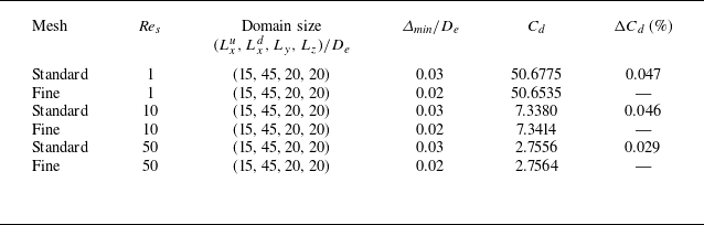
 Cd
 αH=αV=π/3
 G/De=0.1
 ΔCd
 |(Cdstandard−Cdfine)/Cdfine|×100%

 Cf,x=τw,x/((1/2)ρUc2)
 G/De=0.1
 Res=1
 (αH,αV)=(π/3,π/3)
 Δmin/De=0.03
 Δmin/De=0.02
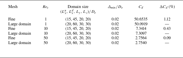
 Cd
 αH=αV=π/3
 G/De=0.1
 Δmin/De=0.02
 ΔCd
 |(Cdfine−Cdlarge\ domain)/Cdlarge\ domain|×100%

 Cd
 Re
 λ=2
 αV=0
 αH
 0
 π/6
 π/4
 π/3
 π/2

 λ=2
 α=0
 α=π/2

 Kwi
 G/De
 (0,0)
 (π/2,0)
 (0,π/2)
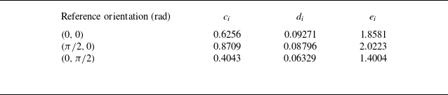
 Kwi

 G/De=0.1
 Res=10
 (0,0)
 (π/2,0)
 (0,π/2)
 x
 y
 x
 z

 αH
 G/De
 Res
 αV=0
 αV=π/4
 αV=π/3
 (Cd−Cd,αH=0)/(Cd,αH=π/2−Cd,αH=0)
 sin2αH

 αV
 G/De
 Res
 Res=1
 αH=0
 Res=10
 αH=0
 Res=10
 αH=π/2

 αV
 G/De
 Cd,v
 Cd,p
 Res=1
 αH=0
 Res=10
 αH=0
 Res=10
 αH=π/2

 Res=10
 G/De=0.1
 (αH,αV)=(0,0)
 (αH,αV)=(0,π/4)
 (αH,αV)=(π/2,0)
 (αH,αV)=(π/2,π/4)

 Cd,DNS
 Cd,Pred
 G/De=0.1
 G/De=1.5

 Cl
 Cm
 G/De
 (αH,αV)=(0,0)
 Cl
 Cm
 αH
 αV=π/4
 Res=1
 Cl
 Cm
 αV
 αH=π/4
 Res=1

 Cd,DNS
 Cd,Pred
 λ=4
 λ=2
 G/De=0.1
 G/De=1.5


