


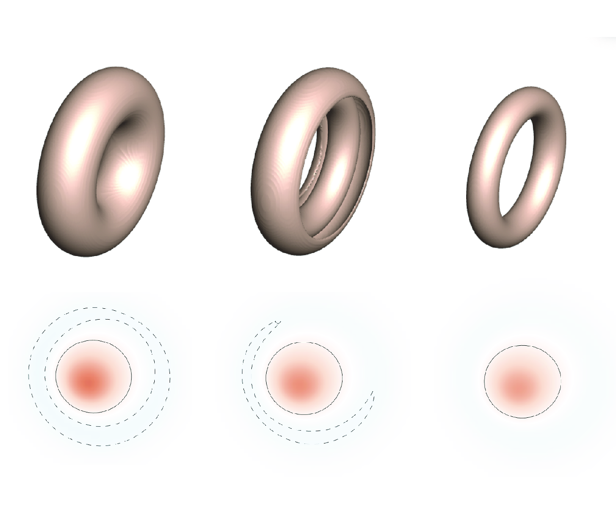

1. Introduction
Vortex rings have been a subject of study for nearly 170 years since Helmholtz (Reference Helmholtz1858), with extensive reviews and books dedicated to this topic (Lugt Reference Lugt1983; Lim & Nickels Reference Lim and Nickels1992; Shariff & Leonard Reference Shariff and Leonard1992; Akhmetov Reference Akhmetov2009; Wu, Ma & Zhou Reference Wu, Ma and Zhou2015). Vortex rings are fundamental elements in complex flows such as turbulence, where they appear in a variety of forms and scales. Their evolution and interaction constitute basic flow mechanisms, influencing flow transport and flow mixing (Shariff, Leonard & Ferziger Reference Shariff, Leonard and Ferziger1989; Shariff & Leonard Reference Shariff and Leonard1992; Green Reference Green1995; Davidson Reference Davidson2015). In nature, vortex rings serve as a highly efficient mechanism for biological propulsion (e.g. Fish & Lauder Reference Fish and Lauder2006; Bartol et al. Reference Bartol, Krueger, Stewart and Thompson2009; Dabiri Reference Dabiri2009). Additionally, the interaction between vortex rings is related to flow-induced sound generation (Kambe & Minota Reference Kambe and Minota1981; Howe Reference Howe2003).
In fundamental study, a vortex ring with extremely small cross-section but finite circulation is often condensed as a loop of vortex filament. According to the Biot–Savart law, a vortex filament with a non-zero circulation induces an infinitely large rotation speed and a self-induced translation speed along its binormal direction proportional approximately to its local curvature as well as the circulation. For a vortex tube with finite thickness, the induced binormal velocity is finite and still influenced by the local curvature. For a circular vortex ring with finite thickness, the curvature along the circumference is constant, resulting in a constant translational speed under inviscid conditions. Determining the magnitude of this speed requires information about the vorticity distribution within the vortex core (Lamb Reference Lamb1932; Fraenkel Reference Fraenkel1970; Saffman Reference Saffman1970; Wu et al. Reference Wu, Ma and Zhou2015). The speed formula for a thin-cored vortex ring having uniform vorticity distribution was first given without proof by Kelvin in an excursus to an English translation of Helmholtz’ paper (Helmholtz Reference Helmholtz1867) by Tait, and later proved by Lamb (Reference Lamb1932). Empirical speed formulas obtained through the energy method for thin-cored vortex rings with arbitrarily prescribed radial vorticity functions were subsequently developed (Lamb Reference Lamb1932; Fraenkel Reference Fraenkel1970; Saffman Reference Saffman1970). A family of general thick-cored vortex rings that bridges the Helmholtz circular vortex filament and the Hill vortex sphere has been found numerically by Norbury (Reference Norbury1973) and proved mathematically by Fraenkel & Berger (Reference Fraenkel and Berger1974). These results all suggest that no matter the self-induction speed of a curved vortex filament or the translational speed of a circular thin-cored vortex ring, the speed is proportional to their circulation, indicating that circulation is a dominant parameter to determine the behaviour of vortex rings.
In addition, the vorticity distribution within the vortex core, and the thickness and the diameter of the vortex ring, are also key factors that affect vortex ring properties. Wu (Reference Wu1993) found that with the same circulation and ring diameter, thinner vortex rings have a greater kinetic energy. With the same circulation, thickness and diameter, different vorticity distributions affect vortex ring properties, such as the kinetic energy, impulse and speed, to a comparably small or a qualitatively consistent degree. On the other hand, the number of waves of instability can be sensitive to the form of the vorticity distribution (Saffman Reference Saffman1978). Typically, vorticity distribution is often assumed Gaussian when studying vortex rings (Saffman Reference Saffman1970). Although linear distribution and uniform distribution are also used sometimes, little attention is paid to vortex rings with other special vorticity distributions. Especially when the thin-cored approximation is not satisfied, the influence of vorticity distribution in more general functions on vortex ring properties remains unrevealed.
For all of the previously studied cases on vortex rings or vortex filament, non-zero circulation is exhibited and even becomes a default prerequisite. However, the circulation of a vortex ring may also be zero in theory. Considering such a possibility, we are sentimentally interested in asking the following questions. What is the evolution if we put a zero-circulation vortex ring into either an ideal or a viscous fluid? Will it endure exceptional evolution? Some qualitative outcomes on the evolution of such vortex rings can be postulated in advance. Overall, the dynamics of vortex rings of zero circulation is expected to be more complex than the behaviour of rings of non-zero circulation. For instance, while steadily propagating inviscid rings, such as the family obtained by Norbury (Reference Norbury1973), exist for single-signed vorticity distributions, this is unlikely to be the case for rings with both positive and negative azimuthal vorticity. One reason for this is that the self-induced velocities of the positive and negative parts are in opposite directions. Note that in the planar case, because there is no self-induced motion, steady flow with circular streamlines is possible even with a sign change in vorticity. However, because Rayleigh’s criterion (that the square of the circulation,
 $\Gamma ^2(r)$
, increases with
 $r$
for centrifugal stability) is violated, centrifugal instability may occur. For very thin rings, the flow in the vicinity of the core is locally planar, and circumferential flow is much more rapid compared to self-induced motion. In this case, a nearly steady flow with nearly circular streamlines and vorticity sign change is possible for many eddy turnover times. However, centrifugal instability cannot be ruled out. For other cases of zero-circulation vortex rings, their behaviour probably depends more on the diverse vorticity distribution. Therefore, the evolution details are hard to infer for a specific zero-circulation vortex ring. Moreover, if the role of fluid viscosity is considered, then the situation is more complicated due to the diffusion of vorticity, and numerical simulation will be more feasible to investigate the evolution of such vortex rings.
Recently, it has been found that there can be a steady solution of the Euler equation within an annular neighbourhood of any circumference, with velocity on and outside the torus being zero (Gavrilov Reference Gavrilov2019). This can be regarded as a zero-circulation vortex ring under ideal conditions (but cannot hold for viscous situations because there exists vorticity discontinuity in this solution). Such a vortex ring will actually levitate quietly in an unbounded motionless ideal fluid without any translation. On the other hand, Yoshida & Giga (Reference Yoshida and Giga1990) proved in mathematics that when zero cross-section flux is satisfied, one can obtain a set of complete and orthogonal discrete eigenfunctions for the curl operator, in any toroidal domain. These eigenfunctions themselves, with swirl, are all the exact steady solutions of the Euler equations and exact decaying solutions for the Navier–Stokes equations, but they are confined to the interior of the toroidal enclosure with zero normal velocity on its boundary domain, unlike the solution of Gavrilov (Reference Gavrilov2019), which is defined on the whole space.
Apart from the theoretical interest, how about the possibility of existence of zero-circulation vortex rings in the real world? First, zero circulation implies that the vorticity distribution of the vortex ring must exhibit oppositely directed vorticity. Finding a circular vortex ring with exactly zero circulation in nature may not be easy, but it may be possible to find ring-shaped vortices containing regions of oppositely signed vorticity with a relatively small net circulation. As can be observed in wake flows produced by swimmers (figure 1), two primary classes of such vortical structures can be identified in the sequential evolution (Hoover et al. Reference Hoover, Griffith and Miller2017, Reference Hoover, Porras and Miller2019; Wei et al. Reference Wei, Hu, Li and Shi2023): the layered and celled vortical structures, respectively. Enlightened by this observation, it can be imagined that zero-circulation vortex rings in three-dimensional space can occur in the wakes of axisymmetric swimmers or other moving objects with axisymmetric compliant trailing edges. It should be emphasised that swimmers have made a wide range of Reynolds numbers in nature (Gazzola, Argentina & Mahadevan Reference Gazzola, Argentina and Mahadevan2014). Moreover, we believe that zero-circulation vortex rings can be achieved experimentally in future. This notion is inspired by one reviewer and will be formally introduced in a later section of the paper.
Instantaneous vorticity contours at two moments in numerical simulations of (
 $a$
) two-dimensional schooling fish swimming (Wei et al. Reference Wei, Hu, Li and Shi2023) and (
 $b$
) three-dimensional oblate jellyfish swimming (see movie 3 in the supplementary materials of Hoover, Porras & Miller Reference Hoover, Porras and Miller2019). Positive and negative vorticity are shown by red and blue, respectively. Two typical patterns, namely the layered vortical structures (in grey boxes) and celled vortical structures (in grey circles), which contain oppositely directed vorticity with a relatively small net circulation, can be identified as the zero-circulation vortical structures in the wake flows.

As the first step of studying zero-circulation vortex rings formally, this work investigated a family of viscous vortex rings with a specially assigned layered vorticity distribution leading to a zero flux of vorticity on the meridian plane or a zero circulation, which is unexplored so far. Such layered vorticity distribution is the simplest structure to achieve zero circulation due to its circular symmetry. Direct numerical simulations are applied to study the evolution of vortex rings from both kinematic and dynamic perspectives. The vortex ring is initially prescribed to be axisymmetric and swirl-free, and there are not the same restrictions imposed later in the computation code. For simplicity in expression, in the following text we alternate the use of the two terms ‘zero-circulation’ and ‘zero-flux’, with equivalent meanings. Herein, ‘flux’ means the vorticity flux through the cross-section of a vortex ring, which is equal to the velocity circulation along any loop enclosing the cross-section.
The paper is organised as follows. Section 2 provides an overview of the direct numerical simulation method and validation. Section 3 reports and analyses the kinematics and dynamics of the zero-circulation viscous vortex rings. Section 4 suggests a possible way to create an approximate layered zero-circulation vortex ring by experiments. Discussion and conclusions are presented in § 5. Two appendices are supplied, for an elucidation on the effect of a finite computational domain, and showing the evolution of a case with exactly zero impulse, respectively.
2. Numerical method
2.1. Direct numerical simulations
To study the evolution and interaction of vortex rings, we directly solve the incompressible Navier–Stokes equations in a periodic cubic box. Compared with the theoretical assumption that the matter happens in unbounded three-dimensional space, the influence caused by periodic boundary conditions is discussed theoretically in Appendix A. The momentum equation is
 \begin{equation} \frac {\partial \boldsymbol{u}}{\partial t}+\boldsymbol{u}\boldsymbol{\cdot} \boldsymbol{\nabla} \boldsymbol{u}=-\frac {1}{\rho }\,\boldsymbol{\nabla} p+\nu\, \boldsymbol{\nabla} ^2\boldsymbol{u}, \end{equation}
and the mass equation is reduced to
 $\boldsymbol{\nabla} \boldsymbol{\cdot} \boldsymbol{u}=0$
. Substituting
 \begin{equation} \boldsymbol{u}\boldsymbol{\cdot} \boldsymbol{\nabla} \boldsymbol{u}=\boldsymbol{\omega }\times \boldsymbol{u}+\boldsymbol{\nabla} \left (\frac {|\boldsymbol{u}|^2}{2}\right) \end{equation}
into the above momentum equation, we obtain the Lamb–Gromeka equation
 \begin{equation} \frac {\partial \boldsymbol{u}}{\partial t}+\boldsymbol{l}=-\boldsymbol{\nabla} \left (\frac {p}{\rho }+\frac {|\boldsymbol{u}|^2}{2}\right)+\nu\, \boldsymbol{\nabla} ^2\boldsymbol{u}, \end{equation}
where
 $\boldsymbol{l}=\boldsymbol{\omega }\times \boldsymbol{u}$
is the Lamb vector. For an arbitrary vector field
 $\boldsymbol{h}(\boldsymbol{x},t)$
in physical space, the Fourier transform is given by
 \begin{equation} \widehat {\boldsymbol{h}}(\boldsymbol{k},t)=\int \boldsymbol{h}(\boldsymbol{x},t)\,\textrm{e}^{-\textrm{i}\boldsymbol{k}\boldsymbol{\cdot} \boldsymbol{x}}\,\text{d}\boldsymbol{x}, \end{equation}
where
 $\boldsymbol{k}(k_x,k_y,k_z)$
is the wavenumber vector in spectral space. Denoting the Fourier transform of
 $\boldsymbol{h}(\boldsymbol{x},t)$
by
 $\widehat {\boldsymbol{h}}(\boldsymbol{k},t)=\mathcal{F}(\boldsymbol{h}(\boldsymbol{x},t))$
, the inverse Fourier transform is
 \begin{equation} \boldsymbol{h}(\boldsymbol{x},t)=\mathcal{F}^{-1}(\widehat {\boldsymbol{h}}(\boldsymbol{k},t))=\frac {1}{(2\unicode{x03C0})^3}\int \widehat {\boldsymbol{h}}(\boldsymbol{k},t)\,\textrm{e}^{\textrm{i}\boldsymbol{k}\boldsymbol{\cdot} \boldsymbol{x}}\,\text{d}\boldsymbol{k}. \end{equation}
Let
 $\boldsymbol{u}=\boldsymbol{h}(\boldsymbol{x},t)$
, and suppose that
 $\boldsymbol{u}$
is sufficiently smooth. Then we have
 \begin{equation} \boldsymbol{\nabla} \boldsymbol{\cdot} \boldsymbol{u}=\boldsymbol{\nabla} \boldsymbol{\cdot} \frac {1}{(2\unicode{x03C0})^3}\int \widehat {\boldsymbol{u}}(\boldsymbol{k},t)\,\textrm{e}^{\textrm{i}\boldsymbol{k}\boldsymbol{\cdot} \boldsymbol{x}}\,\text{d}\boldsymbol{k}=0\Rightarrow i\boldsymbol{k}\boldsymbol{\cdot} \widehat {\boldsymbol{u}}=0, \end{equation}
and the momentum equation in spectral space becomes
 \begin{equation} \frac {\partial \widehat {\boldsymbol{u}}}{\partial t}+\widehat {\boldsymbol{l}}=-i\boldsymbol{k}\,\mathcal{F}\left (\frac {p}{\rho }+\frac {|\boldsymbol{u}|^2}{2}\right)-\nu k^2\widehat {\boldsymbol{u}}, \end{equation}
where
 $k^2\equiv |\boldsymbol{k}|^2$
. Considering the incompressible condition, velocity has a non-zero value only perpendicular to
 $\boldsymbol{k}$
, so (2.7) can be recast as
 \begin{equation} \frac {\partial \widehat {\boldsymbol{u}}}{\partial t}+\widehat {\boldsymbol{l}_{\perp }}=-\nu k^2\widehat {\boldsymbol{u}}, \end{equation}
where
 $\widehat {\boldsymbol{l}_{\perp }}=\widehat {\boldsymbol{l}}-(\widehat {\boldsymbol{l}}\boldsymbol{\cdot} \boldsymbol{k})\boldsymbol{k}/k^2$
. Thus it is sufficient to compute the flow field evolution after having information of the initial velocity field.
Since the input required for directly solving Navier–Stokes equations is the initial velocity field in spectral space, we need to deal with the obtained vorticity field in physical space. Transform the vorticity
 $\boldsymbol{\omega }=\boldsymbol{\nabla} \times \boldsymbol{u}$
into the spectral space version expressed as
 \begin{equation} \widehat {\boldsymbol{\omega }}=i \boldsymbol{k}\times \widehat {\boldsymbol{u}}, \end{equation}
and let
 $\boldsymbol{k}$
cross the above equation. Then we have
 \begin{equation} \boldsymbol{k}\times \widehat {\boldsymbol{\omega }}=\boldsymbol{k}\times (i \boldsymbol{k}\times \widehat {\boldsymbol{u}})=i(\boldsymbol{k}(\boldsymbol{k}\boldsymbol{\cdot} \widehat {\boldsymbol{u}})-k^{2}\widehat {\boldsymbol{u}}). \end{equation}
Here, we force the above equation to satisfy the incompressible condition, so the velocity field in spectral space can be obtained from the vorticity field in spectral space by
 \begin{equation} \widehat {\boldsymbol{u}}=\frac {i \boldsymbol{k}\times \widehat {\boldsymbol{\omega }}}{k^{2}}. \end{equation}
It should be noted that this transformation is valid only for vorticity fields consistent with the divergence-free condition. Evidently, any axially symmetrical vorticity field supported in an axisymmetric ring and having only the azimuthal component is divergence-free.
Based on the designed initial vorticity field and the corresponding velocity field, a pseudo-spectral code is employed to perform the direct numerical simulations on
 $N^3$
grid points. Space and time are discretised by the second-order central difference scheme and second-order Adams–Bashworth scheme, respectively.
2.2. Validation for time step and grid resolution
A periodic box of width
 $2\unicode{x03C0}$
is used to simulate the head-on collision of a pair of vortex rings. We claim that all of the parameters in this work are non-dimensional unless otherwise indicated. Thus actually
 $\rho =1$
is assumed. Convergence issues arose when the grid points increased to
 $256^3$
with time step
 $\Delta t=0.005$
, so we tested smaller time steps
 $\Delta t=0.002$
and
 $\Delta t=0.001$
for circulation Reynolds number (defined as
 $Re_{\Gamma }=\Gamma /\nu$
)
 $Re_{\Gamma }=500$
,
 $1000$
,
 $1500$
,
 $2000$
. Figure 2(
 $a$
) shows the evolution of total enstrophy, which is defined as
 \begin{equation} W=\int \frac {|\boldsymbol{\omega }|^2}{2}\,\text{d}V. \end{equation}
Unless otherwise specified,
 $*$
in the present work denotes the normalised form of the quantity based on its initial value.
We took the results for
 $\Delta t=0.001$
as reference, then calculated the relative errors of the results for
 $\Delta t=0.002$
. For these four cases with different circulation Reynolds numbers, the relative errors of maximum total enstrophy are
 $0.02\, \%$
,
 $0.02\, \%$
,
 $0.10\, \%$
and
 $0.28\, \%$
, respectively. It could be seen that within the selected range of circulation Reynolds numbers, decreasing the time step improved accuracy slightly. To decide the resolution, we took the results for
 $N^3=512^3$
as a reference, and simulated cases with resolution
 $N^3=128^3$
and
 $256^3$
for the four circulation Reynolds numbers as mentioned before. The results of total enstrophy evolution are plotted in figure 2(
 $b$
). The relative errors of maximum total enstrophy for
 $N^3=128^3$
are
 $2.51\, \%$
,
 $3.57\, \%$
,
 $5.66\, \%$
and
 $7.78\, \%$
, while for
 $N^3=256^3$
they are
 $0.60\, \%$
,
 $0.85\, \%$
,
 $1.16\, \%$
and
 $1.59\, \%$
. As a result, we took
 $\Delta t=0.002$
and
 $N^3=256^3$
for further simulations.
Evolution of total enstrophy for validation of (
 $a$
) time step and (
 $b$
) grid resolution. Blue markers and black lines in (
 $a$
) are the results for time steps
 $\Delta t=0.002$
and
 $\Delta t=0.001$
, respectively. In (
 $b$
), there are three different kind of grid resolutions, namely the grid points
 $N^3=128^3$
,
 $256^3$
and
 $512^3$
, results of which are represented by the blue, red and black lines, respectively.

The trend of total enstrophy matches results from Chu et al. (Reference Chu, Wang, Chang, Chang and Chang1995), reflecting key physical mechanisms in three stages of head-on collisions. In the free-travelling stage, the mutual induction effect is not apparent, so the vortex core centre has an approximately translational motion under self-induction. During this period, the effect of the convection term is significantly greater than that of the viscosity term. The total enstrophy shows a slow downward trend under slow vorticity diffusion. In the stage of vortex stretching, the effect of mutual induction gradually plays an important role. The vortex ring becomes thinner while the total flux remains almost constant (because the total flux is a conserved quantity), which leads to a rapid enhancement of vorticity intensity through vorticity stretching. This process causes a sharp increase in total enstrophy. In the viscosity-dissipating stage, the vortex rings become very slender, and the radial growth rate gradually slows down. During this stage, the viscous effect dominates and the total enstrophy will decrease.
2.3. Comparisons with previous works
To verify the reliability of numerical simulations, we simulated oblique collisions and compared the results with Kida, Takaoka & Hussain (Reference Kida, Takaoka and Hussain1991). The vorticity distribution function on the meridian plane of each vortex ring is
 \begin{equation} \omega (r)=\omega _0\, \text{e}^{-r^2/a^2}, \end{equation}
where
 $\omega _0=23.8$
and
 $a$
are constants, and
 $r$
is the radial coordinate of the local polar coordinate on the meridian plane, with the coordinate origin located at the vortex core centre. To avoid infinitely large core radius, we truncate at
 $|\boldsymbol{\omega }|=0.01 \omega _0$
, setting
 $|\boldsymbol{\omega }|=0$
outside this region (i.e.
 $r\gt r_0$
). The relationship between
 $a$
and
 $r_0$
is
 $a=\sqrt {-r_0^2/\ln0.01}$
.
Figure 3 shows the initial geometry of oblique collisions. We simulated the cases
 $\beta =0^{\circ }$
and
 $\beta =45^{\circ }$
, with parameters matching
 $\text{Case}\,\textrm{II}$
and
 $\text{Case}\,\textrm {V}$
in Kida et al. (Reference Kida, Takaoka and Hussain1991). The kinematic viscosity is taken as
 $\nu =0.005$
, and the circulation Reynolds number is
 $Re_{\Gamma }=577$
. Figure 4 shows qualitatively identical comparison results, confirming the reliability of our simulations.
Initial vorticity isosurface (
 $|\boldsymbol{\omega }|=0.01 \omega _0$
) of oblique collisions: (a) full view, (b) front view. Here,
 $D=1.83$
is the distance between two ring centres,
 $R_0=0.491$
and
 $r_0=0.422$
are the initial ring and core radii, respectively, and
 $\beta$
is the acute angle between the vorticity loop and the
 $x{-}y$
plane. The black solid lines show the boundary of the periodic box.

The evolution of the vorticity isosurface for oblique collisions. Columns (A) and (B) compare the results of this work and
 $\text{Case}\,\textrm {II}$
of Kida et al. (Reference Kida, Takaoka and Hussain1991) for
 $\beta =0^{\circ }$
. Columns (C) and (D) compare the results of this work and
 $\text{Case}\,\textrm {V}$
of Kida et al. (Reference Kida, Takaoka and Hussain1991) for
 $\beta =45^{\circ }$
. (A,B) Here, (
 $a_{1}$
)
 $t=0,\ |\boldsymbol{\omega }|=0.4\,|\boldsymbol{\omega }|_{{max}}$
, (
 $b_{1}$
)
 $t=3,\ |\boldsymbol{\omega }|=0.4\,|\boldsymbol{\omega }|_{{max}}$
, (
 $c_{1}$
)
 $t=4.5, |\boldsymbol{\omega }|=0.5|\boldsymbol{\omega }|_{{max}}$
, (
 $d_{1}$
)
 $t=6, |\boldsymbol{\omega }|=0.4|\boldsymbol{\omega }|_{{max}}$
, (
 $e_{1}$
)
 $t=7.5, |\boldsymbol{\omega }|=0.5|\boldsymbol{\omega }|_{{max}}$
, (
 $f_{1}$
)
 $t=12, |\boldsymbol{\omega }|=0.4|\boldsymbol{\omega }|_{{max}}$
, (
 $g_{1}$
)
 $t=18, |\boldsymbol{\omega }|=0.4|\boldsymbol{\omega }|_{{max}}$
. (C,D) Here, (
 $a_{2}$
)
 $t=0, |\boldsymbol{\omega }|=0.4|\boldsymbol{\omega }|_{{max}}$
, (
 $b_{2}$
)
 $t=1.5, |\boldsymbol{\omega }|=0.4|\boldsymbol{\omega }|_{{max}}$
, (
 $c_{2}$
)
 $t=3, |\boldsymbol{\omega }|=0.4|\boldsymbol{\omega }|_{{max}}$
, (
 $d_{2}$
)
 $t=4.5, |\boldsymbol{\omega }|=0.5|\boldsymbol{\omega }|_{{max}}$
, (
 $e_{2}$
)
 $t=6, |\boldsymbol{\omega }|=0.5|\boldsymbol{\omega }|_{{max}}$
, (
 $f_{2}$
)
 $t=7.5, |\boldsymbol{\omega }|=0.5|\boldsymbol{\omega }|_{{max}}$
, (
 $g_{2}$
)
 $t=10.5, |\boldsymbol{\omega }|=0.4|\boldsymbol{\omega }|_{{max}}$
. (Regarding the typographical errors in Kida et al. (Reference Kida, Takaoka and Hussain1991): the first three images of (c) and (d) in figure 20 of their paper are mixed up. Modifications have been made here).

2.4. Layered zero-flux vortex rings
We consider an initial swirl-free axisymmetric circular vortex ring in the three-dimensional homogeneous and incompressible laminar flow. The initial geometry of a vertically placed vortex ring is shown in figure 5. The initial vorticity distribution
 $\omega (r)$
of a swirl-free vortex ring is prescribed on the meridian plane of the vortex ring as
 \begin{equation} \omega (r)=\frac {\sin(2\unicode{x03C0} n r/r_{0})}{r},\quad n=1,2,3,\ldots, \end{equation}
where
 $r_{0}$
is the radius of the vorticity boundary, i.e. the radius of the core of the vortex ring, and
 $n$
represents the number of positive/negative vorticity layers. It is simple to verify that this vorticity field is divergence-free. The initial total circulation on the meridian plane is
 \begin{equation} \Gamma =\int _{\text{0}}^{r_{\text{0}}}\!\!\int _{\text{0}}^{\text{2}\unicode{x03C0} }\frac {\sin(\text{2}\unicode{x03C0} n r/r_{\text{0}})}{r}\, r\,\text{d}\phi\, \text{d} r =-\frac {r_{\text{0}}}{n} \cos\left.\left (\frac {\text{2}\unicode{x03C0} n r}{r_{\text{0}}}\right)\right |_{\text{0}}^{r_{\text{0}}}=\text{0}. \end{equation}
This kind of vorticity distribution has a layered pattern, so we simply term such vortex rings as ‘layered zero-flux vortex rings’.
The vortical impulse of such a zero-flux vortex ring is to be investigated. The total vortical impulse is defined as
 \begin{equation} \boldsymbol{I}=\tfrac{1}{2}\int \boldsymbol{x}\times \boldsymbol{\omega }\,\text{d}V, \end{equation}
where
 $\boldsymbol{x}$
is the position vector. Due to the axisymmetry, the initial total vortical impulse has only an axial component
 $I$
:
 \begin{align} I &=\unicode{x03C0} \int _{\text{0}}^{r_{\text{0}}}\int _{\text{0}}^{\text{2}\unicode{x03C0} }\sigma ^2\,\omega (r)\,r\,\text{d}\phi\, \text{d} r\notag \\ &=\unicode{x03C0} \int _{\text{0}}^{r_{\text{0}}}\int _{\text{0}}^{\text{2}\unicode{x03C0} }(R+r\cos\phi)^2\frac {\sin(\text{2}\unicode{x03C0} n r/r_{\text{0}})}{r}\,r\,\text{d}\phi\, \text{d} r=-\frac {\unicode{x03C0} r_0^3}{2n}. \end{align}
Compared with ordinary vortex rings of non-zero circulation, the following points for the layered zero-flux vortex rings should be emphasised based on (2.17).
-
(i) Their impulse cannot be influenced by the ring radius
 $R$
. In other words, the line momentum of the flow field generated by the vortex ring is irrelevant to the size of the vortex ring. This property is non-trivial, and it actually exists not only for vorticity distribution regulated as (2.14), but also for all layered zero-flux vorticity distributions, satisfying(2.18)In particular, the vortex ring can be of zero impulse if
\begin{equation} \boldsymbol{\omega }=\omega (r)\,\boldsymbol{e}_\theta,\quad \int _{0}^{r_{\text{0}}}r\,\omega (r)\,\text{d}r=0. \end{equation}
$\omega (r)$
satisfies
$ \int _{0}^{r_{\text{0}}}r^2\,\omega (r)\,\text{d}r=0$
in addition to (2.18).
-
(ii) Their impulse is rather small compared with the thin-cored case of an ordinary vortex ring, for which we have
$I=O(r_{\text{0}}^2 R)$
. This is due to the coexistence of both positive and negative vorticity layers. Therefore, the motion of the whole vortex ring may be very weak. This can be an important feature of the layered zero-flux vortex rings. -
(iii) When
$n\to \infty$
, we have
$I\to 0$
. The reason is similar to that in (ii).


To further investigate the influence of impulse, a case of such a layered zero-flux vortex ring with exactly zero impulse is given in Appendix B.
Geometric sketch of a vertically placed vortex ring in Cartesian coordinates
 $(x,y,z)$
or cylindrical coordinates
 $(\sigma,\theta,y)$
. Here,
 $(r,\phi)$
are the local polar coordinates on the meridian plane, and
 $R$
and
 $r_0$
are the ring and core radii, respectively.

In the present work, the geometric parameters of the vortex ring are taken as
 $R_{0}=1$
and
 $r_{0}=0.5$
. Therefore, the relative vortex core radius (i.e. aspect ratio) is
 $r_{0}/R_{0}=0.5$
, for which the thin-cored approximation (
 $r_{0}/R_{0}\ll 1$
) is no longer applicable, and theoretical analysis is difficult to carry out. But for convenience, we can still apply the assumption of a circular cross-section to the initial vortex ring. The initial vorticity distributions along the azimuthal direction on any meridian plane are plotted in figure 6. The free parameter
 $n$
is selected as
 $1,2,3,5$
, respectively. Also,
 $\nu$
is taken as
 $0.005$
, i.e. the natural Reynolds number is
 $Re=1/\nu =200$
in the present work. A remarkable observation that we obtained is the fact that vortex rings with zero flux in the present work can preserve both the axial symmetry and the nature of no swirl, which are not imposed in the numerical code, during the entire period of the simulation. Therefore, most of the following analyses are completed in a certain meridian plane of the axial-symmetry-preserved vortex ring.
Distribution of the azimuthal vorticity at initial moment on the meridian plane for cases
 $n=1,2,3,5$
.

3. Results and analysis
3.1. Evolution of the flow field
3.1.1. Vorticity distribution
To find the position of the vortex core centre, we integrated the squared vorticity along the
 $y$
and
 $z$
directions within the area
 $S$
given by
 $x=0$
,
 $y\in [-\unicode{x03C0},\unicode{x03C0}]$
,
 $z\in [0,\unicode{x03C0}]$
:
 \begin{equation} q_{y}=\int _0^{\unicode{x03C0} } |\boldsymbol{\omega }|^{2}\,\text{d}z,\quad q_{z}=\int _{-\unicode{x03C0} }^{\unicode{x03C0} } |\boldsymbol{\omega }|^{2}\,\text{d}y, \end{equation}
where
 $|\boldsymbol{\omega }|^{2}=\omega ^{2}_{x}+\omega ^{2}_{y}+\omega ^{2}_{z}$
. Then we find the
 $y$
and
 $z$
coordinates where
 $q_y$
and
 $q_z$
reach their extrema, respectively. A subsequent three-point Gaussian smoothing locates the unique axial and radial positions corresponding to the maximum integrated square vorticity. This point is identified as the centre of the vortex core. Based on this position, the (azimuthal) vorticity distributions along a
 $z$
-directional line passing the vortex core centre at different moments are plotted in figure 7. It can be seen that compared to the main peak vorticity, secondary peaks are smoothed in a very short time. (For convenience, we refer to the peak where the maximum vorticity is located as the main peak, and the rest as the secondary peak.) Especially for cases
 $n=2,3,5$
, the layered structures with alternating positive and negative vorticity reorganise into a smoother distribution very soon. The larger
 $n$
, which means more layers, the higher the initial decay rate of the main peak vorticity. It is natural to make a relation with viscosity, as it has a tendency to uniformise the vorticity field. According to the form of the viscous term
 $\nu\, \boldsymbol{\nabla} ^2 \boldsymbol{u}$
in the Navier–Stokes equation, the viscous effect is related to the first-order spatial derivative of the vorticity distribution.
Evolution of the distribution of the azimuthal vorticity along a
 $z$
-directional line passing the vortex core centre: (a)
 $n=1$
, (b)
 $n=2$
, (c)
 $n=3$
, (d)
 $n=5$
.

3.1.2. Instantaneous streamline pattern and velocity distribution
Streamlines and velocity contours are plotted in figure 8 to show the flow field evolution. From the streamline patterns, the far-field part of layered zero-flux vortex rings is similar to vortex rings with Gaussian distribution, but the near-field patterns are completely different. At the initial moment (
 $t=0$
), it can be seen that all cases have a unified structure, namely the closed streamline area at and outside the velocity concentration zone, which is the key to achieving zero flux. The zero-flux characteristic requires that on any meridian plane, the circulation is zero, so these two closed streamline areas have opposite directions. The innermost vortex ring carrying main peak vorticity has properties similar to an ordinary vortex ring with non-zero circulation, affecting the near-field fluids. When flow fields begin to evolve (
 $t=2.4,4.8$
), due to the self-induction of the innermost vortex rings, the closed streamline areas with considerably greater velocities tend to grow along the direction of vortex ring motion. The trend of growth slows down as the number of layers increases, possibly due to more and more weak influence of the innermost vortex rings, as shown by the dashed areas in figure 8.
Streamline patterns on the meridian plane
 $x=0$
of cases
 $n=1,2,3,5$
at
 $t=0.0, 2.4, 4.8$
. Backgrounds are velocity contours. The area surrounded by the dashed black line is the maximum closed streamline area containing considerably greater velocities.

Through careful observation of figure 8, it can be reasonable to assume that velocity has only a component along the
 $\phi$
direction near the vorticity core centre on each meridian plane. Therefore, we may obtain an approximation of the initial velocity distribution through the vorticity distribution. Since
 $\omega _\theta$
is the only non-zero component of the vorticity field, we have
 $\omega _\theta \approx \partial (r u_\phi)/r\,\partial r$
on the region with strongest velocities on any meridian plane. Substituting (2.14) into the approximate expression of vorticity, we can obtain an equation concerning velocity,
 \begin{equation} \frac {\sin(2\unicode{x03C0} n r/r_{0})}{r}\approx \frac {1}{r}\frac {\partial (r u_\phi)}{r\,\partial r}, \end{equation}
which yields
 \begin{equation} u_\phi \approx \frac {r_{0}}{2\unicode{x03C0} n r}\left (1-\cos\frac {2\unicode{x03C0} n r}{r_{0}}\right). \end{equation}
From this equation, it can be seen that on any meridian plane the velocity distribution is also layered, which is consistent with the velocity contours in figure 8.
A two-dimensional infinite plane can be mapped into a Riemannian sphere through stereo projection, with the north pole of the sphere corresponding to infinity. The Poincaré index theorem states that the index sum of fixed points for any continuous vector field on a sphere should be
 $2$
. It is easy to verify that for a circular vortex filament, the cross-section streamline has two centres on the sphere after being mapped, so the index sum is
 $2$
. For the cross-section streamline of a vortex ring with a Gaussian distribution under periodic boundary conditions, the sum of the near-field fixed point index is also
 $2$
. However, because of the influence brought about by periodic boundary conditions, there are two additional saddles in each periodic area (four half-saddles on the boundary at the initial moment), so the index sum within the periodic area is
 $0$
. For streamline patterns of a layered zero-flux vortex ring, the topological characteristics are clearly different from ordinary vortex rings. We select the instantaneous streamline pattern of case
 $n=2$
at
 $t=4.8$
for illustration, as shown in figure 9. Without considering the impact of boundary conditions, it can be seen that the index sum of zero-flux vortex rings also satisfies the index theorem, but is more complex compared to ordinary vortex rings. Due to the coexistence of anti-sign circulation areas, there exist two saddles and four centres. Unlike the separation of wall-attached flows, there is no source or sink in incompressible vortical flows, so the separation line starts from a saddle point and terminates at another saddle point rather than a node. Although the magnitude in the outer closed streamline area is very small, as can be seen from the velocity contours, the far-field fluids still contribute to flow properties. This area exists mainly due to the layered secondary vorticity structures, as an overall feature that offsets the influence from the main peak vorticity.
Instantaneous streamline pattern of case
 $n=2$
at
 $t=4.8$
on plane
 $x=0$
. Background is the velocity contour. The black dots represent saddles generated by periodic boundary conditions, the red dots represent original saddles of the flow field, and the yellow dots represent centres. The thick black solid line in the middle represents the separation line, and the area enclosed by the dashed line corresponds to the innermost vortex ring. Here,
 $\pm 1$
represents the index corresponding to the fixed point.

3.2. The characteristics of vortical structures
Before using the concept of ‘vortex’, it is necessary to clarify that there is so far no clear definition of vortex in a viscous fluid, so it is impossible to accurately identify viscous vortex rings. There are various opinions on the definition of a vortex, such as those of Saffman & Baker (Reference Saffman and Baker1979), Lugt (Reference Lugt1983), Green (Reference Green1995) and Wu, Xiong & Yang (Reference Wu, Xiong and Yang2005). From the streamline patterns in § 3.1.2, it can be seen that if a velocity field is used to identify vortical structures, then the flow field could actually be regarded as a composition of two vortex rings: the inner-side and outer-side closed streamline areas. For convenience, we still identify vortex structures through a vorticity field, which is the most common way. Although from the perspective of a vorticity isosurface, the zero-flux layered vortex ring is of the same topology as an ordinary vortex ring, its vorticity distribution or vortical structure could be totally different and need to be visualised.
3.2.1. The evolution of layered vorticity structures within the vortex core
We take the meridian plane
 $x=0,\ z\lt 0$
for analysis. On this plane, the vorticity vector has a non-zero component only along the
 $x$
direction, and the main peak vorticity is positive. We consider the region
 $|\boldsymbol{\omega }|\gt 0.01\,|\boldsymbol{\omega }|_{{max}}$
as the effective volume of the vortex ring, where
 $|\boldsymbol{\omega }|_{{max}}$
is the maximum vorticity magnitude of the initial vorticity field.
Vorticity contours on the meridian plane for
 $n=1$
at typical moments. The solid line represents the boundary of the positive vorticity area at
 $\omega _x=0.01\,|\boldsymbol{\omega }|_{{max}}$
, and the dashed line represents the boundary of the negative vorticity area at
 $\omega _x=-0.01\,|\boldsymbol{\omega }|_{{max}}$
. Times are (a)
 $t=0$
, (b)
 $t=0.8$
, (c)
 $t=1.6$
, (d)
 $t=2.4$
, (e)
 $t=4.0$
, (f)
 $t=4.8$
.

Figure 10 shows the evolution of vorticity contours when
 $n=1$
. At the beginning stage of evolution, the main peak vorticity undergoes a rapid decay, and the innermost vortex ring that holds it has a self-induced velocity, causing the vortex core centre to translate (figure 10
 $a{-}c$
). A shell structure is formed in the late stage of evolution, in which the innermost vortex ring is wrapped by an external negative vorticity area, as can be seen from figure 10(
 $d{-}\!f$
). The external negative vorticity area is similar to a hollow vortex ring, while the internal hollow area contains an ordinary vortex ring with positive vorticity, and there is also a weak-vorticity gap between two areas, indicating that the vorticity field is very smooth. Although the motion of the internal vortex ring is weak in the axial direction due to the limitation of the external vorticity region, it evolves like an ordinary vortex ring. From figure 10(
 $a{-}\!f$
), it can be seen that the whole vortex ring has a significant trend to become thicker. This is because vorticity diffusion leads to the homogenisation of the vorticity field, causing the vortex core to gradually thicken. When the boundary of the vortex core is considered as
 $|\boldsymbol{\omega }|=0.1\,|\boldsymbol{\omega }|_{{max}}$
, a cracking process of the shell structure can be observed, as shown in figure 11. During this process, the outer-side vorticity structure carrying opposite vorticity gradually disappears under the action of vorticity diffusion and cancellation, exposing the inner-side vortex ring.
Vorticity isosurfaces
 $|\boldsymbol{\omega }|=0.1\,|\boldsymbol{\omega }|_{{max}}$
and vorticity contours on the meridian plane for
 $n=1$
at typical moments. There are two surfaces from (a) to (e). The solid line represents the boundary of the positive vorticity area at
 $\omega _x=0.1\,|\boldsymbol{\omega }|_{{max}}$
, and the dashed line represents the boundary of the negative vorticity area at
 $\omega _x=-0.15\,|\boldsymbol{\omega }|_{{max}}$
. Times are (a)
 $t=0.8$
, (b)
 $t=0.88$
, (c)
 $t=0.96$
, (d)
 $t=1.04$
, (e)
 $t=1.12$
, (f)
 $t=2.04$
.

Figure 12 shows the evolution of vorticity contours when
 $n=2$
. At the initial stage, the vorticity field maintains its original structure, but the peak vorticity rapidly decays (figure 12
a,b). When the vortex core centre moves, the symmetry of vorticity distribution on the meridian plane is broken. Then the presence of a larger vorticity gradient in the direction of vortex centre movement leads to stronger cancellation of positive and negative vorticity. Therefore, during the vortex centre movement, vorticity of layered structures is continuously transported to the forward direction of the vortex core to supplement the vorticity consumed. This seems to be an ‘unshell’ process of the vortex ring, as can be seen in figure 12(
 $c$
). This process is driven by the starting of the innermost vortex ring carrying main peak vorticity, going layer by layer from the inside out. In addition, vorticity fusion occurs between multi-layer structures because of the insufficient vorticity cancellation (figure 12
c,d). In the late stage, vorticity cancellation causes the negative vorticity area to break apart at the place with a larger vorticity gradient. After the outermost shell disappears, only the positive vorticity area is left as a vorticity concentration area (figure 12
e,f).
Vorticity contours on the meridian plane for
 $n=2$
at typical moments. The solid line represents the boundary of the positive vorticity area at
 $\omega _x=0.01\,|\boldsymbol{\omega }|_{{max}}$
, and the dashed line represents the boundary of the negative vorticity area at
 $\omega _x=-0.01\,|\boldsymbol{\omega }|_{{max}}$
. Times are (a)
 $t=0$
, (b)
 $t=0.40$
, (c)
 $t=0.84$
, (d)
 $t=0.96$
, (e)
 $t=4.40$
, (f)
 $t=4.80$
.

Vorticity contours on the meridian plane for
 $n=3$
at typical moments. The solid line represents the boundary of the positive vorticity area at
 $\omega _x=0.01\,|\boldsymbol{\omega }|_{{max}}$
, and the dashed line represents the boundary of the negative vorticity area at
 $\omega _x=-0.01\,|\boldsymbol{\omega }|_{{max}}$
. Times are (a)
 $t=0$
, (b)
 $t=0.28$
, (c)
 $t=0.36$
, (d)
 $t=0.40$
, (e)
 $t=0.80$
, (f)
 $t=3.20$
.

Figure 13 shows the evolution of vorticity contours when
 $n=3$
. Similar to case
 $n=2$
, during the initial stage, peak vorticity rapidly decays with its structure maintained (figure 13
a,b). Afterwards, when the movement of the vortex core centre begins, the negative vorticity area outside the innermost vortex ring is ‘unshelled’ due to vorticity cancellation (figure 13
b,c). Then vorticity fusion occurs between the innermost and outer-side positive vorticity areas (figure 13
c,d). At the same time, it can be seen that when there is interaction between the main peak and adjacent vorticity areas, the further positive vorticity area is also cancelled (figure 13
 $d$
), ultimately forming a shell structure with the outer-side negative vorticity area surrounding the inner-side positive vorticity area (figure 13
 $e$
). The intermediate layered structures are all diffused and cancelled by the interaction during this process. After that, there is a weak vorticity gap between the outside hollow vortex ring carrying negative vorticity and the inside vortex ring carrying positive vorticity. Subsequently, the vortex ring carrying main peak vorticity continues to thicken under the action of viscosity until vorticity cancellation occurs with the outside negative vorticity area (figure 13
e,f).
Figure 14 shows the evolution of vorticity contours when
 $n=5$
. As the number of layers increases, the influence of main peak vorticity weakens, and the interaction among layered vorticity structures strengthens. In the initial stage, there is also a rapid decay process (figure 14
a,b), but this stage is very short compared to the cases mentioned above. The multi-layered structures have extremely large vorticity gradients, resulting in strong interactions among layered structures. Sufficient vorticity cancellation occurs in a short period of time, leaving only the structure with the outer-side negative vorticity area surrounding the inner-side positive vorticity area. This process is driven by the effect that viscosity will gradually flatten the entire vorticity field through diffusion and cancellation, which is especially significant in areas with large vorticity gradients. It can be seen that there is a large gap of weak vorticity area between the negative and positive vorticity areas after sufficient vorticity cancellation (figure 14
 $c$
). Subsequently, the vortex ring carrying main peak vorticity slowly evolves, while the outer-side hollow vortex ring gradually diffuses (figure 14
 $d{-}\!f$
).
Vorticity contours on the meridian plane for
 $n=5$
at typical moments. The solid line represents the boundary of the positive vorticity area at
 $\omega _x=0.01\,|\boldsymbol{\omega }|_{{max}}$
, and the dashed line represents the boundary of the negative vorticity area at
 $\omega _x=-0.01\,|\boldsymbol{\omega }|_{{max}}$
. Times are (a)
 $t=0$
, (b)
 $t=0.08$
, (c)
 $t=0.40$
, (d)
 $t=1.56$
, (e)
 $t=1.68$
, (f)
 $t=4.80$
.

Overall, the evolution of layered zero-flux vortex rings has a certain regularity and can be divided mainly into four stages: peak-vorticity-weakening stage, internal-interaction stage, shell-structure stage and free-travelling stage. In the first stage, the main process is the weakening of peak vorticity under viscous effect. The second stage is the interaction among layered vorticity structures, which mainly includes two mechanisms: vorticity cancellation and fusion. When the interaction is fully completed, the vortex ring with initial layered vorticity field becomes a shell structure and enters the third stage, which is a relatively smooth process. The whole shell structure evolves until the outer-side area carrying opposite vorticity is cancelled by the inner-side vorticity area. Ultimately, the vortex ring degenerates into an ordinary vortex ring, and the subsequent evolution is the fourth stage. It is worth noting that the entire evolution process is basically confined to a limited area, and the vortex ring motion is very inconspicuous.
3.2.2. The expansion and contraction of the vortex ring volume
In order to identify the different stages of flow field evolution more clearly, we investigated the evolution of vortex ring volume that is defined in § 3.2.1 and represents the volume of concentrated vorticity. The results are shown in figure 15. The four stages mentioned in the previous subsubsection can be clearly distinguished from this figure. For case
 $n=1$
, due to the absence of an internal-interaction stage, the volume of the vortex ring first increases in the peak-vorticity-weakening stage, then decreases due to the cancellation of vorticity between the innermost vortex ring and the outer-side vorticity area. For cases
 $n=2,3,5$
, the curves exhibit a similar trend. The first stage of growth is brought by the peak-vorticity-weakening stage, then due to sufficient interaction among layered structures, vorticity cancellation leads to a drop in volume, forming a shell structure. Subsequently, the evolution of the shell structure leads to an increase in volume due to vorticity diffusion. When it reaches a certain level, the process of vortex cancellation begins again, causing the volume to decrease, and ultimately leaving only the vortex ring carrying main peak vorticity to evolve independently.
The evolution of the vortex ring volume. The purple segment
 $\textrm {I}$
represents the peak-vorticity-weakening stage, the orange segment
 $\textrm {II}$
represents the internal-interaction stage, the green segment
 $\textrm {III}$
represents the shell-structure stage, and the blue segment
 $\textrm {IV}$
represents the free-travelling stage.

3.2.3. The motion of the vortex core centre
Figure 16 shows trajectories of the vortex core centre and the evolution of velocity magnitude and its components yielded from trajectories. The velocity magnitude and its components are normalised by initial velocity magnitude. The seven marked points from left to right on the curve of figure 16(
 $a$
) correspond to the position of the vortex core centre at times
 $t=0,0.8,1.6,2.4,3.2,4.0,4.8$
, respectively. Overall, vortex rings with different
 $n$
all have an axial self-induced velocity, indicating that although the circulation of layered zero-flux vortex rings vanishes, they cannot remain stationary due to the small vortical impulse. Intuitively, this velocity clearly comes from the innermost vortex ring carrying main peak vorticity. With more vorticity layers inside the vortex core, the circulation of the innermost vortex ring is then smaller. As a result, the self-induced velocity exhibited by the case with larger
 $n$
is smaller, as can be seen in figure 16(
 $a$
). For ordinary vortex rings, under the action of viscosity, they will gradually become thicker, their radius will increase, and then the self-induced velocity will decrease. But the radii of layered zero-flux vortex rings first increase and then decrease. This trend approaches completely degenerating into a decreasing trend when
 $n$
is larger. For example, in case
 $n=5$
, it is almost impossible to see an increase in radius. From figure 16(
 $b$
), one can see that the velocity of the vortex core centre is mainly dominated by the axial self-induced velocity, but the impact of radial velocity cannot be neglected, which causes a visible movement of the vortex core centre in the radial direction. In the late stage of evolution, vortex core centres seem to have a steady motion, as can be seen in both figures 16(
 $a$
) and 16(
 $b$
).
The motion of the vortex core centre, where the
 $*$
denotes the normalised form based on initial
 $|\boldsymbol{u}|$
: (a) trajectories, (b) evolution of velocity magnitude and its components.

3.3. Evolution characteristics of some integral quantities
3.3.1. Total enstrophy
Evolution of (a) total enstrophy and (b) total kinetic energy. Here,
 $\alpha$
and
 $\beta$
are fitting power exponents of
 $W^{*}$
and
 $K^{*}$
in the late stage of evolution, respectively.

Figure 17(
 $a$
) shows the evolution of total enstrophy. Typically, an ordinary vortex ring evolves under slow vorticity diffusion until vorticity cancellation occurs at the axis. What is different from an ordinary vortex ring is that in the evolution of a zero-flux layered vortex ring, strong internal interaction happens at the initial stage, which causes strong vorticity cancellation and diffusion, especially for larger
 $n$
. Therefore, the decay of total enstrophy of zero-flux vortex rings is more rapid than for ordinary vortex rings. Particularly at the internal-interaction stage, the evolution of total enstrophy shows a sharp decay compared to other stages, which can be observed as the higher decay rate of total enstrophy during
 $10^{-2}\lt t\lt 10^{0}$
. When the interaction between layered vorticity structures is fully completed, the decay rate of total enstrophy recovers to the former level (
 $t\gt 10^{0}$
), as can be seen in figure 17(
 $a$
). In the late stage, the evolution of total enstrophy decays with an approximate power law
 \begin{align} W^{*}\sim t^{-1.8\pm 0.1}. \end{align}
For homogeneous and incompressible flows without external force, the vorticity dynamics equation becomes
 \begin{equation} \frac {d \boldsymbol{\omega }}{\text{d}t}=\boldsymbol{\omega }\boldsymbol{\cdot} \boldsymbol{\nabla} \boldsymbol{u}+\nu\, \boldsymbol{\nabla} ^{2}\boldsymbol{\omega }. \end{equation}
The dot product of the vorticity vector with the above equation yields
 \begin{equation} \frac {\text{d}}{\text{d}t}\left (\frac {|\boldsymbol{\omega }|^{2}}{2}\right)=\boldsymbol{\omega }\boldsymbol{\cdot} \boldsymbol{\nabla} \boldsymbol{u}\boldsymbol{\cdot} \boldsymbol{\omega }+\nu \boldsymbol{\omega }\boldsymbol{\cdot} \boldsymbol{\nabla} ^{2}\boldsymbol{\omega }. \end{equation}
Substituting
 $\boldsymbol{\nabla} \boldsymbol{u}=\mathbb{D}+\mathbb{A}$
and
 $\boldsymbol{\nabla} ^{2}\boldsymbol{\omega }=-\boldsymbol{\nabla} \times (\boldsymbol{\nabla} \times \boldsymbol{\omega })$
into (3.6), where
 $\mathbb{D}$
is the symmetric strain rate tensor, and
 $\mathbb{A}$
is the anti-symmetric rotation tensor, we have
 \begin{equation} \frac {\text{d}}{\text{d}t}\left (\frac {|\boldsymbol{\omega }|^{2}}{2}\right) = \boldsymbol{\omega }\boldsymbol{\cdot} \mathbb{D}\boldsymbol{\cdot} \boldsymbol{\omega }-\nu \boldsymbol{\omega }\boldsymbol{\cdot} \boldsymbol{\nabla} \times \boldsymbol{\nabla} \times \boldsymbol{\omega }. \end{equation}
Integrating the above equation over the periodic box, we can obtain
 \begin{equation} \frac {\text{d}W}{\text{d}t}=\frac {\text{d}}{\text{d}t}\int \frac {|\boldsymbol{\omega }|^{2}}{2}\,\text{d}V =\int \left (\lambda _1\omega _x^2+\lambda _2\omega _y^2+\lambda _3\omega _z^2\right)\,\text{d}V-\nu \int |\boldsymbol{\nabla} \times \boldsymbol{\omega }|^{2}\,\text{d}V, \end{equation}
where
 $\lambda _1,\lambda _2,\lambda_3$
are the three eigenvalues of
 $\mathbb{D}$
. From the observation of previous results, it can be inferred that the stretching and compression of the vorticity line are not strong, so we may suppose that the three primary strain rates are relatively small (i.e.
 $\lambda _1\to 0,$
 $\lambda _2\to 0,\ \lambda _3\to 0$
). Therefore, the time rate of change of total enstrophy can be finally approximated as
 \begin{equation} \frac {\text{d}W}{\text{d}t}\approx -\nu \int |\boldsymbol{\nabla} \times \boldsymbol{\omega }|^{2}\,\text{d}V. \end{equation}
The time rate of change of total enstrophy with different
 $n$
and the corresponding curve of
 $ -\nu \int |\boldsymbol{\nabla} \times \boldsymbol{\omega }|^{2}\,\text{d}V$
are shown in figure 18(
 $a$
). The results indicate that this approximation is quite good.
Evolution of (a)
 $\text{d}W/\text{d}t$
and
 $-\nu \int |\boldsymbol{\nabla} \times \boldsymbol{\omega }|^{2}\,\text{d}V$
, (b)
 $\text{d}K/\text{d}t$
and
 $-2\nu W$
, for cases
 $n=1,2,3,5$
.

3.3.2. Total kinetic energy
Figure 17(
 $b$
) shows the evolution of total kinetic energy, defined as
 \begin{equation} K=\int \frac {|\boldsymbol{u}|^{2}}{2}\,\text{d}V. \end{equation}
Similar to total enstrophy, the decay of total kinetic energy is significantly stronger than that of ordinary vortex rings. In the late stage of evolution, it also exhibits an approximate power-law decay:
 \begin{equation} K^{*}\sim t^{-0.8\pm 0.1}. \end{equation}
The power-law decay of total kinetic energy comes from the property of total enstrophy. Integrating the momentum equation (2.1) after dot product with the velocity over the periodic box, we have
 \begin{equation} \frac {\text{d}K}{\text{d}t}=\int \frac {\text{d}}{\text{d}t}\left (\frac {|\boldsymbol{u}|^{2}}{2}\right)\text{d}V=-\nu \int \boldsymbol{u}\boldsymbol{\cdot} (\boldsymbol{\nabla} \times (\boldsymbol{\nabla} \times \boldsymbol{u}))\,\text{d}V=-2\nu W. \end{equation}
Since
 $\beta \approx \alpha +1$
(referring to figure 17), we again confirm the power-law decay of
 $W^{*}$
and
 $K^{*}$
based on (3.12). Also, the time rate of change of total kinetic energy and
 $-2\nu W$
for different
 $n$
are plotted in figure 18(
 $b$
). It can be seen that the two match very well. The underlying mechanism for the power-law evolution of the total kinetic energy and the enstrophy is interesting but not clear yet.
3.3.3. Total circulation on the meridian plane
For circulation, which is defined as
 \begin{equation} \text{$\Gamma $}=\displaystyle \oint _C\boldsymbol{u}\boldsymbol{\cdot} \text{d}\boldsymbol{x}, \end{equation}
the evolution is obviously formulated as
 \begin{equation} \frac {\text{d} \Gamma }{\text{d}t} =\frac {\text{d}}{\text{d}t}\oint _C \boldsymbol{u}\boldsymbol{\cdot} \text{d}\boldsymbol{x}=\oint _C \boldsymbol{a}\boldsymbol{\cdot} \text{d}\boldsymbol{x}=\oint _C (-\boldsymbol{\nabla} p-\nu\, \boldsymbol{\nabla} \times \boldsymbol{\omega })\boldsymbol{\cdot} \text{d}\boldsymbol{x}=-\nu \oint _C (\boldsymbol{\nabla} \times \boldsymbol{\omega })\boldsymbol{\cdot} \text{d}\boldsymbol{x}, \end{equation}
where
 $\boldsymbol{a}=\text{d}\boldsymbol{u}/\text{d}t$
is the acceleration vector, and the material loop
 ${C}$
can be chosen arbitrarily. For our purpose, we consider a loop on the meridian plane. For such a material loop
 $\mathcal{C}$
, one can obtain (Wu et al. Reference Wu, Ma and Zhou2015)
 \begin{equation} \frac {\text{d} \Gamma }{\text{d}t} =-\nu \oint _{\mathcal{C}} \text{d}\boldsymbol{x}\boldsymbol{\cdot} (\boldsymbol{\nabla} \times \boldsymbol{\omega })=-\nu \oint _{\mathcal{C}} (\text{d}\boldsymbol{x}\times \boldsymbol{\nabla})\boldsymbol{\cdot} \boldsymbol{\omega }=\nu \oint _{\mathcal{C}}\frac {\partial \omega }{\partial n}\,\text{d}s, \end{equation}
where
 $\text{d}s=|\text{d}\boldsymbol{x}|$
, and
 $n$
follows the direction of the main normal of the material loop. Apparently, the whole circulation enclosing both the upper and lower meridian planes remains zero because of the periodical boundary conditions. Moreover, when the vorticity core is far from both the central symmetry axis and the boundary of the box, the total circulation along the borderline of any meridian plane also remains unchanged, because
 $\partial \omega /\partial n \approx 0$
in the borderline since
 $\omega \approx 0$
outside the vortex core. For the zero-flux vortex ring at present, this total circulation itself remains zero because it is zero at the beginning. To observe the vorticity evolution better, we can define an ‘absolute vorticity flux’ in the whole meridian plane
 $\mathcal{S}$
as
 \begin{equation} \gamma =\frac {\text{1}}{\text{2}}\int _{\mathcal{S}}|\omega |\,\text{d}S, \end{equation}
and its ‘normalised’ version
 \begin{equation} \gamma ^{*}= \gamma / \gamma _{\text{0}}, \end{equation}
where
 $ \gamma _{\text{0}}= \gamma |_{t=\text{0}}$
, and the factor
 $1/2$
is added to remind us that there is the same absolute flux for positive and negative vorticity in the cross-section of the vortex core. It can be seen from (3.9) that the main role of viscosity is to cause the diffusion and cancellation of vorticity, i.e. to cause a change of vorticity distribution and
 $\gamma$
. While it is shown in figure 19 that the total circulation of layered zero-flux vortex rings does maintain zero during the temporal horizon of the numerical simulations as we just predicted, it can be seen that in the early stage of evolution,
 $\gamma ^{*}$
rapidly decreases, indicating strong vorticity cancellation during this process. Afterwards,
 $\gamma ^{*}$
enters a stable period, during which viscous diffusion dominants. In the late stage,
 $\gamma ^{*}$
shows slow downward trends, indicating that the cancellation of positive and negative vorticity is still going slowly. The strong cancellation of vorticity in the early stage is due to the intense interaction between layered vorticity structures. The time at the inflection point of
 $\gamma ^{*}$
, whose corresponding time can be found in figure 15, exactly indicates the formation of a shell structure. Here,
 $|\boldsymbol{\omega }|_{{max}}^{*}$
is related to vorticity stretching and compression, and its change is influenced by both vorticity diffusion and cancellation. In figure 19, it can be seen that in the early stage, the decay rates of
 $|\boldsymbol{\omega }|_{{max}}^{*}$
are comparable to those of
 $\gamma ^{*}$
, and the whole decay process of
 $|\boldsymbol{\omega }|_{{max}}^{*}$
is quite smooth, reflecting that vorticity stretching and compression during the evolution process are not strong.
Evolution of total circulation
 $\Gamma$
, total absolute vorticity flux
 $\gamma ^{*}$
, and peak vorticity
 $|\boldsymbol{\omega }|_{{max}}^{*}$
for cases
 $n=1,2,3,5$
.

3.4. Layer Reynolds number
Let us retrace how the non-dimensionalisation is carried out in the present study. For ordinary viscous vortex rings with non-zero circulation, the most important characteristic quantity is the initial circulation. Here, we denote it by
 $\Gamma _D$
, with the subscript ‘
 $D$
’ marking a dimensional quantity, and the same applies the other dimensional quantities, such as the characteristic length
 $L_D$
, characteristic velocity
 $U_D$
, characteristic vorticity
 $V_D$
, and kinematical viscosity
 $\nu _D$
with dimension. Obviously, there is a ‘natural’ circulation Reynolds number
 $Re\equiv {\Gamma} _D/\nu _D$
, which has been widely used to describe the dynamics of a viscous vortex ring. However, this
 $Re$
is not suitable for current cases because
 ${\Gamma} _D=\text{0}$
. Alternatively, the absolute vorticity flux with dimension at
 $t=\text{0}$
, whose non-dimensional definition has been introduced in the previous subsection, can serve to define an appropriate Reynolds number, i.e.
 $Re=\gamma _{\text{0}D}/\nu _D$
. We also term this Reynolds number as the natural Reynolds number for the description of the dynamics of viscous zero-flux vortex rings. In this work,
 $L_D$
is taken as
 $R_D$
, which is the radius of the initial vortex ring. And then
 $U_D$
is naturally introduced as
 $\gamma _{\text{0}D}/L_D$
, or equivalently,
 $\gamma _{\text{0}D}$
can be defined as
 $U_DL_D$
. To compromise with the non-dimensional initial vorticity distribution
 $\omega$
on
 $\gamma _{\text{0}}$
, the characteristic vorticity
 $V_D$
at the initial moment must be regulated as
 $\gamma _{\text{0}D}/(\gamma _{\text{0}}L_D^2)=U_D/(\gamma _{\text{0}}L_D)$
rather than
 $U_D/L_D$
.
Based on previous analysis, it can be found that the major kinematic behaviours of layered zero-flux vortex rings are dominated by the innermost vortex rings. Therefore, the natural Reynolds number may not be a better choice to characterise the layered zero-flux vortex rings, because for cases with different vorticity layers, the Reynolds numbers are the same but apparently have different initial velocities, as formulated in (3.3). The simplest way to overcome the drawback of natural Reynolds number is to consider the circulation Reynolds number of the innermost vortex ring, which also refers to the circulation Reynolds number of every single layered vorticity structure within the vortex core. Therefore, we could simply term this Reynolds number as the ‘layer Reynolds number’. The characteristic circulation of the innermost vortex ring is given by
 $\gamma _{\text{0}D}/n$
. Hence the layer Reynolds number can be defined as
 \begin{align} Re_{n}=\frac {\gamma _{\text{0}D}/n}{\nu _{D}}=\frac {Re}{n}=\frac {1/\nu }{n}. \end{align}
For our cases, the layer Reynolds number is thus 200, 100, 66.7, 40 for
 $n=1,2,3,5$
, respectively.
4. Possible ways to create an approximate layered zero-circulation vortex ring by experiments
Based on the results observed in numerical simulations, although this special type of vortex ring may not exist for long due to the unsteady viscous evolution, it does have the possibility to be a kind of vortex ring structure in reality. Here, we offer two possible ways of creating such vortex rings (for
 $n=1$
) in experiments.
Since the circulation of an ordinary vortex ring is non-zero, two ordinary vortex rings with opposite circulation are needed as the first step to achieve a zero-circulation vorticity distribution. The most direct method is using a device similar to the nozzle–piston system to create vortex rings, in which the tube can be replaced by a cylinder with an annulus gap, as shown in figure 20(
 $a$
). The second method is to create two vortex rings with opposite self-induced directions and different ring radii using the nozzle–piston system, as shown in figure 20(
 $b$
). Both ways will result in a vortical structure composed of two ordinary vortex rings with opposite self-induced directions. Then a vortex ring with a vorticity structure similar to that of the layered zero-circulation vortex rings can be observed as a result of the evolution of the created vortical structure in figure 20.
Two possible ways of creating an approximate layered zero-circulation vortex ring by experiments:
 $(a)$
starting jet from a cylinder with an annulus gap;
 $(b)$
head-on passage of two ordinary vortex rings with different ring radii. Here,
 $+$
represents the area with positive vorticity, and
 $-$
represents the area with negative vorticity.

Evolution of the vortical structure composed of two ordinary vortex rings with opposite circulation: (i)
 $t=0$
, (ii)
 $t=0.25$
, (iii)
 $t=0.5$
, (iv)
 $t=1.0$
, (v)
 $t=1.5$
, (vi)
 $t=1.75$
.
 $(a)$
Vorticity isosurface
 $|\boldsymbol{\omega }|=0.05\omega _{0}$
.
 $(b)$
Contour plot of vorticity component
 $\omega _x$
on the
 $y{-}z$
plane. The solid line represents the boundary of the positive vorticity area at
 $\omega _x=0.01\omega _{0}$
, and the dashed line represents the boundary of the negative vorticity area at
 $\omega _x=-0.01\omega _{0}$
.

As a preliminary study, we present the numerically simulated evolution process of a vortical structure composed of two ordinary vortex rings. Better cases could be realised by parameter optimisation, but we will not address the issue here. The result is shown in figure 21. Since the inner-side vortex ring (the vortex core centre of which is closer to the axis) has self-induced velocity direction opposite to that of the outer-side vortex ring, the two vortex rings tend to be separated from each other. As shown in figure 21(i–iii), at the initial stage there occurs a strong core deformation process in the inner-side vortex ring, due to the mutual induction between the outer-side and the inner-side vortex rings. A ‘head–tail’ vorticity structure is therefore formed, with the vorticity tail induced to wrap the outer-side vortex ring, and the vorticity head tending to be separated from it. Subsequently, the vorticity head forms a small vortex ring and travels along the direction of its own self-induced velocity, while the vorticity tail together with the outer-side vortex ring forms a shell structure, as can be seen in figure 21(ii–iv). This shell structure obviously has a vorticity structure similar to that of a layered zero-circulation vortex ring. Also, significant vorticity cancellation will occur between the outer-side vortex ring and the vorticity shell as a result of the contact of areas with opposite vorticity (figure 21iv–vi).
There are actually plenty of other possible ways to create such layered zero-circulation vortex rings. For example, inspired by figure 1, when a vortex ring encounters a three-dimensional circular separated shear layer that carries the opposite vorticity, a layered zero-circulation vortex ring may be formed.
5. Discussion and conclusions
Through direct numerical simulations, we have revealed the evolution of a family of viscous layered zero-flux vortex rings. We first introduce the oscillating vorticity distribution with a free parameter related to the number of vorticity layers. Such prescribed vortex rings are rather unusual because the vorticity distribution makes the circulation of the vortex ring zero. Under the simplest expression, the vortical impulse of such a zero-flux vortex ring is not zero but rather small, and is irrelevant to its ring radius. There is no significant deviation of evolution between such a vortex ring and another carefully designed vortex ring also with layered vorticity distribution but exactly satisfying both zero impulse and zero circulation. For such unique vortex rings, the following discussion on its relation with the fundamentals of vortex dynamics seems interesting.
First, we point out that even in thin-cored cases, such vortex rings refuse the usual approximate treatments by classical theory such as the direct method (Fraenkel Reference Fraenkel1970) or the energy method (Lamb Reference Lamb1932; Saffman Reference Saffman1970, Reference Saffman1992). The latter is invalid because the possible vanishing impulse renders the propagation speed in the kinetic energy formulation indeterminate. For the former, there seems no way to regulate a vorticity function with the Stokes stream function
 $\psi$
as the single variable, i.e.
 $\omega /(R+r\cos\phi)\equiv F(\psi)$
, to meet the condition of zero circulation. Besides, the zero-flux vortex rings studied at present are not thin-cored. On the other hand, several existing mathematical results should be emphasised. For ideal fluids, if the fluid is regulated to be at rest outside the vortex ring, and the flow is steady and axial symmetrical without swirl, then it is proved that the flow must be trivial, i.e. be fully at rest (Jiu & Xin Reference Jiu and Xin2009). Also, a steady axisymmetric vortex ring with swirling but no translation has been found (Gavrilov Reference Gavrilov2019). If the fluid outside the vortex ring is not restricted to be fully motionless, then whether a steady axisymmetric zero-circulation vortex ring without swirl exists is yet unknown, to the best of our knowledge. We would like to emphasise that the layered zero-flux vorticity rings currently studied are not the steady solution of the three-dimensional Euler equations, although the story is not same in the planar case.
Second, such an unusual layered zero-flux vortex ring is not stable under ideal conditions by the Rayleigh criterion, but when viscosity is taken into account, the existence of such vortex rings is promised since the azimuthal symmetry is preserved for all of the time during the evolution at a low Reynolds number. Although the Reynolds number can be naturally defined based on the cross-section flux of the absolute value of vorticity, a more appropriate layer Reynolds number is suggested for the peculiar zero-flux vortex rings considered at present.
Under the influence of viscosity, the evolution of layered zero-flux vortex rings is basically confined within the vortex ring, driven by interactions among layered vorticity structures. The evolution process of layered zero-flux vortex rings can be identified for four stages: peak-vorticity-weakening stage, internal-interaction stage, shell-structure stage and free-travelling stage. At the peak-vorticity-weakening stage, peak vorticity decays rapidly under vorticity diffusion, and cancellation with vorticity structures is maintained. At the internal-interaction stage, strong vorticity cancellation occurs among vorticity structures. A shell structure is formed after the initial interaction is fully completed. At the shell-structure stage, the vortex ring keeps a shell structure and evolves at slower vorticity diffusion until vorticity cancellation evidently occurs again. At the free-travelling stage, the shell structure is broken and the zero-flux vortex ring gradually degenerates to an ordinary vortex ring.
The kinematic characteristics of layered zero-flux vortex rings are interesting. For viscous vortex rings, the translation speed cannot be unchanged due to the dissipation. Moreover, even an appropriate definition of the translation speed is somewhat delicate. In Saffman (Reference Saffman1970), a definition is given based on the concept of vorticity centroid that is defined by an integral involving the impulse assumed to be non-zero. For those cases with vanishing impulse, Saffman said, ‘If
 $\boldsymbol{I}=0$
, the centroid is not defined but the velocity can be taken as zero’. In the present work, the maximum vorticity point in the meridian plane is identified, and its movement is investigated to represent the motion of the vortex core of the layered zero-flux vortex rings. The motion is actually inconspicuous; however, besides the axial motion, the vortex core centres also have a radial motion to shrink the ring radius in late stage of evolution. This can be different from ordinary vortex rings, for which they always expand under viscosity.
The evolutionary properties of overall physical quantities of the layered zero-flux vortex rings are also studied. Total enstrophy decays with an approximate power law
 $W^{*}\sim t^{-1.8\pm 0.1}$
in the late stage of evolution. A strong vorticity cancellation process is observed in the early stage of evolution, especially for multi-layer cases, which is possibly due to the interactions among layered vorticity structures, causing a sharp decay of total enstrophy. In late stage of evolution, the vorticity cancellation rate slows down, which could be related to the decrease of the first-order spatial derivative of vorticity because viscosity gradually smooths the entire vorticity field. Total kinetic energy decays with approximate power law
 $K^{*}\sim t^{-0.8\pm 0.1}$
as well in the late stage of evolution. The power law corresponds to the evolutionary properties of total enstrophy.
The simulations are carried out at low Reynolds numbers, whereas at high Reynolds numbers, the behaviour and characteristics of layered zero-flux vortex rings could be different, and the azimuthal waves may occur. Additionally, there can be not only layered but also celled configurations and other diverse varieties of zero-circulation vortex rings, which are left for study in the future.
Finally, an intriguing point is worth mentioning. Based on the properties of zero-circulation vortex rings studied in this work, we may offer some inspiration for the investigation of clear air turbulence (CAT). Causing severe bumps in flight, CAT is a persistent threat to aviation safety (see e.g. Pao & Goldburg Reference Pao and Goldburg1969; Sharman & Lane Reference Sharman and Lane2016; Sigalotti, Peregrino & Ramírez-Rojas Reference Sigalotti, Peregrino and Ramírez-Rojas2023). As a mass of clear air with intense disturbance confined within a region, CAT cannot be detected by airborne radar, and it is also easy for it to escape detection from ground-based wind radars because the size of the turbulence blob can be smaller than the spatial resolution while the velocities outside the blob can be very low. At present, the recognised sources of CAT include jet streams, mountain waves, gravity waves and tropopause folding, and the breakdown of Kelvin–Helmholtz instability waves induced by wind shear is an important mechanism that has been successfully simulated, e.g. in a combined study of large eddy simulations using supercomputer and flight records (Yoshimura et al. Reference Yoshimura, Ito, Schittenhelm, Suzuki, Yakeno and Obayashi2023). Besides, an aircraft-induced trailing vortex wake may be encountered even at cruise altitude, and can be similar to CAT (Schumann & Sharman Reference Schumann and Sharman2015). There is no doubt that the vortical structures in free atmosphere can be exceedingly complex and richly diverse, even in an environment of clear air. Now we consider a toroidal vorticity blob in unbounded fluid. If we require that the external velocity induced by the vorticity blob is as small as possible, then it can be known from the Biot–Savart formula that the total vortical impulse of the blob should vanish. This is most likely realised through zero circulation of the vorticity blob as a vortex ring (in the sense of topology). Due to the unique nature of such vortex rings, their influence on the external fluid is insignificant and becomes almost undetectable over a distance. As a result, it seems theoretically plausible to assume that the zero-circulation vortex ring may occur in some specific CAT. Despite the speculation remaining completely unsupported at present, while CAT is beyond the scope of our study, further investigation on vortical structures existing in CAT could be desired.
Acknowledgements
We are indebted to Professor Q.-D. Cai for providing the direct numerical simulations code used in this work. The anonymous reviewers are highly appreciated for their enlightening comments and careful suggestions. Special thanks go to one reviewer, for the very impressive interactions between us have greatly promoted the quality of the paper.
Declaration of interests
The authors report no conflict of interest.
Appendix A. A theoretical result on the influence caused by application of periodic boundary conditions
The application of periodic boundary conditions in spectral methods will inevitably lead to differences between the simulations and real flows. Here, we will discuss the influence through a comparison of the respective velocity formulas in the domain.
We consider a vorticity field supported in a bounded domain
 $\Omega$
in an unbounded space. The typical case for
 $\Omega$
is a region occupied by a vortex ring, the external of which is the infinite three-dimensional space. For a velocity field inside
 $\Omega$
, according to the Biot–Savart law, there is
 \begin{equation} \boldsymbol{u}(\boldsymbol{x})=\frac {1}{4 \unicode{x03C0} } \boldsymbol{\nabla} \times \int _{\Omega } \frac {\boldsymbol{\omega }(\boldsymbol{x}^{\prime })}{r}\, \text{d} V, \end{equation}
where
 $r=|\boldsymbol{x}-\boldsymbol{x}^{\prime }|$
,
 $\text{d}V=\text{d}^{3}\boldsymbol{x}^{\prime }$
, and
 $\boldsymbol{\nabla}$
denotes the gradient operator that acts on
 $\boldsymbol{x}\in \Omega$
.
For the same domain
 $\Omega$
on which the same vorticity distribution is defined, consider
 $\Omega$
now restricted to within a finite periodic box
 $B$
. Due to the limitations of periodic boundary conditions, the velocity formula induced by the vorticity in
 $\Omega$
needs to be derived separately.
Suppose that the wave vector inside a three-dimensional periodic square box with width
 $L$
is
 \begin{equation} \boldsymbol{k}=\left (k_x, k_y, k_z\right)=\left (\frac {2 \unicode{x03C0} m}{L}, \frac {2 \unicode{x03C0} n}{L}, \frac {2 \unicode{x03C0} \ell }{L}\right),\quad m, n,\ell \ \text{all integers}. \end{equation}
According to the Fourier series representation of periodic functions, there is
 \begin{equation} \boldsymbol{\omega }(\boldsymbol{x})=\sum _{\boldsymbol{k}} \widehat {\boldsymbol{\omega }}(\boldsymbol{k})\,\text{e}^{\text{i}\boldsymbol{k} \boldsymbol{\cdot} \boldsymbol{x}},\quad \widehat {\boldsymbol{\omega }}(\boldsymbol{k})=\frac {1}{(2 \unicode{x03C0})^3} \int _{\Omega } \boldsymbol{\omega }(\boldsymbol{x})\,\text{e}^{-\text{i}\boldsymbol{k} \boldsymbol{\cdot} \boldsymbol{x}}\, \text{d}^3 \boldsymbol{x}. \end{equation}
So from
 \begin{equation} \widehat {\boldsymbol{u}}(\boldsymbol{k})=\frac {\text{i}\boldsymbol{k} \times \widehat {\boldsymbol{\omega }}(\boldsymbol{k})}{k^2}, \end{equation}
we obtain
 \begin{equation} \begin{aligned} \boldsymbol{u}(\boldsymbol{x}) &=\sum _{\boldsymbol{k}} \widehat {\boldsymbol{u}}(\boldsymbol{k})\, \textrm{e}^{\textrm{i} \boldsymbol{k} \boldsymbol{\cdot} \boldsymbol{x}}=\sum _{\boldsymbol{k}} \frac {i \boldsymbol{k} \times \widehat {\boldsymbol{\omega }}(\boldsymbol{k})}{k^2}\, \textrm{e}^{\textrm{i} \boldsymbol{k} \boldsymbol{\cdot} \boldsymbol{x}} \\ &= \frac {1}{(2 \unicode{x03C0})^3} \sum _{\boldsymbol{k}} \frac {i \boldsymbol{k}}{k^2} \times \int _{\Omega } \boldsymbol{\omega }(\boldsymbol{x}^{\prime }) \textrm{e}^{\textrm{i} \boldsymbol{k} \boldsymbol{\cdot} \left (\boldsymbol{x}-\boldsymbol{x}^{\prime }\right)} \text{d}^3 \boldsymbol{x}^{\prime } \\ &=-\frac {1}{(2 \unicode{x03C0})^3} \int _{\Omega } \boldsymbol{\omega }(\boldsymbol{x}^{\prime }) \times \left (\sum _{\boldsymbol{k}} \frac {i \boldsymbol{k}}{k^2} \,\textrm{e}^{\textrm{i} \boldsymbol{k} \boldsymbol{\cdot} \left (\boldsymbol{x}-\boldsymbol{x}^{\prime }\right)}\right) \text{d}^3 \boldsymbol{x}^{\prime }. \end{aligned} \end{equation}
Because
 \begin{equation} \sum _{\boldsymbol{k}} \frac {i \boldsymbol{k}}{k^2}\, \textrm{e}^{\textrm{i} \boldsymbol{k} \boldsymbol{\cdot} \left (\boldsymbol{x}-\boldsymbol{x}^{\prime }\right)}=\boldsymbol{\nabla} \left (\sum _{\boldsymbol{k}} \frac {\textrm{e}^{\textrm{i} \boldsymbol{k} \boldsymbol{\cdot} \left (\boldsymbol{x}-\boldsymbol{x}^{\prime }\right)}}{k^2}\right) \equiv \boldsymbol{\nabla} \psi, \end{equation}
we have
 \begin{equation} \boldsymbol{u}(\boldsymbol{x})=-\frac {1}{(2 \unicode{x03C0})^3} \int _{\Omega } \boldsymbol{\omega }(\boldsymbol{x}^{\prime }) \times \boldsymbol{\nabla} \psi\,\text{d}^3 \boldsymbol{x}^{\prime }=\frac {1}{(2 \unicode{x03C0})^3} \boldsymbol{\nabla} \times \int _{\Omega } \psi (\boldsymbol{x}, \boldsymbol{x}^{\prime }) \boldsymbol{\omega }(\boldsymbol{x}^{\prime }) \text{d}^3 \boldsymbol{x}^{\prime }. \end{equation}
Now we will make a comparison of the two velocity formulas (A7) and (A1). In a more straightforward way, we will compare two Green’s functions
 $\psi (\boldsymbol{x},\boldsymbol{x}^{\prime })/2\unicode{x03C0} ^2$
and
 $1/r$
in integrals. Using the Euler–Maclaurin summation formula, when
 $L\rightarrow \infty$
there is
 \begin{equation} \psi =\sum _{\boldsymbol{k}} \frac {\textrm{e}^{\textrm{i} \boldsymbol{k} \boldsymbol{\cdot} \left (\boldsymbol{x}-\boldsymbol{x}^{\prime }\right)}}{k^2} \approx \int _{R^3} \frac {\textrm{e}^{\textrm{i} \boldsymbol{k} \boldsymbol{\cdot} \left (\boldsymbol{x}-\boldsymbol{x}^{\prime }\right)}}{k^2}\,\text{d}^3 \boldsymbol{k}=\int _0^{2 \unicode{x03C0} } \text{d} \lambda \int _0^{\infty } \text{d}k \int _0^{\unicode{x03C0}} \frac {\textrm{e}^{\textrm{i} k r \cos \theta }}{k^2}\, k^2 \sin \theta\,\text{d}\theta. \end{equation}
The last equality is from the use of spherical coordinates
 $(k, \theta, \lambda)$
with polar axis along the direction of
 $\boldsymbol{x}-\boldsymbol{x}^{\prime }$
when doing integration in an infinite continuous wavenumber space. The integral yields
 \begin{equation} \int _{R^3} \frac {\textrm{e}^{\textrm{i} \boldsymbol{k} \boldsymbol{\cdot} \left (\boldsymbol{x}-\boldsymbol{x}^{\prime }\right)}}{k^2}\,\text{d}^3 \boldsymbol{k}=\frac {2 \unicode{x03C0} ^2}{r}. \end{equation}
So actually, when the size of the periodic box increases, there is
 \begin{equation} \frac {1}{8 \unicode{x03C0} ^3} \psi \rightarrow \frac {1}{4 \unicode{x03C0} r}, \end{equation}
and the two formulas (A7) and (A1) coincide. It is also shown that the approximation error of two Green’s functions is just the remainder term of the Euler–Maclaurin formula. Here, we do not intend to make specific mathematical estimates any longer, but just demonstrate that the direct numerical simulation of vortex rings within a periodic box can indeed approximate the situation in infinite space.
Appendix B. An example of layered zero-flux vortex rings with exactly zero impulse
For those zero-circulation vortex rings of layered vorticity distribution that we investigate, i.e. formulated as (2.14), the vortical impulse is not zero. For curiosity and inspired by the reviewer, we investigate a layered zero-flux vortex ring with also zero impulse, to check whether there will be considerable evolution discrepancy between a rigorous zero-impulse and a slight non-zero impulse vortex ring. Let the vorticity distribution on the meridian plane
 $\omega (r)$
be
 \begin{equation} \omega (r)=\frac {\sin(2\unicode{x03C0} r/r_{0})}{r}-2\,\frac {\sin(4\unicode{x03C0} r/r_{0})}{r}. \end{equation}
Then it is easy to examine that such a vortex ring being the initial field could exactly satisfy both zero impulse and zero circulation.
Vorticity contours on the meridian plane for a circulation-free and impulse-free vortex ring at typical moments. The solid line represents the boundary of the positive vorticity area at
 $\omega _x=0.01\,|\boldsymbol{\omega }|_{{max}}$
, and the dashed line represents the boundary of the negative vorticity area at
 $\omega _x=-0.01\,|\boldsymbol{\omega }|_{{max}}$
. Times are (a)
 $t=0$
, (b)
 $t=0.4$
, (c)
 $t=0.8$
, (d)
 $t=1.2$
, (e)
 $t=1.6$
, (f)
 $t=2.0$
.

The evolution of such a vortex ring is shown in figure 22. It can be seen that the peak vorticity has a rapid decay at the initial stage under the action of viscosity (figure 22
a,b), which is the same as the zero-flux vortex rings with non-zero impulse. Then vorticity cancellation occurs among the layered vorticity structures (figure 22
 $b{-}e$
). As a result, a shell structure is formed and eventually will expose the inner vortex ring (figure 22
e,f). The evolutions of layered zero-flux vortex rings with non-zero impulse and zero impulse seem very similar, during which the most significant difference is the evolution of the innermost vortex ring carrying peak vorticity. This difference can be clearly seen from the evolution of the distribution of the azimuthal vorticity, shown in figure 23. For layered zero-flux vortex rings with non-zero impulse (cases in our work), the innermost vortex ring carries peak vorticity all of the time, while for the layered zero-flux vortex ring with zero impulse, the layered vorticity structure will carry the peak vorticity at the later stage of the evolution. This can also be seen in figure 22(
 $b{-}e$
), and this phenomenon is possibly due to the preservation of zero impulse, which ensures an approximately uniform vorticity gradient along the circumferential direction on meridian plane during the evolution process. As a result, cancellation of vorticity will happen uniformly, and the vorticity carried by the innermost vortex ring will be cancelled rapidly, with no chance to absorb vorticity from other vorticity layers. The numerical simulation shows that vortex rings in this case and the other cases all have a very weak motion, indicating that the non-zero impulse of the cases in our work is actually very small. So we can confirm that being slow moving is an important feature that differentiates zero-flux vortex rings from ordinary vortex rings.
Evolution of the distribution of the azimuthal vorticity along a
 $z$
-directional line passing the vortex core centre for a circulation-free and impulse-free vortex ring.



