



1. Introduction
Recently, the study of the variability of Markov modulated Poisson processes (MMPPs) (see [Reference Fischer and Meier-Hellstern6] and [Reference Grandell7]) and Markov switched Poisson processes (MSPPs) (see [Reference Dan and Neuts5]) has attracted the attention of many researchers (e.g. [Reference Asanjarani and Nazarathy2] and references therein). One of the main issues of interest is to show that the squared coefficient of variations (SCV) of the event-stationary inter-arrival time is greater than or equal to unity. Bounds of this kind are useful for selecting proper PH-distributions and counting processes in stochastic modeling for applications in telecommunications, transportation, manufacturing, finance/insurance, and healthcare. While the issue for MSPPs has been resolved largely in [Reference Asanjarani and Nazarathy2] and in the existing literature on hyper-exponential distributions (e.g. [Reference Barlow and Proschan3]), the one for MMPP remained as an open problem, which is answered in this paper. Since the event-stationary inter-event time, as well as the time-stationary inter-arrival time, is a special phase-type distribution (PH-distribution), this paper investigates the class of phase-type distributions related to MMPPs, and finds bounds for them, which lead to the desired bounds for MMPPs.
PH-distributions were introduced by Marcel Neuts [Reference Neuts14] in 1975. Since then, PH-distributions have been investigated extensively (e.g. [Reference O’Cinneide17] and [Reference O’Cinneide18]) and have found applications in queueing theory and many other areas, including telecommunications, risk analysis, and biology (e.g. [Reference Olsson and Hössjer19] and [Reference Xing, Li, Bi, Wilamowska-Korsak and Zhang21]). PH-distributions play a key role in the area of matrix-analytic methods [Reference He8, Reference Latouche and Ramaswami10, Reference Neuts16]. Various bounds for PH-distributions have been obtained [Reference Aldous and Shepp1, Reference He, Horváth, Horváth and Telek9, Reference O’Cinneide18]. For instance, Aldous and Shepp [Reference Aldous and Shepp1] found that the SCV of all PH-distributions is greater than or equal to
 $1/m$
, where m is the order of the PH-representations. That bound depends only on the order of the PH-distributions. O’Cinneide [Reference O’Cinneide18] obtained a number of bounds, notably the steepest increase property of the density function of PH-distributions. He et al. [Reference He, Horváth, Horváth and Telek9] obtained bounds for the moments, variance, and SCV of PH-distributions with infinite or finite support. In this paper, for the aforementioned applications to MMPPs, we find order-free bounds for the mean and parameter-free bounds for the SCV of the MMPP class of PH-distributions. Those results are useful for the selection of PH-distributions in practice.
The rest of the paper is organized as follows. In Section 2 we introduce the MMPP class of PH-distributions and show a few properties related to the PH-representations of such PH-distributions. In Section 3 we state and prove the main results of the paper: bounds on the mean and SCV of PH-distributions in the MMPP class. Section 4 concludes the paper by (i) discussing applications to MMPPs, (ii) briefly talking about extensions to the discrete-time PH-distributions, and (iii) listing problems for future research.
2. The MMPP class of PH-distributions and properties
A phase-type distribution, to be called a PH-distribution, is defined as the distribution of the absorption time of a special state in a finite-state discrete/continuous-time Markov chain. Since there is a one-to-one correspondence between the results obtained in this paper for discrete- and continuous-time cases, we shall focus on continuous-time PH-distributions. Consider a continuous-time Markov chain (CTMC)
 $\{Y(t), t\geq 0\}$
with
 $m+1$
states and infinitesimal generator
 \begin{equation*}\begin{pmatrix} T\;\;\;\;\;\; & {\bf T}^0 \\ 0\;\;\;\;\;\; & 0 \end{pmatrix}\!,\end{equation*}
where T is an
 $m\times m$
matrix with negative diagonal elements and non-negative off-diagonal element,
 ${\bf T}^0$
is a non-negative and non-zero column vector of order m,
 $T{\bf e}+{\bf T}^0=0$
, and
 ${\bf e}$
is the column vector with all elements being one. Define
 $X = \min\{t\colon Y(t) = m+1, t\geq0\}$
. Assume that Y(0) is distributed according to
 $({\boldsymbol \alpha}, \alpha_{m+1})$
. It is well known that
 \begin{align} \mathbb{P}\{X < t\} &= 1 - {\boldsymbol \alpha}\exp\{Tt\}{\bf e} \quad \text{for} \ t\geq 0, \notag \\ \mathbb{E}[X] &= -{\boldsymbol \alpha}T^{-1}{\bf e}, \notag \\ \mathbb{E}[X^2] &= 2{\boldsymbol \alpha}T^{-2}{\bf e}, \notag \\ \operatorname{SCV}(X) &= \dfrac{2{\boldsymbol \alpha}T^{-2}{\bf e}}{({\boldsymbol \alpha}T^{-1}{\bf e})^2} - 1.\end{align}
Random variable X has a PH-distribution and the pair
 $({\boldsymbol \alpha}, T)$
is called a PH-representation of X. We refer to Neuts [Reference Neuts16], He [Reference He8], and Buchholz, Kriege, and Felko [Reference Buchholz, Kriege and Felko4] for the general theory on phase-type distributions.
For the MMPP class of PH-distributions, we choose
 $T = Q-D$
, where Q is an infinitesimal generator for an irreducible CTMC and D is a non-zero diagonal matrix with non-negative diagonal elements
 $\{d_1, d_2, \ldots, d_m\}$
. In Section 4 we will use MMPPs to explain why T has that structure. Let
 ${\boldsymbol \pi} = (\pi_1, \pi_2, \ldots, \pi_m)$
be the stationary distribution of Q, i.e.
 ${\boldsymbol \pi}Q=0$
and
 ${\boldsymbol \pi}{\bf e}=1$
. Let
 $\lambda = {\boldsymbol \pi}D{\bf e}$
and
 ${\boldsymbol \pi}_{D} = {\boldsymbol \pi}D/\lambda$
. We define the set of PH-random variables X with PH-representation
 $({\boldsymbol \pi}, Q-D)$
and
 $X_{D}$
with PH-representation
 $({\boldsymbol \pi}_D, Q-D)$
as the MMPP class of PH-distributions. In the rest of this section we show several properties related to the PH-representations
 $({\boldsymbol \pi}, Q-D)$
and
 $({\boldsymbol \pi}_D, Q-D)$
.
Let
 $P_Q = I + \operatorname{diag} ({\boldsymbol \pi})Q/c_Q$
, where
 $\operatorname{diag} ({\boldsymbol \pi})$
is a diagonal matrix with
 ${\boldsymbol \pi}$
on its diagonal, and
 $c_Q$
is a constant satisfying
 $c_Q \geq \max\{-q_{i,i}, i=1, 2, \ldots, m\}$
, and
 $Q=(q_{i,j})$
.
Lemma 2.1. The matrix
 $P_Q$
is a doubly stochastic matrix.
Proof. Since Q is an infinitesimal generator, it is easy to see that
 $P_Q$
is non-negative,
 $P_Q{\bf e} = {\bf e}$
, and
 ${\bf e}'P_Q = {\bf e}' + {\boldsymbol \pi}Q/c_Q = {\bf e}'$
, where
 ${\bf e}'$
is the transpose of e. Thus
 $P_Q$
is a doubly stochastic matrix.
Lemma 2.2. The matrix
 $D-Q-\lambda{\bf e}{\boldsymbol \pi}$
is non-invertible if and only if
 $D=\lambda I$
, where I is the identity matrix.
Proof. If
 $D=\lambda I$
, we have
 ${\boldsymbol \pi}(D-Q-\lambda{\bf e}{\boldsymbol \pi}) = {\boldsymbol \pi}(\lambda I-\lambda{\bf e}{\boldsymbol \pi}) = 0$
. Thus
 $D-Q-\lambda{\bf e}{\boldsymbol \pi}$
has a zero eigenvalue and so is non-invertible. This proves the sufficiency of the condition
 $D=\lambda I$
.
To show the necessity of the condition, let
 ${\bf u}=(u_1, u_2, \ldots, u_m)$
be a non-zero left eigenvector of
 $D-Q-\lambda{\bf e}{\boldsymbol \pi}$
corresponding to the eigenvalue zero. Then we obtain
 \begin{equation} 0 = {\bf u}(D-Q-\lambda{\bf e}{\boldsymbol \pi}) = {\bf u}(D-Q) - \lambda({\bf u}{\bf e}){\boldsymbol \pi}.\end{equation}
If
 ${\bf u}{\bf e} = 0$
, we have
 ${\bf u}(D-Q)=0$
. Since
 $D-Q$
is an M-matrix,
 $D-Q$
is invertible and
 $(D-Q)^{-1}$
is positive elementwise (see [Reference Minc13]). That leads to
 ${\bf u}=0$
, which is a contradiction. Thus
 ${\bf u}{\bf e}$
cannot be zero.
If
 ${\bf u}{\bf e}$
is non-zero, without loss of generality, we assume that
 ${\bf u}{\bf e}=1$
. By (2.2), we obtain
 ${\bf u}=\lambda{\boldsymbol \pi}(D-Q)^{-1}$
. Thus u is positive elementwise and, in fact, is a stochastic vector. Multiplying both sides of (2.2) by e, we obtain
 $\sum_{i=1}^m u_id_i = {\bf u}D{\bf e} = \lambda$
. By (2.2), we also obtain
 \begin{equation} {\bf u}(D - \lambda{\bf e}{\boldsymbol \pi}) = {\bf u}Q = {\bf u}(\!\operatorname{diag} ({\boldsymbol \pi}))^{-1}\operatorname{diag} ({\boldsymbol \pi})Q = c_Q({\bf u}(\!\operatorname{diag} ({\boldsymbol \pi}))^{-1})(P_Q-I).\end{equation}
Multiplying both sides of the above equation by
 $(\!\operatorname{diag} ({\boldsymbol \pi}))^{-1}{\bf u}'$
, we obtain
 \begin{equation} {\bf u}(D - \lambda{\bf e}{\boldsymbol \pi})(\!\operatorname{diag} ({\boldsymbol \pi}))^{-1}{\bf u}' = c_Q ({\bf u}(\!\operatorname{diag} ({\boldsymbol \pi}))^{-1}P_Q(\!\operatorname{diag} ({\boldsymbol \pi}))^{-1}{\bf u}' - {\bf u}(\!\operatorname{diag} ({\boldsymbol \pi}))^{-2}{\bf u}').\end{equation}
By Lemma 2.1,
 $P_Q$
is a doubly stochastic matrix. By the well-known Birkhoff theorem for doubly stochastic matrices (see [Reference Minc13], or [Reference Marshall, Olkin and Arnold12, A.2 Theorem]), we have
 \begin{equation*} P_Q = \sum_{\sigma\in\Omega} c_{\sigma}P_{\sigma},\end{equation*}
where
 $\Omega$
is the set of all permutations on
 $\{1, 2, \ldots, m\}$
,
 $\sigma \in \Omega$
,
 $P_{\sigma}$
is the permutation matrix associated with
 $\sigma$
, and
 $\{c_\sigma, \sigma\in \Omega\}$
are non-negative numbers with unit sum. For any real row vector
 ${\bf x}=(x_1, x_2, \ldots, x_m)$
and permutation
 $\sigma$
, it is well known that
 ${\bf x}P_{\sigma}{\bf x}' \leq {\bf x}{\bf x}'$
, which can be shown easily as follows:
 \begin{equation} {\bf x}P_{\sigma}{\bf x}' = \sum_{i=1}^m x_ix_{\sigma(i)}=\dfrac{1}{2}\biggl(\sum_{i=1}^m 2x_ix_{\sigma(i)}\biggr)\leq \dfrac{1}{2}\biggl(\sum_{i=1}^m\bigl(x_i^2+x_{\sigma(i)}^2\bigr)\biggr) = {\bf x}{\bf x}'.\end{equation}
Consequently, the right-hand side of (2.4) is less than or equal to zero, which leads to
 ${\bf u}(D-\lambda{\bf e}{\boldsymbol \pi})(\!\operatorname{diag} ({\boldsymbol \pi}))^{-1}{\bf u}' \leq 0$
. This last expression can be rewritten explicitly as follows:
 \begin{equation} \sum_{i=1}^m u_i\dfrac{d_i}{\pi_i}u_i - \lambda({\bf u}{\bf e})^2 = \sum_{i=1}^m \biggl(\dfrac{1}{d_i}\biggr)\dfrac{d_i^2u_i^2}{\pi_i^2}\pi_i - \lambda \leq 0.\end{equation}
Next we consider two cases: (i) all
 $\{d_1, d_2, \ldots, d_m\}$
are positive, and (ii) some
 $\{d_1, d_2, \ldots, d_m\}$
are zero.
(i) If all
 $\{d_1, d_2, \ldots, d_m\}$
are positive, we choose
 ${\boldsymbol \pi}$
as a measure defined on
 $\{1, 2, \ldots, m\}$
,
 $p=-1$
,
 $q=1/2$
(so that
 $1/p + 1/q = 1$
),
 $f(i) = 1/d_{i}$
, and
 $g(i) = (d_iu_i/\pi_i)^2$
. By Hölder’s inequality (see (iii) in [12, D.1.C]),
 \begin{equation*} \int fg \,\mathrm{d}{\boldsymbol \pi} \geq \biggl(\int f^p \,\mathrm{d}{\boldsymbol \pi}\biggr)^{1/p} \biggl(\int g^q \,\mathrm{d}{\boldsymbol \pi}\biggr)^{1/q},\end{equation*}
we obtain
 \begin{align} \sum_{i=1}^m \biggl(\dfrac{1}{d_i}\biggr)\dfrac{d_i^2u_i^2}{\pi_i^2}\pi_i & \geq \biggl(\sum_{i=1}^m\biggl(\dfrac{1}{d_i}\biggr)^{-1}\pi_i\biggr)^{-1}\biggl(\sum_{i=1}^m\biggl(\dfrac{d_i^2u_i^2}{\pi_i^2}\biggr)^{0.5}\pi_i\biggr)^2 \notag \\* &= \biggl(\sum_{i=1}^m d_i\pi_i\biggr)^{-1}\biggl(\sum_{i=1}^m d_iu_i\biggr)^2 \notag \\* &= \lambda,\end{align}
in which we have used the facts
 ${\boldsymbol \pi}D{\bf e}={\bf u}D{\bf e}=\lambda$
. Combining (2.6) and (2.7), we obtain
 $\lambda \leq \sum_{i=1}^mu_i^2d_i/\pi_i \leq \lambda$
, which implies that
 $\sum_{i=1}^mu_i^2d_i/\pi_i = \lambda$
. On the other hand, the equality in (2.7) holds if and only if
 $f^p$
and
 $g^q$
are proportional, i.e.
 $f^p/g^q$
is constant, which implies that
 $d_i/(d_iu_i/\pi_i) = \pi_i/u_i$
are the same for
 $i=1, 2, \ldots, m$
. Since
 ${\bf u}{\bf e}={\boldsymbol \pi}{\bf e} = 1$
, we must have
 ${\boldsymbol \pi}={\bf u}$
, which leads to
 ${\boldsymbol \pi}D = \lambda{\boldsymbol \pi}$
by (2.2). Consequently, we must have
 $d_i = \lambda$
for all
 $i=1, 2, \ldots, m$
, i.e.
 $D=\lambda I$
.
(ii) Next we consider the case for which some
 $\{d_1, \ldots, d_m\}$
are zero. We show that this is impossible if
 $D-Q-\lambda{\bf e}{\boldsymbol \pi}$
is non-invertible. Without loss of generality we suppose that
 $d_i=0$
for
 $i=1, 2, \ldots, k$
, and
 $d_i>0$
for
 $i=k+1, \ldots, m$
. Accordingly, we partition vectors
 ${\bf u}=({\bf u}_1, {\bf u}_2)$
,
 ${\boldsymbol \pi} = ({\boldsymbol \pi}_1, {\boldsymbol \pi}_2)$
, and matrices
 \begin{equation*} Q = \begin{pmatrix} Q_{1,1}\;\;\;\;\; & Q_{1,2} \\ Q_{2,1}\;\;\;\;\; & Q_{2,2} \end{pmatrix}\!, \quad D = \begin{pmatrix} 0\;\;\;\;\; & 0 \\ 0\;\;\;\;\; & D_2 \end{pmatrix}\!.\end{equation*}
In the above proof, since
 $d_i=0$
for
 $i=1, \ldots, k$
, we can restrict
 ${\boldsymbol \pi}$
to
 ${\boldsymbol \pi}_2$
, u to
 ${\bf u}_2$
, and D to
 $D_2$
in (2.7) to obtain
 ${\bf u}_2 = \gamma{\boldsymbol \pi}_2$
for some positive constant
 $\gamma$
. We claim that
 $\gamma=1$
. By
 ${\bf u}(D-Q-\lambda{\bf e}{\boldsymbol \pi})=0$
, we obtain
 \begin{align*} {\bf u}_1(Q_{1,1}+\lambda {\bf e}{\boldsymbol \pi}_1) + {\bf u}_2(Q_{2,1}+\lambda {\bf e}{\boldsymbol \pi}_1) &= 0, \\* {\bf u}_1(Q_{1,2}+\lambda {\bf e}{\boldsymbol \pi}_2) + {\bf u}_2(-D_2 + Q_{2,2}+\lambda {\bf e}{\boldsymbol \pi}_2) &= 0. \end{align*}
Using
 ${\bf u}_2 = \gamma{\boldsymbol \pi}_2$
and
 ${\bf u}{\bf e}={\bf u}_1{\bf e}+{\bf u}_2{\bf e} = 1$
, the above equations become
 \begin{align*} {\bf u}_1Q_{1,1} + \gamma{\boldsymbol \pi}_2Q_{2,1} + \lambda{\boldsymbol \pi}_1 & = 0, \\* {\bf u}_1Q_{1,2} + \gamma{\boldsymbol \pi}_2(Q_{2,2}-D_2) + \lambda{\boldsymbol \pi}_2 &= 0. \end{align*}
Using
 ${\boldsymbol \pi}_1={\boldsymbol \pi}_2Q_{2,1}(-Q_{1,1})^{-1}$
and the above two equations, we obtain
 \begin{equation*} {\boldsymbol \pi}_2 (\gamma(Q_{2,2}+Q_{2,1}(-Q_{1,1})^{-1}Q_{1,2}-D_2)+\lambda(I+Q_{2,1}(-Q_{1,1})^{-2}Q_{1,2})) = 0.\end{equation*}
Using
 ${\boldsymbol \pi}_2(Q_{2,2}+Q_{2,1}(-Q_{1,1})^{-1}Q_{1,2}) = 0$
, the above equation can be reduced to
 \begin{equation*} {\boldsymbol \pi}_2 (\gamma D_2 - \lambda(I+Q_{2,1}(-Q_{1,1})^{-2}Q_{1,2})) = 0.\end{equation*}
Note that
 $\lambda = {\boldsymbol \pi}D{\bf e} = {\boldsymbol \pi}_2D_2{\bf e}>0$
. Multiplying both sides of the above equation by e yields, after canceling
 $\lambda$
,
 \begin{align*} \gamma = &\ {\boldsymbol \pi}_2(I+Q_{2,1}(-Q_{1,1})^{-2}Q_{1,2}){\bf e}\\ = & \ {\boldsymbol \pi}_2{\bf e} + {\boldsymbol \pi}_2Q_{2,1}(-Q_{1,1})^{-1}(-Q_{1,1})^{-1}Q_{1,2} {\bf e} = {\boldsymbol \pi}_2{\bf e} + {\boldsymbol \pi}_1{\bf e} = 1,\end{align*}
which proves the claim that
 $\gamma=1$
. On the other hand, we rewrite (2.3) as
 \begin{equation*} \dfrac{1}{c_Q}{\bf u}(D - \lambda{\bf e}{\boldsymbol \pi}) + {\bf u}(\!\operatorname{diag} ({\boldsymbol \pi}))^{-1} = ({\bf u}(\!\operatorname{diag} ({\boldsymbol \pi}))^{-1})P_Q.\end{equation*}
For two vectors
 ${\bf x}=(x_1, x_2, \ldots, x_m)$
and
 ${\bf y}=(y_1, y_2, \ldots, y_m)$
, we reorganize their elements in ascending order to obtain
 $(x_{(1)}, x_{(2)}, \ldots, x_{(m)})$
and
 $(y_{(1)}, y_{(2)}, \ldots, y_{(m)})$
. Vector x majorizes y if
 $\sum_{i=1}^jx_{(i)} \leq \sum_{i=1}^jy_{(i)}$
, for
 $j=1, 2, \ldots, m-1$
, and
 ${\bf xe}={\bf ye}$
(see [Reference Marshall, Olkin and Arnold12, A.1]). Since
 $P_Q$
is a doubly stochastic matrix, vector
 ${\bf u}(\!\operatorname{diag} ({\boldsymbol \pi}))^{-1}$
majorizes
 ${\bf u}(D - \lambda{\bf e}{\boldsymbol \pi})/c_Q + {\bf u}(\!\operatorname{diag} ({\boldsymbol \pi}))^{-1}$
(see [Reference Marshall, Olkin and Arnold12, B.2 Theorem (Hardy, Littlewood, and Pólya)]). Define
 \begin{align*} i_{(1)} &= \textrm{arg min}\biggl\{\dfrac{u_i}{\pi_i}, \ i=1, 2, \ldots, m\biggr\}, \\ j_{(1)} &= \textrm{arg min}\biggl\{\dfrac{u_j}{\pi_j} + \dfrac{1}{c_Q}(u_jd_j-\lambda\pi_j), \ j=1, 2, \ldots, m\biggr\}. \end{align*}
If
 $u_{i_{(1)}}/\pi_{i_{(1)}}\geq 1$
, we have
 $u_i/\pi_i\geq 1$
for all
 $i=1, 2, \ldots, m$
. By
 ${\bf u}{\bf e}={\boldsymbol \pi}{\bf e}=1$
, we must have
 ${\bf u}={\boldsymbol \pi}$
, which leads to
 ${\boldsymbol \pi}D=\lambda {\boldsymbol \pi}$
and
 $D=\lambda I$
by (2.2) and contradicts to
 $d_i=0$
for
 $i=1, 2, \ldots, k$
. Now we must have
 $u_{i_{(1)}}/\pi_{i_{(1)}} < 1$
. Then we must have
 $i_{(1)}\leq k$
and
 $d_{i_{(1)}} = 0$
, since
 $u_i/\pi_i=\gamma = 1$
for
 $i=k+1, \ldots, m$
. By the above definition of vector majorization, we must have
 \begin{equation*} \dfrac{u_{i_{(1)}}}{\pi_{i_{(1)}}} + \dfrac{1}{c_Q}(u_{i_{(1)}}d_{i_{(1)}} - \lambda\pi_{i_{(1)}}) \geq \dfrac{u_{j_{(1)}}}{\pi_{j_{(1)}}} + \dfrac{1}{c_Q}(u_{j_{(1)}}d_{j_{(1)}} - \lambda\pi_{j_{(1)}}) \geq \dfrac{u_{i_{(1)}}}{\pi_{i_{(1)}}},\end{equation*}
which leads to
 $-\lambda\pi_{i_{(1)}} \geq 0$
, which is a contradiction. Consequently, if
 $D-Q-\lambda{\bf e}{\boldsymbol \pi}$
is non-invertible, then
 $\{d_1, \ldots, d_m\}$
must all be positive and equal to
 $\lambda$
, i.e.
 $D=\lambda I$
. This completes the proof.
Lemma 2.3. We have
 $\lim_{x\to\infty}(D-xQ)^{-1} = {\bf e}{\boldsymbol \pi}/\lambda$
.
Proof. For convenience, let
 $\Phi(x) = (D-xQ)^{-1}$
, for
 $x>0$
. Since
 $D-xQ$
is an M-matrix for
 $x>0$
,
 $\Phi(x)$
exists and is positive elementwise. Then we have
 $(D-xQ)\Phi(x) = I$
. Multiplying both sides of the expression by
 ${\boldsymbol \pi}$
, we obtain
 ${\boldsymbol \pi}D\Phi(x) = {\boldsymbol \pi}$
. Since
 ${\boldsymbol \pi}$
is positive elementwise,
 $\lim_{x\to\infty}D\Phi(x)$
exists. Since
 $xQ\Phi(x) = I - D\Phi(x)$
,
 $\lim_{x\to\infty}Q\Phi(x) = \lim_{x\to\infty}(I-D\Phi(x))/x = 0$
. Since Q is an irreducible infinitesimal generator, its left and right eigenvectors of eigenvalue zero (a.k.a. Perron–Frobenius eigenvectors [Reference Minc13]) are unique up to a constant. Thus we must have
 $\lim_{x\to\infty}\Phi(x) = {\bf e}{\bf y}$
, where y is a positive vector. In a similar way, we can show that
 $\lim_{x\to\infty}\Phi(x)Q = 0$
. Thus we must have
 $\lim_{x\to\infty}\Phi(x) = \rho {\bf e}{\boldsymbol \pi}$
, where
 $\rho$
is a positive constant. Letting x go to infinity in
 ${\boldsymbol \pi}D\Phi(x) = {\boldsymbol \pi}$
, we obtain
 ${\boldsymbol \pi}D\rho{\bf e}{\boldsymbol \pi} = {\boldsymbol \pi}$
, which leads to
 $\rho = 1/({\boldsymbol \pi}D{\bf e}) = 1/\lambda$
.
3. Main results for the MMPP class of PH-distributions
First, we show that
 $1/\lambda$
is a lower bound of the mean of X. We state the result in a more general manner, which is also needed in the proof of the result. Let
 $X_x$
be the PH-random variable with PH-representation
 $({\boldsymbol \pi}, xQ-D)$
for all
 $x > 0$
. We recall that D is diagonal, non-zero, and non-negative, and Q is irreducible throughout this paper.
Theorem 3.1. For
 $\{D, Q, {\boldsymbol \pi}\}$
defined in Section 2, we have
 \begin{equation*} \mathbb{E}[X_x] = {\boldsymbol \pi}(D-xQ)^{-1}{\bf e} \geq \dfrac{1}{\lambda} \quad \textit{for} \ x>0.\end{equation*}
The equality holds in the equation if and only if all diagonal elements of D are equal to each other (i.e.
 $X_x$
has an exponential distribution with parameter
 $\lambda$
). In addition, we have
 $\lim_{x\to0}\mathbb{E}[X_x] = {\boldsymbol \pi}D^{-1}{\bf e}$
and
 $\lim_{x\to\infty}\mathbb{E}[X_x] = 1/\lambda$
.
Proof. If
 $D=\lambda I$
, it is easy to verify that
 $\mathbb{E}[X_x] = 1/\lambda$
for all
 $x>0$
. Thus all results hold.
Now we suppose that
 $\{d_1, \ldots, d_m\}$
are not all equal to each other. First, we show that
 $\lim_{x\to0}\mathbb{E}[X_x] > 1/\lambda$
. If one of the diagonal elements of D is zero,
 $\lim_{x\to0}\mathbb{E}[X_x] = \infty > 1/\lambda$
. If all diagonal elements of D are positive,
 $\lim_{x\to0}\mathbb{E}[X_x] = \mathbb{E}[X_0] = {\boldsymbol \pi}D^{-1}{\bf e} = \sum_{i=1}^m \pi_i/d_i$
. Then
 $\lim_{x\to0}\mathbb{E}[X_x] > 1/\lambda$
is equivalent to
 \begin{equation*}\biggl(\sum_{i=1}^m \pi_i/d_i\biggr)\biggl(\sum_{i=1}^m \pi_id_i\biggr) > 1,\end{equation*}
which can be verified easily as follows:
 \begin{align*} \biggl(\sum_{i=1}^m \pi_i/d_i\biggr)\biggl(\sum_{i=1}^m \pi_id_i\biggr) &=\sum_{i=1}^{m}\pi_i^2 + \sum_{i< j}\pi_i\pi_j\biggl(\dfrac{d_i}{d_j} + \dfrac{d_j}{d_i}\biggr) \\ & > \sum_{i=1}^{m}\pi_i^2 + 2\sum_{i< j}\pi_i\pi_j \\ &= \biggl(\sum_{i=1}^m\pi_i\biggr)^2\\* &= 1.\end{align*}
Thus we must have
 $\mathbb{E}[X_x] > 1/\lambda$
, if x is close to zero (recall that
 $\{d_1, \ldots, d_m\}$
are not all equal to each other). If
 $\mathbb{E}[X_x] > 1/\lambda$
holds for all
 $x>0$
, the desired result is obtained. Otherwise, there must be
 $x>0$
such that
 $\mathbb{E}[X_x] = 1/\lambda$
, i.e.
 ${\boldsymbol \pi}(D-xQ)^{-1}{\bf e} = 1/\lambda$
, since
 $\mathbb{E}[X_x]$
is continuous in x for
 $x>0$
.
Next we show that
 ${\boldsymbol \pi}(D-xQ)^{-1}{\bf e} = 1/\lambda$
if and only if matrix
 $D-xQ-\lambda{\bf e}{\boldsymbol \pi}$
is non-invertible. If the matrix is non-invertible, there exists a non-zero row vector u such that
 ${\bf u}(D-xQ-\lambda{\bf e}{\boldsymbol \pi}) = 0$
. By the proof of Lemma 2.2,
 ${\bf u}{\bf e}$
cannot be zero, and without loss of generality we suppose that
 ${\bf u}{\bf e}=1$
. By (2.2) we obtain
 ${\bf u} = \lambda {\boldsymbol \pi}(D-xQ)^{-1}$
. Multiplying both sides of the expression by e, we obtain
 $1 = {\bf u}{\bf e} = \lambda {\boldsymbol \pi}(D-xQ)^{-1}{\bf e}$
. So we have shown the sufficiency of the condition. On the other hand, if
 $1 = \lambda {\boldsymbol \pi}(D-xQ)^{-1}{\bf e}$
, we can verify that
 $\lambda{\boldsymbol \pi}(D-xQ)^{-1}(D-xQ-\lambda{\bf e}{\boldsymbol \pi}) = 0$
, which implies that
 $D-xQ-\lambda{\bf e}{\boldsymbol \pi}$
has an eigenvalue zero. Thus
 $D-xQ-\lambda{\bf e}{\boldsymbol \pi}$
is non-invertible. This proves the necessity of the condition.
Since we suppose that
 $\{d_1, \ldots, d_m\}$
are not all equal to each other, by Lemma 2.2, matrix
 $D-xQ-\lambda{\bf e}{\boldsymbol \pi}$
is invertible. Thus
 ${\lambda\boldsymbol \pi}(D-xQ)^{-1}{\bf e} = 1$
cannot be true, which is a contradiction. Consequently,
 $\mathbb{E}[X_x]$
has to be above
 $1/\lambda$
for all
 $x>0$
for this case.
Combining results for the two cases (i.e.
 $\{d_1, \ldots, d_m\}$
are all equal or not), we have shown
 ${\boldsymbol \pi}(D-xQ)^{-1}{\bf e} \geq 1/\lambda$
for
 $x>0$
.
Finally, the result
 $\lim_{x\to\infty}\mathbb{E}[X_x] = 1/\lambda$
can be obtained directly from Lemma 2.3.
Let
 $X_{D,x}$
be the PH-random variable with PH-representation
 $({\boldsymbol \pi}_D, xQ-D)$
for all
 $x> 0$
. The squared coefficient of variation of
 $X_{D,x}$
is defined as
 \begin{equation*}\operatorname{SCV}(X_{D,x}) = \mathbb{E}[(X_{D,x}- \mathbb{E}[X_{D,x}])^2]/(\mathbb{E}[X_{D,x}])^2.\end{equation*}
Theorem 3.2. For
 $\{D, Q, {\boldsymbol \pi}\}$
defined in Section 2, we have
 $\mathbb{E}[X_{D,x}]=1/\lambda$
and
 \begin{equation} \operatorname{SCV}(X_{D,x}) = 2\lambda \mathbb{E}[X_x] -1 \geq 1 \quad {for} \ x > 0.\end{equation}
The equality holds if and only if
 $D=\lambda I$
.
Proof. Since
 ${\boldsymbol \pi}D(D-xQ)^{-1}={\boldsymbol \pi}$
, we have
 \begin{equation*} \mathbb{E}[X_{D,x}] = {\boldsymbol \pi}_D(D-xQ)^{-1}{\bf e} = \dfrac{{\boldsymbol \pi}D}{\lambda}(D-xQ)^{-1}{\bf e} = \dfrac{{\boldsymbol \pi}{\bf e}}{\lambda} = \dfrac{1}{\lambda}.\end{equation*}
By the definition of SCV, we have
 \begin{equation*}\operatorname{SCV}(X_{D,x}) = \mathbb{E}[X^2_{D,x}]/(\mathbb{E}[X_{D,x}])^2 - 1.\end{equation*}
Further, by Theorem 3.1, we obtain
 \begin{align} \operatorname{SCV}(X_{D,x}) &= \dfrac{\mathbb{E}[X^2_{D,x}]}{(\mathbb{E}[X_{D,x}])^2} - 1 \notag \\ &= \dfrac{2{\boldsymbol \pi}_D(D-xQ)^{-2}{\bf e}}{(\mathbb{E}[X_{D,x}])^2} - 1 \notag \\ &= 2\lambda{\boldsymbol \pi}(D-xQ)^{-1}{\bf e} - 1 \notag \\ &\geq 2 - 1 \notag \\ &= 1.\end{align}
By Theorem 3.1, the equality holds in (3.2) if and only if
 $D=\lambda I$
, i.e. when
 $X_x$
and
 $X_{D,x}$
are exponential random variables with parameter
 $\lambda$
.
Define
 $\mathbb{E}[X_0] = {\boldsymbol \pi}D^{-1}{\bf e}$
if
 $d_i>0$
for
 $i=1, 2, \ldots, m$
, and
 $\infty$
otherwise. We note that, with the definition of
 $\mathbb{E}[X_0]$
, Theorems 3.1 and 3.2 hold for
 $x\geq0$
.
Theorem 3.3. We have
 $\mathbb{E}[X_x] \leq \mathbb{E}[X_0]$
(i.e.
 ${\boldsymbol \pi}(D-xQ)^{-1}{\bf e} \leq {\boldsymbol \pi}D^{-1}{\bf e}$
), for
 $x > 0$
.
Proof. If at least one of
 $\{d_1, d_2, \ldots, d_m\}$
is zero, then
 $\mathbb{E}[X_0]=\infty$
and the desired result is obtained.
Now suppose that all
 $\{d_1, d_2, \ldots, d_m\}$
are positive. Then
 $\mathbb{E}[X_x]\leq \mathbb{E}[X_0]$
is equivalent to
 \begin{align} {\boldsymbol \pi}(D-xQ)^{-1}{\bf e}-{\boldsymbol \pi}D^{-1}{\bf e}& = {\boldsymbol \pi}(D-xQ)^{-1}(D - (D-xQ))D^{-1}{\bf e}\notag \\ & = x{\boldsymbol \pi}(D-xQ)^{-1}QD^{-1}{\bf e} \notag \\* &\leq 0.\end{align}
Let
 $Q_1 = D\operatorname{diag} ({\boldsymbol \pi})(D-xQ)^{-1}Q$
. It can be verified that
 $Q_1{\bf e}=0$
and
 ${\bf e}'Q_1=0$
, noting that
 $D\operatorname{diag} ({\boldsymbol \pi})=\operatorname{diag} ({\boldsymbol \pi})D$
. Then
 $P_1 = I + Q_1/c_1$
is a doubly stochastic matrix for
 $c_1 \geq \max\{-(Q_1)_{i,i}, i=1, 2, \ldots, m\}$
. Then (3.3) can be rewritten as
 \begin{align*} x{\bf e}'D^{-1}D\operatorname{diag} ({\boldsymbol \pi})(D-xQ)^{-1}QD^{-1}{\bf e} &= xc_1(D^{-1}{\bf e})'(P_1-I)D^{-1}{\bf e} \\ &\leq xc_1(D^{-1}{\bf e})'(I-I)D^{-1}{\bf e} \\ &= 0,\end{align*}
where the inequality can be proved by using (2.5). The proof is complete.
Combining Theorems 3.1 and 3.3, we obtain
 $1/\lambda \leq \mathbb{E}[X_x] \leq \mathbb{E}[X_0]$
, for
 $x\geq 0$
.
For some special cases, we can further show that
 $\mathbb{E}[X_x]$
and
 $\operatorname{SCV}(X_{D,x})$
are decreasing in x, and
 $\operatorname{SCV}(X_x)\geq 1$
. A CTMC is called time-reversible if its infinitesimal generator Q satisfies
 $Q = (\!\operatorname{diag} ({\boldsymbol \pi}))^{-1}Q'\operatorname{diag} ({\boldsymbol \pi})$
(see [Reference Ross20, Section 6.6]).
Theorem 3.4. If the CTMC with infinitesimal generator Q is time-reversible, then (i)
 $\mathbb{E}[X_x]$
and
 $\operatorname{SCV}(X_{D,x})$
are non-increasing in x, for
 $x> 0$
, and (ii)
 $\operatorname{SCV}(X_x)\geq 1$
, for
 $x>0$
.
Proof. To prove part (i), we show that the derivative of
 $\mathbb{E}[X_x]$
is non-positive for
 $x>0$
. By routine calculations, we can obtain
 \begin{equation*} \dfrac{\mathrm{d}\mathbb{E}[X_x]}{\mathrm{d}x} = {\boldsymbol \pi}(D-xQ)^{-1}Q(D-xQ)^{-1}{\bf e} \quad \text{for} \ x>0.\end{equation*}
We rewrite the above expression as follows:
 \begin{equation*} \dfrac{\mathrm{d}\mathbb{E}[X_x]}{\mathrm{d}x} = {\bf e}'(D-x\ \operatorname{diag} ({\boldsymbol \pi})Q(\!\operatorname{diag} ({\boldsymbol \pi}))^{-1})^{-1}(\!\operatorname{diag} ({\boldsymbol \pi})Q)(D-xQ)^{-1}{\bf e}.\end{equation*}
Note that
 ${\boldsymbol \pi}={\bf e}'\operatorname{diag} ({\boldsymbol \pi})$
and
 $\operatorname{diag} ({\boldsymbol \pi})D(\!\operatorname{diag} ({\boldsymbol \pi}))^{-1} = D$
. Let
 \begin{equation*} {\bf u} = {\boldsymbol \pi}(D-xQ)^{-1}(\!\operatorname{diag} ({\boldsymbol \pi}))^{-1} = {\bf e}'(D-x\operatorname{diag} ({\boldsymbol \pi})Q(\!\operatorname{diag} ({\boldsymbol \pi}))^{-1})^{-1} \end{equation*}
and
 ${\bf v} = (D-xQ)^{-1}{\bf e}$
. Since Q is time-reversible, we obtain
 ${\bf v} = {\bf u}'$
. Using Lemma 2.1, similar to the proof of Lemma 2.2, we obtain
 \begin{equation*} \dfrac{\mathrm{d}\mathbb{E}[X_x]}{\mathrm{d}x} = c_Q{\bf u}(P_Q-I){\bf u}' \leq 0 \quad \text{for} \ x>0.\end{equation*}
Therefore
 $\mathbb{E}[X_x]$
is non-increasing in x, and so is
 $\operatorname{SCV}(X_{D,x})$
by (3.1).
To prove part (ii), by (2.1), it is sufficient to show
 ${\boldsymbol \pi}(D-xQ)^{-2}{\bf e} \geq ({\boldsymbol \pi}(D-xQ)^{-1}{\bf e})^2$
. Using vectors u and v defined above, the inequality can be rewritten as
 \begin{equation*} {\boldsymbol \pi}(D-xQ)^{-2}{\bf e} = {\bf u}\operatorname{diag} ({\boldsymbol \pi}){\bf v} \geq {\bf u}{\boldsymbol \pi}'{\boldsymbol \pi}{\bf v} = ({\boldsymbol \pi}(D-xQ)^{-1}{\bf e})^2.\end{equation*}
If Q is time-reversible, then
 ${\bf v}={\bf u}'$
, and the above inequality is equivalent to
 $\sum_{i=1}^m \pi_iu_i^2 \geq (\sum_{i=1}^m u_i\pi_i)^2$
. This last inequality can be proved as follows:
 \begin{equation*} \biggl(\sum_{i=1}^m u_i\pi_i\biggr)^2 = \sum_{i=1}^mu_i^2\pi_i^2 + \sum_{i<j}\pi_i\pi_j(u_iu_j+u_ju_i) \leq \sum_{i=1}^mu_i^2\pi_i^2 + \sum_{i<j}\pi_i\pi_j(u_i^2+u_j^2)=\sum_{i=1}^m \pi_iu_i^2.\end{equation*}
This proves the theorem.
Corollary 3.1. Results in Theorem 3.4 hold for
 $X_x$
and
 $X_{D,x}$
with the following types of Q matrix: (i)
 $m=2$
, (ii) the CTMC with Q is a (truncated) birth and death process, and (iii) Q is symmetric.
4. Applications, extensions, and future research
4.1. Applications to the MMPPs
Markovian arrival processes (MAP) were introduced as a counting processes by Marcel Neuts [Reference Neuts15] in 1979. An MAP has a matrix representation
 $(D_0, D_1)$
, where
 $D_0$
is a matrix for the transition rates without an arrival/event, and
 $D_1$
is a matrix for the transition rates with an arrival. The MAP is associated with a underlying Markov chain with infinitesimal generator
 $D_0+D_1$
. We refer to Lucantoni [Reference Lucantoni11] for more on the definition and notation of MAPs.
An MMPP is a special Markovian arrival process with matrix representation
 $(D_0=Q-D, D_1=D)$
, where Q is an irreducible infinitesimal generator of order m and for transitions without arrivals, and D is a non-negative diagonal matrix for the arrival rates. Within each state of the underlying Markov chain Q, the arrivals form a Poisson process. For instance, within state i, arrivals form a Poisson process with parameter
 $d_i$
. Thus the arrival rate is modulated by the underlying Markov chain, which is why the counting process is called a Markov modulated Poisson process. Since Q is irreducible and m is finite, the stationary distribution of the underlying Markov chain Q exists and is denoted by
 ${\boldsymbol \pi}$
. Then the time-stationary inter-arrival times have a PH-distribution with PH-representation
 $({\boldsymbol \pi}, Q-D)$
, which is the random variable X defined in Section 2. The event-stationary inter-arrival times have a PH-distribution with PH-representation
 $({\boldsymbol \pi}_D, Q-D)$
, which is the random variable
 $X_D$
defined in Section 2. Consequently, Theorems 3.1 and 3.2 apply to the two types of inter-arrival times for MMPPs. Those results imply that (i) on average, the time-stationary inter-arrival time is longer than the event-stationary inter-event time, and (ii) the SCV of the event-stationary inter-event time is greater than or equal to unity. The only MMPP whose SCV is unity is the Poisson process. The insight is that MMPPs are not suitable for modeling input processes whose SCV is less than one, which is useful for engineers and researchers to select proper point processes in stochastic modeling. Since MMPPs have been used in stochastic modeling in science and engineering for more than half a century, the results are theoretically and practically interesting.
4.2. Extensions to the discrete-time PH-distributions
All results obtained in this paper for the continuous-time case can be translated to the discrete-time case. We consider a discrete-time PH-distribution with PH-representation
 $({\boldsymbol \pi}, P)$
, where P is an irreducible substochastic matrix and
 ${\boldsymbol \pi}$
is the stationary distribution of a discrete-time Markov chain with transition probability matrix
 $P+\operatorname{diag} ({\bf p}_0)$
, where
 ${\bf p}_0 = (I-P){\bf e}$
. Define
 $Q = P+\operatorname{diag} ({\bf p}_0) - I$
and
 $D=\operatorname{diag} ({\bf p}_0)$
. It is easy to verify that
 ${\boldsymbol \pi}Q=0$
. We define two discrete-time PH-distributions
 $X_{d}$
and
 $X_{D,d}$
with PH-representations
 $({\boldsymbol \pi}, P)$
and
 $({\boldsymbol \pi}_D, P)$
, respectively. Recall that X and
 $X_D$
are defined in Section 2 with PH-representations
 $({\boldsymbol \pi}, Q-D)$
and
 $({\boldsymbol \pi}_D, Q-D)$
, respectively. It is easy to verify that
 $\mathbb{E}[X]=\mathbb{E}[X_d]$
,
 $\mathbb{E}[X^2]=\mathbb{E}[X_d^2]$
,
 $\mathbb{E}[X_D]=\mathbb{E}[X_{D,d}]$
, and
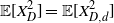 $\mathbb{E}[X_D^2]= \mathbb{E}[X_{D,d}^2]$
. Consequently, means and SCVs of the discrete case have the same bounds as the continuous case. For instance, the SCV of
 $X_{D,d}$
with
 $({\boldsymbol \pi}_D, P)$
is greater than or equal to unity.
4.3. Future research
Numerically, all continuous-time MMPP type PH-distributions have the following properties:
-
 $X_x$
is stochastically larger than
$X_{D,x}$
and
$X_x$
is stochastically larger than the exponential distribution with parameter
$\lambda = {\boldsymbol \pi}D{\bf e}$
,
-
$\operatorname{SCV}(X_x) \geq 1$
, for
$x > 0$
,
-
$\mathbb{E}[X_x]$
and
$\operatorname{SCV}(X_{D,x})$
are convex and non-increasing in x, for
$x\geq 0$
,
-
$\mathbb{E}[X_x]$
is convex in
$(d_1, d_2, \ldots, d_m)$
.



These are interesting questions for future studies.
Acknowledgements
I would like to thank two reviewers for their constructive comments and suggestions. I also want to thank Krishna Sabareesh Rajangom and Haoran Wu for proofreading the manuscript. The research was supported by an NSERC Discovery Grant.


