2.1. Tempered fractional Laplacian

Denoted by $(\varDelta +\lambda )^{\alpha } (\cdot )$, we define the tempered fractional Laplacian of the integral form as

(2.8)\begin{equation} (\varDelta+\lambda)^{\alpha} u(\boldsymbol{x}) = C_{d,\alpha} \, \mathrm{P.V.} \int_{\mathbb{R}^d }\frac{u(\boldsymbol{x})-u(\boldsymbol{s})}{\textrm{e}^{ \lambda\vert\boldsymbol{x}-\boldsymbol{s}\vert}\vert \boldsymbol{x}-\boldsymbol{s}\vert^{2\alpha+d}} \,\textrm{d}\boldsymbol{s}, \end{equation}

where $C_{d,\alpha } = ({-\varGamma ({d}/{2})}/{2 {\rm \pi}^{{d}/{2}}\varGamma (-2\alpha )}) ({1}/{{}_{2}{F}^{}_{1}(-\alpha, {(d+2\alpha -1)}/{2};{d}/{2};1)})$ for $\alpha \in (0,1)$ and $\alpha \neq \frac {1}{2}$. In particular, $d=1$ $(\varDelta +\lambda )^{\alpha }$ is reduced to the so-called Riesz fractional form, described by

(2.9)\begin{align} (\varDelta+\lambda)^{\alpha} u(x) &= ({-}1)^{\lfloor 2\alpha \rfloor +1}\frac{{}^{RL}{\mathcal{D}}_{{+}x}^{\alpha, \lambda} u(x) + {}^{RL}{\mathcal{D}}_{- x}^{\alpha, \lambda} u(x)}{2} \nonumber\\ &= C_{\alpha} \,\mathrm{P.V.} \int_{\mathbb{R} }\frac{u(x)-u(s)}{\textrm{e}^{\lambda\vert x-s\vert}\vert x-s\vert^{2\alpha+1}} \textrm{d}s, \end{align}

where $C_{\alpha } = ({-\varGamma ({1}/{2})}/{2 {\rm \pi}^{{1}/{2}}\varGamma (-2\alpha )}) ({1}/{\cos ({\rm \pi} \alpha )})$ (see Zhang et al. Reference Zhang, Deng and Karniadakis2018). In Appendix A, we detail the derivation of the Fourier transform of $(\varDelta +\lambda )^{\alpha } u(\boldsymbol {x})$, formulated as

(2.10)\begin{align} &\mathcal{F} \left[(\varDelta+\lambda)^{\alpha} u(\boldsymbol{x}) \right] (\boldsymbol{\xi}) \nonumber\\ &\quad = \mathfrak{C}_{d,\alpha} \times \left( \lambda^{2\alpha} - (\lambda^2+\xi^2)^{\alpha} {}_{2}{F}_{1}(-\alpha, \frac{d+2\alpha-1}{2};\frac{d}{2};\frac{\xi^2}{\xi^2+\lambda^2}) \right)\mathcal{F} \left[ u \right] (\boldsymbol{\xi}), \end{align}

in which $\mathfrak {C}_{d,\alpha } = {1}/{_{2}{F}^{}_{1}(-\alpha, ({d+2\alpha -1})/{2};{d}/{2};1)}$ and $\xi = \vert \boldsymbol {\xi } \vert$. For $d=3$, we define $\mathfrak {C}_{\alpha } = {1}/{{}_{2}{F}^{}_{1}(-\alpha, ({2+2\alpha })/{2};{3}/{2};1)}$. It is worth noting that when $\lambda$ approaches $0$, we recover the usual fractional Laplacian in both integral or Fourier forms.

3.1. Subgrid-scale modelling

In the description of incompressible turbulent flows, we consider LES equations (Pope Reference Pope2000), governing the dynamics of the resolved-scale flow variables,

(3.1)\begin{equation} \frac{\partial \bar{\boldsymbol{V}}}{\partial t}+ \bar{\boldsymbol{V}}\boldsymbol{\cdot} \boldsymbol{\nabla} \bar{\boldsymbol{V}}={-}\frac{1}{\rho} \, \boldsymbol{\nabla} \bar{p}+ \nu \, \boldsymbol{\nabla} \boldsymbol{\cdot} \bar{\boldsymbol{\mathsf{S}}} - \boldsymbol{\nabla} \boldsymbol{\cdot} \boldsymbol{\mathsf{T}}^{\mathcal{R}}, \end{equation}

where in the index form $\bar {\boldsymbol {V}}(\boldsymbol {x},t)=\bar {V}_i$ and $\bar {p}(\boldsymbol {x},t)$ represent the velocity and the pressure fields for $i=1,2,3$ and $\boldsymbol {x}=x_i$. Moreover, $\nu$ and $\rho$ denote the kinematic viscosity and the density, respectively. Considering $\mathcal {L}$ as the filter width, the filtered field is obtained in the form of $\bar {\boldsymbol {V}}= G \ast \boldsymbol {V}$, where $G = G(\boldsymbol {x})$ denotes the kernel of a spatial isotropic filtering type and $*$ is the convolution operator. By implementing the filtering operation, we decompose the velocity field, $\boldsymbol {V}$, into the filtered (resolved), $\boldsymbol {\bar {V}}$, and the residual, $\boldsymbol {v}$, components. In (3.1) the filtered strain rate, $\bar {\boldsymbol{\mathsf{S}}}$, and the SGS stress tensor, $\boldsymbol{\mathsf{T}}^{\mathcal {R}}$, are defined by $\bar {\boldsymbol{\mathsf{S}}}_{ij}=\frac {1}{2}({\partial V_i}/{\partial x_j}+{\partial V_j}/{\partial x_i})$ and $\boldsymbol{\mathsf{T}}^{\mathcal {R}}_{ij}=\overline {V_i V_j}-\bar {V}_i\bar {V}_j$.

Since the filtering operator cannot commute with the nonlinear terms in the NS equations, SGS stresses must be modelled in terms of the resolved velocity field. As a common yet reliable approach, Smagorinsky (Reference Smagorinsky1963) offered modelling the SGS stresses by borrowing the Boussinessq approximation from the kinetic theory such that $\boldsymbol{\mathsf{T}}^{\mathcal {R}} = -2 \nu _{R} \bar {\boldsymbol{\mathsf{S}}}$ and $\nu _{R}$ is indicated by $\nu _{R}= (C_s \mathcal {L})^2\,\vert \bar {\boldsymbol{\mathsf{S}}} \vert$, where $\vert \bar {\boldsymbol{\mathsf{S}}} \vert = \sqrt {2\bar {\boldsymbol{\mathsf{S}}}_{ij}\bar {\boldsymbol{\mathsf{S}}}_{ij}}$ and $C_s$ is the Smagorinsky (SMG) constant.

3.2. The BGK equation and the closure problem

Starting from the Boltzmann kinetic theory (Soto Reference Soto2016), the evolution of mass distribution function $f$ is governed by the BT equation as

(3.2)\begin{equation} \frac{\partial f}{\partial t} + \boldsymbol{u}\boldsymbol{\cdot} \boldsymbol{\nabla} f = \varOmega(f), \end{equation}

in which $f(t,\boldsymbol {x},\boldsymbol {u})\,\textrm {d}\boldsymbol {x}\,\textrm {d}\boldsymbol {u}$ represent the probability of finding the mass of particles, located within volume $\textrm {d}\boldsymbol {x}\,\textrm {d}\boldsymbol {u}$ centred on a specific location, $\boldsymbol {x}$, and speed, $\boldsymbol {u}$, at time $t$. It is worth noting that in the particle phase space $\boldsymbol {x}$, $\boldsymbol {u}$ and $t$ are independent variables. Technically, the left-hand side of (3.2) concerns the streaming of non-reacting particles in the absence of any body force and the right-hand side represents the collision operator. The most common form of $\varOmega (f)$ with a single collision is the so-called BGK approximation (Soto Reference Soto2016), given by

(3.3)\begin{equation} \varOmega(f)={-}\frac{f-f^{eq}}{\tau}, \end{equation}

where $\tau$ represents the single relaxation time. In the case of incompressible flows with a roughly constant temperature, $\tau$ is assumed to be independent of macroscopic flow field velocity and pressure. Moreover, under the circumstances of thermodynamic equilibrium of particles, $f^{eq}(\varDelta )$ serves as

(3.4)\begin{equation} f^{eq}(\varDelta) = \frac{\rho}{U^3}F(\varDelta), \end{equation}

where $F(\varDelta )=\textrm {e}^{-\varDelta /2}$, $\varDelta ={\vert \boldsymbol {u}-\boldsymbol {V}\vert ^2}/{U^2}$ as an isotropic Maxwellian distribution and $U$ denotes the agitation speed. More specifically, $U=\sqrt {3{k}_B T/m}$, in which ${k}_B$, $T$ and $m$ represent the Boltzmann constant, room temperature and molecular weight of air.

By recalling the basics of the BT equation from Epps & Cushman-Roisin (Reference Epps and Cushman-Roisin2018), Samiee et al. (Reference Samiee, Akhavan-Safaei and Zayernouri2020a), we introduce the following quantities: $L$ as the macroscopic length scale, $l_s$ as the microscopic characteristic length associated with the Kolmogorov length scale, $l_m$ as the average distance, travelled by a particle between successive collisions. Furthermore, we define $\boldsymbol {x}^{\prime }$ as the location of particles before scattering, where $\boldsymbol {x}$ is the current location. Thus, $\boldsymbol {x}^{\prime }=\boldsymbol {x}-(t-t^{\prime })\boldsymbol {u}$, where $\boldsymbol {u}$ is assumed to be constant during $t-t^{\prime }$. The analytical solution of (3.2) and (3.3) is given by

(3.5)\begin{align} f(t,\boldsymbol{x},\boldsymbol{u}) &= \int_{0}^{\infty} \textrm{e}^{{-}s}f^{eq}(t-s\tau,\boldsymbol{x}-s\tau \boldsymbol{u},\boldsymbol{u}) \, \textrm{d}s\nonumber\\ &=\int_{0}^{\infty} \textrm{e}^{{-}s} f^{eq}_{s,s}(\varDelta) \,\textrm{d}s, \end{align}

where $s\equiv ({t-t^{\prime }})/{\tau }$ and $f^{eq}_{s,s}(\varDelta )=f^{eq}(t-s\tau,\boldsymbol {x}-s\tau \boldsymbol {u},\boldsymbol {u})$.

In description of turbulence effects at the kinetic level, we decompose $f$ into the filtered, $\bar {f}$, and residual values, $f'$, where $\bar {f}=G*f$. As defined previously, $G$ represents the kernel of any generic spatial isotropic filtering type. Then, the filtered kinetic transport for $\bar {f}$ suffices

(3.6)\begin{equation} \frac{\partial \bar{f}}{\partial t} + \boldsymbol{u}\boldsymbol{\cdot} \boldsymbol{\nabla} \bar{f} ={-} \frac{\bar{f}-\overline{f^{eq}(\varDelta)}}{\tau}, \end{equation}

in which $u$ is independent of $t$ and $\boldsymbol {x}$. Ensuing (3.5), the analytical solution of (3.6) is described by

(3.7)\begin{equation} \bar{f} (t,\boldsymbol{x}, \boldsymbol{u}) =\int_{0}^{\infty} \textrm{e}^{{-}s} \, \overline{f^{eq}_{s,s}(\varDelta)}\, \textrm{d}s, \end{equation}

where $\overline {f^{eq}_{s,s}(\varDelta )}=\overline {f^{eq}(\varDelta (t-s\tau,\boldsymbol {x}-s\tau \boldsymbol {u},\boldsymbol {u}) )}$. Let define $\bar {\varDelta }:={\vert \boldsymbol {u}-\bar {\boldsymbol {V}} \vert ^2}/{U^2}$. Due to the nonlinear character of the collision operator (Girimaji Reference Girimaji2007), the filtering operation does not commute with $\varOmega$, which yields the following inequality as

(3.8)\begin{equation} \overline{f^{eq}(\varDelta)} = \frac{\rho}{U^3} \, \overline{\textrm{e}^{-\varDelta/2}} \neq \frac{\rho}{U^3} \, \textrm{e}^{-\bar{\varDelta}/2}=f^{eq}(\bar{\varDelta}). \end{equation}

This inequality gives rise to the so-called turbulence closure problem at the kinetic level. From the mathematical standpoint, the SGS motions stem from the convective nonlinear terms in the NS equations, which resembles the corresponding advective term of the BT equation. Therefore, it seems natural to recognize $\boldsymbol {u}\boldsymbol {\cdot } \boldsymbol {\nabla } f$ responsible for the unresolved turbulence effects in the BT equation, they manifest implicitly via the filtered collision operator though. That is, the filtered collision term on the right-hand side of (3.6) undertakes not only molecular collisions, but also the embedded SGS motions. By emphasizing on the importance of modelling $\overline {f^{eq}(\varDelta )}$ in the filtered collision operator, we review some different approaches in treating nonlinear effects.

Classical approaches. As a common practice in modelling the SGS closures, the attentions were directed toward with eddy-viscosity approximations by employing a modified relaxation time, $\tau ^{\star }$, in the BT equation (e.g. Sagaut Reference Sagaut2010). Therefore, the proposed filtered BT equation reads as

(3.9)\begin{equation} \frac{\partial \bar{f}}{\partial t} + \boldsymbol{u}\boldsymbol{\cdot} \boldsymbol{\nabla} \bar{f} ={-} \frac{\bar{f}-f^{eq}(\bar{\varDelta})}{\tau^{{\star}}}. \end{equation}

In this approach, the inequality in (3.8) is disregarded through using $\tau ^{\star }$, which renders the SGS model inappropriate for reproducing many features of the SGS motions. Nevertheless, there some non-eddy-viscosity models within the lattice Boltzmann framework, which make use of (3.8) to propose a more consistent SGS model. For more details, the reader is referred to Chen et al. (Reference Chen, Orszag, Staroselsky and Succi2004), Premnath et al. (Reference Premnath, Pattison and Banerjee2009) and Malaspinas & Sagaut (Reference Malaspinas and Sagaut2012).

Fractional approach. In the proposed framework in Samiee et al. (Reference Samiee, Akhavan-Safaei and Zayernouri2020a), the modelling of turbulence nonlinear effects begins with closing the filtered collision operator, where the multi-exponential behaviour of $\overline {f^{eq}(\varDelta )}$ is approximated properly by a heavy-tailed distribution function. Therefore, the $\overline {f^{eq}(\varDelta )}$ in (3.6) is described by

(3.10)\begin{equation} \overline{f^{eq}(\varDelta)} - f^{eq}(\bar{\varDelta}) \simeq f^{\beta}(\bar{\varDelta}), \end{equation}

where $f^{\beta }(\bar {\varDelta }) = ({\rho }/{U^3})F^{\beta }(\varDelta )$ and $F^{\beta }(\varDelta )$ denotes an isotropic Lévy $\beta$-stable distribution. By taking the first moment of (3.6), one derives the corresponding fractional Laplacian operator, termed as fractional SGS (FSGS) model, at the continuum level, where

(3.11)\begin{equation} (\boldsymbol{\nabla} \boldsymbol{\cdot} \boldsymbol{\mathsf{T}}^{R})=\mu_{\alpha} (-\varDelta)^{\alpha} \bar{\boldsymbol{V}}, \end{equation}

where $\mu _{\alpha }=({\rho (U\tau )^{2\alpha }\varGamma (2\alpha +1)}/{\tau })\,({2^{2\alpha } \varGamma (\alpha +d/2)}/{{\rm \pi} ^{d/2} \varGamma (-\alpha )})\, {c}_{\alpha }$ for $\alpha \in (0,1)$ and ${c}_{\alpha }$ is a real-valued constant. In principle, the choice of distribution function in (3.10) gives rise to a non-local operator of the resolved flow field in (3.1) as an SGS model.

Despite the notable potentials of the FSGS model in maintaining some important physical and mathematical properties of the SGS stresses, it lacks a finite second-order statistical moment. To control this statistical barrier in the FSGS model and to achieve more congruence between both sides of (3.10), we seek a finite-variance alternative for the Lévy $\beta$-stable distribution by employing the tempered counterpart and thereby a more flexible and predictive fractional operator in the LES equations in the following subsection.

3.3. Tempered fractional SGS modelling

Multi-exponential functions express a power-law behaviour in the moderate range of distribution and eventually relaxes into an exponential decay (see Evin et al. Reference Evin, Blanchet, Paquet, Garavaglia and Penot2016). By engaging more exponential terms to a multi-exponential function, the corresponding power-law behaviour extends toward long ranges; however, it is bound to vanish exponentially at the tail of the distribution, which is enforced by the nature of the physical phenomenon. As a rich class of stochastic functions for fitting into realistic phenomena, tempered stable distributions (Sabzikar et al. Reference Sabzikar, Meerschaert and Chen2015) resemble a shear power law at the moderate range and then converge to an exponential decay.

Inspired by this argument, we propose to model $\overline {f^{eq}(\varDelta )}$ with a coefficient of tempered Lévy $\beta$-stable distribution, denoted by $f^{\beta, \lambda }(\bar {\varDelta })$, within the proposed fractional framework as

(3.12)\begin{equation} \overline{f^{eq}(\varDelta)} - f^{eq}(\bar{\varDelta}) \simeq f^{Model}(\bar{\varDelta}) = {c}_{\beta,\lambda}\, f^{\beta, \lambda}(\bar{\varDelta}), \end{equation}

where ${c}_{\beta,\lambda }$ is a real-valued constant number. Moreover, we consider $\beta \in (-1-{d}/{2}, -{d}/{2})$, $\lambda >0$ and $d=3$ represents the dimension of the physical domain. Therefore, the filtered BT equation reads as

(3.13)\begin{align} \frac{\partial \bar{f}}{\partial t} + \boldsymbol{u}\boldsymbol{\cdot}\boldsymbol{\nabla} \bar{f} &={-}\frac{\bar{f}-f^{eq}(\bar{\varDelta})+f^{eq}(\bar{\varDelta})-\overline{f^{eq}(\varDelta)}}{\tau} \nonumber\\ &\simeq{-} \frac{\bar{f}-f^{eq}(\bar{\varDelta})-f^{Model}(\bar{\varDelta})}{\tau}. \end{align}

For the sake of simplicity, we take $f^{*}(\bar {\varDelta }) = f^{eq}(\bar {\varDelta })+f^{Model}(\bar {\varDelta })$. The approximation in (3.13) conceivably provides a good fit into the filtered collision operator by maintaining the significant statistical features of $\overline {f^{eq}(\varDelta )}$ and sets a physically richer starting point for developing a more expressive non-local LES model at the continuum level. It should be noted that $\beta$ and $\lambda$ rely not only on the thermodynamic properties and boundary conditions, but also they are functions of the flow Reynolds number and the filter width, $\mathcal {L}$. In following sections we assume that the Reynolds number has a relatively constant value in the stationary turbulent flow to reduce fractional parameters as a function of $\mathcal {L}$.

In this regard, the macroscopic variables associated with the flow field can be reconstructed according to

(3.14)\begin{gather} \bar{\rho} = \int_{\mathbb{R}^d} \bar{f}(t,\boldsymbol{x},\boldsymbol{u}) \,\textrm{d}\boldsymbol{u}, \end{gather}

(3.15)\begin{gather}\bar{V}_i=\frac{1}{\rho} \int_{\mathbb{R}^d} u_i \, \bar{f}(t,\boldsymbol{x},\boldsymbol{u}) \,\textrm{d}\boldsymbol{u}, \quad i=1,2,3, \end{gather}

where $\bar {\rho }=\rho$ for an incompressible flow. To establish the connection between the kinetic description and the filtered NS equation, we proceed with deriving the macroscopic form of (3.13) by multiplying it with $\boldsymbol {u}$, and integrating over the kinetic momentum, which yields

(3.16)\begin{equation} \int_{\mathbb{R}^d} \left(\boldsymbol{u} \frac{\partial \bar{f}}{\partial t} + \boldsymbol{\nabla} \boldsymbol{\cdot} (\boldsymbol{u}^2 \bar{f}) \right) \textrm{d}\boldsymbol{u} = 0 \quad \Longrightarrow \quad \rho \frac{\partial \bar{\boldsymbol{V}}}{\partial t} + \boldsymbol{\nabla} \boldsymbol{\cdot} \int_{\mathbb{R}^d} \boldsymbol{u}^2 \bar{f} \,\textrm{d}\boldsymbol{u} = 0. \end{equation}

Recalling the assumptions in remark 3.1 that $\int _{\mathbb {R}^d} \boldsymbol {u} (({\bar {f}-f^{*}(\bar {\varDelta })})/{\tau } ) \,\textrm {d}\boldsymbol {u} = 0$ due to microscopic reversibility of particle collisions. Following the derivations in Samiee et al. (Reference Samiee, Akhavan-Safaei and Zayernouri2020a, pp. 5–6), we add and subtract $\bar {\boldsymbol {V}}\bar {\boldsymbol {V}}$ to the advection term and accordingly, (3.16) is found to be

(3.17)\begin{equation} \rho \left(\frac{\partial \bar{\boldsymbol{V}}}{\partial t} + \boldsymbol{\nabla}\boldsymbol{\cdot} \bar{\boldsymbol{V}} \bar{\boldsymbol{V}} \right) ={-}\boldsymbol{\nabla}\boldsymbol{\cdot} {\varsigma}, \end{equation}

where ${\varsigma }$ in the index form is expressed as

(3.18)\begin{equation} {\varsigma}_{ij}=\int_{\mathbb{R}^d} (u_i-\bar{V}_i)(u_j-\bar{V}_j) \, \bar{f} \, \textrm{d}\boldsymbol{u}. \end{equation}

Comparing (3.1) and (3.17), it turns out that the pressure term, viscous and SGS stresses all trace back to $\boldsymbol {\nabla }\boldsymbol {\cdot } {\varsigma }$, where ${\varsigma }_{ij}=-\bar {p} \, \delta _{ij}+\boldsymbol{\mathsf{T}}^{shear}_{ij}+\boldsymbol{\mathsf{T}}^{\mathcal {R}}_{ij}$. By plugging (3.7) into the kinetic definitions of each term in ${\varsigma }_{ij}$, we obtain

(3.19)\begin{gather} \bar{p} \, \delta_{ij} ={-}\int_{\mathbb{R}^d} (u_i-\bar{V}_i)(u_j-\bar{V}_j) \, f^{*}(\bar{\varDelta}) \, \textrm{d}\boldsymbol{u} \int_{0}^{\infty} \textrm{e}^{{-}s} \,\textrm{d}s, \end{gather}

(3.20)\begin{gather}\boldsymbol{\mathsf{T}}_{ij}^{shear} = \int_{0}^{\infty} \int_{\mathbb{R}^d} (u_i-\bar{V}_i)(u_j-\bar{V}_j) \times \left(f^{eq}_{s,s}(\bar{\varDelta})-f^{eq}(\bar{\varDelta})\right) \textrm{e}^{{-}s} \,\textrm{d}\boldsymbol{u}\, \textrm{d}s = 2 \mu \bar{\boldsymbol{\mathsf{S}}}_{ij}, \end{gather}

where $\mu =\rho U^2\tau$. Similarly, by employing $f^{Model}$ in (3.12), we attain

(3.21)\begin{align} \boldsymbol{\mathsf{T}}_{ij}^{R} &={c}_{\beta,\lambda}\, \int_{0}^{\infty} \int_{\mathbb{R}^d} (u_i-\bar{V}_i)(u_j-\bar{V}_j) \left(f^{\beta,\lambda}_{s,s}(\bar{\varDelta})-f^{\beta,\lambda}(\bar{\varDelta})\right) \textrm{e}^{{-}s} \,\textrm{d}\boldsymbol{u}\, \textrm{d}s \nonumber\\ &=\frac{\rho {c}_{\beta,\lambda}}{U^3} \int_{0}^{\infty} \int_{\mathbb{R}^d} (u_i-\bar{V}_i)(u_j-\bar{V}_j) \left(F^{\beta,\lambda}(\bar{\varDelta}_{s,s})-F^{\beta,\lambda}(\bar{\varDelta})\right) \textrm{e}^{{-}s} \,\textrm{d}\boldsymbol{u}\, \textrm{d}s, \end{align}

in which $\bar {\varDelta }_{s,s} = \bar {\varDelta }(t-s\tau,\boldsymbol {x}-s\tau \boldsymbol {u}, \boldsymbol {u})$. As discussed in Samiee et al. (Reference Samiee, Akhavan-Safaei and Zayernouri2020a, appendix), the temporal shift can be detached from $f^{\beta,\lambda }_{s,s}(\bar {\varDelta })$ and then $\bar {\varDelta }_{s,s}$ is simplified to $\bar {\varDelta }_s = \bar {\varDelta }(t,\boldsymbol {x}-s\tau \boldsymbol {u}, \boldsymbol {u})$. Therefore,

(3.22)\begin{equation} \boldsymbol{\mathsf{T}}_{ij}^{R} = \frac{\rho {c}_{\beta,\lambda}}{U^3} \int_{0}^{\infty} \int_{\mathbb{R}^d} (u_i-\bar{V}_i)(u_j-\bar{V}_j) \left(F^{\beta,\lambda}(\bar{\varDelta}_{s})-F^{\beta,\lambda}(\bar{\varDelta})\right) \textrm{e}^{{-}s} \,\textrm{d}\boldsymbol{u}\, \textrm{d}s. \end{equation}

The strategy to evaluate $\boldsymbol{\mathsf{T}}_{ij}^{R}$ is to decouple the particle speed into time and displacement by employing $\boldsymbol {u}=({\boldsymbol {x}^{\prime }-\boldsymbol {x}})/{s\tau }$ and approximate the asymptotic behaviour of $F^{\beta,\lambda }(\bar {\varDelta })$ with a tempered power-law distribution. In a detailed discussion in Appendix B, we show that

(3.23)\begin{equation} \boldsymbol{\mathsf{T}}_{ij}^{R} = {c}_{\alpha,\lambda} \, \bar{\nu}_{\alpha} \sum_{k=0}^{\mathcal{K}} \bar{\phi}_{k}^{\mathcal{K}}(\alpha) \int_{\mathbb{R}^d} (x_i -x_i^{\prime}) \, (x_j -x_j^{\prime}) \frac{(\boldsymbol{x} -\boldsymbol{x}^{\prime})\boldsymbol{\cdot} (\bar{\boldsymbol{V}}- \bar{\boldsymbol{V}}^{\prime} ) }{\vert \boldsymbol{x} -\boldsymbol{x}^{\prime}\vert^{2\alpha+5} \, \textrm{e}^{\bar{\lambda}_k \vert \boldsymbol{x} -\boldsymbol{x}^{\prime} \vert}} \textrm{d}\kern0.06em\boldsymbol{x}^{\prime}, \end{equation}

in which $\bar {\nu }_{\alpha } = (2\alpha +3) (\rho C_{\alpha } \tau ^{2\alpha -1} U^{2\alpha })$ for $\alpha \in (0,\frac {1}{2})\cup (\frac {1}{2},1)$ and recalling $\bar {\lambda }_k = ({k}/{\tau U})\lambda$. Moreover, $\bar {\phi }_{k}^{\mathcal {K}}(\alpha )$ is indicated in (B9). Eventually, we disclose the integral form of $\boldsymbol {\nabla }\boldsymbol {\cdot } \boldsymbol{\mathsf{T}}^{\mathcal {R}}$ as

(3.24)\begin{equation} (\boldsymbol{\nabla}\boldsymbol{\cdot} \boldsymbol{\mathsf{T}}^{\mathcal{R}})_j = {c}_{\alpha,\lambda} \, \bar{\nu}_{\alpha} \sum_{k=0}^{\mathcal{K}} \frac{(2\alpha+\bar{\lambda}_k)}{(2\alpha+3)} \bar{\phi}_{k}^{\mathcal{K}}(\alpha) \int_{\mathbb{R}^d} \frac{(\bar{V}_j -\bar{V}_j^{\prime}) }{\vert \boldsymbol{x} -\boldsymbol{x}^{\prime}\vert^{2\alpha+3} \, \textrm{e}^{\bar{\lambda}_k \vert \boldsymbol{x} -\boldsymbol{x}^{\prime} \vert}} \textrm{d}\kern0.06em\boldsymbol{x}^{\prime}, \end{equation}

where $\nu _{\alpha } = {c}_{\alpha,\lambda } \bar {\nu }_{\alpha }$. Recalling the integral representation of a tempered fractional Laplacian in (2.8), we formulate the divergence of the SGS stresses as

(3.25)\begin{equation} (\boldsymbol{\nabla}\boldsymbol{\cdot} \boldsymbol{\mathsf{T}}^{\mathcal{R}})_j = \nu_{\alpha} \sum_{k=0}^{\mathcal{K}} \phi_{k}^{\mathcal{K}}(\alpha,\lambda) (\varDelta+\bar{\lambda}_k)^{\alpha} \bar{V}_j, \end{equation}

where $\phi _{k}^{\mathcal {K}}(\alpha,\lambda ) = ({(2\alpha +\bar {\lambda }_k)}/{(2\alpha +3)})\bar {\phi }_{k}^{\mathcal {K}}(\alpha )$. Evidently, by setting $\mathcal {K} = 0$, we find that $\bar {\phi }_{k}^{\mathcal {K}}(\alpha )=\varGamma (2\alpha )$ and the new operator in (3.25) reduces to a fractional Laplacian, which recovers the FSGS model.

Inferring from (3.25), our choice in the kinetic description of turbulent effects reflects in the form of a tempered fractional operator through a rigorous connection between the filtered BT and the filtered NS equations. More specifically, we adopt $\mathcal {K} = 1$ and, hence, the TFSGS model can be formulated as

(3.26)\begin{equation} \boldsymbol{\nabla}\boldsymbol{\cdot} \boldsymbol{\mathsf{T}}^{\mathcal{R}} = \nu_{\alpha} \left[ \phi_{0}^{1}(\alpha)\left(- (-\varDelta)^{\alpha} \right) \bar{\boldsymbol{V}} + \phi_{1}^{1}(\alpha)\left(\varDelta+\bar{\lambda}_1 \right)^{\alpha} \bar{\boldsymbol{V}} \right], \end{equation}

where $\phi _{0}^{1}(\alpha ) = ({1}/{(2\alpha +3)}) ( \varGamma (2\alpha +1)-\varGamma (2\alpha ) )$ and $\phi _{1}^{1}(\alpha,\lambda ) = ({(2\alpha +\lambda )}/{(2\alpha +3)} ) \varGamma (2\alpha -1)$. Accordingly, the governing LES equations read as

(3.27)\begin{equation} \frac{\partial \bar{V}_i}{\partial t}+\frac{\partial \bar{V}_i\,\bar{V}_j}{\partial x_j}={-}\frac{1}{\rho}\frac{\partial \bar{p}}{\partial x_i}+\nu \, \varDelta \bar{V}_i -\nu_{\alpha} \sum_{k=0}^{1} \phi_{k}^{1}(\alpha,\lambda) (\varDelta+\bar{\lambda}_k)^{\alpha} \, \bar{V}_i, \end{equation}

where $\alpha \in (0,\frac {1}{2})\cup (\frac {1}{2},1)$, $\lambda >0$ and $\nu _{\alpha } = {\mu _{\alpha }}/{\rho }$.

3.4. TFSGS formulations for the SGS stresses

To study the key role of tempering fractional operators in recovering turbulent statistical structures, it is essential to establish a straightforward form of the modelled SGS stresses. Due to some numerical complications in evaluating the integral in (3.24), we settle to proceed with the Fourier representation of the TFSGS model. Employing the definition of $\mathcal {I}^{\alpha }$ ($\alpha$-Riesz potential) from Stein (Reference Stein1970), it is possible to verify that

(3.28)\begin{equation} \boldsymbol{\nabla}\boldsymbol{\cdot} \boldsymbol{\mathsf{T}}^R = (\varDelta+\lambda)^{\alpha} \boldsymbol{\bar{V}} = \boldsymbol{\nabla\cdot\nabla} \mathcal{I}^{\alpha = 1}\left[ \nu_{\alpha} \sum_{k=0}^{1} \phi_{k}^{1}(\alpha,\lambda) (\varDelta+\bar{\lambda}_k)^{\alpha} \boldsymbol{\bar{V}} \right]. \end{equation}

Inspired by (3.28), we introduce $\mathcal {R}_j^{\alpha,\lambda } (\boldsymbol {\cdot }) = \boldsymbol {\nabla }_j \mathcal {I}^{\alpha =1} (\varDelta +\lambda )^{\alpha } (\boldsymbol {\cdot })$ as a tempered fractional operator such that

(3.29)\begin{equation} \boldsymbol{\mathsf{T}}^R_{ij} = \frac{\nu_{\alpha}}{2}\sum_{k=0}^{1} \phi_{k}^{1}(\alpha,\lambda) \left[ \mathcal{R}_j^{\alpha,\bar{\lambda}_k} \bar{V}_i + \mathcal{R}_i^{\alpha,\bar{\lambda}_k} \bar{V}_j \right], \end{equation}

where $\mathcal {F} [ I^{\alpha =1} ] = {1}/{\xi ^2}$ and $\mathcal {F} [ \boldsymbol {\nabla }_j ] (\boldsymbol {\xi }) = - \mathfrak {i} \, \xi _j$ and $\mathfrak {i}$ denotes an imaginary unite. Following (2.10) into (3.29), we find the Fourier form of $\mathcal {R}_j^{\alpha,\lambda }$ as

(3.30)\begin{equation} \mathcal{F} \left[ \mathcal{R}_j^{\alpha,\lambda} \right] (\boldsymbol{\xi}) = \mathfrak{C}_{\alpha} \frac{ - \mathfrak{i} \, \xi_j}{\xi^2} \left( \lambda^{2\alpha} - (\lambda^2+\xi^2)^{\alpha} \,{}_{2}{F}^{}_{1}\left(-\alpha, 1+\alpha;\frac{3}{2};\frac{\xi^2}{\xi^2+\lambda^2}\right) \right). \end{equation}

4.1. Optimization strategy

Devising a robust optimization framework is an inevitable element in predictive fractional and tempered fractional modellings (see Burkovska et al. Reference Burkovska, Glusa and D'Elia2020; Pang et al. Reference Pang, D'Elia, Parks and Karniadakis2020). Regarding the given set of conditions for the closure problem, we find conditions (a) and (c) practically crucial in developing an approach for estimating the parameters and coefficient associated with the TFSGS model while condition (b) can be substantially recovered by imposing (4.2), where $G_{LLL}(r,t)\vert _{r=0}=\langle \bar {V}_i \boldsymbol{\mathsf{T}}^{R}_{ij}\rangle$. As we learn from the one-point correlation analysis in Samiee et al. (Reference Samiee, Akhavan-Safaei and Zayernouri2020a) and the following section, correlations between the SGS stresses, obtained by the DNS data and the model, highly rely on $\alpha$ and $\lambda$ in the TFSGS model rather than playing a central role in capturing the SGS dissipation energy and non-local structure functions. This approach provides the basis for an optimal estimation of the fractional exponents ($\alpha$ and $\lambda$) by employing the normalized $D_{LL}$ and $\varrho _{i}$, defined in algorithm .

Algorithm 1

Estimation of the optimal model parameters for a specific $\mathcal {L}$

By fixing the values of fractional exponents, it is possible to accurately quantify the model coefficient and thereby reproduce the third-order structure in (4.2) via modelling $G_{LLL}$. In algorithm  we schematically present the proposed method for optimizing the parameters associated with the TFSGS model at a given flow Reynolds number (Re) and a specific filter width, $\mathcal {L}$.

It must be noted that in step 3, we define

(4.4)\begin{equation} \boldsymbol{\mathsf{T}}^{R,N}_{ij}= \frac{\boldsymbol{\mathsf{T}}^{R,TF}_{ij}}{\mathrm{c}_{\alpha,\lambda} }=\frac{\bar{\nu}_{\alpha}}{2}\sum_{k=0}^{1} \phi_{k}^{1}(\alpha,\lambda) \left[ \mathcal{R}_j^{\alpha,\bar{\lambda}_k} \bar{V}_i + \mathcal{R}_i^{\alpha,\bar{\lambda}_k} \bar{V}_j \right]. \end{equation}

Moreover, superscripts ‘$D$’ and ‘$TF$’ represent the values obtained by filtering the true DNS data and the TFSGS model, respectively.

5.1. Direct numerical simulation database and LES platform

In terms of a priori tests, we conduct the numerical simulation of a forced HIT flow employing the open-source pseudo-spectral NS solver for a triply periodic domain, the code of which is presented at Akhavan-Safaei & Zayernouri (Reference Akhavan-Safaei and Zayernouri2020) and the references therein (e.g. Mortensen & Langtangen Reference Mortensen and Langtangen2016). It should be noted that in the next section, the LES solver is successfully prepared using this DNS code and the statistically stationary DNS dataset presented here is filtered and used as the initial conditions for the final a posteriori assessments.

Using the NS solver, we performed DNS of a stationary HIT flow with $320^3$ resolution for a periodic computation domain as $\varOmega =[0,2{\rm \pi} ]^3$ and the large-scale forcing occurs at $0 < \vert \boldsymbol {\xi } \vert \leqslant 2$ to maintain turbulence statistics stationary. Here, $\boldsymbol {\xi }$ represents the vector of Fourier wave numbers and $\xi _{max}=\sqrt {2}\,N/3$ is the maximum wave number solved numerically, where $N=320$ is the number of grid points. In this case, $\xi _{max}\,\eta _{k}=1.6>1$ certifies that all the scales of motion are well resolved, where $\eta _{k}$ refers to the Kolmogorov length scale. We detail the flow parameters and some of the statistical properties in table 1, in which $\varepsilon$ and $E_{tot}$ denote the expected values of dissipation rate and turbulent kinetic energy, respectively. Moreover, $Re_{\lambda }=\frac {u^\prime _{rms} \, l_{\lambda }}{\nu }$ and $l_{\lambda }=\sqrt {15 \nu \, {u'}_{rms}^2/\varepsilon }$ represent the Taylor Reynolds number and micro-scale length, respectively, where $u'_{rms}=\sqrt {2E_{tot}/3}$. The simulation undergoes running for $30$ eddy turnover times, $\tau _{\mathscr {L}}$, to construct $40$ sample snapshots as our database. Due to the present homogeneity and isotropy in the HIT flow, we find the database adequate for obtaining the required statistics in the further analysis. The kurtosis and skewness values of the diagonal components of velocity gradient tensor are also presented in table 1, supporting non-Gaussianity of turbulent structures.

Table 1.

Flow parameters and statistical properties in the DNS of a forced HIT flow.

For the purpose of crunching a heavy DNS database in the statistical analysis, we develop an LES platform in Python with a focus on efficiency in obtaining two-point correlations and the ease of dealing with the fractional operators. This platform consists of three chief components: filtering the DNS database, implementation of LES models and optimization, and executing the final analysis. To overcome the burden of a timely filtering process especially in two-point correlation analysis, we introduce the scalable multi-threaded filtering code using Numpy, threading and astropy.convolution packages. Further steps in finding the optimum model parameters and applying the Fourier form of the fractional models are developed by employing the highly efficient Intel® MKL library. For more information, the reader is referred to Samiee (Reference Samiee2021).

5.2. Optimal estimation of fractional parameters

In order to optimize the efficiency of the TFSGS model, we developed a flexible and rigorous strategy in algorithm . The proposed algorithm is equipped with verification and validation mechanisms through the conventional correlation coefficients and two-point structure functions. Recalling from § 4.1 that $\boldsymbol{\mathsf{T}}^{R,D}_{ij}$ denotes the true SGS stresses obtained by filtering the well-resolved DNS data. Moreover, $\boldsymbol{\mathsf{T}}^{R,*}_{ij}$ represents the general form of modelled SGS values, where $*$ can be replaced by $TF$ or $SM$ in the TFSGS or SMG models, respectively.

The first step in algorithm  concerns detecting the optimum value of the fractional exponent, $\alpha ^{opt}$, where the maximum of ensemble-averaged correlation between $\boldsymbol{\mathsf{T}}^{R,D}_{ii}$ and $\boldsymbol{\mathsf{T}}^{R,TF}_{ii}$, denoted by $\varrho _{ii}$, occurs. Endorsed by the results of table 2, the tempering parameter, $\lambda$, appears not to make any noticeable change in $\varrho _{ii}$, namely less than 3%. Therefore, we plot the variations of $\varrho _{ii}$ vs $\alpha ^{opt}$ in figure 1 for $i=1,2,3$ in the absence of $\lambda$, where each dashed box specifies the interval of $\alpha$ yielding the maximum of $\varrho _{ii}$. Without any loss of accuracy, we adopt $\alpha ^{opt}=0.76$, 0.58, 0.51 as the corresponding minimum value in each specified interval for $\mathcal {L}_{\delta }= {\mathcal {L}}/{2 \delta x}=4,\,8,\,12$, respectively, where $\delta x={2{\rm \pi} }/{N}$ represents the computational grid size.

Figure 1.

Variation of the correlation coefficients (a) $\varrho _{11}$, (b) $\varrho _{22}$ and (c) $\varrho _{33}$ vs $\alpha \in (0,1)$ for $\mathcal {L}_{\delta }=4,\,8,\,12$ by setting $\lambda \simeq 0$ in (4.4). The maximum values lie in the dashed boxes.

Table 2.

The ensemble-averaged correlation coefficients ($\varrho _{ii}$) between SGS stresses obtained by the filtered DNS data ($\boldsymbol{\mathsf{T}}^{R,D}_{ii}$) and the TFSGS model ($\boldsymbol{\mathsf{T}}^{R,TF}_{ii}$) for $i=1,2,3$. In the fractional models, $\alpha ^{opt}$ is set as $0.76$, $0.58$ and $0.51$ for $\mathcal {L}_{\delta }=4,\,8,\,12,$ respectively.

From the kinetic perspective, enlarging $\mathcal {L}_{\delta }$, $\overline {f^{eq}(\varDelta )}$ in (3.6) demonstrates an increasingly multi-exponential pattern, which can be better described by a power-law distribution function. This argument accounts for the prediction enhancement in figure 1, achieved by the TFSGS model and the abduct reduction of $\alpha ^{opt}$ vs $\mathcal {L}_{\delta }$ (see Samiee et al. Reference Samiee, Akhavan-Safaei and Zayernouri2020a, p. 10). Theoretically, the tempered power-law distribution can resemble a power-law or a Gaussian distribution by letting $\lambda$ go to $0$ or $\infty$, respectively. This allows the TFSGS model to span the gap between the FSGS model, representing self-similar behaviour of the inertial range, and the SMG model, renowned for its dissipative characteristics. The results in table 2 support this line of reasoning by a row of correlation quantities for the given filter widths, particularly at $\mathcal {L}_{\delta }=12$.

On this background, we proceed with the second step in algorithm  to indicate $\lambda ^{opt}$ through a comparative study of the normalized stress–strain correlation function, defined as $S_{\varDelta } = {D_{LL}(r,t)}/{D_{LL}(0,t)}$. With the knowledge of $D_{LL}(r,t)$, we extend the two-point correlation analysis to the spectral space by evaluating the instantaneous radial dissipation spectrum, given by $\hat {\mathcal {D}}(\xi )=\mathcal {F} {[}D_{LL}(r,t) {]}(\xi )$. To evaluate the error between the dissipation spectrum, obtained by the true DNS data and the LES models at high wave numbers, we define

(5.1)\begin{equation} \mathcal{E}_{H} = \frac{\left\vert \left[ \hat{\mathcal{D}}(\xi)\right]^{*} - \left[\hat{\mathcal{D}}(\xi)\right]^{D}\right\vert}{\left\vert \left[ \hat{\mathcal{D}}(\xi)\right]^{D} \right\vert}, \end{equation}

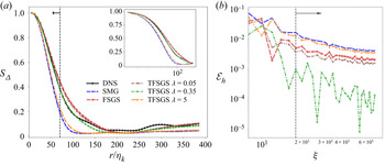
where ${\vert } \cdot {\vert }$ represents the norm of the vector. Figure 2(a) displays $S_{\varDelta }$ vs the spatial shift, $r$, for a logarithmic sequence of $\lambda$ spanning three orders of magnitude in the TFSGS model, where $\mathcal {L}_{\delta }=8$. As stated earlier, the proposed model can take a journey from the FSGS to the SMG models by tuning $\lambda$. Evidently, the true quantities of $S_{\varDelta }$, coloured black, are well predicted by the proposed model with $\lambda ^{opt}=0.45$, where $\alpha ^{opt}=0.58$ is fixed. Figure 2(b) confirms our findings quantitatively in a plot of $\mathcal {E}_{H}$ vs radius of wave numbers, $\xi$, with log-scale axes. In fact, this plot implies accuracy of the TFSGS model in capturing the two-point structure function at the dissipation range, as pointed by an arrow.

Figure 2.

(a) Comparing results of the normalized two-point stress–strain rate correlation functions ($S_{\varDelta }$) and (b) error analysis of the longitudinal dissipation spectrum ($\mathcal {E}_{H}$) for FSGS and SMG models, where $\mathcal {L}_{\delta }=8$ and $\xi$ represents the radius of Fourier wave numbers. In both plots, the arrows point to the dissipation range.

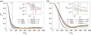
Employing the same analysis for $\mathcal {L}_{\delta }=4, \, 12,$ we infer the optimal behaviour of the TFSGS model, evaluated for a logarithmic range of $\lambda$ with a fixed $\alpha ^{opt}$, in figure 3. The inset plots show $\mathcal {E}_{H}$ vs $\xi$ using log-scale on both axes to magnify the dissipation range at high wave numbers. Interestingly, at $\mathcal {L}_{\delta }=4$ the FSGS model is dissipative enough to outperform the tempered model in capturing the true $S_{\varDelta }$ in figure 3(a). With all this in mind, these results certify the importance of tempering in correct regeneration of two-point correlation functions particularly at larger filter widths ($\mathcal {L}_{\delta }=8, \, 12$). Moreover, the SMG model, resembling the TFSGS with $\lambda \sim 5$, exhibits a relatively steeper slope at the dissipation range, which is rooted in the diffusive form of its operator. In this context, tempering plays a crucial role in characterizing dissipation structures covering the widening gaps between the asymptotic cases ($\lambda = 0.01$ and $5$) in figure 3(b). This brings up the TFSGS model as a superior physics-based model in comparison with its counterparts, i.e. the SMG and FSGS models.

Figure 3.

Comparing results of the normalized two-point stress–strain rate correlation functions for (a) $\mathcal {L}_{\delta }=4$ and (b) $\mathcal {L}_{\delta }=12$. The inset plots illustrate the normalized error of longitudinal dissipation spectrum ($\mathcal {E}_{H}$) vs the radius of Fourier wave numbers ($\xi$). The arrows point to the dissipation range.

Given the values of $\alpha ^{opt}$ and $\lambda ^{opt}$, we proceed lastly with quantifying ${c}_{\alpha,\lambda }$ as prescribed in algorithm . Under statistically stationary circumstances of the flow field, ${c}_{\alpha,\lambda }$ remains fairly unchanged for each $\mathcal {L}_{\delta }$ of interest, as reported in table 3. It should be noted that ${c}_{\alpha,\lambda }$ is part of the fractional coefficient, described in (4.4), to scale up the model in a constant $Re_{\lambda }$ and $\mathcal {L}_{\delta }$.

Table 3.

Optimized parameters associated with the TFSGS model in terms of algorithm  for differing filter widths.

5.3. Interpretation of two-point structure functions

The third-order structure functions, arising from the KH equations, provide insights about the statistics of unresolved scales and their strong interactions with large-scale motions. As discussed previously in § 4, $G_{\varDelta } = {G_{LLL}}/{\epsilon \mathcal {L}}$, representing the scaled two-point velocity-stress correlation function, is introduced as a sufficient condition for precise regeneration of third-order structure functions and an a priori consistency in LES modelling. Following the derivation of the longitudinal Taylor macroscale in Pope (Reference Pope2000, chap. 6), $D_{LL}(r)$ seems to be directly connected to the first-order derivative of $G_{LLL}(r)$ at the dissipation range. This offers the capability of the optimum edition of the TFSGS model in capturing $G_{\varDelta }$ and thereby fulfilling the essential conditions in (4.2).

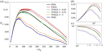
In the first stage of the statistical analysis, we perform a comprehensive study on $G_{\varDelta }$ in figure 4(a) for $\mathcal {L}_{\delta } = 8$, in which the dissipation and inertial ranges are magnified in figure 4(b) with a semi-logarithmic scale on the $x$-axis and figure 4(c) with logarithmic scales on both axes, respectively. The balance regions (BR), including extremum points, are thickened up in all the graphs in figure 4(a). Balance regions also indicate the transitional zone between dissipation and inertial ranges. Aligned with the right side of (4.2), the trend of $G_{\varDelta }$ at small-scale interactions appear to be a linear function of spatial displacement, $r$, suggested by Meneveau (Reference Meneveau1994, figure 2). The results in figure 4(a) and more accurately in figure 4(b) offer that the optimum TFSGS model well predicts the true DNS quantities at the left side of the BR, not only the slope of $G_{\varDelta }$ but also the maximum of $G_{\varDelta }$ occurring at a relatively close $r$. This spotlights the importance of step three of algorithm  in tuning the slope of $G_{\varDelta }$ at the dissipation range and the effective role of the tempering parameter in fitting the BR, associated with the filtered DNS data. 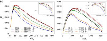In practice, increasing $\lambda$ pushes the BR toward the left side to preserve the increasing linear correlation as a notion of more dissipative behaviour. These findings are endorsed qualitatively for the other filter widths in figure 5, considering $\lambda ^{opt}$ in table 3.

Figure 4.

Two-point velocity-stress correlation function in a stationary HIT flow for $\mathcal {L}_{\delta }=8$ using box filtering. The segment of the balance region (BR) has been thickened up in (a) for all the graphs. The dissipation and the inertial ranges have been enlarged in plots (b) with semi-logarithmic scale on the $x$-axis and (c) with a logarithmic scale on both axes, respectively.

Figure 5.

Two-point velocity-stress correlation function in a stationary HIT flow for (a) $\mathcal {L}_{\delta }=4$ and (b) $\mathcal {L}_{\delta }=12$ using box filtering. The inertial range has been enlarged in the inset plots with a logarithmic scale on both axes.

In analysis of $G_{\varDelta }$ at the inertial range, the graph, associated with $\lambda ^{opt}$, shows a favourable match with true points, coloured black, in figures 4 and 5. For the purpose of clarity, the inertial ranges are magnified in log-log scale plots in figure 4(c) for $\mathcal {L}_{\delta }=8$ and the inset plots in figure 5 for $\mathcal {L}_{\delta }=4, \, 12$, respectively. Motivated by these results, tempered fractional modelling seems to be faithful in fitting structures at the dissipation and the inertial ranges and also estimating the correct value of $r$, associated with the extremum points. Inevitably, enlarging $\mathcal {L}_{\delta }$ accounts for inaccuracies in fitting the tail of graphs as observed in 5(b). Notwithstanding, the mid-range interactions are acceptably predicted by the optimized TFSGS model.

With an overview of the present results, the TFSGS model stands out as a structure-based approach, which reasonably covers the gap between the FSGS and SMG models. In $\mathcal {L}_{\delta }=4$, $\lambda ^{opt}$ is found to be very close to zero, which renders tempering non-essential in capturing two-point structures. As we increase $\mathcal {L}_{\delta }$, this gap starts widening up and the tempering mechanism acts more dynamically in finding the true BR and fitting the dissipation structures. This argument confirms that the tempered fractional approach displays great potential for parameterizing structure function especially at larger filter widths while retaining fairly acceptable accuracy.

5.4. Probability density function of SGS stresses

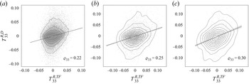
Within the proposed statistical framework, the last step in algorithm  focuses on the probability density functions (PDFs) of filtered DNS data. The key idea is to assess the performance of models and verify if the proposed model maintains the true statistics. In this context, we present the scatter plots of $\boldsymbol{\mathsf{T}}^{R,D}_{ii}$ against $\boldsymbol{\mathsf{T}}^{R,TF}_{ii}$ in figure 6 for three given filter widths and $i=3$. We should note that the present results are confined to $i=3$ due to the similarities in other directions. The slope in each plot is indicated by the corresponding correlation coefficients in table 2. The most noticeable specific about these results is that the data points are bounded within a same order of magnitude on both axes. 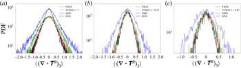As a matter of fact, we achieve a roughly unit regression coefficient between $\boldsymbol{\mathsf{T}}^{R,D}_{ii}$ and $\boldsymbol{\mathsf{T}}^{R,TF}_{ii}$, where our optimization strategy targets for correct estimation of the SGS dissipation. This analysis can be extended to the PDF plots in figure 7. With nearly the same correlation coefficients, the SMG model fails to reproduce the true statistics, while the optimum TFSGS model offers a great match with the true graphs. As pointed out previously, in $\mathcal {L}_{\delta }=4$ the FSGS model represents the equivalent form of the TFSGS with $\alpha ^{opt}=0.76$ and $\lambda ^{opt}\simeq 0$.

Figure 6.

Scatter plots of the SGS stresses obtained by the filtered DNS data ($\boldsymbol{\mathsf{T}}^{R,D}_{33}$) vs the modelled stresses ($\boldsymbol{\mathsf{T}}^{R,TF}_{33}$) using optimized parameters in table 3 for (a) $\mathcal {L}_{\delta }=4$, (b) $\mathcal {L}_{\delta }=8$ and (c) $\mathcal {L}_{\delta }=12$.

Figure 7.

Probability density function of the ensemble-averaged $( \boldsymbol {\nabla } \boldsymbol {\cdot } \boldsymbol{\mathsf{T}} )_{i=3}$ for the optimized (tempered) fractional and the SMG models at (a) $\mathcal {L}_{\delta }=4$, (b) $\mathcal {L}_{\delta }=8$ and (c) $\mathcal {L}_{\delta }=12$.

From the understanding of energy cascading in turbulent flows, the SGS dissipation, $\epsilon$, is considered as an external parameter in two-point structure equations for describing small-scale motions. In the statistical sense, we compare the PDFs of $\epsilon$, implied by the models, with the true PDFs, obtained by the filtered DNS data for $\mathcal {L}_{\delta }=4$, 8, 12. As shown in figure 8, the fractional models accurately predict the forward scattering, associated with the positive dissipation, $\epsilon ^{+}$, while the SMG model appears to be too dissipative due to its positive eddy viscosity. Furthermore, the TFSGS model presents an underprediction of the backward scattering by producing a slim amount of negative dissipation, $\epsilon ^{-}$. On the side of numerical analysis, this limitation results in preserving numerical stability by minimizing negative dissipation error.

Figure 8.

Probability density function of the ensemble-averaged SGS dissipation for the optimized (tempered) fractional and the SMG models at (a) $\mathcal {L}_{\delta }=4$, (b) $\mathcal {L}_{\delta }=8$ and (c) $\mathcal {L}_{\delta }=12$.

5.5. A posteriori analysis

With a focus on numerical stability, we extend the statistical a priori assessments to an a posteriori analysis in order to evaluate performance of the proposed models in time. We employ the pseudo-spectral solver, described in § 5.1, on $\varOmega$ discretized with a uniform grid of $520^3$ resolution, and resolve over $5$ eddy turnover times, $\tau _{\mathscr {L}}$, to provide the DNS flow fields. The simulation is initiated with an instantaneous flow field, obtained from the sufficiently resolved DNS of a stationary HIT flow at $Re_{\lambda } = 240$. The comprehensive characteristics of this fully developed turbulent field are reported in Akhavan-Safaei & Zayernouri (Reference Akhavan-Safaei and Zayernouri2020). By the explicit filtering of this initial flow field, the a posteriori simulations are carried out on $130^3$ and $52^3$ grids for the corresponding $\mathcal {L}_{\delta }=2$, $5$, respectively.

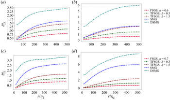
This analysis allows for structural comparisons between the fractional models and the filtered DNS data through tracking the evolution of resolved turbulent kinetic energy, $K_{tot}(t) = \langle {\bar {V}_i\bar {V}_i}/{2}\rangle _s$. Figure 9 displays the decay of the resolved kinetic energy, which verifies computational stability of the fractional models. The TFSGS models associated with $\alpha =0.7$ and $\lambda =0.3$ for $\mathcal {L}_{\delta }=2$, and $\alpha =0.6$ and $\lambda =0.5$ for $\mathcal {L}_{\delta }=5$ present a favourable match with the true decaying of $K_{tot}$ compared with the SMG and dynamic SMG models. These results spotlight the importance of tempering in the correct prediction of kinetic energy while by increasing $\lambda$, the TFSGS model asymptotes overpredictions of the SMG model for both $\mathcal {L}_{\delta }=2$, $5$.

Figure 9.

Decay of the resolved turbulent kinetic energy, $K_{tot}$, for the optimized TFSGS and the SMG models with (a) $52^3$ and (b) $130^3$ grid points.

Given the a priori analysis in previous subsections, the model parameters are fitted through satisfying both sides of (4.2), which are inherently connected with the second- and third-order structure functions. In figure 10 we study the two-point second-order structure functions, ${B}_{LL}$, after $2$ and $4$ eddy turnover times of simulation. It should be noted that ${B}_{LL}^{n}$ and ${B}_{LLL}^{n}$ represent the second- and third-order correlation functions from the LES models, which are normalized by the corresponding filtered DNS solutions, respectively. Supported by the results in figure 10, the TFSGS model, associated with the optimum $\lambda$, maintains ${B}_{LL}$ over a wide range of $r$ although presenting small inconsistencies at small scales. As an essential condition to a physically accurate SGS model, the optimized TFSGS also provides a fairly accurate and reliable prediction of ${B}_{LLL}$ compared with the FSGS and the eddy-viscosity approaches in figure 11. In this vein, we also present the energy spectra, $E_{\xi }$, resulting from the LES for different values of $\lambda$ in figure 12 and compare it with the corresponding $E_{\xi }$ from the DNS results at $t=2\tau _{\mathcal {L}}$ and $4\tau _{\mathcal {L}}$.

Figure 10.

Two-point second-order structure functions of the resolved velocity fields normalized by the filtered DNS data for (a,b) $\mathcal {L}_{\delta }=5$ and (c,d) $\mathcal {L}_{\delta }=2$ at $t=2\tau _{\mathscr {L}}$ and $t=4\tau _{\mathscr {L}}$, respectively.

Figure 11.

Third-order structure functions of the resolved velocity fields normalized by the filtered DNS data for (a) $\mathcal {L}_{\delta }=5$ and (b) $\mathcal {L}_{\delta }=2$ at $t=4\tau _{\mathscr {L}}$.

Figure 12.

Energy spectra ($E_{\xi }$) vs $\xi$, resulting from $130^3$ LES cases with the TFSGS models evaluated for $\alpha =0.7$ and $\lambda =0$, 0.3, 1.5 for $\mathcal {L}_{\delta }=2$ at (a) $t=2\tau _{\mathscr {L}}$ and (b) $t=4\tau _{\mathscr {L}}$.

In most of the LES approaches, fidelity in representing spatial structures is essentially compromised in order to preserve the numerical stability by inducing the excessive amount of energy dissipation. Nevertheless, the present results verify our findings in § 4 that the TFSGS model provides stable LES solutions while preserving high-order structure functions in a priori and also a posteriori tests.

5.6. Merits, challenges and future works

On the basis of a priori and a posteriori analyses, the present work provides a robust physics-based framework for fractional LES modelling of SGS structures. The significance of this approach lies in the following.

1. (i) We treat the source of turbulent small-scale motions at the kinetic level, by employing a tempered heavy-tailed distribution in approximating $\overline {f^{eq}}$. This leads us to the tempered fractional operator in the filtered NS equations as a proper choice for modelling a power-law like behaviour in the mid-range and a Gaussian tail in real-physics anomalous phenomena.

2. (ii) The proposed TFSGS model sets the ground for fulfilling essential statistical conditions as a relatively best approximation of an ideal LES model through fractional and tempering parameters. To achieve an optimized edition of the TFSGS model, we devise an optimization strategy, which involves conventional one-point correlation coefficients, two-point structures and the SGS dissipation.

3. (iii) The optimized TFSGS model presents reasonably accurate predictions of two-point structure functions for a range of filter widths while maintaining the expected correlations between the modelled and true SGS stresses.

4. (iv) The corresponding fractional LES solutions present a stable prediction of turbulent kinetic energy while preserving high-order structure functions in the a posteriori analysis.

Despite the theoretical and statistical challenges and achievements, we believe this approach shows a viable and promising direction toward non-local modellings of turbulence. By employing more sophisticated and physically consistent distributions in approximating $\overline {f^{eq}(\varDelta )}$ (e.g. distributed-order tempered power laws), we can even attain better accuracy and enhanced performance. On the theoretical side, the current framework deserves a careful mathematical attention to be extended to anisotropic, yet homogeneous, flows employing proper forms of distributions at the kinetic level. Moreover, further works should be undertaken to generalize the fractional model to a data-driven representation of spatial and temporal structures in more complex turbulent regimes.