1 Introduction
The electrohydrodynamics (EHD) of drops and emulsions is of great importance due to its far-ranging practical applications in several industrial process such as emulsification, atomization, enhanced heat transfer, enhanced coalescence and phase separation of water from crude oil (Schramm Reference Schramm1992; Pan & McKinley Reference Pan and McKinley1997; Eow et al. Reference Eow, Ghadiri, Sharif and Williams2001; Wu & Clark Reference Wu and Clark2008; Mhatre et al. Reference Mhatre, Vivacqua, Ghadiri, Abdullah, Hassanpour, Hewakandamby, Azzopardi and Kermani2015; Xie et al. Reference Xie, Jiang, Davoodi, Srinivasan and Wang2015). With the advent of modern-day small-scale devices, fine-tuned manipulation of drops is obtained by application of an external electric field (Ahn et al. Reference Ahn, Kerbage, Hunt, Westervelt, Link and Weitz2006; Link et al. Reference Link, Grasland-Mongrain, Duri, Sarrazin, Cheng, Cristobal, Marquez and Weitz2006; Wehking, Chew & Kumar Reference Wehking, Chew and Kumar2013; Wehking & Kumar Reference Wehking and Kumar2015). In the above mentioned applications, the drops encounter the simultaneous presence of imposed hydrodynamic flow and electric fields.
Application of a uniform electric field leads to generation of electric stress at the drop surface. If the drop is perfectly dielectric or perfectly conducting, the electric stress acts perpendicular to the drop surface (O’Konski & Thacher Reference O’Konski and Thacher1953) which leads to deformation of the drop into a prolate shape (major axis of ellipsoid aligned parallel to imposed electric field). The physical picture changes dramatically if the fluids are weakly conducting (referred to as ‘leaky dielectrics’) which results in accumulation of charges at the drop interface. The uniform electric field not only deforms a leaky dielectric drop into a prolate or oblate shape (major axis of ellipsoid aligned perpendicular to the imposed electric field), but also generates EHD flow in and around the drop (Taylor Reference Taylor1966). Neglecting charge convection, in the small deformation regime Taylor (Reference Taylor1966) analytically obtained a characterizing function
 $\unicode[STIX]{x1D6FA}_{T}=R^{2}+1-2S+3(R-S)(3\unicode[STIX]{x1D706}+2)/5(\unicode[STIX]{x1D706}+1)$
, where
 $R$
,
 $S$
and
 $\unicode[STIX]{x1D706}$
represents the electrical conductivity, permittivity and viscosity ratios between drop and suspending media. For
 $\unicode[STIX]{x1D6FA}_{T}>0$
(or
 $\unicode[STIX]{x1D6FA}_{T}<0$
) the drop deforms into a prolate (or oblate) shape. Later, Ajayi (Reference Ajayi1978) obtained higher-order correction in drop shape for small electric capillary number,
 $Ca_{E}$
(which signifies the relative strength of electric stress as compared with capillary stress). With an increase in
 $Ca_{E}$
, the drop deformation increases. If the magnitude of
 $Ca_{E}$
is sufficiently large, then the drop may break into fragments (Torza, Cox & Mason Reference Torza, Cox and Mason1971). Several studies have investigated large drop deformation and conditions for breakup using numerical simulation and experiment (Sherwood Reference Sherwood1988; Ha & Yang Reference Ha and Yang2000a
; Lac & Homsy Reference Lac and Homsy2007; Karyappa, Deshmukh & Thaokar Reference Karyappa, Deshmukh and Thaokar2014). The effect of surface charge convection on the drop deformation has been investigated for small values of the electric Reynolds number
 $Re_{E}$
(which signifies the relative strength of charge convection at the drop interface as compared with the ohmic conduction) both analytically and numerically (Feng Reference Feng1999; Lanauze, Walker & Khair Reference Lanauze, Walker and Khair2015; Das & Saintillan Reference Das and Saintillan2017). The general observation is that surface charge convection is found to augment (or suppress) the prolate (or oblate) deformation.
Linear flow (shear or extensional) deforms a drop into an ellipsoidal shape (Taylor Reference Taylor1932, Reference Taylor1934). In a uniaxial extensional flow, the major axis of the ellipsoid aligns with the axis of revolution, while the presence of the rotational component in shear flow may orient an ellipsoidal drop into an angle with the flow direction. In the small deformation regime, Taylor (Reference Taylor1932, Reference Taylor1934) obtained an analytical expression for the ellipsoidal drop shape in shear flow and observed a good match with experiments when the capillary number Ca (which signifies the relative strength of viscous stress as compared with the capillary stress) is small. With an increase in Ca, the drop deformation increases. Drop deformation beyond the small deformation limit is also studied using several phenomenological models (refer to Minale (Reference Minale2010) for a detailed review) which compares well with experiments. If the magnitude of Ca is sufficiently large, the drop may break into fragments (Barthés-Biesel & Acrivos Reference Barthés-Biesel and Acrivos1973; Stone & Leal Reference Stone and Leal1989). The large drop deformation in linear flows and conditions for breakup have been investigated using numerical simulation and experiment (Rallison Reference Rallison1984; Stone Reference Stone1994).
While the present state of understanding on drop dynamics subject to either an imposed electric field (Saville Reference Saville1997) or hydrodynamic flow (Stone Reference Stone1994) is quite extensive, less attention is paid to the effect of combined electric and hydrodynamic flow fields on the drop. The effect of a uniform electric field on the drop dynamics in simple shear flow has been studied both experimentally and numerically (Allan & Mason Reference Allan and Mason1962; Mählmann & Papageorgiou Reference Mählmann and Papageorgiou2009). These studies showed that the electric field affects both the drop shape and the inclination angle. The effect of a uniform electric field on the emulsion shear rheology of a concentrated oil-in-oil emulsion has been studied experimentally and numerically (Ha & Yang Reference Ha and Yang2000b ; Fernández Reference Fernández2008a ,Reference Fernández b , Reference Fernández2009). Ha & Yang (Reference Ha and Yang2000b ) have experimentally observed enhancement in the effective shear viscosity due to the formation of chain-like microstructures when the strength of the applied electric field dominates over the shear flow. On the other hand, a decrease in the effective shear viscosity was obtained when the strength of the applied electric field was comparable to the viscous force. Recently, a few analytical studies (Vlahovska Reference Vlahovska2011; Mandal & Chakraborty Reference Mandal and Chakraborty2017a ,Reference Mandal and Chakraborty b ) have investigated the effect of a uniform electric field on the shear rheology of a dilute emulsion of deformable drops. These studies showed that the electric field not only modifies the effective shear viscosity but also induces normal stress differences.
Though the effect of a uniform electric field on the emulsion shear rheology is well studied in the literature, the effect of a uniform electric field on the emulsion extensional rheology is not yet understood. The knowledge of the extensional rheology is of prime importance from the view point of material processing. In several industrial process (e.g. fibre spinning, extrusion and moulding (Shroff, Cancio & Shida Reference Shroff, Cancio and Shida1977; Cogswell Reference Cogswell1972)) fluid elements of an emulsion not only encounter the shear flow but also extensional or elongation flow (in the region of converging or diverging streamlines). Motivated from these concerns, here we study the following two aspects of drop dynamics in the combined presence of uniform electric field uniaxial extensional flow: (i) shape deformation of the drop, and (ii) the emulsion extensional rheology. In the creeping flow limit, an asymptotic solution for the deformed drop shape is obtained for small values of capillary number and electric Reynolds number. The higher-order corrections in drop shape are then compared with numerical simulations. We also obtain the effect of a uniform electric field on the extensional viscosity of a dilute emulsion comprising of such drops.
2 Problem formulation
We consider the EHD of a Newtonian, leaky dielectric, neutrally buoyant liquid drop (density
 $\unicode[STIX]{x1D70C}$
, viscosity
 $\unicode[STIX]{x1D707}_{i}$
, conductivity
 $\unicode[STIX]{x1D70E}_{i}$
, permittivity
 $\unicode[STIX]{x1D700}_{i}$
) suspended in another Newtonian, leaky dielectric liquid (density
 $\unicode[STIX]{x1D70C}$
, viscosity
 $\unicode[STIX]{x1D707}_{e}$
, conductivity
 $\unicode[STIX]{x1D70E}_{e}$
, permittivity
 $\unicode[STIX]{x1D700}_{e}$
). The system is disturbed by externally applied uniform electric field
 $\bar{\boldsymbol{E}}_{\infty }=E_{\infty }\boldsymbol{e}_{z}$
(with
 $E_{\infty }$
as the magnitude and
 $\boldsymbol{e}_{z}$
as the unit vector) and uniaxial extensional flow
 $\bar{\boldsymbol{V}}_{\infty }=\bar{\unicode[STIX]{x1D6E4}}\boldsymbol{\cdot }\bar{\boldsymbol{x}}$
(with
 $\bar{\unicode[STIX]{x1D71E}}$
as the rate-of-strain tensor and
 $\bar{\boldsymbol{x}}$
as the position vector in Cartesian coordinates). The rate-of-strain tensor
 $\bar{\unicode[STIX]{x1D71E}}$
for the uniaxial extensional flow is of the form
 $$\begin{eqnarray}\bar{\unicode[STIX]{x1D71E}}=\frac{G}{2}\left[\begin{array}{@{}ccc@{}}-1 & 0 & 0\\ 0 & -1 & 0\\ 0 & 0 & 2\end{array}\right],\end{eqnarray}$$
where
 $G$
is the strain rate. In the absence of external stresses, the drop remains spherical of radius
 $a$
due to the constant interfacial tension
 $\unicode[STIX]{x1D6FE}$
. Since application of a uniform electric field and uniaxial extensional flow generates electric stress and viscous stress at the drop interface, the drop will be deformed to some non-spherical shape of the form
 $\bar{r}_{s}=a[1+f(\unicode[STIX]{x1D703})]$
, where
 $f(\unicode[STIX]{x1D703})$
signifies the deviation of the drop shape from sphericity. Determination of
 $f$
(
 $\unicode[STIX]{x1D703}$
) is one of the main objectives of the present study. Another important quantity of interest is the effective extensional viscosity
 $\unicode[STIX]{x1D707}_{ext}$
of a dilute suspension of drops in the presence of a uniform electric field and uniaxial extensional flow. Towards determining
 $f$
(
 $\unicode[STIX]{x1D703}$
) and
 $\unicode[STIX]{x1D707}_{ext}$
, we consider a spherical polar coordinate system
 $(\bar{r},\unicode[STIX]{x1D703})$
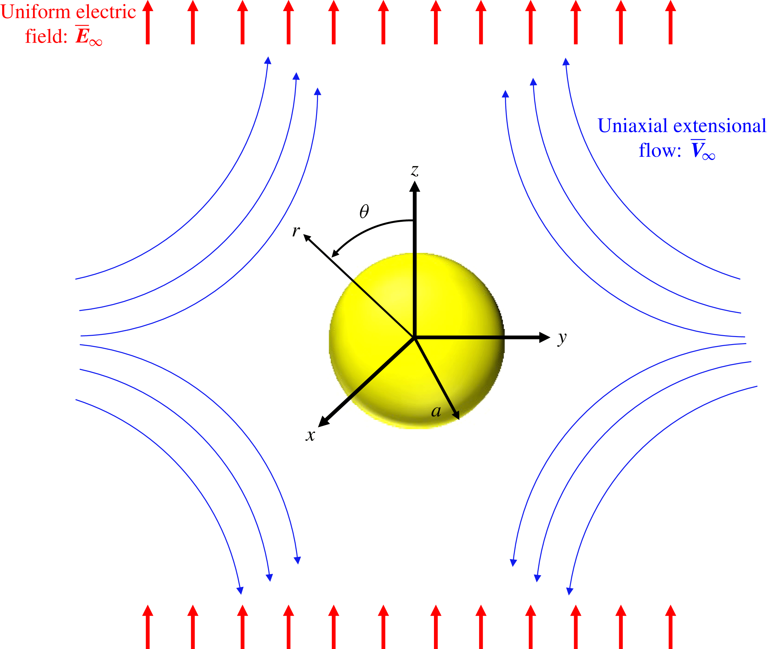
attached to the drop centroid (refer to figure 1).
Throughout our analysis we represent different quantities in dimensionless form unless otherwise mentioned. It is convenient to use the following non-dimensional scheme: length
 ${\sim}a$
, velocity
 ${\sim}Ga$
, electric field
 ${\sim}E_{\infty }$
, electric potential
 ${\sim}E_{\infty }a$
, hydrodynamic stress
 ${\sim}\unicode[STIX]{x1D707}_{e}G$
and electric stress
 ${\sim}\unicode[STIX]{x1D700}_{e}E_{\infty }^{2}$
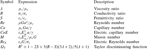
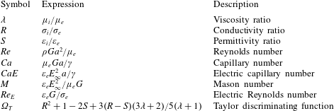
. The dimensionless problem is governed by the following material ratios and non-dimensional numbers (refer to table 1): viscosity ratio
 $\unicode[STIX]{x1D706}=\unicode[STIX]{x1D707}_{i}/\unicode[STIX]{x1D707}_{e}$
, conductivity ratio
 $R=\unicode[STIX]{x1D70E}_{i}/\unicode[STIX]{x1D70E}_{e}$
, permittivity ratio
 $S=\unicode[STIX]{x1D700}_{i}/\unicode[STIX]{x1D700}_{e}$
, Reynolds number
 $Re=\unicode[STIX]{x1D70C}Ga^{2}/\unicode[STIX]{x1D707}_{e}$
(signifies the strength of inertial stress relative to viscous stress), capillary number
 $Ca=\unicode[STIX]{x1D707}_{e}Ga/\unicode[STIX]{x1D6FE}$
(signifies the strength of viscous stress relative to the capillary stress), electric capillary number
 $Ca_{E}=\unicode[STIX]{x1D700}_{e}E_{\infty }^{2}a/\unicode[STIX]{x1D6FE}$
(signifies the strength of electric stress relative to capillary stress), electric Reynolds number
 $Re_{E}=\unicode[STIX]{x1D700}_{e}G/\unicode[STIX]{x1D70E}_{e}$
(signifies the strength of charge convection relative to the ohmic conduction) and Mason number
 $M=\unicode[STIX]{x1D700}_{e}E_{\infty }^{2}/\unicode[STIX]{x1D707}_{e}G$
(signifies the strength of electric stress relative to the viscous stress). Henceforth, subscripts ‘
 $i$
’ and ‘
 $e$
’ are used to represent different quantities inside and outside the drop, while subscripts ‘
 $r$
’ and ‘
 $\unicode[STIX]{x1D703}$
’ are used to represent corresponding r- and
 $\unicode[STIX]{x1D703}$
-components of a vector.
Schematic representation of a drop of radius
 $a$
which is encountering a uniform electric field
 $\bar{\boldsymbol{E}}_{\infty }$
and uniaxial extensional flow
 $\bar{\boldsymbol{V}}_{\infty }$
.

Important dimensionless numbers in the present analysis.
2.1 Governing equations and boundary conditions
Under the paradigm of the leaky dielectric model, the bulk fluid is charge free (Saville Reference Saville1997) and the electrostatic problem is governed by the Laplace equation for the electric potential both inside and outside the drop in the following form
 $$\begin{eqnarray}\unicode[STIX]{x1D6FB}^{2}\unicode[STIX]{x1D711}_{i}=0,\quad \unicode[STIX]{x1D6FB}^{2}\unicode[STIX]{x1D711}_{e}=0,\end{eqnarray}$$
where
 $\unicode[STIX]{x1D711}_{i}$
and
 $\unicode[STIX]{x1D711}_{i}$
represent the electric potential inside and outside the drop, respectively. The electric potential outside the drop (
 $\unicode[STIX]{x1D711}_{e}$
) is bounded and satisfies the following far-field condition
 $$\begin{eqnarray}\unicode[STIX]{x1D711}_{e}=-\boldsymbol{E}_{\infty }\boldsymbol{\cdot }\boldsymbol{x}=-r\cos \unicode[STIX]{x1D703}\quad \text{as}~r\rightarrow \infty .\end{eqnarray}$$
The electric potential inside the drop (
 $\unicode[STIX]{x1D711}_{i}$
) is bounded at the drop centre (
 $r=0$
). At the drop interface, the electric potential is continuous
 $$\begin{eqnarray}\unicode[STIX]{x1D711}_{i}=\unicode[STIX]{x1D711}_{e}\quad \text{at }r=r_{s}(\unicode[STIX]{x1D703}).\end{eqnarray}$$
Additionally, the electric potentials should satisfy the balance between ohmic conduction and charge convection at the drop interface (Mandal, Bandopadhyay & Chakraborty Reference Mandal, Bandopadhyay and Chakraborty2016b )
 $$\begin{eqnarray}\boldsymbol{n}\boldsymbol{\cdot }(R\unicode[STIX]{x1D735}\unicode[STIX]{x1D711}_{i}-\unicode[STIX]{x1D735}\unicode[STIX]{x1D711}_{e})=-Re_{E}\unicode[STIX]{x1D735}_{s}\boldsymbol{\cdot }(q_{s}\boldsymbol{V}_{s})\quad \text{at }r=r_{s}(\unicode[STIX]{x1D703}),\end{eqnarray}$$
where
 $q_{s}=\boldsymbol{n}\boldsymbol{\cdot }(S\unicode[STIX]{x1D735}\unicode[STIX]{x1D711}_{i}-\unicode[STIX]{x1D735}\unicode[STIX]{x1D711}_{e})|_{r=r_{s}}$
represents the surface charge distribution and
 $\boldsymbol{V}_{s}$
is the surface velocity. In (2.5),
 $\boldsymbol{n}=\unicode[STIX]{x1D735}(r-r_{s})/|\unicode[STIX]{x1D735}(r-r_{s})|$
represents the outward unit normal to the drop interface and
 $\unicode[STIX]{x1D735}_{s}=\unicode[STIX]{x1D735}-\boldsymbol{n}(\boldsymbol{n}\boldsymbol{\cdot }\unicode[STIX]{x1D735})$
represents the surface divergence operator. Note that if we substitute
 $R=S$
in the governing equations and the boundary conditions of the leaky dielectric system then the system is equivalent to a perfectly dielectric one (refer to appendix A for a detailed justification).
In the creeping flow limit (i.e.
 $Re=0$
), the flow problem is governed by the Stokes equation and the condition of incompressibility in the following form
 $$\begin{eqnarray}\left.\begin{array}{@{}c@{}}\unicode[STIX]{x1D735}p_{i}=\unicode[STIX]{x1D706}\unicode[STIX]{x1D6FB}^{2}\boldsymbol{u}_{i},\quad \unicode[STIX]{x1D735}\boldsymbol{\cdot }\boldsymbol{u}_{i}=0,\\ \unicode[STIX]{x1D735}p_{e}=\unicode[STIX]{x1D6FB}^{2}\boldsymbol{u}_{e},\quad \unicode[STIX]{x1D735}\boldsymbol{\cdot }\boldsymbol{u}_{e}=0,\end{array}\right\}\end{eqnarray}$$
where
 $p$
represents the pressure field and
 $\boldsymbol{u}=(u_{r},u_{\unicode[STIX]{x1D703}})$
represents the velocity field. Exploiting the symmetry of electric and flow problems about the z-axis, it is convenient to use the streamfunction
 $\unicode[STIX]{x1D6F9}$
which will simplify the mathematical calculations (Mandal, Bandopadhyay & Chakraborty Reference Mandal, Bandopadhyay and Chakraborty2017a
). The velocity components are related to the streamfunction as (Leal Reference Leal2007):
 $u_{r}=-(1/r^{2})\unicode[STIX]{x2202}\unicode[STIX]{x1D6F9}/\unicode[STIX]{x2202}\unicode[STIX]{x1D702}$
and
 $u_{\unicode[STIX]{x1D703}}=-(1/r\sqrt{1-\unicode[STIX]{x1D702}^{2}})\unicode[STIX]{x2202}\unicode[STIX]{x1D6F9}/\unicode[STIX]{x2202}r$
, where
 $\unicode[STIX]{x1D702}=\cos \unicode[STIX]{x1D703}$
is the transformed polar coordinate. The Stokes equations can be expressed in terms of the streamfunction (which automatically satisfies the incompressibility condition) in the following form
 $$\begin{eqnarray}{\mathcal{L}}^{2}({\mathcal{L}}^{2}\unicode[STIX]{x1D6F9}_{i})=0,\quad {\mathcal{L}}^{2}({\mathcal{L}}^{2}\unicode[STIX]{x1D6F9}_{e})=0,\end{eqnarray}$$
where
 ${\mathcal{L}}^{2}$
is a second-order linear operator of the form
 ${\mathcal{L}}^{2}=\unicode[STIX]{x2202}^{2}/\unicode[STIX]{x2202}r^{2}+\{(1-\unicode[STIX]{x1D702}^{2})/r^{2}\}\unicode[STIX]{x2202}^{2}/\unicode[STIX]{x2202}\unicode[STIX]{x1D702}^{2}$
. The velocity field outside the drop (
 $\boldsymbol{u}_{\boldsymbol{e}}$
) is bounded and satisfies the far-field condition
 $$\begin{eqnarray}\boldsymbol{u}_{e}=\unicode[STIX]{x1D71E}\boldsymbol{\cdot }\boldsymbol{x}\quad \text{as }r\rightarrow \infty .\end{eqnarray}$$
The velocity field inside the drop (
 $\boldsymbol{u}_{i}$
) is bounded at the drop centre (
 $r=0$
). At the drop interface, the velocity field is continuous and the normal component of the velocity field vanishes
 $$\begin{eqnarray}\left.\begin{array}{@{}c@{}}\boldsymbol{u}_{i}=\boldsymbol{u}_{e}\quad \text{at }r=r_{s}(\unicode[STIX]{x1D703}),\\ \boldsymbol{u}_{i}\boldsymbol{\cdot }\boldsymbol{n}=\boldsymbol{u}_{e}\boldsymbol{\cdot }\boldsymbol{n}=0\quad \text{at }r=r_{s}(\unicode[STIX]{x1D703}).\end{array}\right\}\end{eqnarray}$$
Additionally, the velocity and pressure fields should satisfy the balance of hydrodynamic, electric and capillary stresses at the drop interface
 $$\begin{eqnarray}(\unicode[STIX]{x1D749}_{e}^{H}+M\unicode[STIX]{x1D749}_{e}^{E})\boldsymbol{\cdot }\boldsymbol{n}-(\unicode[STIX]{x1D749}_{i}^{H}+M\unicode[STIX]{x1D749}_{i}^{E})\boldsymbol{\cdot }\boldsymbol{n}=\frac{1}{Ca}(\unicode[STIX]{x1D735}\boldsymbol{\cdot }\boldsymbol{n})\boldsymbol{n}\quad \text{at }r=r_{s}(\unicode[STIX]{x1D703}),\end{eqnarray}$$
where
 $\unicode[STIX]{x1D749}^{H}$
and
 $\unicode[STIX]{x1D749}^{E}$
are the hydrodynamic and electric stress tensors (Mandal, Chakrabarti & Chakraborty Reference Mandal, Chakrabarti and Chakraborty2017b
).
2.2 Expansion in perturbation of
 $Re_{E}$
and
$Ca$


A closer look into the electrostatic and flow problems reveals that both the electrostatic and flow problems are coupled and nonlinear in nature even though the governing equations are linear. The coupling between the electrostatic and flow problems stems from the nonlinear surface charge convection term (right-hand side of (2.5)). Another source of nonlinearity is present in all the interfacial boundary conditions due to the unknown shape of the drop (i.e. unknown
 $f$
(
 $\unicode[STIX]{x1D703}$
)). Thus the EHD of the drop in the combined presence of a uniform electric field and uniaxial extensional flow is not a mere linear superposition of the EHD of a drop in a uniform electric field and the hydrodynamics of drop in uniaxial extensional flow. Due to the two-way coupled and nonlinear nature of the problem, an analytical solution cannot, in general, be obtained for arbitrary values of
 $Re_{E}$
, Ca and
 $M$
. To proceed with an analytical treatment, in the present study we focus on the particular case in which
 $1\gg Re_{E}$
,
 $Ca\gg Re_{E}^{2}$
,
 $Re_{E}Ca$
,
 $Ca^{2}$
and
 $M\sim 1$
(Bandopadhyay et al.
Reference Bandopadhyay, Mandal, Kishore and Chakraborty2016). Physically it describes a system where the deformation of the drop is not far from a spherical shape and where the effect of the convection of the surface charges is weak as compared to the ohmic conduction.
 $M\sim 1$
represents the physical situation where the viscous stress and the electrical stress are of a comparable order of magnitude. These considerations allow us to represent any field variable
 $\unicode[STIX]{x1D712}$
in terms of a double asymptotic expansion using
 $Re_{E}$
and Ca as perturbation parameters in the following form:
 $$\begin{eqnarray}\unicode[STIX]{x1D712}=\unicode[STIX]{x1D712}^{(0)}+Re_{E}\unicode[STIX]{x1D712}^{(Re_{E})}+Ca\unicode[STIX]{x1D712}^{(Ca)}+\cdots \,,\end{eqnarray}$$
where
 $\unicode[STIX]{x1D712}^{(0)}$
is the leading-order contribution,
 $\unicode[STIX]{x1D712}^{(Re_{E})}$
is the
 $O(Re_{E})$
contribution and
 $\unicode[STIX]{x1D712}^{(Ca)}$
is the
 $O(Ca)$
contribution. Substituting the expansion given in (2.11) for all dependent variables into (2.2)–(2.10), one can easily obtain governing equations and respective boundary conditions at different orders of perturbation (Mandal, Bandopadhyay & Chakraborty Reference Mandal, Bandopadhyay and Chakraborty2016a
).
The unknown shape of the drop
 $r_{s}$
is also expanded as (Bandopadhyay et al.
Reference Bandopadhyay, Mandal, Kishore and Chakraborty2016)
 $$\begin{eqnarray}r_{s}=1+f(\unicode[STIX]{x1D703})=1+Caf^{(Ca)}+CaRe_{E}f^{(CaRe_{E})}+Ca^{2}f^{(Ca^{2})}+\cdots \,,\end{eqnarray}$$
where
 $f^{(Ca)}$
,
 $f^{(CaRe_{E})}$
and
 $f^{(Ca^{2})}$
are the corrections in drop shape due to leading-order,
 $O(Re_{E})$
and
 $O(Ca)$
electric and viscous stresses which are to be determined later by invoking normal stress balance.
3 Asymptotic solution for small charge convection and small shape deformation
Following reported studies (Xu & Homsy Reference Xu and Homsy2006; Mandal et al. Reference Mandal, Bandopadhyay and Chakraborty2016a ), we have obtained the analytical solution for the drop shape and emulsion rheology. The details of the solution are given in the supplementary document available at https://doi.org/10.1017/jfm.2017.897. Below we present important analytical expressions which are obtained from the analytical solution.
3.1 Drop shape
The
 $O(Ca)$
correction in drop shape is obtained as
 $$\begin{eqnarray}f^{(Ca)}=L_{2}^{(Ca)}P_{2}(\unicode[STIX]{x1D702}),\end{eqnarray}$$
where
 $P_{n}(\unicode[STIX]{x1D702})$
represents the
 $n$
th degree Legendre polynomial. The coefficient
 $L_{2}^{(Ca)}$
is obtained in the following form
 $$\begin{eqnarray}L_{2}^{(Ca)}=\frac{1}{8}\left(\frac{19\unicode[STIX]{x1D706}+16}{\unicode[STIX]{x1D706}+1}\right)+\frac{3}{4}\frac{M\unicode[STIX]{x1D6FA}_{T}}{(R+2)^{2}},\end{eqnarray}$$
where
 $\unicode[STIX]{x1D6FA}_{T}=R^{2}+1-2S+3(R-S)(3\unicode[STIX]{x1D706}+2)/5(\unicode[STIX]{x1D706}+1)$
is the Taylor discriminating function. The sole effect of the uniform electric field is to deform the drop into a prolate shape (represented by
 $\unicode[STIX]{x1D6FA}_{T}>0$
) or an oblate shape (represented by
 $\unicode[STIX]{x1D6FA}_{T}<0$
), while the sole effect of the extensional flow is always to deform the drop into a prolate shape. It is evident from (3.2) that the effect of the uniform electric field and uniaxial extensional flow on the drop shape combines linearly at this order.
The
 $O(CaRe_{E})$
correction in drop shape is obtained as
 $$\begin{eqnarray}f^{(CaRe_{E})}=L_{2}^{(CaRe_{E})}P_{2}(\unicode[STIX]{x1D702})+L_{4}^{(CaRe_{E})}P_{4}(\unicode[STIX]{x1D702}),\end{eqnarray}$$
where the coefficients
 $L_{2}^{(CaRe_{E})}$
and
 $L_{4}^{(CaRe_{E})}$
are obtained as
 $$\begin{eqnarray}L_{2}^{(CaRe_{E})}=M(R-S)\ell _{1},\quad L_{4}^{(CaRe_{E})}=M(R-S)\ell _{2},\end{eqnarray}$$
where
 $\ell _{1}$
and
 $\ell _{2}$
are known functions of
 $R$
,
 $S$
,
 $\unicode[STIX]{x1D706}$
and
 $M$
which we have given in appendix B.
The
 $O(Ca^{2})$
correction in drop shape is obtained as
 $$\begin{eqnarray}f^{(Ca^{2})}=L_{2}^{(Ca^{2})}P_{2}(\unicode[STIX]{x1D702})+L_{4}^{(Ca^{2})}P_{4}(\unicode[STIX]{x1D702}),\end{eqnarray}$$
where the coefficients
 $L_{2}^{(Ca^{2})}$
and
 $L_{4}^{(Ca^{2})}$
are obtained as
 $$\begin{eqnarray}L_{2}^{(Ca^{2})}=L_{2}^{(Ca)}(\ell _{3}+\ell _{4}L_{2}^{(Ca)}),\quad L_{4}^{(Ca^{2})}=L_{2}^{(Ca)}(\ell _{5}+\ell _{6}L_{2}^{(Ca)}),\end{eqnarray}$$
where
 $\ell _{3}{-}\ell _{6}$
are known functions of
 $R$
,
 $S$
,
 $\unicode[STIX]{x1D706}$
and
 $M$
which we have given in appendix B.
Now, substituting
 $f^{(Ca)}$
,
 $f^{(CaRe_{E})}$
and
 $f^{(Ca^{2})}$
in (2.12), we obtain the deformed drop shape as
 $$\begin{eqnarray}\displaystyle r_{s} & = & \displaystyle \left[1+CaL_{2}^{(Ca)}P_{2}(\unicode[STIX]{x1D702})+CaRe_{E}\left\{L_{2}^{(CaRe_{E})}P_{2}(\unicode[STIX]{x1D702})+L_{4}^{\left(CaRe_{E}\right)}P_{4}(\unicode[STIX]{x1D702})\right\}\right.\nonumber\\ \displaystyle & & \displaystyle +\,\left.Ca^{2}\left\{c_{v}+L_{2}^{(Ca^{2})}P_{2}\left(\unicode[STIX]{x1D702}\right)+L_{4}^{(Ca^{2})}P_{4}(\unicode[STIX]{x1D702})\right\}\right].\end{eqnarray}$$
The term
 $c_{v}=-(L_{2}^{(Ca)})^{2}/5$
is included at
 $O(Ca^{2})$
to conserve the drop volume. When the drop shape is nearly spherical, the degree of drop deformation is characterized by the deformation parameter of the form
 ${\mathcal{D}}=\left(L-B\right)/\left(L+B\right)$
, where
 $L=r_{s}\left(\unicode[STIX]{x1D703}=0\right)$
and
 $B=r_{s}\left(\unicode[STIX]{x1D703}=\unicode[STIX]{x03C0}/2\right)$
are the semi-major and semi-minor axes of the deformed ellipsoidal drop shape. The deformation parameter
 ${\mathcal{D}}>0$
represents the prolate shape of the drop, while
 ${\mathcal{D}}<0$
represents the oblate shape of the drop. We obtain the expression for the deformation parameter which includes the combined effect of the uniform electric field and uniaxial extensional flow as
 $$\begin{eqnarray}\displaystyle {\mathcal{D}} & = & \displaystyle \displaystyle \frac{3L_{2}^{(Ca)}Ca}{4}+\left\{\frac{3L_{2}^{(CaRe_{E})}}{4}+\frac{5L_{4}^{(CaRe_{E})}}{16}\right\}CaRe_{E}\nonumber\\ \displaystyle & & \displaystyle +\displaystyle \,\left\{\frac{3L_{2}^{\left(Ca^{2}\right)}}{4}+\frac{5L_{4}^{(Ca^{2})}}{16}-\frac{3\left(L_{2}^{(Ca)}\right)^{2}}{16}\right\}Ca^{2}.\end{eqnarray}$$
3.2 Emulsion extensional rheology
Presence of a uniform electric field affects both the flow around the drop and drop shape. The altered flow field and drop shape can affect the rheological properties of a dilute suspension of Newtonian drops in the presence of a background uniaxial extensional flow. Here, we focus on the emulsion stress for a dilute emulsion with
 $\unicode[STIX]{x1D708}\ll 1$
, where
 $\unicode[STIX]{x1D708}$
is the drop volume fraction. The effective suspension stress
 $\unicode[STIX]{x1D6F4}$
for a dilute suspension of drops in linear flow is given as (Barthès-Biesel Reference Barthès-Biesel2012)
 $\unicode[STIX]{x1D6F4}=-p\boldsymbol{I}+2\unicode[STIX]{x1D71E}+\unicode[STIX]{x1D72E}^{(d)}$
, where
 $\unicode[STIX]{x1D72E}^{(d)}$
is the stresslet tensor. The stresslet tensor
 $\unicode[STIX]{x1D72E}^{(d)}$
can be represented in the following form (Barthès-Biesel Reference Barthès-Biesel2012)
 $$\begin{eqnarray}\unicode[STIX]{x1D72E}^{(d)}=\frac{3\unicode[STIX]{x1D708}}{4\unicode[STIX]{x03C0}}\int _{S_{d}}\left[\frac{1}{2}\left\{\left(\unicode[STIX]{x1D749}_{e}^{H}\boldsymbol{\cdot }\boldsymbol{n}\right)\boldsymbol{r}+\left(\left(\unicode[STIX]{x1D749}_{e}^{H}\boldsymbol{\cdot }\boldsymbol{n}\right)\boldsymbol{r}\right)^{\text{T}}-\frac{2}{3}\boldsymbol{I}\left(\unicode[STIX]{x1D749}_{e}^{H}\boldsymbol{\cdot }\boldsymbol{n}\right)\boldsymbol{\cdot }\boldsymbol{r}\right\}-\left(\boldsymbol{u}_{e}\boldsymbol{n}+\left(\boldsymbol{u}_{e}\boldsymbol{n}\right)^{\text{T}}\right)\right]\text{d}S_{d},\end{eqnarray}$$
where
 $S_{d}$
is the deformed drop surface. The stresslet tensor is generated due to the presence of suspended drops. Both charge convection and shape deformation affect the stresslet tensor. To quantify these effects, it is convenient for extensional flow to define a dimensional extensional viscosity
 $\unicode[STIX]{x1D707}_{ext}$
of the dilute suspension as
 $\unicode[STIX]{x1D707}_{ext}=(\bar{\unicode[STIX]{x1D6F4}}_{zz}-\bar{\unicode[STIX]{x1D6F4}}_{xx})/G=(\bar{\unicode[STIX]{x1D6F4}}_{zz}-\bar{\unicode[STIX]{x1D6F4}}_{yy})/G$
, where the dimensional stress component
 $\bar{\unicode[STIX]{x1D6F4}}_{ij}$
can be expressed as
 $\bar{\unicode[STIX]{x1D6F4}}_{ij}=\unicode[STIX]{x1D707}_{e}G\unicode[STIX]{x1D6F4}_{ij}$
. Now, substituting different terms we obtain the extensional viscosity ratio (also termed Trouton’s ratio which is defined as the ratio between extensional viscosity and shear viscosity) as
 $\unicode[STIX]{x1D702}_{ext}=\unicode[STIX]{x1D707}_{ext}/\unicode[STIX]{x1D707}_{e}=\unicode[STIX]{x1D702}_{ext}^{(0)}+Re_{E}\unicode[STIX]{x1D702}_{ext}^{\left(Re_{E}\right)}+Ca\unicode[STIX]{x1D702}_{ext}^{(Ca)}$
, where
 $\unicode[STIX]{x1D702}_{ext}^{\left(0\right)}$
represents the extensional viscosity ratio when the charge convection and shape deformation effects are absent,
 $\unicode[STIX]{x1D702}_{ext}^{\left(Re_{E}\right)}$
and
 $\unicode[STIX]{x1D702}_{ext}^{(Ca)}$
represent the explicit effect of charge convection and shape deformation on the extensional viscosity ratio. Expressions for
 $\unicode[STIX]{x1D702}_{ext}^{(0)}$
,
 $\unicode[STIX]{x1D702}_{ext}^{\left(Re_{E}\right)}$
and
 $\unicode[STIX]{x1D702}_{ext}^{(Ca)}$
are obtained as
 $$\begin{eqnarray}\displaystyle \left.\begin{array}{@{}c@{}}\displaystyle \unicode[STIX]{x1D702}_{ext}^{(0)}=3+\unicode[STIX]{x1D708}\left[\frac{3}{2}\frac{\left(5\unicode[STIX]{x1D706}+2\right)}{\left(\unicode[STIX]{x1D706}+1\right)}+\frac{27}{5}\frac{M\left(S-R\right)}{\left(R+2\right)^{2}\left(\unicode[STIX]{x1D706}+1\right)}\right],\\[14.0pt] \displaystyle \unicode[STIX]{x1D702}_{ext}^{\left(Re_{E}\right)}=\unicode[STIX]{x1D708}\left[\frac{81M\left(R-S\right)\left\{5\left(R+2\right)^{2}+6M(R-S)\right\}\left(69R^{2}+130R-54SR-80S+40\right)}{875\left(\unicode[STIX]{x1D706}+1\right)^{2}\left(3R+4\right)\left(R+2\right)^{5}}\right],\\[21.0pt] \displaystyle \unicode[STIX]{x1D702}_{ext}^{(Ca)}=\unicode[STIX]{x1D708}\left[L_{2}^{(Ca)}\left(\frac{9}{70}\frac{41\unicode[STIX]{x1D706}+4+25\unicode[STIX]{x1D706}^{2}}{\left(1+\unicode[STIX]{x1D706}\right)^{2}}-\frac{162}{175}\frac{M(R-S)\left(13\unicode[STIX]{x1D706}R+15R-12-16\unicode[STIX]{x1D706}\right)}{\left(1+\unicode[STIX]{x1D706}\right)^{2}\left(R+2\right)^{3}}\right)\right].\end{array}\right\} & & \displaystyle \nonumber\\ \displaystyle & & \displaystyle\end{eqnarray}$$
4 Numerical simulation
To study the drop deformation beyond the small deformation limit, we use the open source code Gerris (http://gfs.sf.net) developed by Popinet (Reference Popinet2003, Reference Popinet2009) and others (López-Herrera, Popinet & Herrada Reference López-Herrera, Popinet and Herrada2011). We use the Electrohydro module of Gerris which solves the coupled nonlinear EHD system by using the finite-volume method (López-Herrera et al.
Reference López-Herrera, Popinet and Herrada2011). A volume-of-fluid method (VOF) is used to capture the fluid–fluid interface by solving an advection equation for the volume fraction (
 $c$
) as
 $$\begin{eqnarray}\frac{\unicode[STIX]{x2202}c}{\unicode[STIX]{x2202}t}+\unicode[STIX]{x1D735}\boldsymbol{\cdot }\left(c\boldsymbol{u}\right)=0.\end{eqnarray}$$
The electric potential (
 $\unicode[STIX]{x1D711}$
) and charge density (
 $q_{v}$
) are obtained by solving a Poisson equation for electric potential and a charge transport equation in the following form (López-Herrera et al.
Reference López-Herrera, Popinet and Herrada2011)
 $$\begin{eqnarray}\unicode[STIX]{x1D735}\boldsymbol{\cdot }\left(\unicode[STIX]{x1D700}\unicode[STIX]{x1D735}\unicode[STIX]{x1D711}\right)=-q_{v},\quad Re_{E}\left[\frac{\unicode[STIX]{x2202}q_{v}}{\unicode[STIX]{x2202}t}+\unicode[STIX]{x1D735}\boldsymbol{\cdot }\left(q_{v}\boldsymbol{u}\right)\right]=\unicode[STIX]{x1D735}\boldsymbol{\cdot }\left(\unicode[STIX]{x1D70E}\unicode[STIX]{x1D735}\unicode[STIX]{x1D711}\right),\end{eqnarray}$$
where the variation of permittivity and conductivity are taken as
 $\unicode[STIX]{x1D700}=cS+(1-c)$
and
 $\unicode[STIX]{x1D70E}=cR+(1-c)$
(López-Herrera et al.
Reference López-Herrera, Popinet and Herrada2011). Important to note is that the numerical simulations deal with the volumetric charge density
 $q_{v}$
instead of surface charge density
 $q_{s}$
. However, for relatively small values of
 $Re_{E}$
, the charges will be accumulated at the drop interface quickly and the volumetric charge transport equivalently represents the surface charge transport. The flow field is obtained by solving the continuity equation and the Navier–Stokes equation in the following form (López-Herrera et al.
Reference López-Herrera, Popinet and Herrada2011)
 $$\begin{eqnarray}\left.\begin{array}{@{}c@{}}\unicode[STIX]{x1D735}\boldsymbol{\cdot }\boldsymbol{u}=0,\\ \displaystyle Re\left(\frac{\unicode[STIX]{x2202}\boldsymbol{u}}{\unicode[STIX]{x2202}t}+\boldsymbol{u}\boldsymbol{\cdot }\unicode[STIX]{x1D735}\boldsymbol{u}\right)=-\unicode[STIX]{x1D735}p+\unicode[STIX]{x1D735}\boldsymbol{\cdot }\left[\unicode[STIX]{x1D707}\left\{\unicode[STIX]{x1D735}\boldsymbol{u}+\left(\unicode[STIX]{x1D735}\boldsymbol{u}\right)^{\text{T}}\right\}\right]+M\boldsymbol{F}^{e}+\frac{1}{Ca}\boldsymbol{F}_{s},\end{array}\right\}\end{eqnarray}$$
where
 $\boldsymbol{F}_{s}$
is the surface tension force and
 $\boldsymbol{F}_{e}$
is the electric force. The variation of viscosity is taken as
 $\unicode[STIX]{x1D707}=c\unicode[STIX]{x1D706}+(1-c)$
.
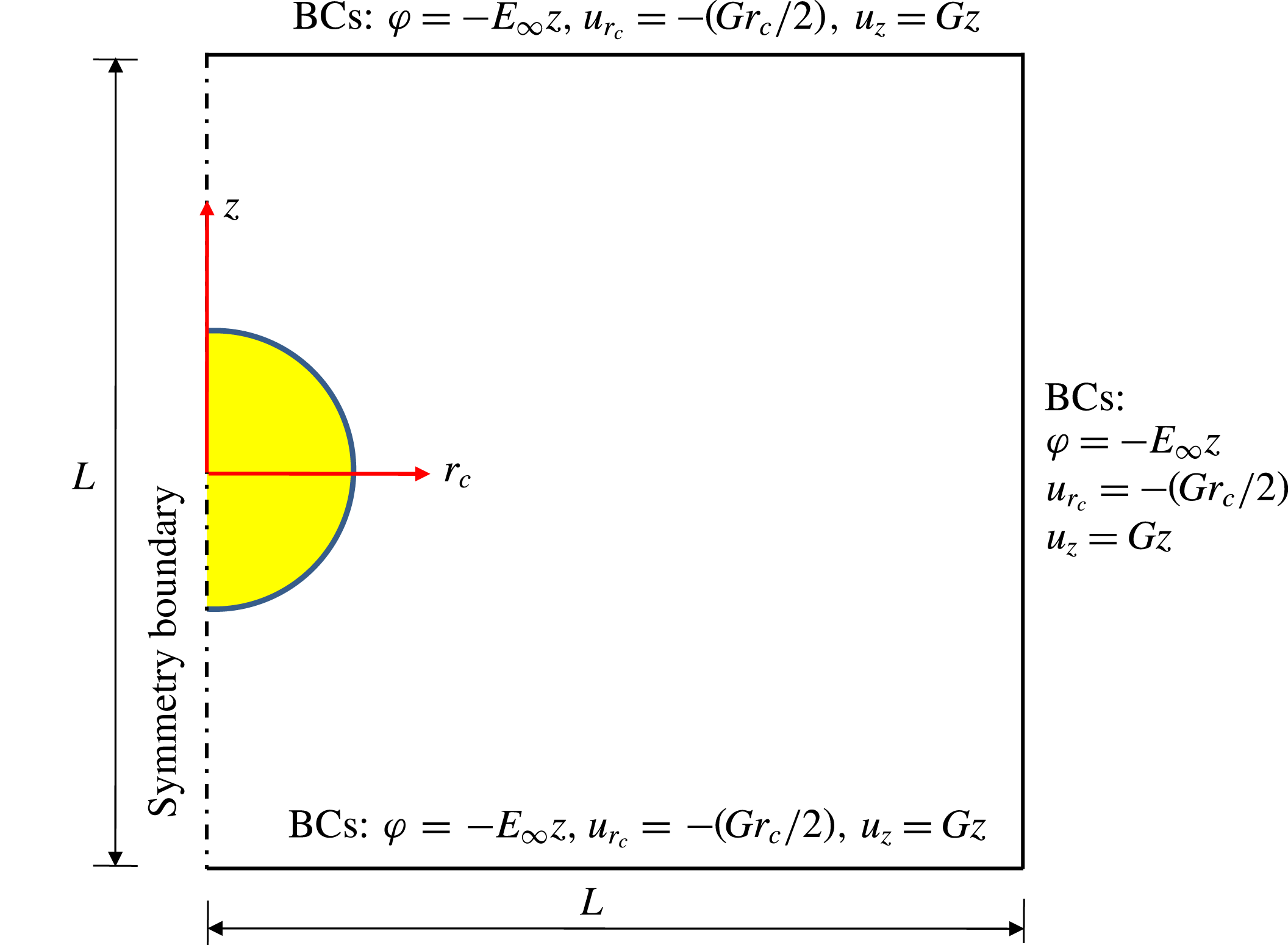
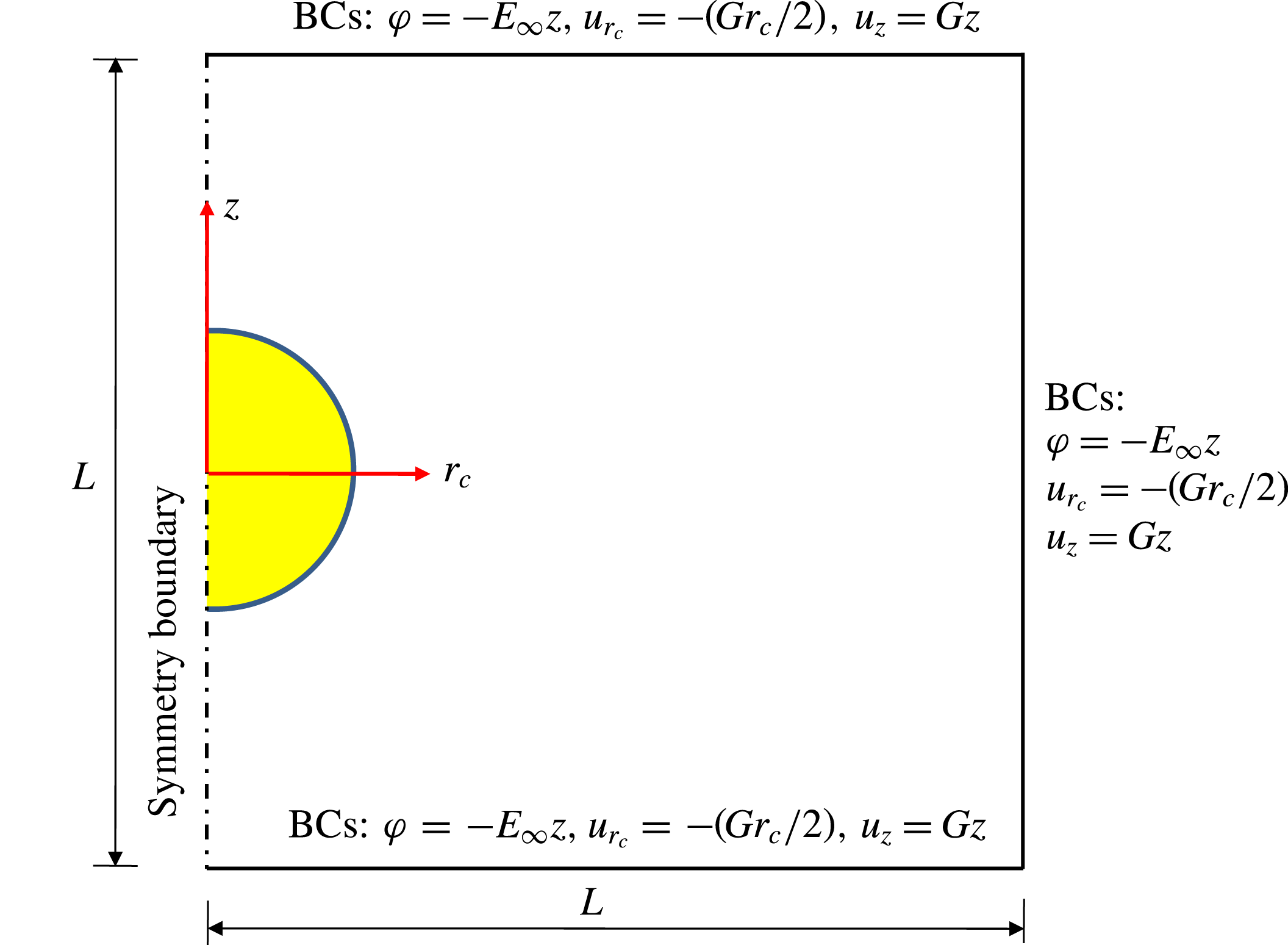
The simulations are performed on two-dimensional axisymmetric domain (
 $r_{c}$
,
 $z$
) of size
 $L\times L$
as depicted in figure 2. The boundary conditions are shown in figure 2. To minimize the effect of domain confinement, we use
 $L=10$
which is discretized using quadtree mesh (Popinet Reference Popinet2003). To reduce the computational cost and to capture the charge transport near the fluid–fluid interface, we use the gradient-based adaptive mesh refinement (Popinet Reference Popinet2003) feature of Gerris which employs a finer mesh near the fluid–fluid interface and a relatively coarse mesh in the bulk. After performing a grid independent study, we have taken a mesh size of
 $\unicode[STIX]{x0394}r_{c}=\unicode[STIX]{x0394}z=L\times 2^{-10}$
(where 10 represents the maximum refinement level) near the interface and a mesh size of
 $\unicode[STIX]{x0394}r_{c}=\unicode[STIX]{x0394}z=L\times 2^{-6}$
(where 6 represents the minimum refinement level) in the bulk. To simulate the physical situation of negligible fluid inertia, we have considered
 $Re=0.01$
for all numerical simulations.
Schematic representation of the simulation domain. An axisymmetric domain of rectangular size
 $L\times L$
in cylindrical coordinates
 $(r_{c},z)$
is considered.
5 Results and discussion
5.1 Validation
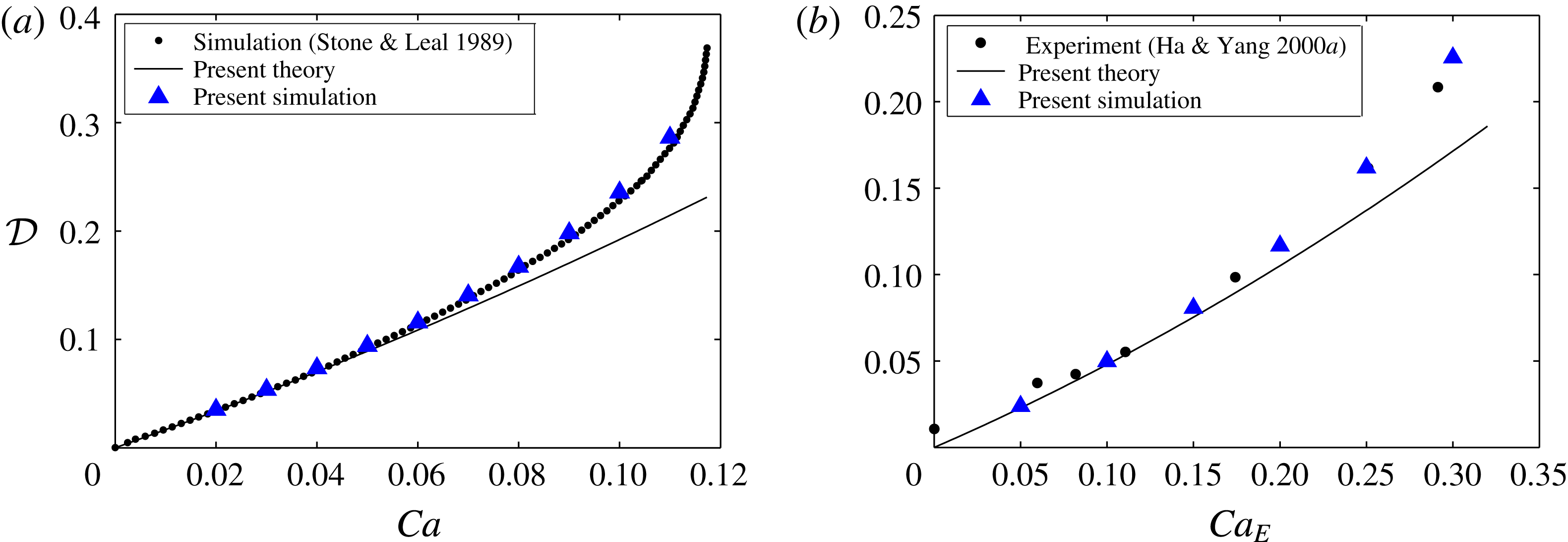
Before investigating the combined influence of uniaxial extensional flow and uniform electric field, we compare our theoretical and numerical results with the existing results for the following two limiting cases: (i) drop deformation in a uniaxial extensional flow, and (ii) drop deformation in a uniform electric field. When the electric field is absent, the present analytical result for drop deformation recovers the analytical result of Barthés-Biesel & Acrivos (Reference Barthés-Biesel and Acrivos1973).
Figure 3(a) depicts the variation of drop deformation with capillary number in uniaxial extensional flow. It is evident that the present analytical result compares very well with the numerical result of Stone & Leal (Reference Stone and Leal1989) for small values of Ca. With increase in Ca, the analytical result underpredicts the deformation. However, our numerical solution compares very well even in the large deformation regime. When the extensional flow is absent, the present analytical result for drop deformation recovers the analytical result of Ajayi (Reference Ajayi1978) and Feng (Reference Feng1999). Figure 3(b) depicts the variation of drop deformation with electric capillary number (
 $Ca_{E}=\unicode[STIX]{x1D700}_{e}E_{\infty }^{2}a/\unicode[STIX]{x1D6FE}$
) in a uniform electric field. Note that
 $Ca_{E}$
represents the strength of electric stress (which tries to deform the drop) relative to the capillary stress (which resists the drop deformation). Similar to the drop deformation in uniaxial extensional flow, the present analytical result compares very well with the experimental result of Ha & Yang (Reference Ha and Yang2000a
) for small values of
 $Ca_{E}$
. However, the agreement between our numerical result and the experiment of Ha & Yang (Reference Ha and Yang2000a
) is over the whole
 $Ca_{E}$
regime under consideration.
(a) Variation of droplet deformation with capillary number in uniaxial extensional flow for
 $\unicode[STIX]{x1D706}=1$
. (b) Variation of droplet deformation with electric capillary number in uniform electric field for
 $R=10$
,
 $S=1.37$
,
 $\unicode[STIX]{x1D706}=0.874$
and
 $Re_{E}=0.01$
. We consider
 $Re=0.01$
for all the simulations to simulate low Reynolds number flow.

5.2 Combined effect of uniform electric field and uniaxial extensional flow on the drop deformation
5.2.1 Asymptotic theory
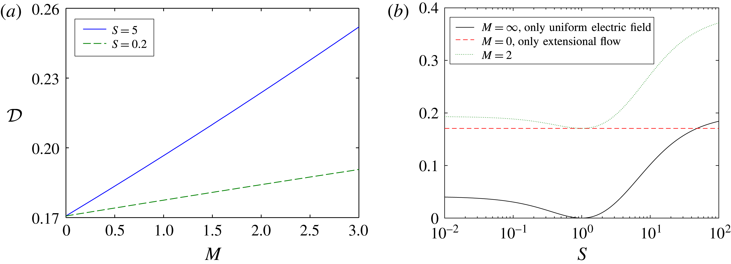
Figure 4(a) shows the variation of drop deformation with Mason number for a perfectly dielectric drop which is suspended in another perfectly dielectric medium (PD–PD system). Although the analytical solution is obtained for a leaky dielectric drop suspended in a leaky dielectric medium (LD–LD system), substitution of
 $R=S$
into (3.8) yields the drop deformation for the PD–PD system. Note that
 $M=0$
represents the absence of electric field (i.e. only extensional flow), while
 $M>0$
represents the combined presence of electric field and extensional flow. Figure 4(a) shows that drop deformation increases with increase in
 $M$
(which represents increasing strength of electric field as compared to strain rate) for both values of the permittivity ratio. This increase in drop deformation with increase in Mason number can be explained by the fact that the independent effect of extensional flow and uniform electric field is to deform the drop into a prolate shape. Thus, the combined effect leads to larger deformation.
(a) Variation of drop deformation with Mason number for
 $Ca=0.1$
and
 $\unicode[STIX]{x1D706}=0.1$
. (b) Variation of drop deformation with permittivity ratio for
 $Ca=0.1$
and
 $\unicode[STIX]{x1D706}=0.1$
.

(a) Schematic representation of streamline in and around the drop in extensional flow. Variation of the jump in electric traction on the drop surface for (b)
 $S=5$
and (c)
 $S=0.2$
.

To investigate the effect of permittivity ratio on the drop deformation, we plot the variation of drop deformation with the permittivity ratio for the PD–PD system in figure 4(b). We have also plotted the electric-field-induced drop deformation which is the
 $M=\infty$
limit (i.e. absence of imposed extensional flow). Figure 4(b) shows that drop always deforms to a prolate shape (irrespective of the value of
 $S$
) in the combined presence of an electric field and extensional flow. Figure 4(b) also shows that in the combined presence of a uniform electric field and extensional flow, the drop deformation is always larger as compared with either electric-field-induced or extensional-flow-induced drop deformation.
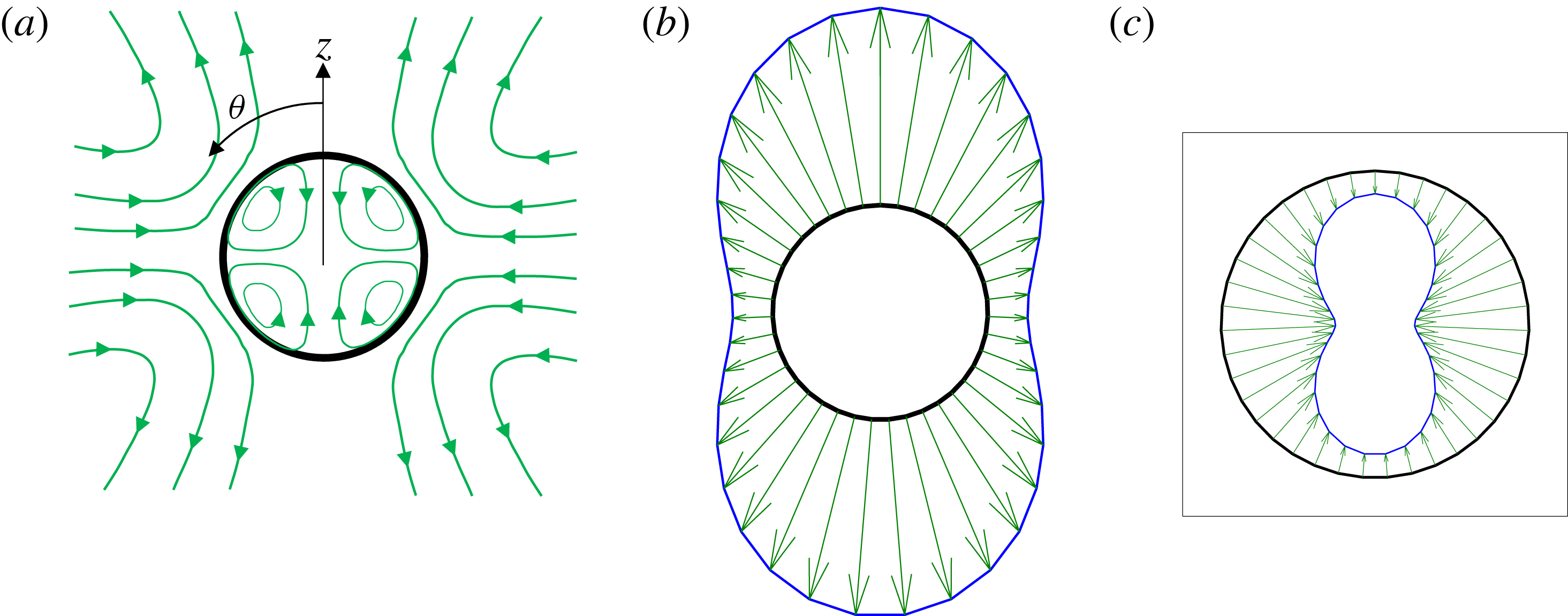
The physical reason for the prolate deformation of a PD drop and associated variation with permittivity ratio in the combined presence of electric field and extensional flow can be understood if we look into the independent effects of extensional flow and uniform electric field. The extensional-flow-induced drop deformation is due to the jump in the normal component of hydrodynamic traction. Figure 5(a) depicts a schematic drawing of the streamline pattern due to the imposed extensional flow. The flow at the drop surface is directed from the equator (
 $\unicode[STIX]{x1D703}=\unicode[STIX]{x03C0}/2$
) towards the poles (
 $\unicode[STIX]{x1D703}=0,\unicode[STIX]{x03C0}$
) and this kind of flow is always associated with a jump in hydrodynamic traction which stretches the drop along the extension axis (i.e. prolate shape). On the other hand, the electric-field-induced deformation is due to the jump in normal component of electric traction. The distribution of the jump in the normal component of electric traction at the drop surface is shown in figure 5(b) for
 $S=5$
and figure 5(c) for
 $S=0.2$
. The jump in normal electric traction for
 $S=5$
is radially outward and largest near the poles (
 $\unicode[STIX]{x1D703}=0,\unicode[STIX]{x03C0}$
), while the magnitude reduces near the equator (
 $\unicode[STIX]{x1D703}=\unicode[STIX]{x03C0}/2$
). Thus for
 $S=5$
the drop is stretched near the poles (the same is true for
 $S>1$
). On the other hand, the jump in electric traction for
 $S=0.2$
is radially inward and largest near the equator (
 $\unicode[STIX]{x1D703}=\unicode[STIX]{x03C0}/2$
), while the magnitude reduces near the poles (
 $\unicode[STIX]{x1D703}=0,\unicode[STIX]{x03C0}$
). Thus for
 $S=0.2$
the drop is compressed near the equator (the same is true for
 $S<1$
). In both cases the drop is deformed into a prolate shape. The permittivity ratio has a large impact on the electric-field-induced drop deformation (as depicted in figure 4
b) due to the dependence of electric traction on the permittivity ratio. Permittivity ratio significantly modulates the field lines near the drop surface. For example, when
 $S>1$
(or
 $S<1$
) the density of field lines inside the drop is smaller (or larger) than outside. For the particular case of
 $S=1$
, the field lines are not at all distorted by the drop and the jump in electric traction vanishes. Thus for
 $S=1$
the electric field has no effect on the drop deformation. So, the independent effect of the extensional flow and electric field is always to deform the drop into a prolate shape. For given values of Ca and
 $\unicode[STIX]{x1D706}$
, there is a critical permittivity ratio beyond which the electric-field-induced drop deformation is larger than the extensional-flow-induced drop deformation. This is due to the larger magnitude of the jump in the normal component of electric traction as compared with the jump in the normal component of hydrodynamic traction. In the combined presence of a uniform electric field and extensional flow, the drop deformation is always larger as compared with either electric-field-induced or extensional-flow-induced drop deformation. However, for
 $S=1$
the jump in electric traction vanishes and only the extensional flow deforms the drop. This explains the fact that the drop deformation with
 $M=2$
and
 $S=1$
is exactly equal to the drop deformation solely due to extensional flow as depicted in figure 4(b).
(a) Variation of drop deformation with Mason number for
 $Ca=Re_{E}=\unicode[STIX]{x1D706}=0.1$
. (b) Variation of drop deformation with conductivity ratio for
 $Ca=Re_{E}=\unicode[STIX]{x1D706}=0.1$
and
 $M=1$
.

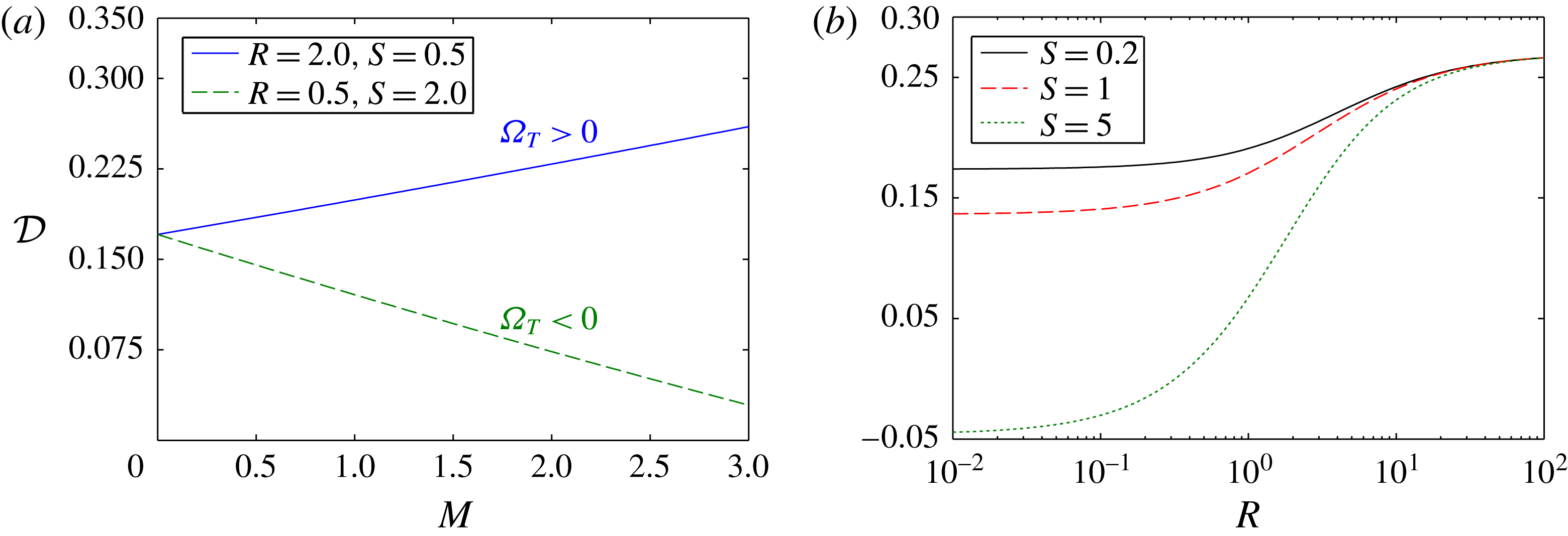
The deformation behaviour of LD–LD system is depicted in figure 6(a) where we have shown the variation of drop deformation with the Mason number. Figure 6(a) shows that the drop deformation increases with the Mason number for
 $(R,S)=(2.0,0.5)$
. This is due to the positive value of the Taylor discriminating function (
 $\unicode[STIX]{x1D6FA}_{T}>0$
), which means the electric field favours prolate deformation. Thus, similar to the PD–PD system, both the extensional flow and electric field deform the drop into a prolate shape for
 $\unicode[STIX]{x1D6FA}_{T}>0$
. However, in sharp contrast to the PD–PD system, the drop deformation decreases with the Mason number for
 $(R,S)=(0.5,2.0)$
. This is due to the negative value of the Taylor discriminating function (
 $\unicode[STIX]{x1D6FA}_{T}<0$
) which means the electric field favours oblate deformation. So, for
 $\unicode[STIX]{x1D6FA}_{T}<0$
the electric-field-induced and extensional-flow-induced drop deformations are opposite to each other. For smaller values of
 $M$
, extensional flow dominates over the electric field and the drop deforms to a prolate shape as depicted in figure 6(a). However, for relatively larger values of
 $M$
, the electric field dominates over the extensional flow and the drop may deform into an oblate shape. To investigate the effect of electrical parameters, we plot the variation of drop deformation with the conductivity ratio (
 $R$
) for different values of permittivity ratio (
 $S$
) in figure 6(b). The first important thing to note from figure 6(b) is that, depending on the values of
 $R$
and
 $S$
, the drop can deform into a prolate or oblate shape in the combined presence of an electric field and extensional flow. For
 $R\gg 1$
the drop deformation is independent of
 $S$
. This is due to the fact that in the limit
 $R\rightarrow \infty$
, the drop behaves as a perfectly conducting drop. For a perfectly conducting drop, the drop surface becomes an equipotential surface. The electric field inside the drop vanishes which means the electric permittivity of the drop fluid has no impact on the distribution of electric potential and electric traction. Electric permittivity has a noteworthy impact on the drop deformation when
 $R\ll 1$
as depicted in figure 6(b).
Variation of drop deformation with Mason number for (a)
 $(R,S)=(2.0,0.5)$
and (b)
 $(R,S)=(0.1,2.0)$
. Other parameters are taken as
 $\unicode[STIX]{x1D706}=0.1$
and
 $Ca=0.1$
.

To study the pivotal role of surface charge convection in the drop deformation, we show the drop deformation in the presence of surface charge convection (i.e.
 $Re_{E}>0$
) and compare it with the case of no surface charge convection (i.e.
 $Re_{E}=0$
). Previous studies on drop deformation in a uniform electric field established the fact that surface charge convection has a strong influence on the drop deformation (Lanauze et al.
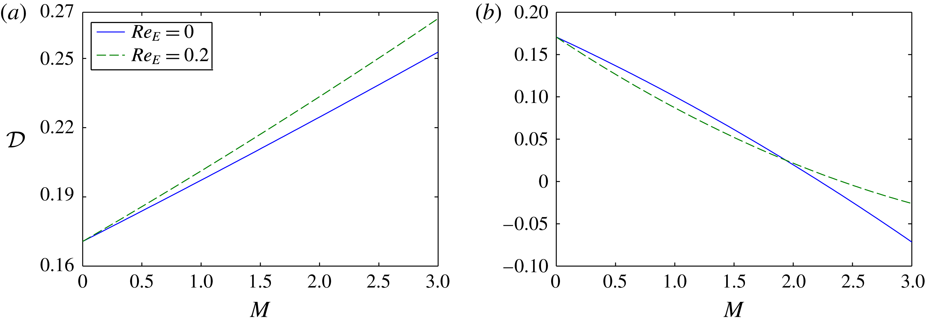
Reference Lanauze, Walker and Khair2015; Das & Saintillan Reference Das and Saintillan2017). In the combined presence of a uniform electric field and extensional flow, we first plot the variation of drop deformation with Mason number considering
 $(R,S)=(2,0.5)$
in figure 7(a). Figure 7(a) shows that the charge convection increases the drop deformation. Surface charge convection leads to a greater increase in drop deformation for larger values of the Mason number. Figure 7(b) shows that the charge convection can decrease or increase the drop deformation depending on the value of Mason number for
 $(R,S)=(0.1,2.0)$
. A closer look into figure 7(b) shows that when the drop deforms into prolate shape, the charge convection can either decrease (for
 $M=1$
) or increase (for
 $M=2$
) the drop deformation. But when the drop deforms into an oblate shape, the charge convection always decreases the drop deformation (e.g.
 $M=3$
).
Schematic representation of two different types of EHD flow in and around drop in the presence of a uniform electric field for (a)
 $R>S$
and (b)
 $R<S$
.

Previous studies on the drop deformation in a uniform electric field have established the fact that charge convection enhances prolate deformation, while it acts to reduce the oblate deformation (Feng Reference Feng1999). However, in the combined presence of a uniform electric field and uniaxial extensional flow, we obtain either an increase or decrease in drop deformation due to charge convection when the drop is deformed into a prolate shape, while an oblate drop is found to deform less in the presence of charge convection. To investigate the physical reason for the charge-convection-induced increase/decrease in drop deformation, we consider two different cases: (i)
 $R>S$
(e.g.
 $R=2$
and
 $S=0.5$
), (ii)
 $R<S$
(e.g.
 $R=0.1$
and
 $S=2$
). To understand the charge-convection-induced drop deformation, we look into the effect of fluid flow on the distribution of surface charges. In the absence of convection, the surface charge distribution is governed by the ohmic conduction (Salipante & Vlahovska Reference Salipante and Vlahovska2010). The distribution of charges at the drop surface is governed by the ratio
 $R/S=t_{e}/t_{i}$
, where
 $t_{e}=(\unicode[STIX]{x1D700}_{e}/\unicode[STIX]{x1D70E}_{e})$
and
 $t_{i}=(\unicode[STIX]{x1D700}_{i}/\unicode[STIX]{x1D70E}_{i})$
are the charge relaxation time scales of suspending phase and drop phase, respectively. Charge relaxation time scale physically signifies the time required for charges to reach a steady configuration due to ohmic conduction (Melcher & Taylor Reference Melcher and Taylor1969). For
 $R>S$
or equivalently
 $t_{i}<t_{e}$
the ohmic conduction in the drop phase is much faster (due to small time scale) than the ohmic conduction in the suspending phase. Consequence of this is the charging of the drop surface by the bulk charges coming from the drop phase. In the presence of a uniform electric field acting along the positive
 $z$
direction, the fast conduction in the drop phase leads to accumulation of positive charges at the upper hemispherical surface (
 $0\leqslant \unicode[STIX]{x1D703}<\unicode[STIX]{x03C0}/2$
), while negative charges accumulate at the lower hemispherical surface (
 $\unicode[STIX]{x03C0}/2<\unicode[STIX]{x1D703}\leqslant \unicode[STIX]{x03C0}$
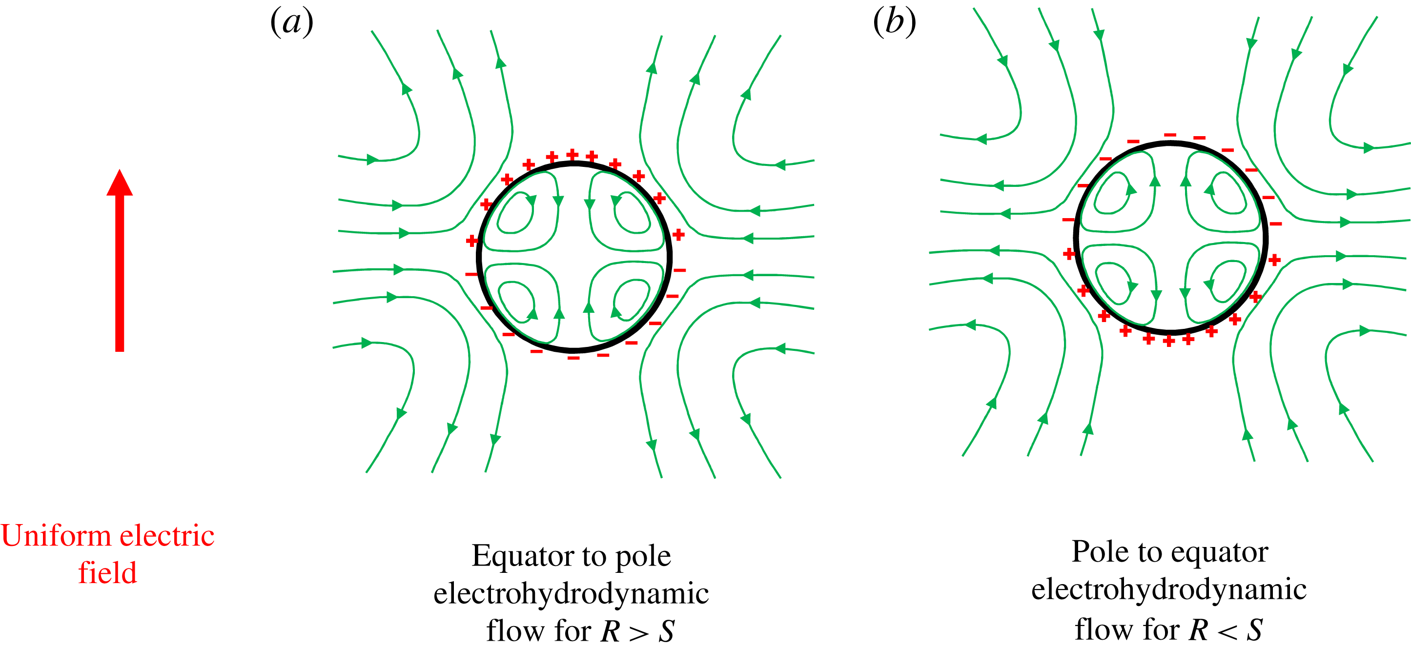
). As the charges at each pole encounter the opposite charges of the nearby electrode (e.g. the upper hemisphere encounters the negative electrode), the charges at each pole will be attracted by the nearby electrode. This attraction causes a jump in tangential electric traction which drives an EHD flow from the equator towards the poles (refer to figure 8
a). The physical situation is reversed for
 $R<S$
as depicted in figure 8(b). For
 $R<S$
or equivalently
 $t_{e}<t_{i}$
the ohmic conduction in the suspending phase is much faster (due to the small time scale) than the ohmic conduction in drop phase. Consequence of this is the charging of the drop surface by the bulk charges coming from the suspending phase. In the presence of a uniform electric field acting along the positive
 $z$
direction, the fast conduction in the suspending phase leads to accumulation of negative charges at the upper hemispherical surface (
 $0\leqslant \unicode[STIX]{x1D703}<\unicode[STIX]{x03C0}/2$
), while positive charges accumulate at the lower hemispherical surface (
 $\unicode[STIX]{x03C0}/2<\unicode[STIX]{x1D703}\leqslant \unicode[STIX]{x03C0}$
). As the charges at each pole encounter similar charges of the nearby electrode, the charges at each pole will be repelled by the nearby electrode. This repulsion causes a jump in tangential electric traction which drives an EHD flow from the poles towards the equator (refer to figure 8
b).
(a) Variation of surface charge distribution over the drop interface for
 $R=2$
,
 $S=0.5$
,
 $\unicode[STIX]{x1D706}=0.1$
and
 $M=3$
. (b) Variation of surface charge distribution over the drop interface for
 $R=0.1$
,
 $S=2$
,
 $\unicode[STIX]{x1D706}=0.1$
and
 $M=1$
.

The previously mentioned distribution of surface charges is likely to be disturbed by the extensional and EHD components of fluid flow. The combined influence of the extensional flow and the EHD flow on the charge distribution is governed by
 $R$
,
 $S$
,
 $\unicode[STIX]{x1D706}$
and
 $M$
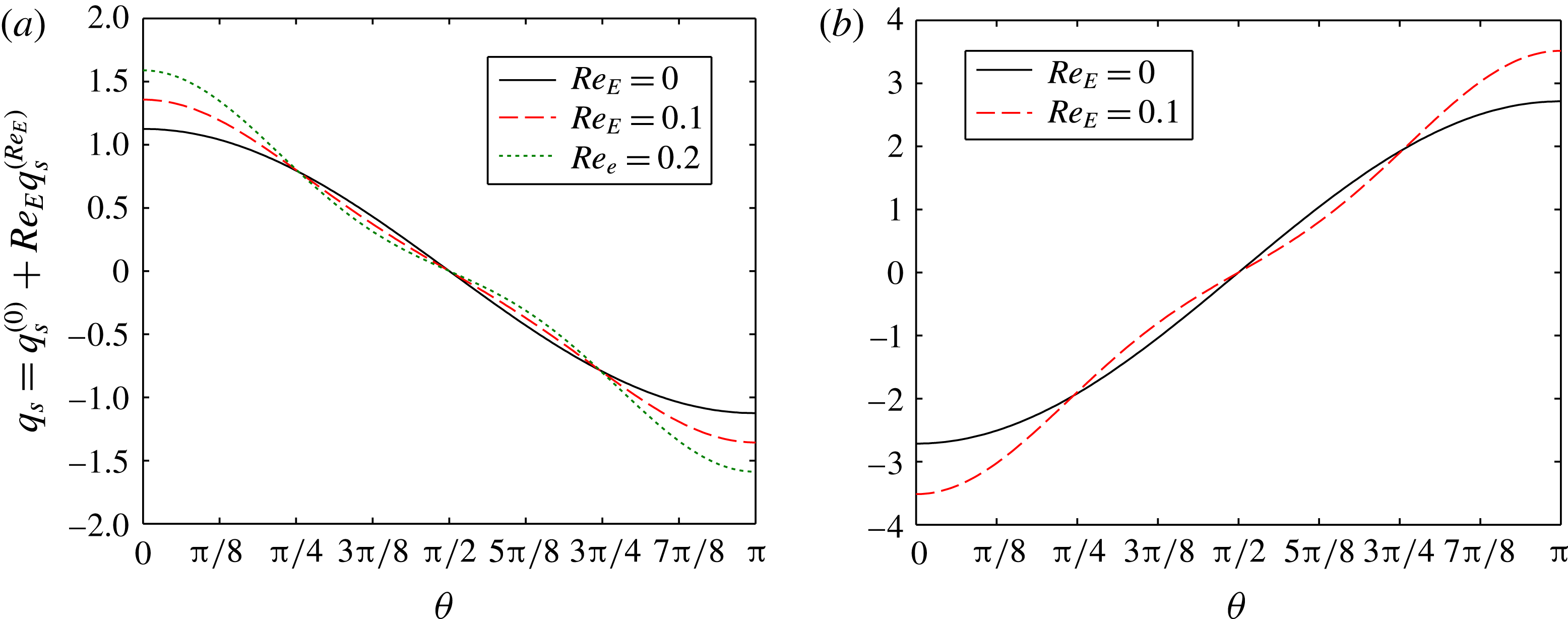
. In figure 9 we show the distribution of surface charges
 $q_{s}=q_{s}^{(0)}+Re_{E}q_{s}^{\left(Re_{E}\right)}$
, where
 $q_{s}^{(0)}$
and
 $q_{s}^{\left(Re_{E}\right)}$
are the leading-order and
 $O(Re_{E})$
charge distributions, respectively. When
 $R>S$
the velocity at the drop surface always runs from the equator to the poles as both the extensional flow and EHD flow act in the same direction. In the presence of surface charge convection (i.e.
 $Re_{E}>0$
), this equator-to-poles surface velocity drives the charges from the equator to the poles which leads to an increase in surface charge density near the poles and decrease in charge density near the equator, as depicted in figure 9(a). As the charges at each pole are attracted by the nearby electrode, the increase in surface charge density near the poles drastically increases the jump in the normal component of electric traction near the poles which finally results in larger drop deformation for
 $Re_{E}>0$
. The increase in the jump of the normal component of electric traction eventually increases the drop deformation because
 $\unicode[STIX]{x1D6FA}_{T}>0$
which means the electric-field-induced deformation (prolate shape) augments the extensional-flow-induced deformation (prolate shape). Thus, for
 $R>S$
the charge convection has a destabilizing effect on the drop shape. Now, we discuss the case of
 $R<S$
for which the velocity at the drop surface can run in either direction (equator to poles or poles to equator) as the extensional flow and EHD flow act opposite to each other. For
 $M=1$
, the extensional flow dominates and the surface velocity runs from the equator to poles. Thus, in the presence of surface charge convection (i.e.
 $Re_{E}>0$
), this equator-to-poles surface velocity drives the charges from the equator to the poles which leads to an increase in surface charge density near poles and a decrease in charge density near the equator as depicted in figure 9(b). As the charges at each pole are repelled by the nearby electrode, the increase in surface charge density near the poles drastically increases the jump in the normal component of electric traction near the poles which finally results in smaller drop deformation for
 $Re_{E}>0$
. The increase in the jump of the normal component of electric traction eventually reduces the drop deformation because
 $\unicode[STIX]{x1D6FA}_{T}<0$
(for
 $(R,S)=(0.1,2)$
) which means the electric-field-induced deformation (oblate shape) opposes the extensional-flow-induced deformation (prolate shape). On the contrary, for
 $M=2$
the charge convection effect increases the drop deformation (as depicted in figure 7
b). This is due to the fact that for
 $M=2$
the EHD flow dominates over the extensional flow and the surface velocity is directed from the poles to the equator. This poles-to-equator flow eventually drives the charges away from the poles and reduces the charge density near the poles. Reduction in surface charge density yields a significant decrease in the jump in the normal component of electric traction which finally results in larger drop deformation for
 $Re_{E}>0$
. Thus, for
 $R<S$
the charge convection has a stabilizing/destabilizing effect on the drop shape.
(a) Variation of drop deformation with capillary number for
 $S=5$
,
 $\unicode[STIX]{x1D706}=1$
and
 $M=2$
. (b) Variation of drop deformation with capillary number for
 $R=0.5$
,
 $S=2$
,
 $\unicode[STIX]{x1D706}=1$
,
 $Re_{E}=0.1$
and
 $M=2$
. Drop shapes (line represent higher-order analytical theory and marker represents numerical) are shown as insets.

5.2.2 Comparison of analytical solution against numerical simulation
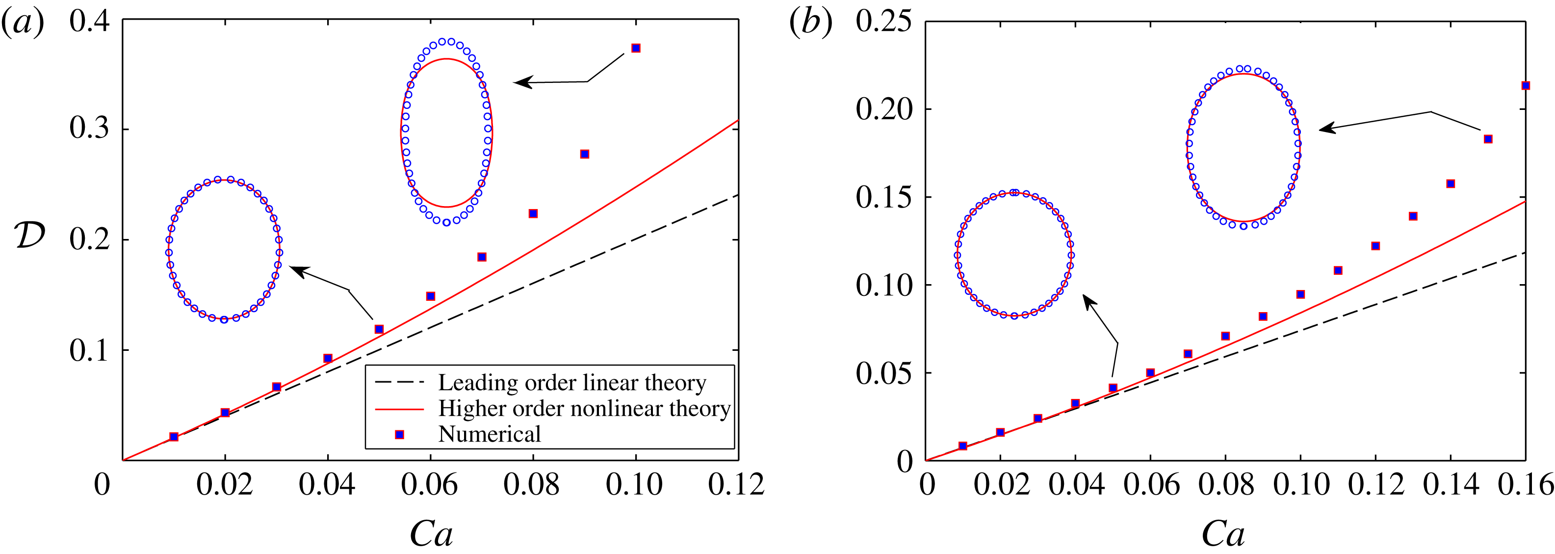
To verify the applicability of the present asymptotic theory in the combined presence of electric field and extensional flow, we compare the analytical results with the results obtained from full-scale numerical simulations. We plot variation of drop deformation with capillary number in figure 10(a) for the PD–PD system with
 $S=5$
, and figure 10(b) for the LD–LD system with
 $(R,S)=(0.5,2)$
. It is evident from these panels that both the leading-order linear theory (i.e. taking only the
 $O(Ca)$
deformation into account) and the higher-order nonlinear theory (i.e. taking
 $O(Ca)$
,
 $O(Ca^{2})$
and
 $O(CaRe_{E})$
deformations into account) compare very well with the numerical solution for small values of Ca. With an increase in Ca, the higher-order nonlinear theory gives a better match with the numerical solution as compared with the leading-order linear theory. Several drop shapes are also shown as insets in figure 10. Analytically obtained drop shapes compare very well with the numerically obtained drop shapes in the small deformation regime. In the large deformation regime, the numerical solution shows more elongated drop shapes which deviate from the analytical solution. Thus the higher-order nonlinear theory under predicts the deformation as we go for larger values of Ca. Important thing to note here is that for the EHD property ratios under consideration, the combination of
 $O(Ca^{2})$
and
 $O(CaRe_{E})$
corrections leads to an increase in deformation which indicates that with an increase in Ca the drop will break eventually. So, higher-order terms have a destabilizing effect on the drop shape.
(a) Variation of drop deformation with Mason number. (b) Variation of semi-major and semi-minor axes of the deformed drop with Mason number for
 $R=2$
and
 $S=0.5$
. Other parameters are taken as for
 $\unicode[STIX]{x1D706}=1$
,
 $Ca=0.05$
and
 $Re_{E}=0.1$
.

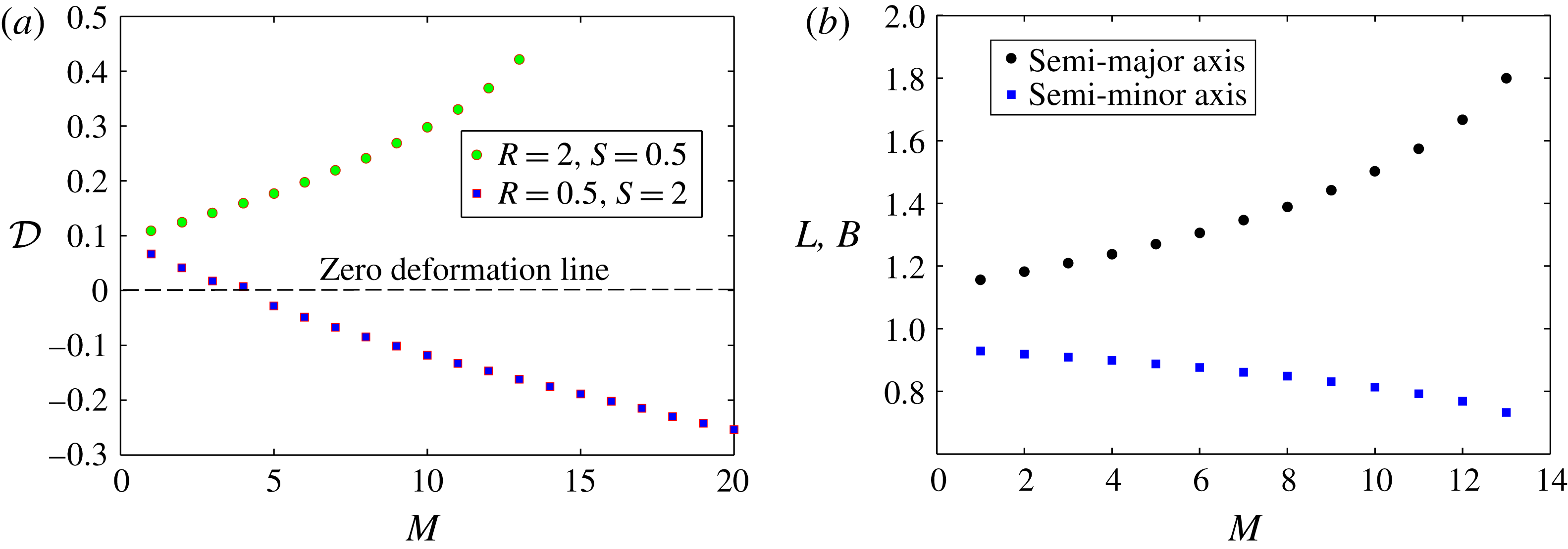
To investigate the drop deformation beyond the small deformation limit, we plot the variation of drop deformation over a wide range of Mason numbers in figure 11(a). As the asymptotic theory is valid for
 $M\sim 1$
, in figure 11(a) we show only numerical results. Also note that the magnitude of the deformation obtained from the numerical simulations (as depicted in figure 11
a) is beyond the regime of validity of asymptotic theory. Figure 11(a) shows that for
 $(R,S)=(2,0.5)$
the drop deforms into a prolate shape for all values of
 $M$
. This is due to the fact that the Taylor discriminating function
 $\unicode[STIX]{x1D6FA}_{T}>0$
which means the uniform electric field aids the drop deformation due to uniaxial extensional flow. Drop deformation significantly increases for larger values of
 $M$
. On the other hand, for
 $(R,S)=(0.5,2)$
we obtain prolate deformation of the drop when
 $M$
is small. But with increase in
 $M$
, the magnitude of drop deformation decreases and eventually the drop deforms into an oblate shape. This prolate-to-oblate shape transition is due to the fact that the Taylor discriminating function
 $\unicode[STIX]{x1D6FA}_{T}<0$
for
 $(R,S)=(0.5,2)$
which means the uniform electric field counteracts the extensional-flow-induced drop deformation. For relatively smaller values of
 $M$
, uniaxial extensional flow dominates and the drop deforms to a prolate shape, while for larger values of
 $M$
the uniform electric field dominates and deforms the drop into an oblate shape. For this case, there is a critical value of
 $M$
for which the deformation is zero which signifies the fact the normal components of hydrodynamic and electric tractions cancel each other. Note that the deformation parameter
 ${\mathcal{D}}$
lumps the two semi-axes in one single parameter. To show the influence of electric field on the individual semi-axes of the drop, we plot the variation of semi-major axis (
 $L$
) and semi-minor axis (
 $B$
) with the Mason number in figure 11(b) for
 $(R,S)=(2,0.5)$
. Note that in the present study two semi-axes are sufficient to describe the drop shape completely because the drop shape is axisymmetric. Figure 11(b) shows that with an increase in Mason number the semi-major axis becomes more elongated, while the semi-minor axis becomes more compressed. This explains the rapid increase in
 ${\mathcal{D}}$
with Mason number shown in figure 11(a). The opposite behaviour of the two semi-axes is due to the fact that the drop volume is conserved. Thus, the decrease in length of the semi-minor axis is always associated with the increase in length of the semi-major axis.
(a) Variation of the normalized leading-order extensional viscosity ratio with viscosity ratio. (b) Variation of the normalized leading-order extensional viscosity ratio with strain rate (
 $M^{-1}$
) for
 $\unicode[STIX]{x1D706}=0.1$
.

5.3 Effect of uniform electric field on the emulsion extensional viscosity
The effective extensional viscosity represents the bulk behaviour of an emulsion in response to a tensile or elongation stress. For a Newtonian fluid the extensional viscosity is three times the shear viscosity (Shroff et al.
Reference Shroff, Cancio and Shida1977). However, this relation does not hold for emulsions. Drops perturb the imposed extensional flow and thereby induce the stresslet tensor and alter the effective extensional viscosity of the emulsion. The electric field affects the extensional viscosity in two different ways: (i) the EHD flow interacts with the extensional flow, and (ii) the electric field deforms the drop. Towards investigating the effect of electric field, we first consider the case in which the drops remain spherical and charge convection is absent. We plot the variation of
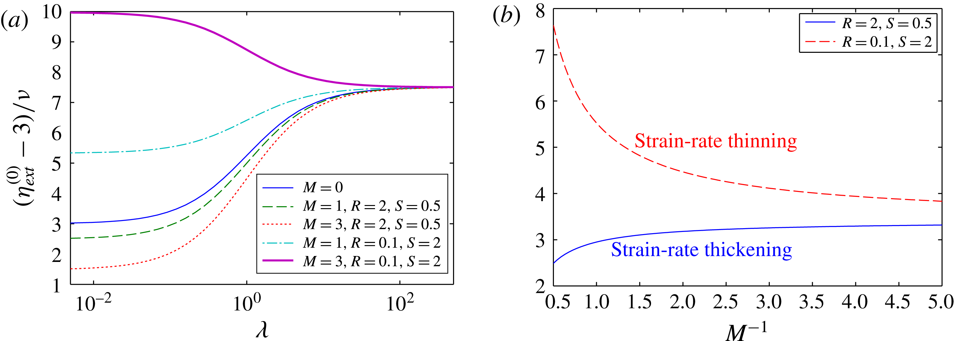
 $(\unicode[STIX]{x1D702}_{ext}^{(0)}-3)/\unicode[STIX]{x1D708}$
in figure 12(a) for two different cases: (i)
 $R>S$
(e.g.
 $R=2$
and
 $S=0.5$
), and (ii)
 $R<S$
(e.g.
 $R=0.5$
and
 $S=2$
). In the absence of an electric field (i.e.
 $M=0$
),
 $\unicode[STIX]{x1D702}_{ext}^{(0)}$
increases with viscosity ratio. This increase in extensional viscosity ratio is attributed to the fact that a highly viscous drop severely decreases the magnitude of the velocity in and around the drop, which further increases the rate of dissipation in the flow. Figure 12(a) shows that application of a uniform electric field significantly decreases (or increases)
 $\unicode[STIX]{x1D702}_{ext}^{(0)}$
when
 $R>S$
(or
 $R<S$
). The physical reason for this increase (or decrease) in
 $\unicode[STIX]{x1D702}_{ext}^{(0)}$
can be found by looking into the nature of the flow field. For
 $R>S$
, the EHD flow runs from equator to poles, which aids the extensional flow and thereby decreases
 $\unicode[STIX]{x1D702}_{ext}^{(0)}$
. On the other hand, for
 $R<S$
the EHD flow runs from poles to equator, which resists the extensional flow and thereby increases
 $\unicode[STIX]{x1D702}_{ext}^{(0)}$
. Another important thing to note from figure 12(a) is that the effect of electric field on
 $\unicode[STIX]{x1D702}_{ext}^{(0)}$
diminishes for larger values of
 $\unicode[STIX]{x1D706}$
. This is attributed to the fact that the EHD flow ceases to exist for larger values of
 $\unicode[STIX]{x1D706}$
. Another important thing to note from figure 12(a) is that a higher value of
 $\unicode[STIX]{x1D706}$
always leads to a higher value of
 $\unicode[STIX]{x1D702}_{ext}^{(0)}$
for
 $R>S$
. This is due to fact that that the velocity at the drop interface runs from equator to poles irrespective of the value of
 $M$
. However, for
 $R<S$
we obtain (i) larger
 $\unicode[STIX]{x1D702}_{ext}^{(0)}$
for larger value of
 $\unicode[STIX]{x1D706}$
when
 $M=1$
, and (ii) larger
 $\unicode[STIX]{x1D702}_{ext}^{(0)}$
for lower value of
 $\unicode[STIX]{x1D706}$
when
 $M=3$
. This is attributed to the fact that for
 $M=1$
the surface velocity is dominated by the imposed extensional flow which yields equator-to-poles flow at the drop interface. On the other hand, for
 $M=3$
the poles-to-equator EHD flow dominates over the extensional flow at the drop interface. This makes larger
 $\unicode[STIX]{x1D702}_{ext}^{(0)}$
for a lower value of
 $\unicode[STIX]{x1D706}$
when
 $M=3$
.
A very interesting point to note from the leading-order extensional viscosity is the strain-rate dependency of the effective viscosity. When the electric field is absent (i.e.
 $M=0$
), it is evident from (3.10) that
 $\unicode[STIX]{x1D702}_{ext}^{(0)}$
is solely a function of viscosity ratio. But when the electric field is present (i.e.
 $M>0$
),
 $\unicode[STIX]{x1D702}_{ext}^{(0)}$
becomes strain-rate dependent because the Mason number (
 $M=\unicode[STIX]{x1D700}_{e}E_{\infty }^{2}/\unicode[STIX]{x1D707}_{e}G$
) is inversely proportional to the strain rate. To show the strain-rate-dependent property of the emulsion, we plot the variation of
 $\unicode[STIX]{x1D702}_{ext}^{(0)}$
with the normalized strain rate (i.e.
 $M^{-1}$
) in figure 12(b). For
 $R>S$
(e.g.
 $R=2$
and
 $S=0.5$
) the extensional viscosity increases with increase in strain rate, while for
 $R<S$
(e.g.
 $R=0.5$
and
 $S=2$
) the extensional viscosity decreases with increase in strain rate. Thus, the emulsion exhibits strain-rate thickening behaviour for
 $R>S$
. The strain-rate thickening behaviour for
 $R>S$
is attributed to the fact that with an increase in strain rate (or decrease in Mason number) the magnitude of the EHD flow reduces. As the EHD flow aids the extensional flow for
 $R>S$
, a decrease in EHD flow effectively increases the resistance to flow and thereby increases the effective viscosity. On the other hand, the emulsion exhibits strain-rate thinning behaviour for
 $R<S$
. The strain-rate thinning behaviour for
 $R<S$
is attributed to the fact that with an increase in strain rate (or decrease in Mason number) the magnitude of the EHD flow reduces. As the EHD flow retards the extensional flow for
 $R<S$
, a decrease in EHD flow effectively decreases the resistance to flow and thereby decreases the effective viscosity.
For the PD–PD system (i.e. when
 $R=S$
) the external electric field has no effect on the leading-order effective extensional viscosity ratio. This is due to the fact that for a PD–PD system the EHD flow vanishes. However, shape deformation can affect the effective extensional viscosity at
 $O(Ca)$
even for the PD–PD system. Shape deformation modifies the distribution of the electric potential and flow field at
 $O(Ca)$
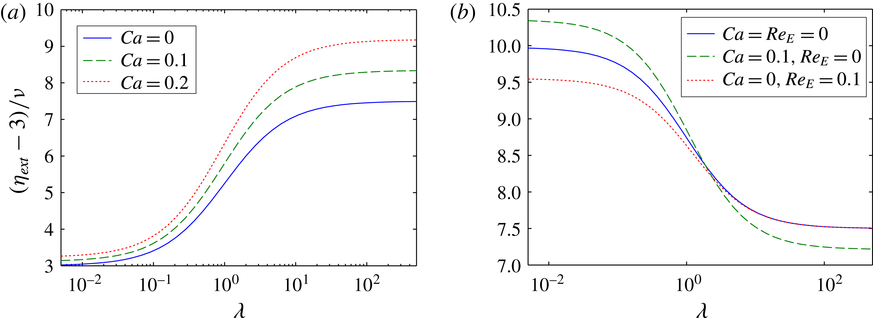
and thereby perturbs the imposed extensional flow. To investigate the effect of shape deformation on the emulsion rheology, we plot the variation of
 $(\unicode[STIX]{x1D702}_{ext}-3)/\unicode[STIX]{x1D708}$
with viscosity ratio for
 $R=S=5$
in figure 13(a). Shape deformation is found to increase the effective extensional viscosity as evident from figure 13(a). This increase in
 $\unicode[STIX]{x1D702}_{ext}$
is attributed to the prolate shape of the drop. As the drops are stretched along the extension axis, the interfacial tension combined with the large curvature near the poles resists any further extension of the fluid element along the extension axis. Thus, a prolate shape is associated with a larger extensional viscosity as compared to a spherical shape. Things become more interesting for the LD–LD system due to the combined presence of shape deformation and charge convection. To investigate the effect of shape deformation and surface charge convection, we plot the variation of
 $(\unicode[STIX]{x1D702}_{ext}-3)/\unicode[STIX]{x1D708}$
with viscosity ratio for
 $(R,S)=(0.1,2)$
in figure 13(b). First we consider the case of a deformable drop with no charge convection (i.e.
 $Ca=0.1$
and
 $Re_{E}=0$
). In this case the shape deformation can increase (or decrease) the effective extensional viscosity for smaller (or larger) values of viscosity ratio. Note that in this case the drop deforms into an oblate shape (considering
 $M=3$
). As the drops are stretched perpendicular to the extension axis, the interfacial tension combined with large curvature near the equator augments any further extension of the fluid element along the extension axis. Thus, an oblate shape is associated with smaller effective extensional viscosity as compared to a spherical shape. But for a LD drop the shape deformation also modifies the EHD flow around the drop, which resists the extensional flow for
 $R<S$
(this is the case under consideration). Thus, the mode of deformation leads to a decrease in effective viscosity, while the EHD flow acts opposite to that of the extensional flow. Therefore, depending on the relative strength of the electric field and extensional flow, either effect can dominate and the extensional viscosity can increase or decrease. In the large viscosity ratio limit, the EHD flow vanishes and the effective viscosity reduces due to the oblate shape. Now, we consider the case of a spherical drop with charge convection (i.e.
 $Ca=0$
and
 $Re_{E}=0.1$
). Charge convection alters the surface charge distribution and creates
 $O$
(
 $Re_{E}$
) electric traction. This electric traction induces a flow which perturbs the imposed extensional flow and thereby modifies the extensional viscosity. In this case charge convection modifies the EHD flow and reduces the effective extensional viscosity. Effect of charge convection vanishes for larger viscosity ratio as the surface velocity vanishes in the limit
 $\unicode[STIX]{x1D706}\rightarrow \infty$
. The combined effect of shape deformation and charge convection can be obtained by linearly combining these two effects which leads to an increase or decrease the effective extensional viscosity depending on the relative magnitude of the electrohydrodynamic parameters.
(a) Variation of the normalized extensional viscosity ratio with viscosity ratio for
 $R=S=5$
and
 $M=1$
. (b) Variation of the normalized extensional viscosity ratio with viscosity ratio for
 $R=0.1$
,
 $S=2$
and
 $M=3$
.

6 Conclusions
In this paper, we have studied the EHD of a drop under the combined influence of a uniform electric field uniaxial extensional flow using both analytical and numerical methods. Considering the capillary number (Ca) and the electric Reynolds number (
 $Re_{E}$
) as small parameters, we have performed an asymptotic analysis and obtained an analytical expression for the drop deformation parameter correct up to
 $O(Ca^{2})$
and
 $O(CaRe_{E})$
. Numerical calculations were performed for small to large values of the governing parameters. An analytical solution is also obtained for the effective extensional viscosity of a dilute suspension of drops. After studying the effect of different governing parameters on the drop deformation and emulsion rheology, the following important conclusions can be drawn:
(i) Irrespective of the value of
 $S$
(except
 $S=1$
), the deformation of a perfectly dielectric drop in the combined presence of a uniform electric field and uniaxial extensional flow always deforms into a prolate shape. The magnitude of deformation is larger than either the electric-field-induced deformation or extensional-flow-induced deformation.
(ii) The deformation of a leaky dielectric drop in the combined presence of a uniform electric field and uniaxial extensional flow depends on the values of
 $\unicode[STIX]{x1D6FA}_{T}$
(
 $R,S,\unicode[STIX]{x1D706}$
) and
 $M$
. When
 $\unicode[STIX]{x1D6FA}_{T}>0$
, both electric field and extensional flow attempt to deform the drop into a prolate shape and the drop always attains a prolate shape. The drop deformation is larger as compared with either electric-field-induced or extensional-flow-induced drop deformation. When
 $\unicode[STIX]{x1D6FA}_{T}<0$
, the electric field tries to deform the drop into an oblate shape, while extensional flow always tries to deform the drop into a prolate shape. Depending on the values of the EHD property ratios and
 $M$
, the drop can attain a prolate/oblate shape with larger/smaller drop deformation.
(iii) Charge convection at the drop surface is found to increase the drop deformation for
 $R>S$
, while charge convection can increase/decrease the drop deformation for
 $R<S$
depending on the value of
 $M$
.
(iv) Analytical solution for drop deformation compares well with the numerical solution when Ca and
 $Re_{E}$
are small. Numerical solution obtained for large values of
 $M$
shows significant stretching of the semi-major axis.
(v) In the presence of a uniform electric field, the effective extensional viscosity becomes strain-rate dependent. The EHD flow leads to smaller (or larger) effective extensional viscosity for
 $R>S$
(or
 $R<S$
) as compared with the case of no electric field. The dilute emulsion exhibits strain-rate thickening (or thinning) behaviour for
 $R>S$
(or
 $R<S$
). Shape deformation always leads to an increase in effective extensional viscosity for a perfectly dielectric drop, while for a leaky dielectric drop the effective extensional viscosity can increase/decrease due to the combined effect of shape deformation and surface charge convection.
The present study effectively establishes the fact that the drop deformation in the combined presence of a uniform electric field and uniaxial extensional flow is not a mere linear superposition of electric-field-induced and extensional-flow-induced drop deformations. The analytical solution unveils the controlling parameters which govern the drop shape, magnitude of deformation and the suspension rheology.
Supplementary material
Supplementary material is available at https://doi.org/10.1017/jfm.2017.897.
Appendix A. Perfectly dielectric system and its relation to leaky dielectric system
A perfectly dielectric fluid does not contain any charge. Thus, under the paradigm of a perfectly dielectric model, the electrostatic problem is governed by the Laplace equation for electric potential in the following form
 $$\begin{eqnarray}\displaystyle \unicode[STIX]{x1D6FB}^{2}\unicode[STIX]{x1D711}_{i}=0,\quad \unicode[STIX]{x1D6FB}^{2}\unicode[STIX]{x1D711}_{e}=0. & & \displaystyle\end{eqnarray}$$
At the drop interface, the electric potential is continuous
 $$\begin{eqnarray}\displaystyle \unicode[STIX]{x1D711}_{i}=\unicode[STIX]{x1D711}_{e}\quad \text{at }r=r_{s}\left(\unicode[STIX]{x1D703}\right). & & \displaystyle\end{eqnarray}$$
In sharp contrast to the leaky dielectric model, the normal component of the electric displacement is continuous at the drop interface
 $$\begin{eqnarray}\displaystyle \boldsymbol{n}\boldsymbol{\cdot }\boldsymbol{D}_{i}=\boldsymbol{n}\boldsymbol{\cdot }\boldsymbol{D}_{e}\quad \text{at }r=r_{s}(\unicode[STIX]{x1D703}), & & \displaystyle\end{eqnarray}$$
where
 $\boldsymbol{D}_{i}=-S\unicode[STIX]{x1D735}\unicode[STIX]{x1D711}_{i}$
and
 $\boldsymbol{D}_{e}=-\unicode[STIX]{x1D735}\unicode[STIX]{x1D711}_{e}$
are the electric displacement inside and outside the drop, respectively. A direct comparison between (A1) and (2.2) shows that the governing equations of the leaky dielectric model and the perfectly dielectric model are identical. The same is also true for the potential continuity condition at the drop interface. Now, we recall the charging condition at the drop interface for the leaky dielectric model in the limit
 $R=S$
as
 $$\begin{eqnarray}\displaystyle \boldsymbol{n}\boldsymbol{\cdot }\left(S\unicode[STIX]{x1D735}\unicode[STIX]{x1D711}_{i}-\unicode[STIX]{x1D735}\unicode[STIX]{x1D711}_{e}\right)=-Re_{E}\unicode[STIX]{x1D735}_{s}\boldsymbol{\cdot }\left(q_{s}\boldsymbol{V}_{s}\right)\quad \text{at }r=r_{s}\left(\unicode[STIX]{x1D703}\right). & & \displaystyle\end{eqnarray}$$
Note that the surface charge density in the limit
 $R=S$
vanishes (i.e.
 $q_{s}=0$
), which further simplifies equation (A 4) to
 $$\begin{eqnarray}\displaystyle \boldsymbol{n}\boldsymbol{\cdot }\left(S\unicode[STIX]{x1D735}\unicode[STIX]{x1D711}_{i}-\unicode[STIX]{x1D735}\unicode[STIX]{x1D711}_{e}\right)=0\quad \text{at }r=r_{s}\left(\unicode[STIX]{x1D703}\right). & & \displaystyle\end{eqnarray}$$
A direct comparison between (A 3) and (A 5) shows that the normal component of the electric displacement is continuous for both the perfectly dielectric model and the leaky dielectric model when
 $R=S$
. The vanishing surface charge density,
 $q_{s}=0$
, can be explained in terms of the charge relaxation time scale and its relation to the
 $R/S$
ratio. The charge relation time scale (
 $t=\unicode[STIX]{x1D700}/\unicode[STIX]{x1D70E}$
) signifies the time required for the charges to reach steady state. Note that
 $R/S=(\unicode[STIX]{x1D70E}_{i}/\unicode[STIX]{x1D70E}_{e})/(\unicode[STIX]{x1D700}_{i}/\unicode[STIX]{x1D700}_{e})=(\unicode[STIX]{x1D700}_{e}/\unicode[STIX]{x1D70E}_{e})/(\unicode[STIX]{x1D700}_{i}/\unicode[STIX]{x1D70E}_{i})$
represents the ratio of charge relation time scale of the suspending phase (
 $t_{e}=\unicode[STIX]{x1D700}_{e}/\unicode[STIX]{x1D70E}_{e}$
) to the charge relaxation time scale of the drop phase (
 $t_{i}=\unicode[STIX]{x1D700}_{i}/\unicode[STIX]{x1D70E}_{i}$
). For a leaky dielectric system, the net charges contained in the drop phase and suspending phase are independently zero. However, due to the small conductivity of the fluid, equal amounts of positive and negative charges are present in drop phase as well as in the suspending phase. The limit
 $R=S$
signifies that the charge relaxation time scale of the drop phase is the same as the charge relation time scale of suspending phase. This physically means that the charges from both the drop phase and suspending phase will come to the interface of the leaky dielectric drop at the same time, which finally leads to vanishing surface charge density (Salipante & Vlahovska Reference Salipante and Vlahovska2010).
Appendix B. Complete expression of different terms
Different terms appearing in (3.4) and (3.6) are obtained as
 $$\begin{eqnarray}\displaystyle \ell _{1} & = & \displaystyle \frac{9}{3500}\frac{\left(\begin{array}{@{}l@{}}1730R+726R^{2}+680S+800\unicode[STIX]{x1D706}+920+519\unicode[STIX]{x1D706}R^{2}\\ +920S\unicode[STIX]{x1D706}+1340\unicode[STIX]{x1D706}R+564SR+726SR\unicode[STIX]{x1D706}\\ \end{array}\right)\left(\begin{array}{@{}l@{}}20+20R+5R^{2}\\ +6MR-6MS\\ \end{array}\right)}{\left(\unicode[STIX]{x1D706}+1\right)\left(4+3R\right)\left(\unicode[STIX]{x1D706}R^{2}+R^{2}+4\unicode[STIX]{x1D706}R+4R+4\unicode[STIX]{x1D706}+4\right)\left(2+R\right)^{3}},\nonumber\\ \displaystyle & & \displaystyle\end{eqnarray}$$
 $$\begin{eqnarray}\displaystyle \ell _{2} & = & \displaystyle \frac{2}{175}\frac{\left(33\unicode[STIX]{x1D706}R+96S-20+36R-16\unicode[STIX]{x1D706}+102S\unicode[STIX]{x1D706}\right)\left(20+20R+5R^{2}+6MR-6MS\right)}{\left(4+3R\right)\left(\unicode[STIX]{x1D706}+1\right)\left(\unicode[STIX]{x1D706}R^{2}+R^{2}+4\unicode[STIX]{x1D706}R+4R+4\unicode[STIX]{x1D706}+4\right)\left(2+R\right)^{2}},\nonumber\\ \displaystyle & & \displaystyle\end{eqnarray}$$
 $$\begin{eqnarray}\displaystyle \ell _{3} & = & \displaystyle \frac{9}{700}\frac{\left\{\begin{array}{@{}l@{}}\left(\begin{array}{@{}l@{}}638MS+280-68MR-240M+210R^{2}\\ +420R+35R^{3}-479MSR+90MR^{3}+59MR^{2}\\ \end{array}\right)\unicode[STIX]{x1D706}^{2}\\ +\left(\begin{array}{@{}l@{}}-811MSR+5R^{3}+30R^{2}-480M-178MR\\ +40+60R+1318MS-29MR^{2}+180MR^{3}\\ \end{array}\right)\unicode[STIX]{x1D706}\\ +\left(\begin{array}{@{}l@{}}-320+90MR^{3}-320MSR-240R^{2}+704MS\\ -240M-40R^{3}-100MR^{2}-480R-134MR\\ \end{array}\right)\\ \end{array}\right\}}{\left(R+2\right)^{3}\left(\unicode[STIX]{x1D706}+1\right)^{2}},\end{eqnarray}$$
 $$\begin{eqnarray}\displaystyle \ell _{4} & = & \displaystyle \frac{\left\{\begin{array}{@{}l@{}}\left(500R^{3}+4000+6000R+3000R^{2}\right)\unicode[STIX]{x1D706}^{2}\\ +\left(12000R+1000R^{3}+6000R^{2}+8000\right)\unicode[STIX]{x1D706}\\ +\left(500R^{3}+4000+6000R+3000R^{2}\right)\\ \end{array}\right\}}{700\left(R+2\right)^{3}\left(\unicode[STIX]{x1D706}+1\right)^{2}},\end{eqnarray}$$
 $$\begin{eqnarray}\displaystyle \ell _{5} & = & \displaystyle \frac{\left\{\begin{array}{@{}l@{}}\left(4660R+1165R^{2}+360MR^{2}+4660+678MR-1398MS+360M\right)\unicode[STIX]{x1D706}\\ +\left(528MR-1248MS+4160+360MR^{2}+4160R+1040R^{2}+360M\right)\\ \end{array}\right\}}{1050\left(R+2\right)^{2}\left(\unicode[STIX]{x1D706}+1\right)},\end{eqnarray}$$
 $$\begin{eqnarray}\displaystyle \ell _{6} & = & \displaystyle \frac{1200\unicode[STIX]{x1D706}+1200+1200\unicode[STIX]{x1D706}R+1200R+300\unicode[STIX]{x1D706}R^{2}+300R^{2}}{1050\left(R+2\right)^{2}\left(1+\unicode[STIX]{x1D706}\right)}.\end{eqnarray}$$