2 Set-up and results from direct numerical simulations

In this study, we consider forced incompressible 3-D flow in a triply periodic domain of dimensions $L\times L\times H$ with $H\ll L$ . The set-up is identical with the one studied in van Kan & Alexakis (Reference van Kan and Alexakis2019). The thin direction is referred to as the vertical ‘ $z$ ’ direction and the remaining two as the horizontal ‘ $x,y$ ’ directions. The flow obeys the incompressible Navier–Stokes equation

where $\boldsymbol{v}(\boldsymbol{x},t)$ is the velocity field, $P(\boldsymbol{x},t)$ is the physical pressure divided by constant density, $\unicode[STIX]{x1D708}$ is the kinematic viscosity and $\boldsymbol{f}$ is the external body force injecting energy into the flow. In this work, we use two different forcing functions: stochastic $\boldsymbol{f}_{s}$ and deterministic $\boldsymbol{f}_{d}$ . Both forcing functions depend only on $x$ and $y$ and have only $x$ and $y$ components, i.e. are two-dimensional-two-component (2D2C) fields. In both cases, the force is divergence free and only acts on a shell of wavenumbers $|\boldsymbol{k}|=k_{f}=2\unicode[STIX]{x03C0}/\ell$ . The stochastic force is delta correlated in time, which leads to a fixed mean injection rate $\langle \boldsymbol{v}\boldsymbol{\cdot }\,\boldsymbol{f}_{\boldsymbol{s}}\rangle =\unicode[STIX]{x1D716}$ . The deterministic force $\boldsymbol{f}_{d}$ is written in terms of the Fourier transform of the velocity field, $\hat{\boldsymbol{v}}(\boldsymbol{k})$ , as

where the sums are taken over all modes in the set $K_{F}$ that consists of all wavenumbers with $k_{z}=0$ and $k_{f}\leqslant |\boldsymbol{k}|<k_{f}+1$ and only in-plane components $\hat{\boldsymbol{v}}_{\mathit{2}\text{-}D}=(\hat{v}_{x},\hat{v}_{y},0)$ are forced. There are two terms in this forcing. The first term is responsible for injecting energy at a fixed rate $\unicode[STIX]{x1D716}$ , matching the mean injection rate of $\boldsymbol{f}_{s}$ . The second term is not injecting energy, but is responsible for de-correlating the phases of the forced modes at a time scale given by $(\unicode[STIX]{x1D716}k_{f}^{2})^{-1/3}$ . This is achieved by the linear term $i(\unicode[STIX]{x1D716}k_{f}^{2})^{1/3}\unicode[STIX]{x1D6FA}_{\boldsymbol{k}}\hat{\boldsymbol{v}}(\boldsymbol{k})$ where $\unicode[STIX]{x1D6FA}_{\boldsymbol{k}}$ are time-independent random numbers that are uniformly distributed over $[-1,1]$ . They are kept fixed throughout the simulation time and are the same for all simulations. Since $\unicode[STIX]{x1D6FA}_{\boldsymbol{k}}$ are time independent, the forcing is indeed deterministic, i.e. is fully determined by the velocity field at any time. Without the second term, the flow at late times is attracted to a degenerate state where the velocity and the forcing are strongly correlated so that two strong vortices with opposite signs, of the size of the forcing scale, are formed. This forcing (2.2) has previously been used successfully by Benavides & Alexakis (Reference Benavides and Alexakis2017).

For both forcing functions, the system is characterised by three non-dimensional parameters: the injection-scale Reynolds number $Re=(\unicode[STIX]{x1D716}\ell ^{4})^{1/3}/\unicode[STIX]{x1D708}$ , the ratio between forcing scale and box height $Q=\ell /H$ and the ratio between forcing scale and the horizontal domain size $K=\ell /L$ . In all simulations, we focus on the horizontal large-scale kinetic energy, defined as

where $k_{max}=\sqrt{2}(2\unicode[STIX]{x03C0}/L)$ . The simulations performed for this work use an adapted version of the Geophysical High-Order Suite for Turbulence (GHOST) which uses pseudo-spectral methods including $2/3$ de-aliasing to solve for the flow in the triply periodic domain (see Mininni et al. Reference Mininni, Rosenberg, Reddy and Pouquet2011). For all experiments, we fix $K=1/8$ and $Re=203$ at a resolution of $128\times 128\times 16$ , varying $Q$ over the interval $[1.4,2.0]$ . We choose this low resolution and $Re$ because very long-duration runs are needed for this study. In addition, we also made runs at a resolution $256\times 256\times 16$ at $Re=406$ , which qualitatively showed the same dynamics, even though reliable statistical analysis was not done in this case due to the longer CPU times required to integrate (2.1).

Figure 1.

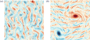
Top view of the flow field visualised in terms of vorticity (positive in red, negative in blue) in 3-D flow state (a) and 2-D condensate state (b). Both snapshots are taken for stochastic forcing at $Q=1.56$ , approximately in the middle of the hysteresis loop.

Figure 2.

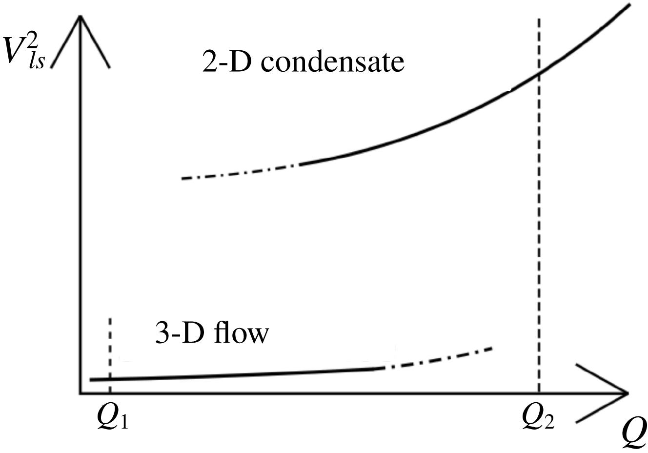
Sketch illustrating the hysteresis loop close to the critical height. Solid and dash-dotted lines represent the stable and unstable branches. We select initial conditions for decay and build-up experiments from the typical configurations at sufficiently small and large values of $Q$ (here denoted by $Q_{1}$ and $Q_{2}$ ), respectively.

Depending on $Q$ and the initial conditions, the system is attracted either to the 2-D condensate state or the 3-D flow state. Two snapshots of the vorticity for these two states are displayed in figure 1 where in (a) the flow is in the 3-D state and has a small value of $V_{ls}$ while in (b) the flow is in the 2-D condensate state and has large value of $V_{ls}$ . Figure 2 shows a sketch of these states in the $Q{-}V_{ls}$ plane. The upper branch corresponds to the 2-D condensate state while the lower branch corresponds to the 3-D flow state. The dash-dotted lines indicate regions where one of the two states is unstable and the flow can jump from that state to the other. As detailed below, we perform decay and build-up experiments for each value of $Q$ . In the build-up experiments, initial conditions corresponding to the 3-D flow state are used (see figure 2). In these simulations, we observe the build-up of 2-D condensates after a certain simulation time, which we denote by $\unicode[STIX]{x1D70F}_{b}$ . In the decay experiments, initial conditions corresponding to the 2-D condensate state are used. The system is evolved until the 2-D condensate decays, where the decay time is denoted by $\unicode[STIX]{x1D70F}_{d}$ . 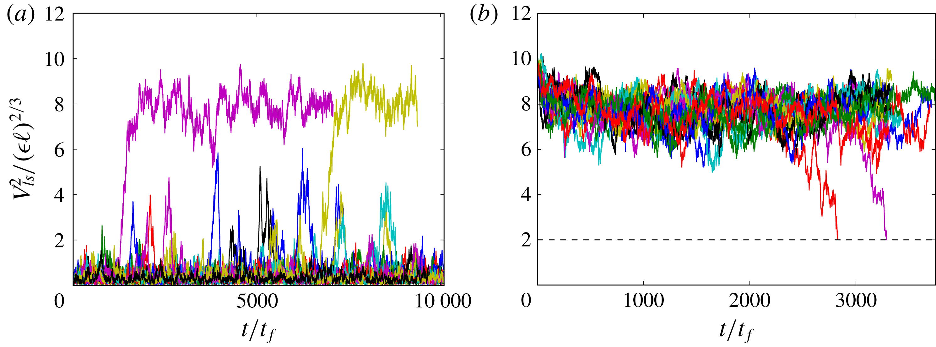When decay or build-up events occur, the integration is interrupted and the next independent experiment is initiated. For the stochastic forcing, runs are started from a fixed initial condition but with different random number sequences, while for deterministic forcing, the initial conditions are altered by a small random perturbation that is different for every run. Figure 3 illustrates typical time series for build-up and decay experiments. We note that similar procedures have been used to determine a critical Reynolds number for turbulent–laminar transitions in pipe flows (see Avila et al. Reference Avila, Moxey, de Lozar, Avila, Barkley and Hof2011).

Figure 3.

Typical time series of $V_{ls}^{2}$ for build-up experiments ( $Q=1.55$ , a) and decay ( $Q=1.556$ , b) experiments ( $\,\boldsymbol{f}=\boldsymbol{f}_{s}$ ). We define a build-up time $\unicode[STIX]{x1D70F}_{b}$ (or a decay time $\unicode[STIX]{x1D70F}_{d}$ ) as the time when $V_{ls}^{2}$ grows (or drops) to its condensate mean value (or a small threshold ${\approx}2(\unicode[STIX]{x1D716}\ell )^{2/3}$ ). These $\unicode[STIX]{x1D70F}_{b}$ and $\unicode[STIX]{x1D70F}_{d}$ fluctuate and their statistics are of our interest.

Figure 4.

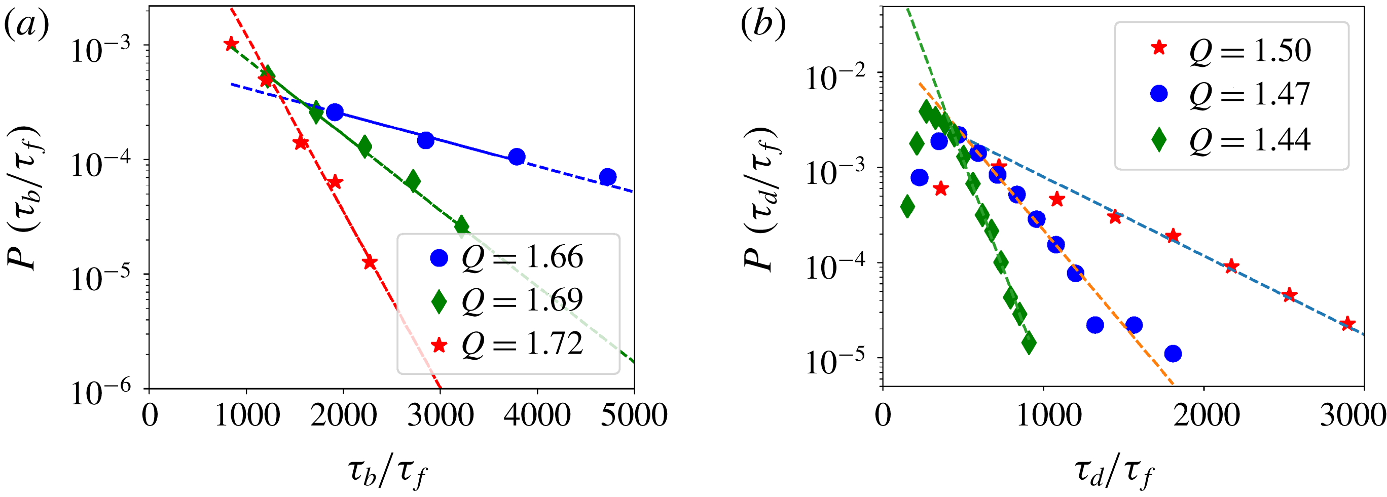
PDFs of the scaled build-up time $\unicode[STIX]{x1D70F}_{b}/\unicode[STIX]{x1D70F}_{f}$  (a) and the scaled decay time $\unicode[STIX]{x1D70F}_{d}/\unicode[STIX]{x1D70F}_{f}$  (b) for different values of $Q$ , with $\unicode[STIX]{x1D70F}_{f}=(\ell ^{2}/\unicode[STIX]{x1D716})^{1/3}$ . The stochastic forcing $\boldsymbol{f}_{s}$ is used. The PDFs have exponential tails whose characteristic time scale increases as the transition is approached.

3 Build-up and decay times

We measure the statistical properties of the decay and build-up times $\unicode[STIX]{x1D70F}_{d},\unicode[STIX]{x1D70F}_{b}$ by simulating the system for more than ten million ( $10^{7}$ ) eddy turnover times, using a total of 2.5 million CPU hours. This corresponds to between 40 and over 1000 independent runs per value of $Q$ . Figure 4 shows PDFs of $\unicode[STIX]{x1D70F}_{d}$ and $\unicode[STIX]{x1D70F}_{b}$ for the stochastic forcing $\boldsymbol{f}_{s}$ for different values of $Q$ . All PDFs have an exponential tail, whose slope (in log–linear scale) increases as the transition is approached. The PDFs for the deterministic forcing $\boldsymbol{f}_{d}$ show qualitatively the same results. The PDFs remain almost unchanged when half of the data points in the sample are removed, which indicates that they are sufficiently well sampled. An exponential PDF of waiting times implies that the waiting mechanism can be modelled using a memoryless process, in which long-time correlations are absent (Billingsley Reference Billingsley2008). We explore this possibility in § 4.

Figure 5.

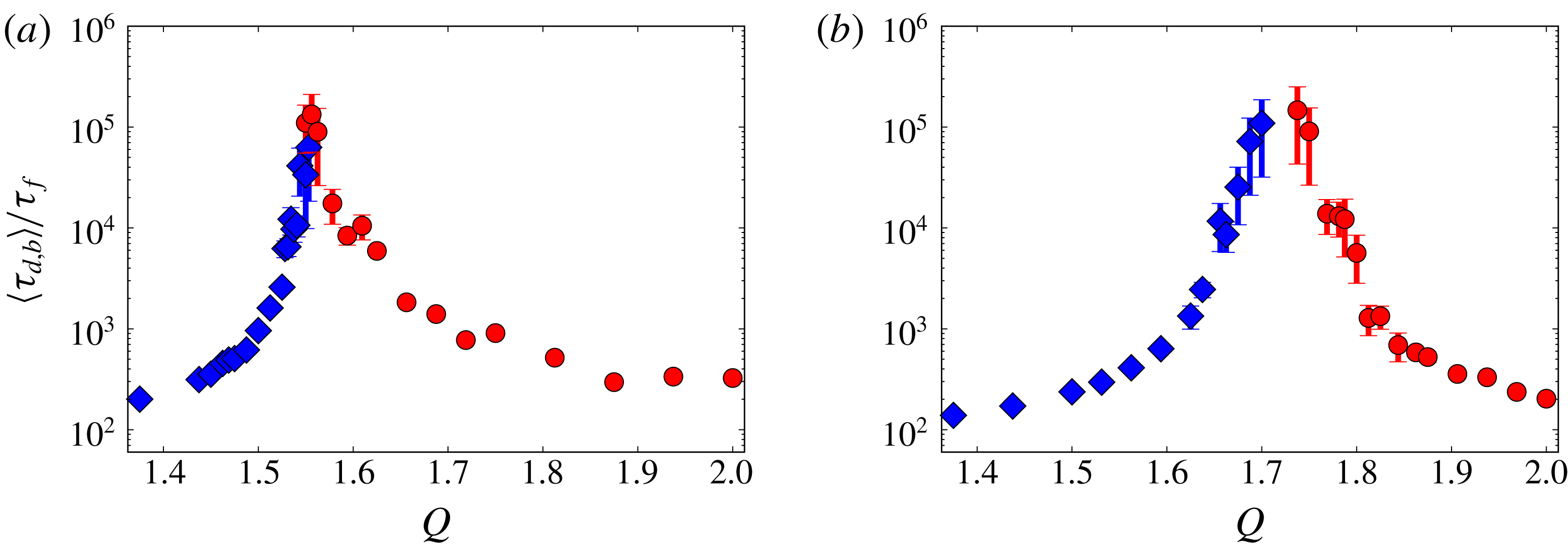
Mean transition times, non-dimensionalised by $\unicode[STIX]{x1D70F}_{f}=(\ell ^{2}/\unicode[STIX]{x1D716})^{1/3}$ , for stochastic (a) and deterministic (b) forcing as a function of $Q$ . Blue diamonds correspond to $\langle \unicode[STIX]{x1D70F}_{d}\rangle$ in the decay experiments and red circles correspond to $\langle \unicode[STIX]{x1D70F}_{b}\rangle$ in the build-up experiments. Error bars are estimated based on the approximation that the PDF is exactly exponential.

The resulting mean build-up and decay times, $\langle \unicode[STIX]{x1D70F}_{b}\rangle ,\langle \unicode[STIX]{x1D70F}_{d}\rangle$ , are shown in figure 5 for stochastic (a) and deterministic (b) forcing in log–linear coordinates. The uncertainty in the transition times due to the finite sample size is estimated based on exponential PDFs and shown by the error bars. The ascending branch (left, in blue) represents the mean decay time $\langle \unicode[STIX]{x1D70F}_{d}\rangle$ and the descending branch (right, in red) represents the build-up time $\langle \unicode[STIX]{x1D70F}_{b}\rangle$ . For each case, both transition times increase drastically when a certain value of $Q$ is approached. This increase is faster than exponential (super-exponential) and could be either diverging at some critical values $Q_{b}$ and $Q_{d}$ or staying finite (similar to what is observed for the decay and split time of turbulent puffs in pipe flows (Hof et al. Reference Hof, Westerweel, Schneider and Eckhardt2006, Reference Hof, de Lozar, Kuik and Westerweel2008; Avila et al. Reference Avila, Moxey, de Lozar, Avila, Barkley and Hof2011)). In the former case, where the two times diverge, for $Q<Q_{b}$ the 2-D condensate will eventually decay to the 3-D flow state, while for $Q>Q_{d}$ the 3-D state will transition to a condensate. Thus $Q_{d}$ corresponds to the smallest value of $Q$ for which a condensate can be observed at late times, while $Q_{b}$ is the largest value of $Q$ at which a 3-D flow state can be observed. Both $Q_{b}$ and $Q_{d}$ are close to the value $Q_{\mathit{3}\text{-}D}\propto 1/H_{_{\mathit{3}\text{-}D}}$ that gives the onset of the inverse cascade as observed in Benavides & Alexakis (Reference Benavides and Alexakis2017) and van Kan & Alexakis (Reference van Kan and Alexakis2019). We note however that in Benavides & Alexakis (Reference Benavides and Alexakis2017), where the presence of a hypo-viscosity and the large box limit was considered, no bistability was observed, while in van Kan & Alexakis (Reference van Kan and Alexakis2019) due to the limited statistics in that work the distinction between $Q_{b}$ and $Q_{d}$ could not be made. In the latter case where transition times stay finite despite the super-exponential increase, a double-exponential function might be used to fit this super-exponential increase, supported by an argument using extreme value statistics (Fisher & Tippett Reference Fisher and Tippett1928; Gumbel Reference Gumbel1935; Goldenfeld, Guttenberg & Gioia Reference Goldenfeld, Guttenberg and Gioia2010; Goldenfeld & Shih Reference Goldenfeld and Shih2017). This can be justified if we assume that the transition to the condensate state is triggered when the maximum value of the small-scale vorticity exceeds a certain threshold value. Testing this assumption requires knowledge of the entire flow field at times near rare transition events. We believe that it would be important to clarify this question in a future study.

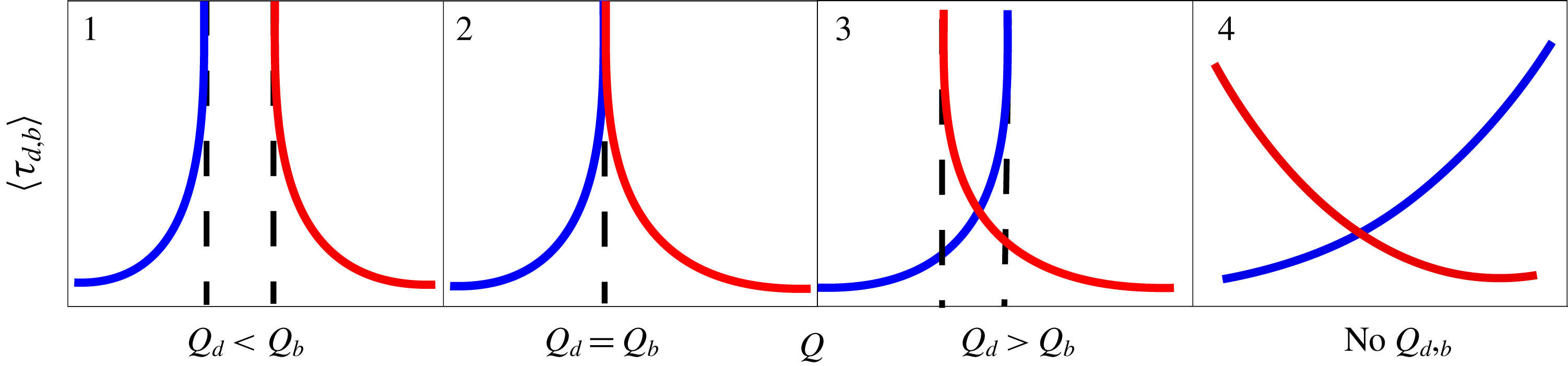
Four different scenarios may be envisaged for the $Q$ -dependence of the transition times, illustrated in figure 6. In the first scenario, both $\langle \unicode[STIX]{x1D70F}_{b}\rangle$ and $\langle \unicode[STIX]{x1D70F}_{d}\rangle$ diverge at $Q_{b},Q_{d}$ with $Q_{d}<Q_{b}$ . In the range $(Q_{d},Q_{b})$ , where both transition times diverge, either the 3-D flow or 2-D condensate state is selected, depending on the initial conditions. In the second scenario, $\langle \unicode[STIX]{x1D70F}_{b}\rangle$ and $\langle \unicode[STIX]{x1D70F}_{d}\rangle$ diverge at the same point, i.e.  $Q_{d}=Q_{b}$ . This is an analogue of standard equilibrium phase transitions with a single power-law singularity. In the third scenario, a cross-over is observed, i.e.  $Q_{b}<Q_{d}$ , where random transitions between the two states are possible within a finite range of $Q$ between $Q_{b}$ and $Q_{d}$ . Finally, in the fourth scenario, a cross-over is again observed, but without any divergence of $\langle \unicode[STIX]{x1D70F}_{b}\rangle$ and $\langle \unicode[STIX]{x1D70F}_{d}\rangle$ for finite $Q$ . This scenario is compatible with the double-exponential fitting function explained above, where transitions between the two states are possible for all $Q$ (although they are extremely rare). From the data in figure 5, we can see that for the stochastic forcing, the two branches intersect around $Q=Q_{s}\approx 1.55$ at a value of approximately $10^{5}$ eddy turnover times. Therefore, we can exclude cases 1 and 2 for $\boldsymbol{f}_{s}$ , while all four scenarios are possible for $\boldsymbol{f}_{d}$ . In addition, it may be proven (see Gallet & Doering Reference Gallet and Doering2015) and has been confirmed numerically (van Kan & Alexakis Reference van Kan and Alexakis2019), that beyond a second critical value $Q_{\mathit{2}\text{-}D}$ , the flow two-dimensionalises and the condensate is stable to 3-D perturbations in the long-time limit. Therefore, condensate decay time diverges at least for $Q>Q_{\mathit{2}\text{-}D}$ and we can exclude a double-exponential behaviour extending to all $Q$ for $\langle \unicode[STIX]{x1D70F}_{d}\rangle$ . Note that based on our available data, we cannot exclude that condensate build-up time never becomes infinite. In a future study, rare event algorithms (see § 5) may help elucidating these questions, including the problem of how rare transitions are triggered.

An alternative way of reducing the computational cost of the problem could be to consider not the statistics of transition events which become extremely rare, but rather the statistics of bursting events, which can be seen in figure 3 to be significantly more frequent than transition events in the bistable regime. While we have not studied them in very much detail, we have found that waiting times for bursting events also follow exponential PDFs, whose mean increases towards larger $Q$ . Bursting events may prove more fruitful than transition events at higher Reynolds numbers and we believe they are a promising object of study for future work.

Figure 6.

Four scenarios for dependence of transition times on $Q$ . In each panel, the $x$ -axis represents $Q$ and the $y$ -axis is either the mean decay time $\langle \unicode[STIX]{x1D70F}_{d}\rangle$ (left branch) or the mean build-up time $\langle \unicode[STIX]{x1D70F}_{b}\rangle$ (right branch). Dashed vertical lines indicate $Q_{d,b}$ , where the mean transition times diverge.

4 Effective Markovian modelling

The exponential PDFs of the transition times (figure 4) indicate that these times are stochastically determined by a mechanism that is memoryless, in other words, which leads to vanishing long-time correlations for these times. Since the transitions are quantitatively characterised by a single macroscopic variable, the horizontal large-scale kinetic energy $V_{ls}^{2}$ (figure 3), this observation implies that the dynamics of $V_{ls}^{2}$ could be described by a Markov (memoryless) process, such as an inertialess particle moving in a double-well potential in the presence of white noise. Within this effective description, the transitions are characterised as rare jumps of the particle between the two wells of the potential.

Motivated by this observation, in this section, we discuss to what extent the dynamics of $E\equiv V_{ls}^{2}/(\unicode[STIX]{x1D716}\ell )^{2/3}$ can be described by a one-dimensional Markov process. Assuming the continuity of the trajectory of $E(t)$ , a general form of this process is written as the following Langevin equation (Gardiner Reference Gardiner1986): denoting by $\unicode[STIX]{x0394}E(t)$ the increment of $E(t)$ during a small time interval $\unicode[STIX]{x0394}t$ , the equation is written as

where $\unicode[STIX]{x0394}W(t)$ is a Gaussian noise satisfying $\langle \unicode[STIX]{x0394}W(t)\rangle =0$ and $\langle \unicode[STIX]{x0394}W(t)\unicode[STIX]{x0394}W(t^{\prime })\rangle =\unicode[STIX]{x0394}t\unicode[STIX]{x1D6FF}_{t,t^{\prime }}$ and we use the Itô rule for the multiplication between $\unicode[STIX]{x0394}W(t)$ and $\sqrt{2B(E)}$ , i.e.  $\langle \sqrt{2B(E)}\unicode[STIX]{x0394}W(t)\rangle =0$ . The potential $U(E)$ and the $E$ -dependent diffusion constant $B(E)$ characterise the dynamics and are to be determined. Note that the noise term models the smaller-scale turbulent motions. Equation (4.1) indicates that the average and the variance of $\unicode[STIX]{x0394}E(t)$ conditional on $E$ are equal to $-(\unicode[STIX]{x2202}U(E)/\unicode[STIX]{x2202}E)\unicode[STIX]{x0394}t$ and $2B(E)\unicode[STIX]{x0394}t$ respectively. 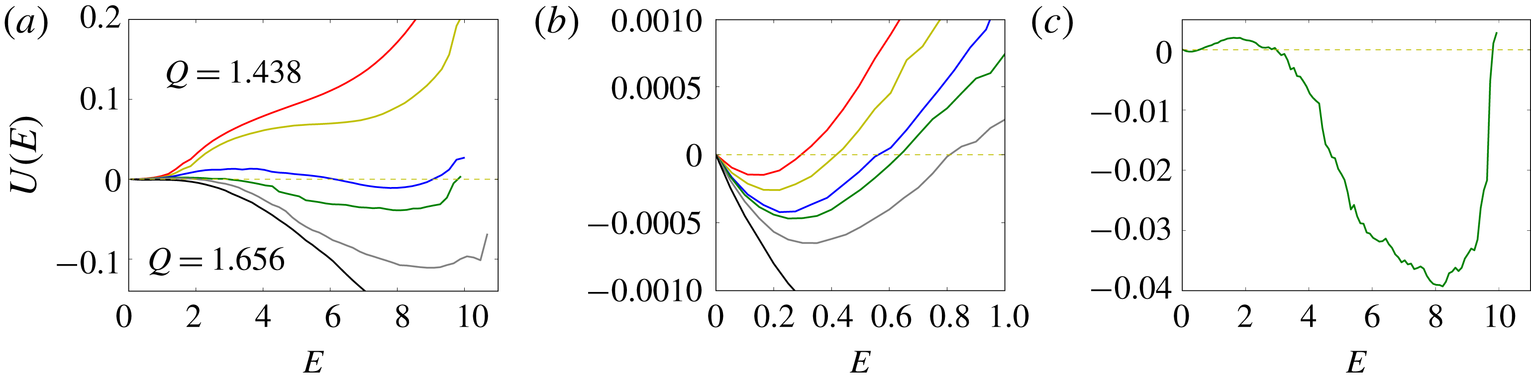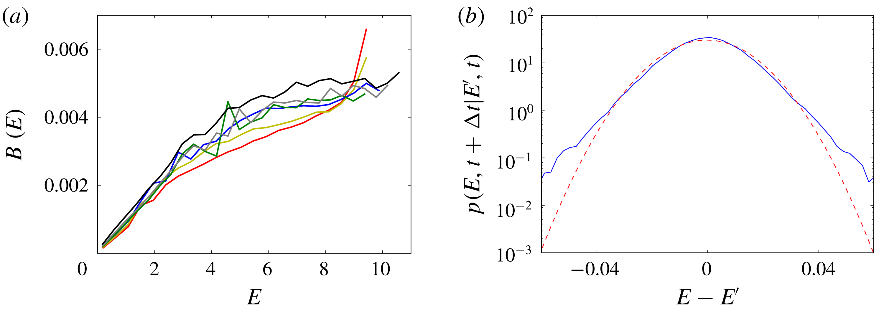From the time-series data of the DNS, we thus evaluate these statistical properties and estimate $U(E)$ and $B(E)$ (see appendix A for more detail). The results are shown in figures 7 and 8. When $Q$ is well below the transition, $U(E)$ has a single minimum at $E\simeq 0.1$ . Positive slopes at larger values of $E$ indicate a mean drift towards the 3-D flow state. As $Q$ approaches the transition, $U(E)$ becomes flatter, meaning that this drift vanishes, and a second minimum appears at $E\simeq 7$ for $Q\simeq 1.5$ . This indicates that the system is in a bistable regime. The second minimum becomes more pronounced as $Q$ is further increased. Eventually, for $Q\gtrsim 1.65$ , the first minimum disappears and the system is left with a single minimum corresponding to the condensate state. The time scale for the system to jump from one minimum to the other can be estimated using a first-passage time formula in terms of $U(E)$ and $B(E)$ (see § 5.2.7 ‘First Passage Times for Homogeneous Processes’ in Gardiner (Reference Gardiner1986)). For example, we consider a transition time for build-up events at $Q=1.563$ , where the corresponding $U(x)$ and $B(x)$ are shown in figure 7(c) and in figure 8(a), respectively. The build-up event is then characterised as the jump from the potential (local) minimum around $E_{min}=0.3$ to the potential maximum around $E_{max}=1.8$ . In this range of $E$ , $B(E)$ can be well described as a linear function $B(E)=bE$ (with $b\simeq 0.001$ ). We also approximate $U(E)$ as a linear function $U(E)=aE+c$ (with $a\simeq 0.002$ ) for simplicity. (A generalisation for more realistic potentials is straightforward (Gardiner Reference Gardiner1986). Here we choose this approximation because the obtained formula (4.2) becomes simple.) Using the first-passage time formula we get the time scale $\unicode[STIX]{x1D70F}_{b}$ as

which estimates $\unicode[STIX]{x1D70F}_{b}=2\times 10^{4}$ . This shows a rough agreement with the data in figure 5(a) in the previous section. (We set a reflecting boundary at $E=E_{min}$ and an absorbing boundary at $E=E_{max}$ . Substituting the explicit expressions of $B(E)$ and $U(E)$ into the mean first-passage time formula on p.139 of Gardiner (Reference Gardiner1986), we get (4.2). Note that, for a more detailed analysis, we need to model $B(E)$ and $U(E)$ outside $E_{min}<E<E_{max}$ , and define a reflecting boundary at $E=0$ and an absorbing boundary at another local minimum of $U(E)$ corresponding to the 2-D stable state. This will possibly increase the estimation of $\unicode[STIX]{x1D70F}_{b}$ compared with (4.2).)

Figure 7.

(a) The potential $U(E)$ obtained from DNS (both decay and build-up experiments) for different values of $Q$ . The values of $Q$ from top to bottom are $1.438$ (red), $1.5$ (yellow), $1.556$ (blue), $1.563$ (green), $1.594$ (grey), $1.656$ (black). (b) An enlarged view close to $E=0$ . (c) An enlarged view of $U(E)$ for $Q=1.563$ . The potential is obtained using (A 2) for stochastic forcing.

Figure 8.

(a) The $E$ -dependent diffusion constant $B(E)$ obtained using (A 3) for stochastic forcing. Colours are as in figure 7. (b) Transition probability $p(E,t+\unicode[STIX]{x0394}t|E^{\prime },t)$ obtained from DNS (blue solid line) and a Gaussian fit (red dashed line). We set $E^{\prime }=0.5$ and $\unicode[STIX]{x0394}t=0.2$ with $Q=1.563$ for a stochastic forcing build-up experiment.

The interpretation of our results using a Langevin equation with a double-well potential is the simplest model to describe a discontinuous phase transition. The presence of a double-well potential implies that the system can always jump from one state to the other if one waits long enough. However, we cannot conclude that $\langle \unicode[STIX]{x1D70F}_{d}\rangle$ and $\langle \unicode[STIX]{x1D70F}_{b}\rangle$ do not diverge for finite $Q$ (scenario 4 in figure 6) from this observation. First of all, the range of $Q$ that we have studied is highly limited. Second, an oversimplification has been made when we assumed that the system could be described by a single variable $E$ , while the system in reality evolves in an extremely high-dimensional space. Indeed, disagreements between the 1-D model (4.1) and DNS results can be detected when we look at the distribution of the energy increment $\unicode[STIX]{x0394}E$ over a small time interval $\unicode[STIX]{x0394}t$ . According to the Langevin equation (4.1), this distribution needs to be Gaussian, but this is not exactly true for the DNS results: using the time-series data of DNS, we evaluate the transition probability $p(E,t+\unicode[STIX]{x0394}t|E^{\prime },t)$ from the state $E^{\prime }$ at time $t$ to $E$ at time $t+\unicode[STIX]{x0394}t$ . In figure 8 we plot this probability with $E^{\prime }=0.5$ and $\unicode[STIX]{x0394}t=0.2$ for stochastic forcing with $Q=1.5625$ , showing deviations from a Gaussian distribution.