1 Introduction
Magnetic fluids are colloidal liquids in which magnetic nanoparticles are suspended within non-magnetic carrier fluids. Such magnetic fluids combine fluidity with magnetic properties, and have thus attracted numerous investigations by scholars and engineers in the fields of sealing, interfacial instability, micromixers, natural convection and even biomolecule selection (Rosensweig Reference Rosensweig1997; Chen & Wen Reference Chen and Wen2002; Wen & Su Reference Wen and Su2005; Wen et al. Reference Wen, Yeh, Tsai and Fu2009, Reference Wen, Lin, Chen, Chen and Liang2011; Lai & Hong Reference Lai and Hong2014). Accordingly, the patterns of interfacial instability in magnetic fluids have been investigated intensively. One remarkable type of pattern is associated with the so-called labyrinthine instability, in which highly branched structures are formed when a magnetic drop is confined in a Hele-Shaw cell and subjected to a perpendicular external field (Cēbers & Maiorov Reference Cēbers and Maiorov1980a ,Reference Cēbers and Maiorov b ; Langer, Goldstein & Jackson Reference Langer, Goldstein and Jackson1992; Dickstein et al. Reference Dickstein, Erramilli, Goldstein, Jackson and Langer1993; Jackson, Goldstein & Cēbers Reference Jackson, Goldstein and Cēbers1994; Flament et al. Reference Flament, Pacitto, Bacri, Drikis and Cēbers1998; Cēbers & Drikis Reference Cēbers and Drikis1999; Chen & Wu Reference Chen and Wu2005). When magnetic fluids are confined in a Hele-Shaw cell with a narrow gap between two parallel plates under a normal external magnetic field, the repelling interaction of the magnetic dipolar moments becomes much more significant and induces labyrinthine instabilities in the interfacial regions.
Early investigations concentrated mostly upon the well-defined immiscible interfaces between magnetic and non-magnetic fluids. Promising theoretical and experimental studies on relevant mechanisms at the immiscible interfaces showed the significance of the ratio of the magnetic force to the surface tension, the magnetic Bond number
 $Bo$
(
 $Bo\equiv 2M^{2}h/\unicode[STIX]{x1D70E}$
) and the dimensionless gap span
 $\unicode[STIX]{x1D6EC}$
(
 $\unicode[STIX]{x1D6EC}\equiv h/d$
) (Langer et al.
Reference Langer, Goldstein and Jackson1992; Dickstein et al.
Reference Dickstein, Erramilli, Goldstein, Jackson and Langer1993; Jackson et al.
Reference Jackson, Goldstein and Cēbers1994; Flament et al.
Reference Flament, Pacitto, Bacri, Drikis and Cēbers1998; Cēbers & Drikis Reference Cēbers and Drikis1999; Wen et al.
Reference Wen, Chen, Tsai and Kuan2005; Wen, Chen & Kuan Reference Wen, Chen and Kuan2007a
), where
 $M$
is the magnetisation of the magnetic fluids,
 $\unicode[STIX]{x1D70E}$
is the surface tension,
 $h$
is the cell gap span and
 $d$
is the droplet diameter. Unlike the immiscible situation, labyrinthine instabilities at a miscible interface are dominated by a diffusion effect instead of by interfacial surface tension. Theoretical analysis and numerical simulations have been intensively used to discern its mechanism (Chen & Wen Reference Chen and Wen2002; Chen Reference Chen2003; Igonin & Cēbers Reference Igonin and Cēbers2003; Chen & Liu Reference Chen and Liu2005; Chen & Wu Reference Chen and Wu2005; Chen, Wu & Hsu Reference Chen, Wu and Hsu2005; Wen et al.
Reference Wen, Chen and Kuan2007a
; Ērglis et al.
Reference Ērglis, Tatulcenkov, Kitenbergs, Petrichenko, Ergin, Watz and Cēbers2013; Kitenbergs et al.
Reference Kitenbergs, Tatulcenkovs, Ērglis, Petrichenko, Perzynski and Cēbers2015). These pioneering studies suggested that the magnetic Péclet number
 $Pe_{m}$
or the magnetic Rayleigh number
 $Ra_{m}$
(the ratio of magnetic-driven advection and diffusion) can characterise the miscible situation accurately. In the linear stability analyses of early studies (Wen et al.
Reference Wen, Chen and Kuan2007a
; Ērglis et al.
Reference Ērglis, Tatulcenkov, Kitenbergs, Petrichenko, Ergin, Watz and Cēbers2013; Kitenbergs et al.
Reference Kitenbergs, Tatulcenkovs, Ērglis, Petrichenko, Perzynski and Cēbers2015), a parallel was established between approaches based on Darcy’s law and those based on the Brinkman equations. Chen & Wen (Reference Chen and Wen2002) investigated miscible flows and numerically revealed that a magnetic circular drop in a Hele-Shaw cell would extend fingerings outward and could be strengthened by higher-intensity magnetic parameters and viscous contrast.
Another interesting and important phenomenon associated with the instabilities at a miscible interface in a Hele-Shaw cell is wavelength selection. Many theoretical, numerical and experimental results for viscous fingering instabilities in various flow situations have been reported (Fernandez et al.
Reference Fernandez, Kurowski, Petitjeans and Meiburg2002; Wen et al.
Reference Wen, Chen and Kuan2007a
; Ērglis et al.
Reference Ērglis, Tatulcenkov, Kitenbergs, Petrichenko, Ergin, Watz and Cēbers2013; Kitenbergs et al.
Reference Kitenbergs, Tatulcenkovs, Ērglis, Petrichenko, Perzynski and Cēbers2015; Chen et al.
Reference Chen, Chen, Li and Wen2017). These studies have shown that, for a sufficiently high
 $Pe_{m}$
or
 $Ra_{m}$
, (1) the wavenumber (or wavelength) depends greatly upon the gap span and (2) the conventional Hele-Shaw equations, which apply the averaging velocities across the gap, fail to describe the complete instability phenomena. Under these conditions, solutions of the full three-dimensional Stokes equations or Brinkman equations are required to accurately resolve the complete interfacial evolution. Fernandez et al. (Reference Fernandez, Kurowski, Petitjeans and Meiburg2002) referred to this high-
 $Pe_{m}$
flow condition as the Stokes regime. In general, the wavelength of the miscible fingers has a nearly linear correlation with the gap span
 $h$
in this Stokes regime.
For example, (1) in the experimental study of Paterson (Reference Paterson1985), a source flow of less-viscous fluids was placed at the origin of the cell and displaced the surrounding viscous fluids outwardly,
 $\unicode[STIX]{x1D706}\sim 4h$
, (2) in the downward miscible displacement experiments of Lajeunesse et al. (Reference Lajeunesse, Martin, Rakotomalala and Salin1997), a lighter and less-viscous fluid flow was introduced from the top in a vertical Hele-Shaw cell configuration,
 $\unicode[STIX]{x1D706}\sim (5\pm 1)h$
, and (3) for a gravity-driven flow,
 $\unicode[STIX]{x1D706}\sim 2.3h$
was obtained in an analytical study by Fernandez et al. (Reference Fernandez, Kurowski, Limat and Petitjeans2001), which agrees closely with the experimental result of
 $\unicode[STIX]{x1D706}\sim (5\pm 1)h$
(Fernandez et al.
Reference Fernandez, Kurowski, Petitjeans and Meiburg2002). In contrast, in the situation of a low
 $Pe$
or
 $Ra$
, the conventional Hele-Shaw model is sufficient to resolve the interfacial instability. Therefore, it is referred as the Hele-Shaw regime by Fernandez et al. (Reference Fernandez, Kurowski, Petitjeans and Meiburg2002). In this regime,
 $\unicode[STIX]{x1D706}$
decreases monotonically as
 $Pe_{m}$
or
 $Ra_{m}$
increases and approaches its corresponding asymptotic value in the Stokes regime.
Wen et al. (Reference Wen, Chen and Kuan2007a
) also conducted a series of systematic experiments under constant external magnetic fields which first revealed the formation of a secondary wave of miscible magnetic fluids, caused by the three-dimensional factor of the gap span
 $h$
, which had never been observed or simulated. This study confirmed the defects of the conventional two-dimension theoretical model, which did not consider the gap span
 $h$
. In addition, Wen et al. (Reference Wen, Chen, Kuan and Wu2007b
) observed that the interfacial length grew continuously in the early phase of the process but began to decline when the magnetic field reached the pre-set value, which was consistent with reported observations (Ērglis et al.
Reference Ērglis, Tatulcenkov, Kitenbergs, Petrichenko, Ergin, Watz and Cēbers2013; Kitenbergs et al.
Reference Kitenbergs, Tatulcenkovs, Ērglis, Petrichenko, Perzynski and Cēbers2015). Ērglis et al. (Reference Ērglis, Tatulcenkov, Kitenbergs, Petrichenko, Ergin, Watz and Cēbers2013) found the importance of gravity on the labyrinthine instabilities within a Hele-Shaw cell even when the gap span was
 $127~\unicode[STIX]{x03BC}\text{m}$
. The same group (Kitenbergs et al.
Reference Kitenbergs, Tatulcenkovs, Ērglis, Petrichenko, Perzynski and Cēbers2015) further numerically discovered that the Brinkman model describes the labyrinthine instabilities more accurately than Darcy’s law and shows good agreement with experimental data. These studies have unveiled the significance of the three-dimensional nature of the Hele-Shaw cell experimentally and theoretically, but the mechanism of secondary wave formation in miscible magnetic flows still unclear.
Most magnetic fluid studies have focused on steady cases in which the magnetic field strength is constant at the beginning. Due to the inevitable rising period for any magnetic field generator, a steady magnetic field can be regarded as an increasing magnetic field with an infinite sweep rate (
 $SR=\text{d}H_{t}/\text{d}t\rightarrow \infty$
, where
 $H_{t}$
is the instant magnetic field strength) and requires an infinitesimal period to reach the pre-set magnetic field strength
 $H$
. Similarly, a system without a magnetic field can be regarded as an increasing magnetic field, but the sweep rate is infinitesimal (
 $SR\rightarrow 0$
) so that the magnetic field remains absent. Therefore, a magnetic field with a finite sweep rate (i.e. greater than zero) is interesting for further study and may be related to the formation of secondary waves.
Wen et al. (Reference Wen, Lin, Chen, Chen and Liang2011) investigated the effects of finite
 $SR$
on the labyrinthine instabilities of miscible magnetic fluids in a Hele-Shaw cell with a 1 mm gap span. The growth rate in the early phase was linear in proportion to
 $SR^{1/2}$
and
 $h^{3/2}$
. Due to the limited range of the modified Péclect number, which is introduced in a later section, the initial growth period of interest may not illustrate the full picture of morphological evolution. Secondary waves were detected in their study, but detailed investigations on the mechanism of secondary wave formation were not conducted. Based on the pioneering studies of Fernandez et al. (Reference Fernandez, Kurowski, Petitjeans and Meiburg2002) and Wen et al. (Reference Wen, Chen and Kuan2007a
), secondary wave formation may also undergo a transition when the range of the dependent modified Péclect number is sufficiently large.
In this study, a comprehensive experimental analysis was conducted to extend the previous work of this research group (Wen et al.
Reference Wen, Chen and Kuan2007a
, Reference Wen, Lin, Chen, Chen and Liang2011) to a much larger parameter space by combining variation of the magnetic fluids, the gap span (
 $h$
) and the sweep rates of the external magnetic fields (
 $SR$
) for the miscible labyrinthine instabilities of magnetic flows in a Hele-Shaw cell. Many more data and a larger experimental range are provided here than in previous studies. Competition among four parameters regarding their effects on the labyrinthine and secondary wave instabilities will be investigated in detail. The experimental set-up and material specifications are described in § 2. Section 3 includes the flow visualisation of magnetic fluids in a Hele-Shaw cell and an analysis of the morphological patterns under different experimental conditions, such as the maximum pre-set magnetic field (
 $H$
), the sweep rate (
 $SR$
) and the magnetic fluid samples. In § 4.1, the interfacial length of the magnetic drop is quantified and the initial growth rate is analysed, and the gap effect is also added for analysis. In § 4.2, the initial growth rate is correlated with a modified Péclect number, and so is the ratio of the wavelength and the gap span in § 4.3. Finally, conclusions from the investigation are drawn in § 5.
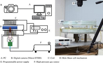
The experimental apparatus consists mainly of a Hele-Shaw cell and a pair of Helmholtz coils to produce a uniform and perpendicular magnetic field. The magnetic fluids and surrounding fluids are all confined within the Hele-Shaw cell.

2 Experimental set-up
The experimental apparatus set-up in this study is shown in figure 1 and is modified from that used by Wen et al. (Reference Wen, Chen and Kuan2007a
). Two parallel plates are used for the Hele-Shaw cell configuration with a narrow gap formed by
 $h$
-mm-thick spacers. The Hele-Shaw cell then confines a magnetic drop with an initial radius (
 $R_{0}$
) of 7.5 mm in the central region, which is surrounded by a miscible non-magnetic fluid (diesel). A pair of Helmholtz coils is designed to generate a magnetic field stabilised at
 $27\,^{\circ }\text{C}$
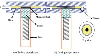
by immersion in a water box. A transparent acrylic plate of the Hele-Shaw cell is chosen for the upper plate with a 10 mm thickness for better visualisation, while the lower plate is an opaque white acrylic plate with a thickness of 14 mm to reinforce the contrast because of the black colour of magnetic fluids. The magnetic field strength is measured with a Gauss meter (Kantec Model TM-701) and adjusted with a programmable power supply (Chroma 6210). For better formation of the circular magnetic drop, a circular groove is created under the surface of the lower plate, as shown in figure 2.
Side views of the Hele-Shaw cell system before and during the experiment. The tube, denoted by the red fringe, works as a divider to isolate the magnetic fluids in the centre and the surrounding diesel, and to sink once the experiments begin. A top view is also displayed on the right.

Because the initial concentration gradient of the mixing interface has been proved to enhance the fingering instabilities Igonin & Cēbers (Reference Igonin and Cēbers2003), a concentration jump of ferrofluids at the mixing front is desired. A mobile circular divider at the centre of the Hele-Shaw cell is therefore designed to close the upper plate from the bottom to form a circular central boundary with a radius (
 $R_{0}$
) of 7.5 mm, initially separating the two sections, which is a similar set-up to that reported in Wen et al. (Reference Wen, Chen and Kuan2007a
). The formation of a circular magnetic drop with initial radius
 $R_{0}$
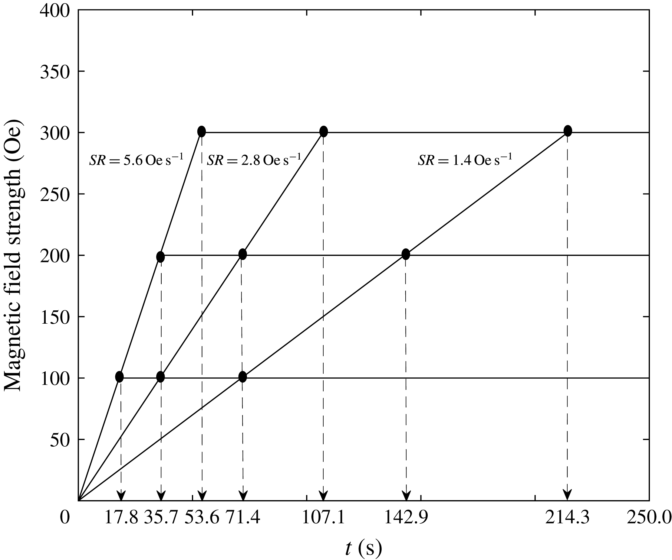
is ensured by injecting magnetic fluids into the inner region of the divider, and the non-magnetic fluid (diesel) is then injected into the outer section. The divider thus prevents premixing before the experiments. The divider can be retracted downward in a precise manner by a pneumatic piston control with a high-pressure gas source (see the green part under the Hele-Shaw cell in figure 1) so that it is located in the plane of the upper surface of the bottom plate. The morphologic features of the magnetic drop are monitored and captured by a Nikon D7000 camera for fingering instability analysis. The initial time (
 $t=0~\text{s}$
) of the experiments is defined as the moment at which the mobile divider sinks. The magnetic field is raised from zero following different sets of maximum magnetic field strengths (
 $H=100,200$
and 300 Oe) and different sweep rates (
 $SR=1.4,2.8$
and
 $5.6~\text{Oe}~\text{s}^{-1}$
), as shown in figure 3, and the sweeping time is defined as the time
 $T$
when the magnetic field grows to its pre-set (
 $H$
), as calculated and listed in table 1.
The nine magnetic field settings in this study are formed by three maximum magnetic field strengths (
 $H=100,200$
and 300 Oe) and three sweep rates (
 $SR=1.4,2.8$
and
 $5.6~\text{Oe}~\text{s}^{-1}$
). The sweeping times,
 $T$
, of the nine magnetic fields are indicated on the
 $t$
-axis by arrows.

The sweeping time (
 $T$
) spent by the different magnetic fields to reach their maximum strength (
 $H$
) with different sweep rates
 $SR$
.

The specifications for the magnetic fluids (EMG905, EMG909 and EMG911) and the diesel. Here,
 $M_{s}$
is the saturation magnetisation,
 $\unicode[STIX]{x1D702}_{m}$
is the viscosity at
 $27\,^{\circ }\text{C}$
, the size is the particle mean radius,
 $\unicode[STIX]{x1D712}$
is the initial susceptibility and
 $\unicode[STIX]{x1D70C}$
is the density.

The magnetic fluids used in the experiments were commercial light hydrocarbon oil-based ferrofluids (EMG905, EMG909 and EMG911) purchased from the Ferrotec Corp. (Tokyo, Japan). Diesel produced by CPC Corp. (Taipei, Taiwan) was chosen as the miscible surrounding fluid due to its miscibility with our chosen magnetic fluids. The specifications for the magnetic fluids and the diesel are listed in table 2, with the viscous Atwood number,
 $At$
, between the magnetic fluid and the diesel. The initial viscous Atwood number is defined as
 $At\equiv (\unicode[STIX]{x1D702}_{m}-\unicode[STIX]{x1D702}_{d})/(\unicode[STIX]{x1D702}_{m}+\unicode[STIX]{x1D702}_{d})$
, where
 $\unicode[STIX]{x1D702}_{m}$
is the initial viscosity of the magnetic fluid and
 $\unicode[STIX]{x1D702}_{d}$
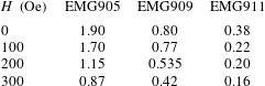
is that of the diesel. In addition, the magnetic susceptibilities corresponding to different magnetic fields are also listed in table 3, as calculated from the magnetisation curves (
 $\unicode[STIX]{x1D712}=M/H$
, where
 $M$
is the magnetisation and
 $H$
is the magnetic field strength) provided by Ferrotec. Therefore, with three different cell gap spans (
 $h=0.8$
, 0.9 and 1.0 mm), our study has 81 sets of data.
The susceptibilities
 $\unicode[STIX]{x1D712}_{H}$
of the various magnetic fluids subjected to different external perpendicular magnetic fields.

3 Experimental visualisation analysis
3.1 Labyrinthine instabilities
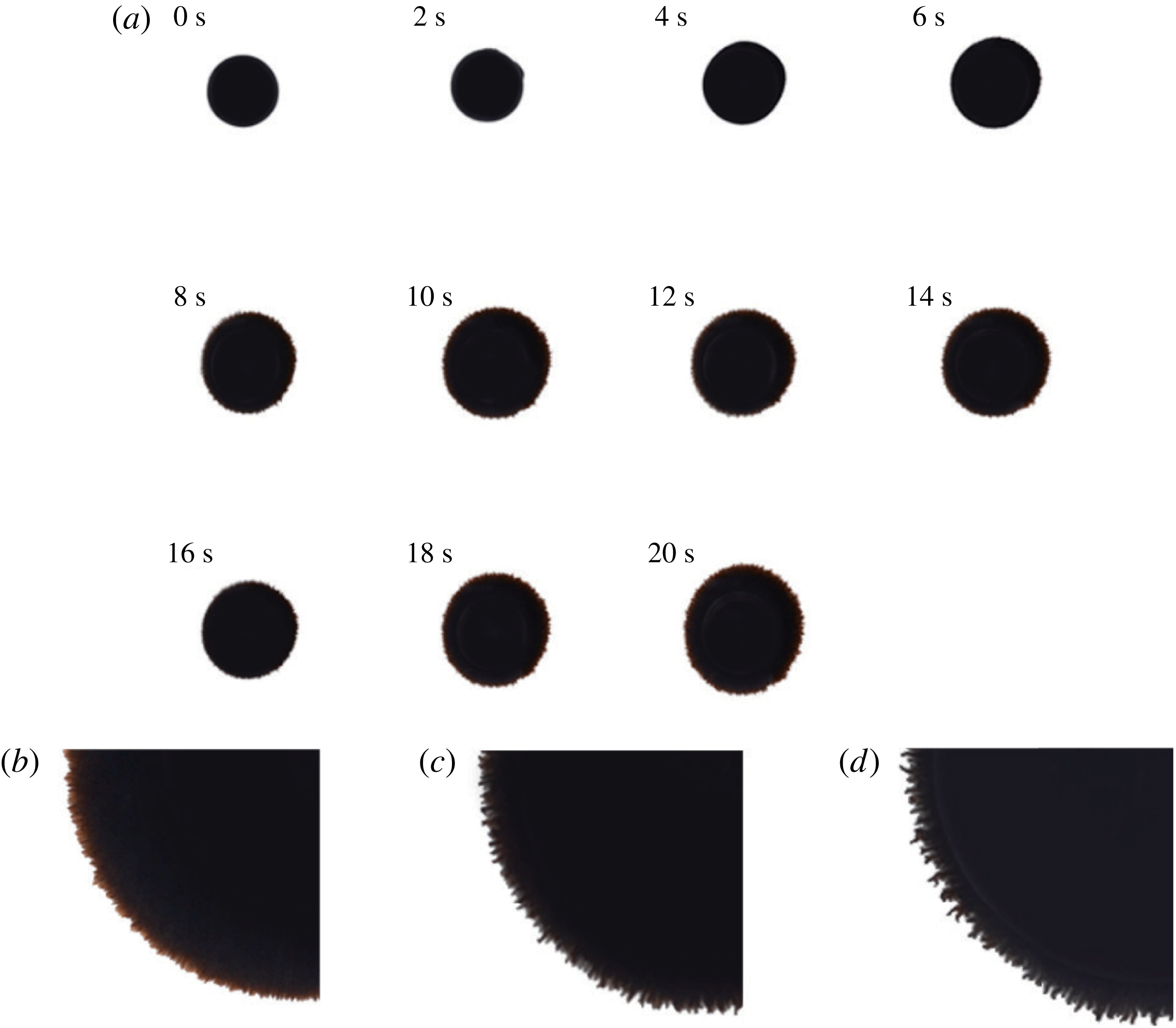
The evolution of instabilities for the early period during which the magnetic field has not reached the pre-set value will be investigated first. A supplementary movie available at https://doi.org/10.1017/jfm.2017.739 demonstrates a clearer picture (see movie 1; experimental conditions:
 $SR=5.6~\text{Oe}~\text{s}^{-1}$
,
 $H=100~\text{Oe}$
, EMG905 and
 $h=1~\text{mm}$
). The smallest pre-set magnetic field strength (
 $H=100~\text{Oe}$
) and fastest sweep rate (
 $SR=5.6~\text{Oe}~\text{s}^{-1}$
) lead to the fastest sweeping time (
 $T=17.8~\text{s}$
). The early period is then defined as before the first 20 s (
 $t\leqslant 20~\text{s}$
). Representative results for the growth for the case with
 $SR=2.8~\text{Oe}~\text{s}^{-1}$
,
 $H=100~\text{Oe}$
and
 $h=1.0~\text{mm}$
are shown in figure 4(a), and the results from other experimental conditions are qualitatively the same. From
 $t=0~\text{s}$
to
 $t=6~\text{s}$
(
 $t\leqslant 6~\text{s}$
), the magnetic drop gradually and uniformly expands by diffusion and the magnetic field is still increasing from zero, but the field is not strong enough to significantly lead to the prominence of labyrinthine instabilities. Thus, its morphological form remains a circle with a relatively smooth interface between the magnetic fluid and the diesel. At
 $t=8~\text{s}$
, the magnetic drop continues to expand, but labyrinthine instabilities can be clearly observed in figure 4(c) because the magnetic field continues to strengthen and the magnetic field, at this moment, is strong and can last for a sufficiently long period. Magnetic nanoparticles within the magnetic fluid align with the magnetic field due to super-paramagnetism, which induces strong suppositional dipolar repulsion mutually from one another, to expel one another and somehow be grouped into many tiny fingerings. Therefore, as time proceeds from
 $t=8~\text{s}$
to 20 s, the magnetic repulsions become more aggressive due to the increasing magnetic field, and further strengthen tendencies including repulsions from mutual tiny fingerings and accelerated expansion of the whole magnetic drop, which is quantitatively analysed in detail in later sections.
As shown in figure 4(b–d), by merely varying the sweep rate, tiny fingerings emerge at an earlier moment (
 $t=4~\text{s}$
) when subjected to
 $SR=5.6~\text{Oe}~\text{s}^{-1}$
, while their emergence is delayed to
 $t=14~\text{s}$
when subject to
 $SR=1.4~\text{Oe}~\text{s}^{-1}$
. Notably, the mixing processes on the interface can be clearly identified by the lighter colour of the fringe in figure 4(b), where the
 $SR$
is
 $1.4~\text{Oe}~\text{s}^{-1}$
. This mixing front of smear, leading the outer part of the magnetic drop, can be attributed to milder advection of the magnetic repulsion while diffusion is dominant. As a matter of course, under the same experimental conditions, a faster sweep rate should induce labyrinthine instabilities with numerous tiny fingerings at an earlier time because the higher magnetic field presented in the early moments contributes to rapid and sufficiently strong suppositional dipolar repulsion. More intensive labyrinthine instabilities are also observed for qualitatively faster sweep rates, as shown in figure 4(d), corresponding to
 $SR=5.6~\text{Oe}~\text{s}^{-1}$
. A faster sweep rate rapidly promotes the magnetic fluid into a higher magneto-potential state with a relatively higher magnetic nanoparticle concentration before the magnetic drop expands so much that the grouped dipolar repulsion, forming tiny fingerings, dominates the extension in advance of diffusion. Notably, the value of the critical magnetic field to trigger these tiny fingers is calculated as 19.6, 22.4 and
 $22.4~\text{Oe}$
for figure 4(b–d) respectively; these values agree well with the reported critical field of
 $19\pm 1~\text{Oe}$
(Kitenbergs et al.
Reference Kitenbergs, Tatulcenkovs, Ērglis, Petrichenko, Perzynski and Cēbers2015).
(a) Growth of a magnetic drop of EMG905 subjected to a magnetic field with
 $SR=2.8~\text{Oe}~\text{s}^{-1}$
and maximum
 $H=100~\text{Oe}$
and confined in a Hele-Shaw cell with a gap span of
 $h=1.0~\text{mm}$
in the early period (
 $t\leqslant 20~\text{s}$
). (b–d) Enlarged images for the first occurrence of labyrinthine instabilities at different moments
 $t$
, confined in a gap span of 1.00 mm and subject to different sweep rates with the same maximum magnetic field of
 $100~\text{Oe}$
: (b)
 $t=14~\text{s}$
,
 $SR=1.4~\text{Oe}~\text{s}^{-1}$
; (c)
 $t=8~\text{s}$
,
 $SR=2.8~\text{Oe}~\text{s}^{-1}$
; (d)
 $t=4~\text{s}$
,
 $SR=5.6~\text{Oe}~\text{s}^{-1}$
.

3.2 Formation of secondary waves
For the overall period of growth of the magnetic drop (
 $0~\text{s}\leqslant t\leqslant 300~\text{s}$
), representative patterns of evolution under experimental conditions including a magnetic field with a maximum strength (
 $H$
) of
 $300~\text{Oe}$
, a sweep rate (
 $SR$
) of
 $5.6~\text{Oe}~\text{s}^{-1}$
and a gap space (
 $h$
) of 1.0 mm are also captured and shown in figure 5. In this set of experimental settings, it takes approximately
 $T=53.6~\text{s}~(=300/5.6~\text{s})$
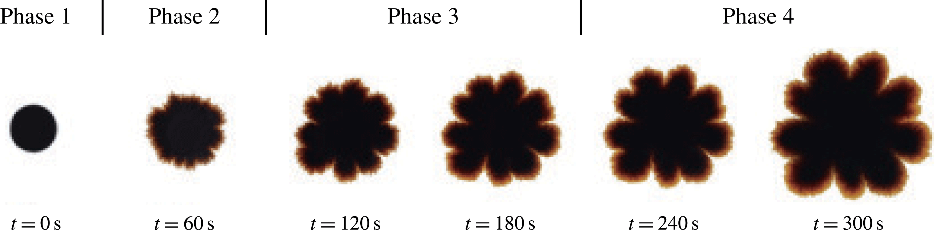
for the system to reach the maximum pre-set magnetic field strength. As time proceeds, unlike the tiny labyrinthine fingerings, secondary waves become obvious and occur with well-defined morphological distinctions. During the flow evolution, four major phases can be defined. The initial pattern as a well-defined circle is regarded as phase 1 (the original pattern). As time advances to
 $t=60~\text{s}$
(i.e. when the maximum strength has been reached), tiny fingers emerge and begin to group into several secondary waves, instead of maintaining a circular shape. The pattern with emerging labyrinthine fingering and developing secondary waves up to
 $t=60~\text{s}$
is regarded as phase 2 (the labyrinthine fingering pattern). Subsequently, the magnetic field becomes steady (
 $t>T=53.6~\text{s}$
), and the formation of secondary waves becomes more recognisable at
 $t=120~\text{s}$
but continues to develop. It is characterised by a consistent morphological pattern and an unchanged number of secondary waves in the next period, but more well-defined wave structures are observed in later periods. The flow evolution between
 $t=60~\text{s}$
and
 $t=180~\text{s}$
is considered as phase 3 (developing pattern). In phase 4, the fully developed flow pattern is observed when
 $t>180~\text{s}$
, where each secondary wave of the magnetic drop can be easily distinguished with a fine crest and valley. As time proceeds, the magnetic microconvection gradually weakens due to expansion and thus leads to a reduction in the gradient of the magnetic field along the radial direction. In contrast, a diffusion effect is much easier to identify by the smears that lead to the mixing front even though the miscible process occurs in a relatively mild way.
Growth from
 $t=0~\text{s}$
to
 $t=300~\text{s}$
(
 $0~\text{s}\geqslant t\geqslant 300~\text{s}$
) in intervals of 60 s of a magnetic drop confined in a Hele-Shaw cell with
 $h=1.0~\text{mm}$
with experimental conditions of EMG905,
 $H=300~\text{Oe}$
and
 $SR=5.6~\text{Oe}~\text{s}^{-1}$
.

Notably, regardless of the nature of the three-dimensional effect of the secondary waves, magnetisation of magnetic fluid by an external magnetic field is clearly one of the most significant factors in triggering the secondary wave and in particular magnetic-induced microconvection, as reported by Wen et al. (Reference Wen, Lin, Chen, Chen and Liang2011). They also showed that no secondary waves can be observed in the absence of an external magnetic field. In a steady case,
 $SR$
can be regarded as infinite, and finite
 $SR$
can therefore be treated as a slower process of magnetisation. Essentially, magnetic dipolar repulsion is increased by magnetisation, which can suppress the Brownian relaxation and Néel relaxation so that magnetic dipoles are consistently able to maintain their alignment with the magnetic field with fewer perturbations. In particular, the local magnetostatic potential on the diffuse interface, which is further distinguished from the state of the surrounding non-magnetic fluid, is proportional to the magnetisation (Jackson et al.
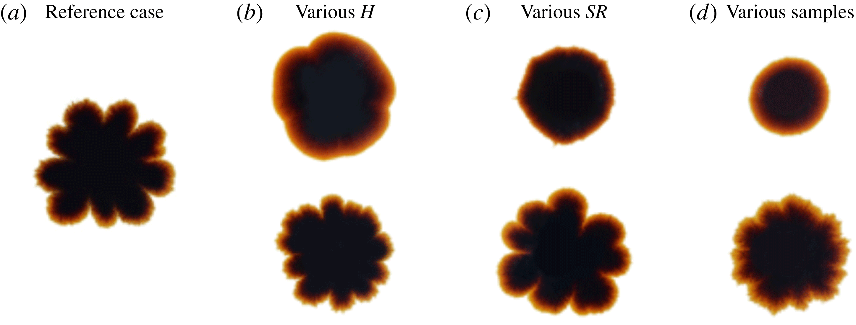
Reference Jackson, Goldstein and Cēbers1994). Therefore, factors related to the magnetisation of magnetic fluid can be regarded as the keys to the secondary waves. As shown in figure 6, the morphological state at
 $t=300~\text{s}$
from the experimental settings in figure 5 (i.e. maximum strength
 $H=300~\text{Oe}$
,
 $h=1.0~\text{mm}$
,
 $SR=5.6~\text{Oe}~\text{s}^{-1}$
, sample EMG905) is chosen as a reference for comparison with other final morphological states at
 $t=300~\text{s}$
by setting three control variables while changing only one variable.
Comparison of morphological patterns at
 $t=300~\text{s}$
: (a) reference case of the pattern at
 $t=300~\text{s}$
with experimental conditions of
 $H=300~\text{Oe}$
,
 $h=1.0~\text{mm}$
,
 $SR=5.6~\text{Oe}~\text{s}^{-1}$
, EMG905; (b) upper, EMG905,
 $SR=5.6~\text{Oe}~\text{s}^{-1}$
and
 $H=100~\text{Oe}$
; lower, EMG905,
 $SR=5.6~\text{Oe}~\text{s}^{-1}$
and
 $H=200~\text{Oe}$
; (c) upper, EMG905,
 $SR=1.4~\text{Oe}~\text{s}^{-1}$
and
 $H=300~\text{Oe}$
; lower, EMG905,
 $SR=2.8~\text{Oe}~\text{s}^{-1}$
and
 $H=300~\text{Oe}$
; (d) upper, EMG911,
 $SR=5.6~\text{Oe}~\text{s}^{-1}$
and
 $H=300~\text{Oe}$
; lower, EMG909,
 $SR=5.6~\text{Oe}~\text{s}^{-1}$
and
 $H=300~\text{Oe}$
.

The effect of the pre-set maximum magnetic field can be analysed from figure 6(a,b), in which magnetic drops are subjected to different magnetic fields with the same
 $SR=5.6~\text{Oe}~\text{s}^{-1}$
. The magnetic drops expand as expected and evolve into two distinguishable morphological states. After reaching its maximal magnetic field for a certain period, the observations are similar to those for the steady cases (Wen et al.
Reference Wen, Lin, Chen, Chen and Liang2011). However, unlike the system of infinite sweep rate of the magnetic field, the magnetic drop is exposed to a low magnetic field during the early period, when diffusion is the major factor to facilitate the growth of the magnetic field while it is also growing. For the lowest pre-set maximum magnetic field strength, i.e.
 $H=100~\text{Oe}$
, it is difficult to identify whether well-defined secondary waves have been formed, but there are approximately four obscure secondary wave structures. Diffusion plays a significant role, while the perturbations from magnetic repulsions here are therefore less significant than those that merely come with obscure floccules within the smears. As a result, the expansion growth is dominated by diffusion in which the mixing process on the interface contributes an obvious component to the pattern of the magnetic drop when the magnetic effect is weakened. In addition, smears on this large scale can result from the contact counterflows that arise in the lower and upper parts of a Hele-Shaw cell due to gravity (Ērglis et al.
Reference Ērglis, Tatulcenkov, Kitenbergs, Petrichenko, Ergin, Watz and Cēbers2013), which smear out the concentration distribution and hence smear a wider transition layer. Nevertheless, good formation of well-defined secondary waves can be clearly observed with nearly
 $n\simeq 10$
as the pre-set value for a maximum magnetic field strength of
 $H=200~\text{Oe}$
. Under the action of a ponderomotive force due to non-collinearity between the concentration gradient and the magnetic field gradient, magnetic microconvection is triggered, and the magnetic fingerings extend into the miscible non-magnetic fluid (Ērglis et al.
Reference Ērglis, Tatulcenkov, Kitenbergs, Petrichenko, Ergin, Watz and Cēbers2013; Kitenbergs et al.
Reference Kitenbergs, Tatulcenkovs, Ērglis, Petrichenko, Perzynski and Cēbers2015). Therefore, the magnetic microconvection of magnetic fluid subjected to a greater magnetic field is accelerated and further enhanced, particularly on the interface. In this case, smears are not as significant as in the previous case along with branches of sub-waves on a secondary wave. Secondary wave structures are strengthened with a greater magnetic field strength of
 $H=300~\text{Oe}$
, while smears are imaged in a much less significant way.
By reaching the same amplitude of the magnetic field, different values of
 $SR$
chronically affect different levels of magnetisation. Comparing figures 6(a) and 6(c), an irregular pattern subjected to
 $SR=1.4~\text{Oe}~\text{s}^{-1}$
occurs without secondary waves but with a relatively sharp boundary; a circular shape is also not formed. Once the experiment begins, a magnetic field with a low
 $SR$
slowly magnetises the magnetic fluid, and, meanwhile, the magnetic drop begins to expand due to diffusion. However, diffusion consistently dominates the growth process when the magnetisation is not strong enough and the radius of the magnetic drop continues to grow. Therefore, even when the magnetic field reaches its maximum, the enlarged area of magnetic fluid has greatly reduced the concentration of magnetic nanoparticles, especially the lower gradient of concentration on the diffused interface, which slows growth. Consequently, the distance between each pair of magnetic dipoles is elongated, and the repulsion due to their interaction is therefore diminished during the growth of the magnetic drop, so that perturbations that result from magnetic dipolar repulsion become quite insignificant even though the magnetic field reaches its maximum after approximately 214 s, as listed in table 1. By setting faster values of the
 $SR$
of the magnetic field, as in the lower part of figure 6(c) (
 $SR=2.8~\text{Oe}~\text{s}^{-1}$
) and figure 6(a) (
 $SR=5.6~\text{Oe}~\text{s}^{-1}$
), secondary waves are successfully triggered, and well-defined wave structures can be observed with various secondary waves. In these cases, by doubling the
 $SR$
, the magnetisation proceeds more quickly and ensures that the occurrences of magnetic repulsion are significant before the distance increases too much to provide strong enough perturbations from magnetic dipolar repulsion. Another interesting feature is that the smear on the leading interface in the case of figure 6(c) is not as wide as that in the upper case of figure 6(b) even with a higher
 $SR$
of
 $5.6~\text{Oe}~\text{s}^{-1}$
. The other variable that differs between them is the maximum magnetic field strength, which is
 $H=100~\text{Oe}$
for figure 6(b) but
 $H=300~\text{Oe}$
for figure 6(c). The magnetic field should have a faster
 $SR$
and should be strong enough to trigger secondary waves. During the whole process, based on the analysis above, the simple hypothesis can be made that the time scale of the magnetic effect increases dynamically with the growth distance, but is shortened by a larger maximum magnetic field and faster
 $SR$
, where a Péclet number will be described later, compared with the diffusion.
Another comparison among different samples is also observed, as shown in figure 6(a,d). Various samples have different saturation magnetisations which originate from their corresponding particle concentrations, as shown in table 2. An extremely round morphological pattern is formed along with a wide smear by the magnetic drop of sample EMG911, the magnetic effect of which is quite weak even under many other sets of experimental conditions and is dominated by diffusion. It should be noted that the particle concentration and saturation magnetisation of EMG911 are the lowest of the three samples, so strong enough perturbation by magnetic dipolar repulsions may be quite difficult to reach compared with the other two samples with two or even four times the saturation magnetisation. Secondary waves do come into observation for samples of EMG909 and EMG905. In the lower case of figure 6(d) (EMG909 at
 $t=300~\text{s}$
), the prominence of the secondary waves is similar to that in phase 2 of EMG905 at
 $t=60~\text{s}$
in figure 5, the defined structure of secondary waves of which is less smooth than the well-developed ones in figure 6(a). In this perspective, the case of EMG911 discussed above is similar to phase 1 of EMG905 at
 $t=0~\text{s}$
in figure 5. From our observations for
 $t>300~\text{s}$
, both cases in figure 6(d) retain their patterns, and no further fine secondary waves structures develop. This might have interesting implications. If the magnetic fluid EMG905 under the current experimental setting can represent a fully secondary wave development track in figure 5, then the other two magnetic fluids, EMG909 and EMG911, with lower particle concentrations and hence lower magnetisation ability, can only evolve to the early phases of EMG905, the secondary wave structure of which is not fully developed and possibly cannot be developed.
4 Quantitative analysis
4.1 Quantification
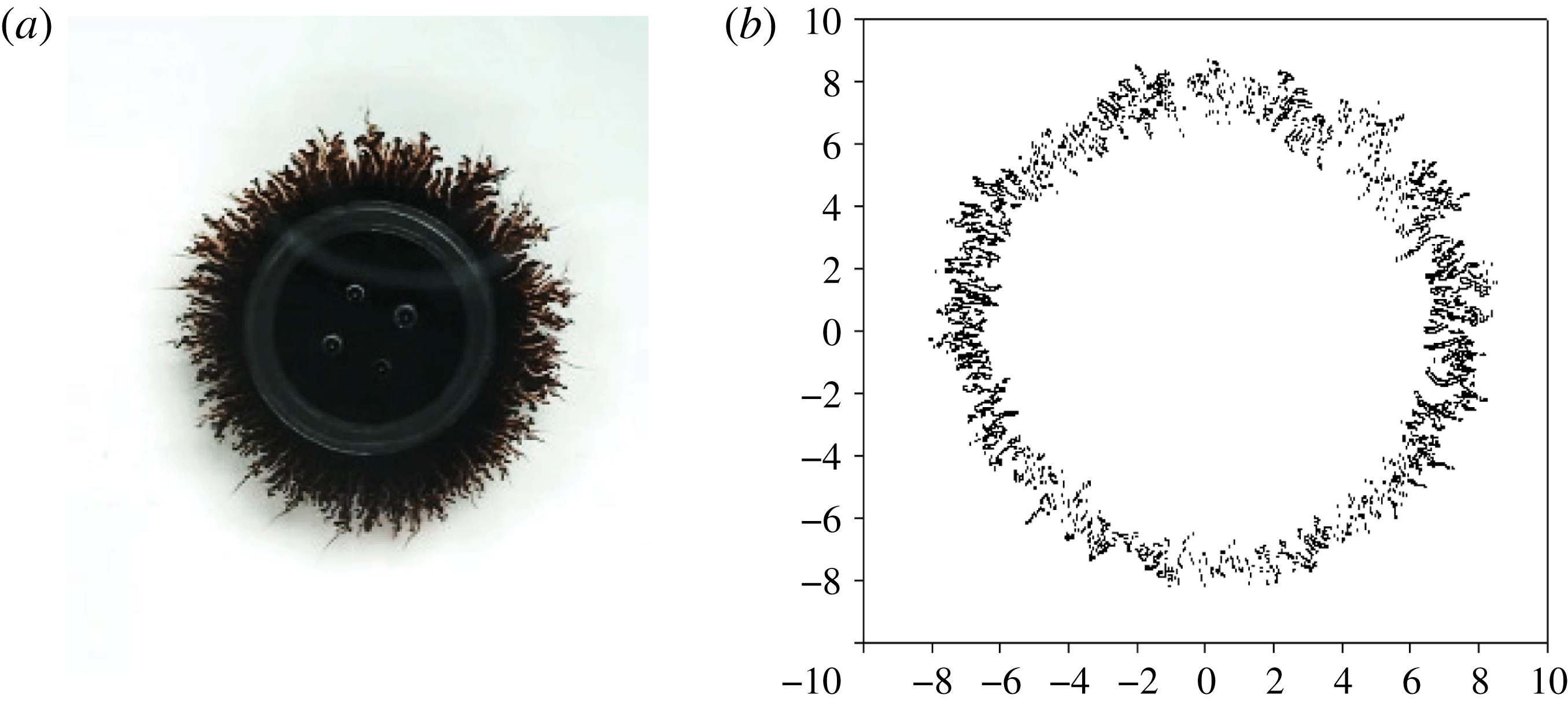
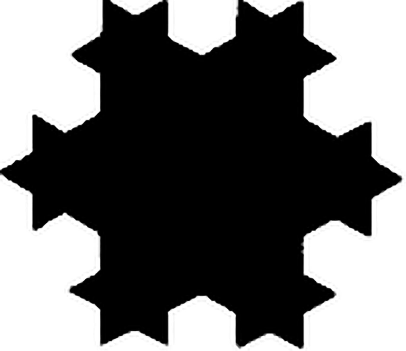
To quantify the morphological pattern, the captured colour image file from the camera was transferred into an 8-bit greyscale bitmap file (with a grey level value of 255 as pure white) with a Matlab program, as shown in figure 7. Figure 7(a) is the image taken by the Nikon D7000 camera and figure 7(b) is the interface recognised by the Matlab program from image figure 7(a). The interfacial boundary is defined at a grey value of 240. The interfacial length
 $L$
is then calculated by adding the distance between each pair of neighbouring points on the interface based on the recognition in figure 7(b). A regular pattern with 48 3.32 mm long segments and a total length of 159.36 mm (figure 8) is used to calibrate the accuracy of the Matlab program. Our calculation by Matlab is 161.60 mm, with an error of
 $1.4\,\%$
, which is considered to be acceptable in this study. The interfacial length (
 $L$
) is scaled by the original interfacial length,
 $L_{0}=2\unicode[STIX]{x03C0}R_{0}$
, where
 $R_{0}$
is the initial radius of the magnetic drop, 7.5 mm, and hence defines a dimensionless interfacial length,
 $L^{\ast }=L/L_{0}$
. The time
 $t$
is scaled by the diffusion time scale,
 $t_{d}=h^{2}/D$
, where
 $D$
is the diffusivity, calculating the dimensionless time,
 $t^{\ast }=t/t_{d}$
, and the relationship between
 $L^{\ast }$
and
 $t^{\ast }$
for typical cases is introduced for quantitative analysis in a later section.
Quantification of interfacial length: (a) the magnetic drop image taken by the charge-coupled device (CCD); (b) interfacial recognition by Matlab.

Regular pattern for interfacial length calibration, which consists 48 3.32 mm long segments with a total length of 159.36 mm. The interfacial length is calculated as 161.60 mm by our Matlab program.

The method to determine the number of secondary waves,
 $n$
, is also introduced here. As reported by Wen et al. (Reference Wen, Lin, Chen, Chen and Liang2011), labyrinthine instabilities and the prominent secondary waves of magnetic fluids can be regarded as small perturbations of magnetic dipolar repulsion, and the number of secondary waves,
 $n$
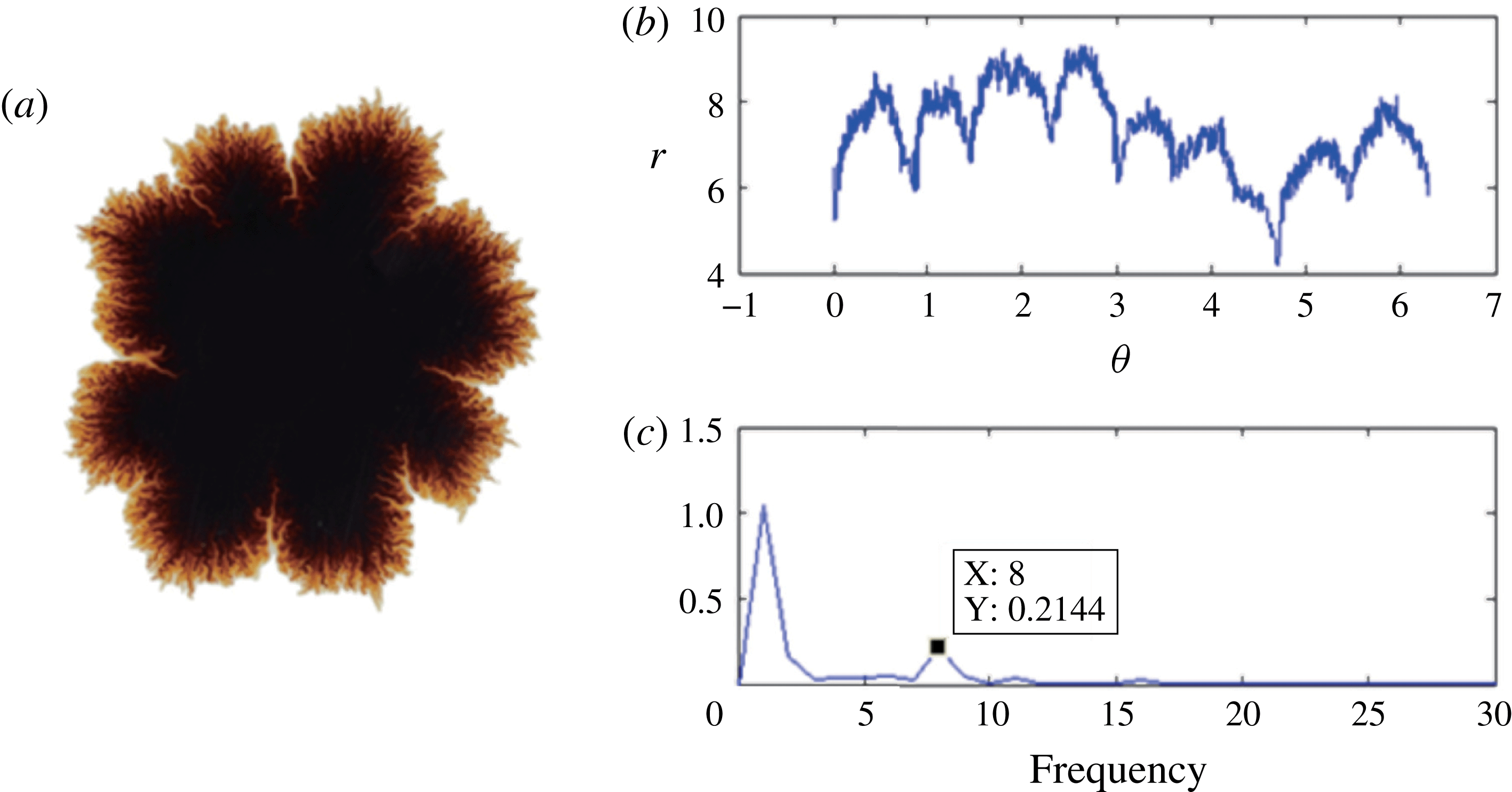
, can be analysed by fast Fourier transform. An example is demonstrated in figure 9. A polar representation of the interface of figure 9(a), the relationship between the radius
 $r$
and the corresponding angular position, is shown in figure 9(b). The polar representation is further analysed by fast Fourier transform, as shown in figure 9(c), with Matlab. The first peak in figure 9(c) denotes the circle interface, and the second is for the secondary waves.
(a) Morphological image; polar representation analysed by (b) Matlab and (c) fast Fourier transform.

4.2 Early interfacial growth
The interfacial length of the magnetic drop is used for characterisation of the growth of instabilities in the early period (i.e.
 $t\leqslant 20~\text{s}$
). Four major factors that affect the early growth of instabilities are introduced, including the sweep rate (
 $SR$
), the maximum magnetic field (
 $H$
), samples and gap spans (
 $h$
). A typical growth curve for the interfacial length is shown in figure 10, for which the magnetic fluid EMG905 was used (
 $SR=2.8~\text{Oe}~\text{s}^{-1}$
,
 $H=100~\text{Oe}$
and
 $h=1.0~\text{mm}$
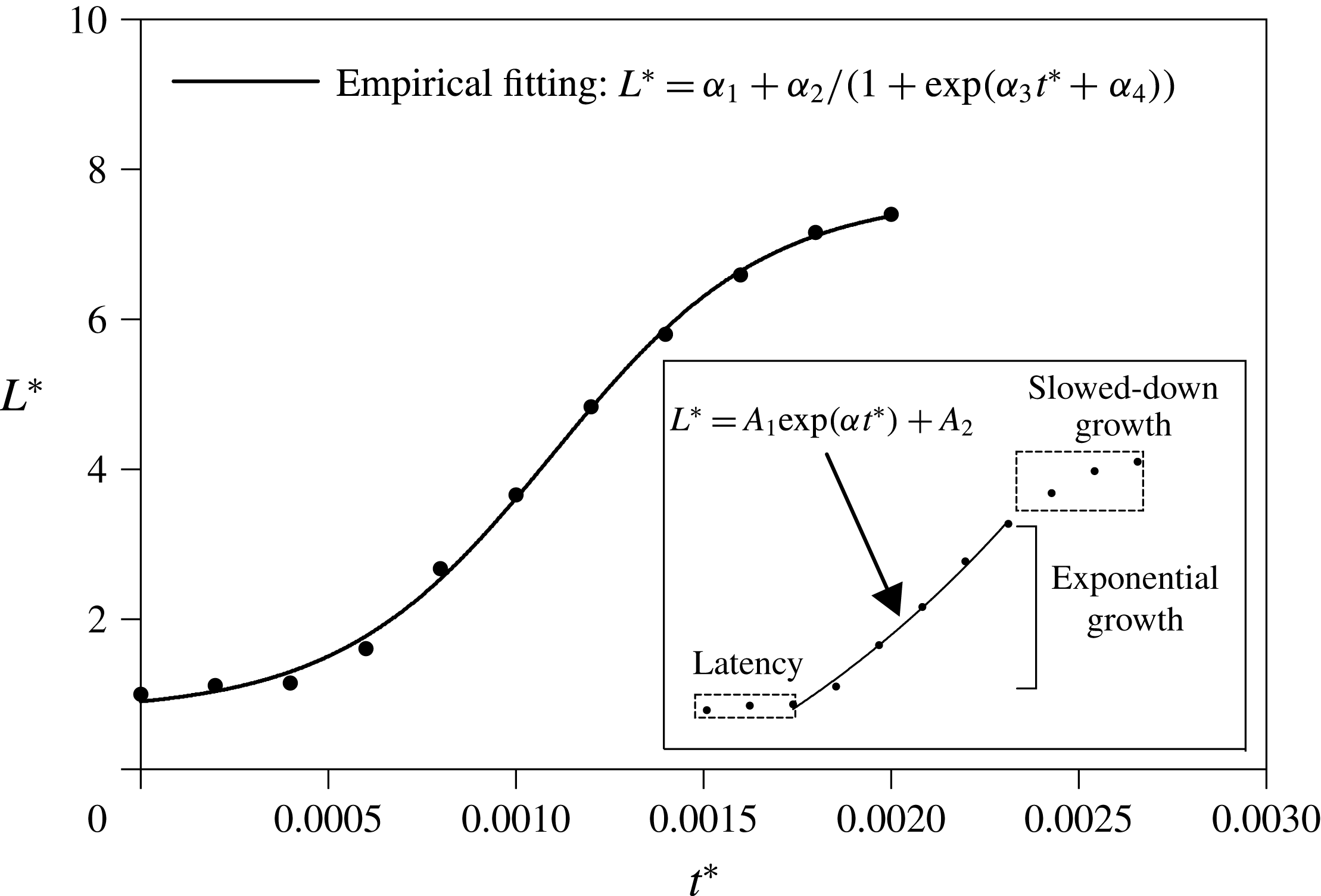
). Instead of merely using scattering points on the curves, a logistic function,
 $L^{\ast }=\unicode[STIX]{x1D6FC}_{1}+\unicode[STIX]{x1D6FC}_{2}/(1+\exp (\unicode[STIX]{x1D6FC}_{3}t^{\ast }+\unicode[STIX]{x1D6FC}_{4}))$
, is used to fit the curves for a better description of the growth trends. This model includes the three significant features: latency, exponential growth and slowed-down growth. Generally, at the very beginning of the experiments, the magnetic field just begins; meanwhile, diffusion just sets in. Magnetic microconvection is hardly induced. In this regard, inertia and static friction may play a role in preventing motion of the magnetic fluid. Therefore, the interfacial length grows in a rather slow way, which can be clearly identified as the initial latency period. After the latency period, as the strength of the magnetic field rises, magnetisation of the magnetic fluids, and hence the action of magnetic repulsions from magnetic dipoles, is reinforced. Consequently, labyrinthine instabilities emerge in the form of numerous tiny fingerings that extend into the miscible surroundings (diesel), as shown in figure 4. Therefore, the interfacial length increases in an exponential manner by adding the doubled radial lengths of these emerging tiny fingerings to characterise the exponential growth in the growth curve. Notably, after the exponential growth, the slope of the growth curve begins to level off and later decreases due to the smear of the interface caused by diffusion. This period is denoted as slowed-down growth, as shown in figure 10. In particular, exponential growth can be clearly distinguished from the two other periods (i.e. latency and slowed-down growth), as shown in the inset of figure 10, due to its dramatically increasing trend.
The mathematical model to fit the growth curves, which can include the latency, the exponential growth and the slowed-down growth periods. Inset: initial growth rate (
 $\unicode[STIX]{x1D6FC}$
) definition, in which the exponential growth section is extracted for exponential fitting by the equation
 $L^{\ast }=A_{1}\exp (\unicode[STIX]{x1D6FC}t^{\ast })+A_{2}$
. Experimental conditions: EMG905,
 $SR=2.8~\text{Oe}~\text{s}^{-1}$
,
 $H=100~\text{Oe}$
,
 $h=1.0~\text{mm}$
.

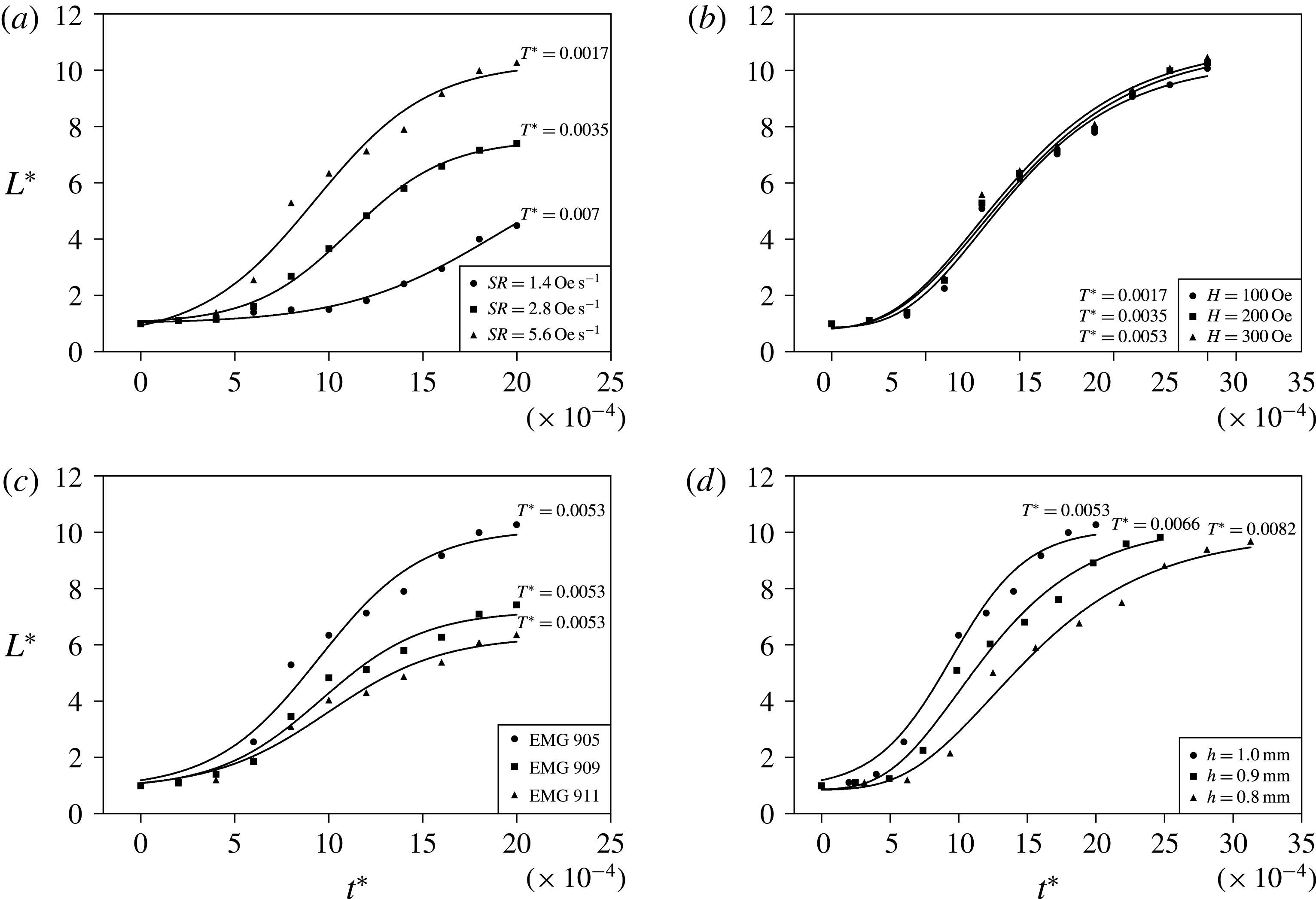
Growth of the interfacial length under different sets of experimental conditions, where the corresponding
 $T^{\ast }$
is shown: (a) EMG905,
 $h=1.0~\text{mm}$
,
 $H=100~\text{Oe}$
; (b) EMG905,
 $SR=5.6~\text{Oe}~\text{s}^{-1}$
,
 $h=1.00~\text{mm}$
; (c)
 $h=1.00~\text{mm}$
,
 $SR=5.6~\text{Oe}~\text{s}^{-1}$
,
 $H=300~\text{Oe}$
; (d) EMG905,
 $H=300~\text{Oe}$
,
 $SR=5.6~\text{Oe}~\text{s}^{-1}$
. A logistic function
 $L^{\ast }=\unicode[STIX]{x1D6FC}_{1}+\unicode[STIX]{x1D6FC}_{2}/(1+\exp (\unicode[STIX]{x1D6FC}_{3}t^{\ast }+\unicode[STIX]{x1D6FC}_{4}))$
is used to fit for the whole early growth trend observation.

In figure 11, growth curves for different experimental conditions are illustrated. The importance of
 $SR$
is shown in figure 11(a) with dimensionless sweeping times
 $t^{\ast }$
. Growth curves with different values of
 $SR$
show clear distinctions. It is noteworthy that, during the observation period (
 $t\leqslant 20~\text{s}$
or
 $t^{\ast }\leqslant 0.0025$
), the magnetic field does not reach its maximum but continues to increase; that is,
 $t^{\ast }\leqslant T^{\ast }$
(the dimensionless sweep time
 $T^{\ast }$
). The latency for higher values of
 $SR$
is shortened by the faster rise of the magnetic field, characterising that perturbations from magnetic dipolar repulsions can be triggered and facilitated in a more intensive way by enlarging the
 $SR$
to push the growth from an earlier moment. Following the mild latency period, a dramatic variety occurs in the branches of exponential growth for different values of
 $SR$
. A higher
 $SR$
contributes to steeper growth for the interfacial length and larger slopes of the growth curves for
 $SR=2.8~\text{Oe}~\text{s}^{-1}$
and
 $SR=5.6~\text{Oe}~\text{s}^{-1}$
after latency. For the lowest
 $SR=1.4~\text{Oe}~\text{s}^{-1}$
, the growth of the interfacial length is considerably slower than in the other two cases due to the small magnetic advection and relatively long diffusion time. The slope of the growth curve for
 $SR=1.4~\text{Oe}~\text{s}^{-1}$
consistently increases over time, and reduction has not yet been observed because of the growing magnetic field (
 $t^{\ast }\leqslant T^{\ast }=0.007$
), indicating that low
 $SR$
elongates the period for the tiny fingerings to grow or stabilise. As previously mentioned, the initial growth rate of interest is unstable and the investigated period is before the magnetic field reaches its maximum. If one then follows the interface growth until
 $t=300~\text{s}$
, secondary waves will not be found, similarly to the upper image of figure 6(b). In addition, a slower
 $SR$
delays the occurrence of labyrinthine instabilities, as shown in figure 4(a), from 4 s for
 $SR=5.6~\text{Oe}~\text{s}^{-1}$
to 14 s for
 $SR=1.4~\text{Oe}~\text{s}^{-1}$
. A slow
 $SR$
hinders the prominence of the secondary wave, and by suppressing the
 $SR$
the possibility for secondary waves is eventually lost because the diffusion has weakened the magnetic effect on the interface by enlarging the radius. If
 $SR$
is set as infinitesimal or zero, the growth of instabilities is purely concluded into the diffusion regime without a magnetic field and thus a secondary wave, because magnetic microconvection must be absent from the growth of instabilities. In addition, the case of
 $SR=5.6~\text{Oe}~\text{s}^{-1}$
still obtains the highest interfacial length in the later period by reaching its maximum at
 $t^{\ast }=T^{\ast }=0.0017$
. Therefore, the phenomenon of a greater exponential growth for interfacial length should be mainly due to a faster
 $SR$
.
Figure 11(b) illustrates three highly overlapping growth curves of magnetic fields with the same
 $SR=5.6~\text{Oe}~\text{s}^{-1}$
and different pre-set maxima for the magnetic field. In this study, the fastest sweeping time is
 $T^{\ast }=0.0017$
, as mentioned above, so magnetic fields
 $t^{\ast }<T^{\ast }=0.002$
with the same
 $SR$
are essentially the same. Therefore, by merely changing the pre-set maximum of the magnetic field strength within a specific range, differentiation among them is less likely to be observed during the early period. Their importance, however, occurs in the later period because the magnetic fields stabilise and reach their corresponding maxima. The magnetism-induced microconvection under a higher magnetic field is stronger due to the enhanced magnetic dipolar repulsions, which can be verified and characterised by the intensity of the secondary waves in figure 6(a,d).
Investigations of different magnetic fluids are also illustrated in figure 11(c), and their durations of latency and dimensionless sweeping time
 $T^{\ast }$
are nearly the same. At the very beginning, the magnetic field strength is close to zero, and the magnetic drop diffuses outward subjected to the same external force, such as viscous force. Nevertheless, the three magnetic fluids become different at the termination of latency because the magnetisation of the magnetic drop becomes significant. The sample of EMG905 contains more magnetic nanoparticles due to its higher concentration, and therefore more magnetic moments are able to contribute to the magnetisation microscopically compared with the other samples with lower concentrations. Magnetic dipolar repulsions occur and push the magnetic drop outward in a stronger manner than in the other two samples. As time proceeds, exponential increases occur as expected for characterisation of the intensive labyrinthine instabilities due to the same
 $SR$
. However, the magnetic fluid EMG911 under this set of experimental conditions (
 $h=1.00~\text{mm}$
,
 $SR=5.6~\text{Oe}~\text{s}^{-1}$
and
 $H=300~\text{Oe}$
) fails to evolve secondary waves in the later period (
 $t=300~\text{s}$
), as shown in the upper part of figure 6(c). This finding implies that the concentration of the magnetic fluid is also a factor that affects the prominence of secondary waves, as analysed in the previous section; the mechanism will be discussed in a later section.
Differences in gap span settings also play an important role in the growth of instabilities in the early period, as shown in figure 11(d), with the same magnetic field, sweep rate and magnetic fluid, where the growth curves of the three different samples are quite different. Similarly to the way that
 $SR$
affects the growth of instabilities, among these curves in figure 11(d), the duration of latency can be clearly distinguished by altering the gap span and the subsequent exponential growth. After the latency, the interfacial length for larger gaps gains a steeper growth trend. The elongation of the latency can be attributed to the change, by varying the gap, of the time scale,
 $t_{d}=h^{2}/D$
, where a larger gap span leads to a smaller dimensionless time. The viscous force is induced by the friction between the wall and the fluids, following an equation based on Darcy’s Law. Therefore, the viscous force increased by a smaller gap span also slows the growth of the interfacial length and hence leads to a longer period of latency and slower growth.
The initial growth rate,
 $\unicode[STIX]{x1D6FC}$
, is defined according to the linear stability analyses of Igonin & Cēbers (Reference Igonin and Cēbers2003), Ērglis et al. (Reference Ērglis, Tatulcenkov, Kitenbergs, Petrichenko, Ergin, Watz and Cēbers2013) and Kitenbergs et al. (Reference Kitenbergs, Tatulcenkovs, Ērglis, Petrichenko, Perzynski and Cēbers2015) for the magnetic fluid instability, in which the fingering velocity follows the exponential growth. Hence, an exponential equation,
 $L^{\ast }=A_{1}\exp (\unicode[STIX]{x1D6FC}t^{\ast })+A_{2}$
, was used to fit the exponential growth part of the non-dimensional interfacial length, as shown in figure 10. Standard deviations of the fitting regression are used to define the error bars of
 $\unicode[STIX]{x1D6FC}$
. The initial growth inherently represents the fastest-growing mode of the magnetic drop in the Hele-Shaw cell. Following the reported work of Wen et al. (Reference Wen, Lin, Chen, Chen and Liang2011), the initial growth rates of the interfacial lengths
 $\unicode[STIX]{x1D6FC}$
for 81 sets of experimental conditions, including different samples, gap spans (
 $h$
), sweep rates (
 $SR$
) and maximum magnetic field (
 $H$
), can be correlated with a modified Péclect number,
 $Pe^{\prime }$
. The modified Péclect number
 $Pe^{\prime }$
is defined in (4.1) as the ratio of the diffusion time scale
 $t_{d}$
and the magnetic advective time scale
 $t_{m}$
(more detailed derivations are given in appendix A), and
 $\text{d}M/\text{d}t$
is approximately expressed as due to the different maximum stable magnetic field, where
 $D$
represents the diffusivity,
 $\unicode[STIX]{x1D707}_{0}$
represents the permeability in free space and
 $\unicode[STIX]{x1D712}_{0}$
represents the effective susceptibility,
 $$\begin{eqnarray}Pe^{\prime }=\frac{t_{d}}{t_{m}}=\frac{h^{2}/D}{[12h^{2}\unicode[STIX]{x1D70C}\unicode[STIX]{x1D712}_{0}/\unicode[STIX]{x1D707}_{0}(\text{d}M/\text{d}t)^{2}]^{1/4}}.\end{eqnarray}$$
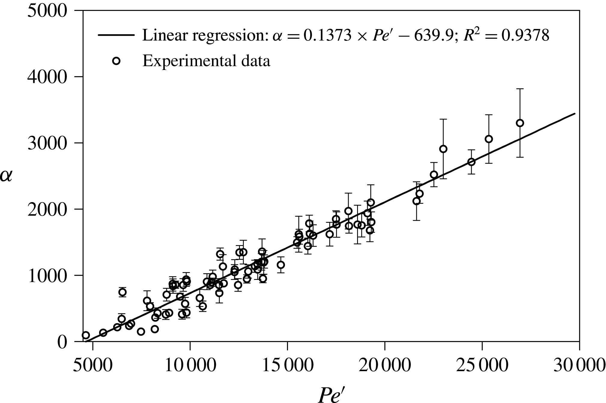
Linear regression correlates the initial growth rate and the modified Péclect number
 $Pe^{\prime }$
, as shown in figure 12. The initial growth rate increases linearly and monotonically with
 $Pe^{\prime }$
following the equation
 $\unicode[STIX]{x1D6FC}=0.1373Pe^{\prime }-639.9$
, with
 $R^{2}=0.9378$
. A good collapse in a linear relation has been obtained. Intuitively,
 $L\sim R$
at the early stage of interface evolution and
 $t\sim t_{m}$
(the magnetic advection time scale) in the exponential growth period. Therefore, according to the definition of the initial growth rate,
 $\unicode[STIX]{x1D6FC}\equiv (\text{d}L^{\ast }/\text{d}t^{\ast })_{t^{\ast }\rightarrow 0}\sim (L/2\unicode[STIX]{x03C0}R)/(t/t_{d})\sim (R/2\unicode[STIX]{x03C0}R)/(t_{m}/t_{d})=(1/2\unicode[STIX]{x03C0})Pe^{\prime }\sim 0.159Pe^{\prime }$
. The estimated slope of 0.159 is very close to the experimental correlation value of 0.1373. Moreover, in the linear regression results of Kitenbergs et al. (Reference Kitenbergs, Tatulcenkovs, Ērglis, Petrichenko, Perzynski and Cēbers2015), a relationship was found between the maximum velocity of the instability fingers and the magnetic Rayleigh number, and the maximum velocity was experimentally and numerically measured and found to increase linearly with the magnetic Rayleigh number, with slopes of
 $0.27\pm 0.03$
and
 $0.36\pm 0.01$
respectively. This trend is quite similar to the current results, with slopes of around 0.1373, even though there are a few differences in the formulation between the current Péclect number and the magnetic Rayleigh number
 $Ra_{m}$
defined by Kitenbergs et al. (Reference Kitenbergs, Tatulcenkovs, Ērglis, Petrichenko, Perzynski and Cēbers2015). The physical meanings for both dimensionless numbers are essentially the same and are calculated by the ratio between the diffusion time scale and the magnetic time scale, while their definition is based on a steady magnetic effect. As mentioned above, the initial growth rate is the increase in the interfacial length, so that it contains most of the changes that occur on the interface, especially the length of the labyrinthine fingerings, instead of merely focusing on the fastest one. This may be one reason that explains the difference. Another point is that this is an unsteady case in our study, and magnetic microconvection is being accelerated while the magnetic field is still growing. However, the growth of the magnetic field in the study of Kitenbergs et al. (Reference Kitenbergs, Tatulcenkovs, Ērglis, Petrichenko, Perzynski and Cēbers2015) is fulfilled because of their steady magnetic field (
 $SR\rightarrow \infty$
). Therefore, the intensities of microconvection between these two studies are not completely the same, but the similar results should lead us to notice the subtle common mechanism behind them. Notably, the diffusion coefficient between the magnetic fluid and the base fluid, diesel, has been poorly studied so far. In this experimental analysis, the diffusion coefficient of
 $10^{-10}~\text{m}^{2}~\text{s}^{-1}$
provided by Ferrotec Corp. (Tokyo, Japan) was used to calculate
 $Pe^{\prime }$
. To further analyse the physical meaning of (4.1), it can be further expressed as follows:
 $$\begin{eqnarray}Pe^{\prime }\propto h^{3/2}\left(\frac{\unicode[STIX]{x1D712}_{H}^{2}}{\unicode[STIX]{x1D70C}\unicode[STIX]{x1D712}_{0}}\right)^{1/4}SR^{1/2}.\end{eqnarray}$$
The modified Péclect number
 $Pe^{\prime }$
is then proportional to three major factors, namely the gap factor,
 $h^{3/2}$
, for the three-dimensional effect of the Hele-Shaw cell, the material factor,
 $(\unicode[STIX]{x1D712}_{H}^{2}/\unicode[STIX]{x1D70C}\unicode[STIX]{x1D712}_{0})^{1/4}$
, for the nature of the tested sample and the magnetic factor,
 $SR^{1/2}$
, for the effect due to the sweep rate. The facilitation by enlarging the gap span (
 $h$
) and the sweep rate (
 $SR$
) indicated by this equation is consistent with the experimental results, as shown in figure 11. Moreover, the choices for samples are also verified by the growth curves above, for the enhancement of the growth, whose values of
 $(\unicode[STIX]{x1D712}_{H}^{2}/\unicode[STIX]{x1D70C}\unicode[STIX]{x1D712}_{0})^{1/4}$
are largest for EMG905, followed by those for EMG909 and EMG911 for the same magnetic field. Therefore, by choosing a magnetic fluid with a higher ratio between susceptibility and density,
 $Pe^{\prime }$
can be increased and therefore predicts the linear increase in the growth rate. Information from the definition of
 $Pe^{\prime }$
also implies that the initial growth is irrelevant to the maximum pre-set value of the magnetic field, which can be clearly observed in figure 11(b). In summary, each of these three factors can physically shorten the time scale or accelerate the advection rate due to a magnetic effect and can further give a precise characterisation of the contributions from each component, which shows strong consistency with the experimental observations. Notably, due to the poor temporal resolution of the interfacial length, the growth rate was overestimated by Wen et al. (Reference Wen, Lin, Chen, Chen and Liang2011).
Linear regression for the initial growth rate and the modified Péclect number
 $Pe^{\prime }$
from 81 points representing 81 sets of experimental conditions.

4.3 Magnetic regime of secondary waves
Based on the results analysed in the previous section, the dependence of the growth rate on the modified Péclect number
 $Pe^{\prime }$
has been validated again in a large parameter space with various sets of experimental conditions during the early period (
 $t\leqslant 20~\text{ s}$
). Development of the labyrinthine instabilities from the early period further continues as time proceeds, and they evolve into a state of well-defined secondary waves. The gap effect is further analysed due to the verified relationship between secondary waves and the three-dimensional effect (Wen et al.
Reference Wen, Chen and Kuan2007a
). As mentioned above, the prominence of secondary waves is induced by magnetic microconvection, and the strong dependence on the modified Péclect number
 $Pe^{\prime }$
during the early period shows that magnetic convection can be reinforced by increasing
 $Pe^{\prime }$
. Associated with the most outstanding feature of secondary waves, the countable number of secondary waves,
 $n$
, can be obtained by visualisation analysis at
 $t=300~\text{s}$
with a Matlab program, as mentioned above. The wavelengths of the secondary waves of the magnetic drop were calculated for each set of experimental conditions by the definition
 $\unicode[STIX]{x1D706}=2\unicode[STIX]{x03C0}R_{0}/n$
, as reported in our previous work (Wen et al.
Reference Wen, Chen and Kuan2007a
). Furthermore, the dependence of the wavelengths on the gap span was also investigated (Wen et al.
Reference Wen, Chen and Kuan2007a
). The wavelength,
 $\unicode[STIX]{x1D706}$
, is first non-dimensionalised by the gap width,
 $h$
, and the dimensionless wavelength,
 $\unicode[STIX]{x1D6EC}=\unicode[STIX]{x1D706}/h$
, is then correlated with
 $Pe^{\prime }$
to determine how the magnetic microconvection affects the prominence of the secondary waves.
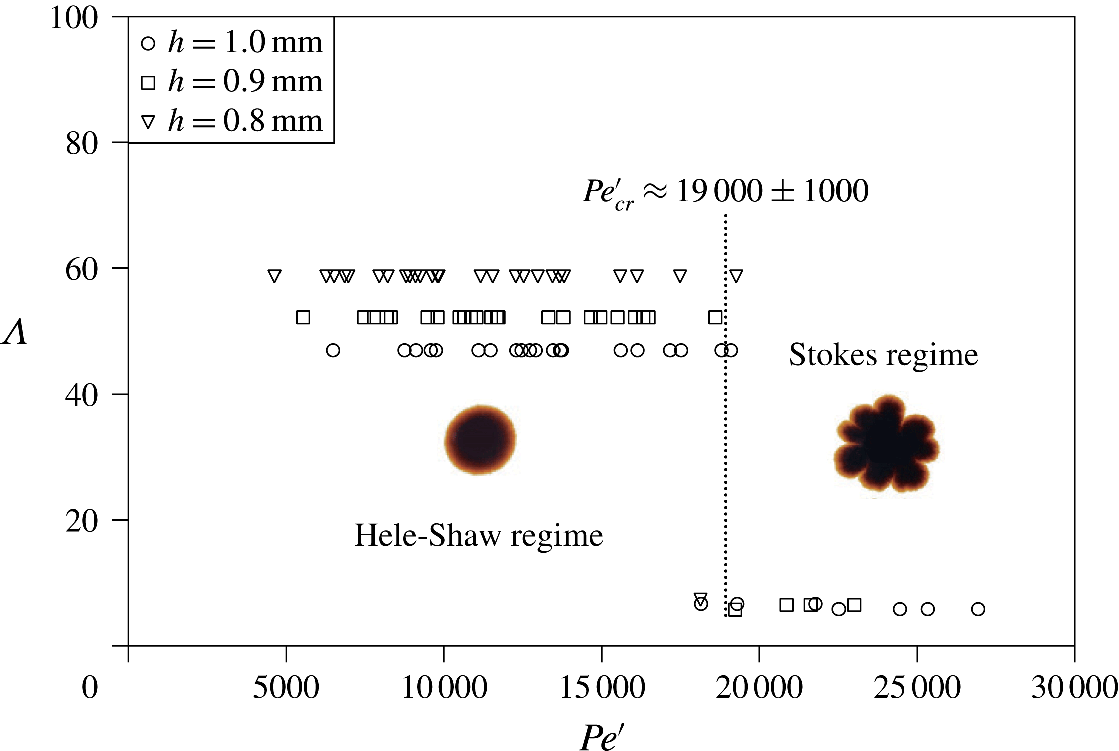
The evolution of the dimensionless wavelength
 $\unicode[STIX]{x1D6EC}$
with
 $Pe^{\prime }$
; the critical value of
 $Pe_{cr}^{\prime }$
is marked. It should be noted that the dimensionless wavelength,
 $\unicode[STIX]{x1D6EC}=\unicode[STIX]{x1D706}/h$
, is defined as the ratio of the wavelength
 $\unicode[STIX]{x1D706}$
of the largest perturbation to the circle to the gap span
 $h$
of the Hele-Shaw cell.

As shown in figure 13, a series of values for the dimensionless wavelength
 $\unicode[STIX]{x1D6EC}$
are calculated using 81 sets of experimental data to correlate with their corresponding
 $Pe^{\prime }$
values. An identical transition at around a critical
 $Pe_{cr}^{\prime }$
of 19 000 is attractive to divide the system into two regimes. Following similar definitions reported by Fernandez et al. (Reference Fernandez, Kurowski, Petitjeans and Meiburg2002), the first regime is the Hele-Shaw regime, when
 $Pe^{\prime }\leqslant 19\,000$
, and the second regime is the Stokes regime, when
 $Pe^{\prime }\geqslant 19\,000$
. The Hele-Shaw regime is characterised and governed by a two-dimensional effect. The high values of
 $\unicode[STIX]{x1D6EC}$
are due to the absence of secondary waves, and the number
 $n$
is regarded as 1. The dimensionless wavelength is reduced accordingly to
 $\unicode[STIX]{x1D6EC}=\unicode[STIX]{x1D706}/h=2\unicode[STIX]{x03C0}R_{0}/nh$
, where
 $n=1$
and
 $R_{0}$
is the initial radius of the magnetic drop, 7.5 mm, and becomes gap-dependent. Nevertheless, the experimental observations are essentially the same, featuring a circle as in the upper parts of figure 6(c–d). In contrast, the Stokes regime is governed by the three-dimensional effect. In this regime, the dimensionless wavelengths of the different gap spans,
 $\unicode[STIX]{x1D6EC}$
, collapse into a similar value,
 $m$
, at around
 $7\pm 1$
, which is the same result as concluded from our previous study (Wen et al.
Reference Wen, Chen and Kuan2007a
). The magnetic microconvection is strong enough to trigger the prominence of secondary waves, and the number of secondary waves
 $n$
is no longer equal to 1 up to a certain value and coincidently leads to an approximately constant product
 $mh$
. The value of
 $m$
is essentially independent of
 $Pe^{\prime }$
once the significance of magnetic microconvection exceeds the critical
 $Pe_{cr}^{\prime }$
value of 19 000. The stepwise transition instead of an asymptotic one near the critical value may imply the existence of a barrier. It turns out that the magnetic advection should be strong enough to trigger the secondary waves due to the definition of
 $Pe^{\prime }$
, which is quite different from the density-driven instabilities in a Hele-Shaw cell (Fernandez et al.
Reference Fernandez, Kurowski, Petitjeans and Meiburg2002). After coupling the complexity of the mechanism for secondary wave formation into
 $Pe^{\prime }$
, which includes four major factors – maximum magnetic field (
 $H$
), sweep rate (
 $SR$
), samples and gap (
 $h$
) effects – the mechanism of the three-dimensional effect is further investigated. In figure 13, the triangles represent all of the cases for which
 $h=0.8~\text{mm}$
, and only one of them falls into the Stokes regime. The rectangles in figure 13 represent cases for which
 $h=0.9~\text{mm}$
; only four of them fall into the Stokes regime, and seven cases in which
 $h=1.0~\text{mm}$
fall into that regime, which indicates that a three-dimensional magnetic microconvection inherently facilitates the formation of secondary waves, with the third-dimensional (gap direction) microconvection superimposed over that of the Hele-Shaw cell plane. Thus, even though the magnetisation is strong, a relatively larger gap span can facilitate the triggering of secondary waves.
Physically, in the upper and lower parts of a Hele-Shaw cell, miscible fluids make contact with counterflows and lead to grainy structures near the miscible diffuse interface, which has been theoretically explained by building up a miscible Rosensweig instability model (Ērglis et al.
Reference Ērglis, Tatulcenkov, Kitenbergs, Petrichenko, Ergin, Watz and Cēbers2013). This effect may be amplified by enlarging the gap span. The gap spans in our study were approximately 1 mm, nearly 10 times as large as those in previous works (
 ${\sim}127~\unicode[STIX]{x03BC}\text{m}$
). As a result, the flow that arises in the lower part of the Hele-Shaw cell is stronger due to gravity, and the normal magnetic field leads to Rosensweig instabilities (Rosensweig Reference Rosensweig1997), which may therefore strengthen the three-dimensional magnetic microconvection. Moreover, on a prewetted plate, coalescences of outward propagating droplets formed by Rosensweig instabilities were observed; they became much larger over time and had a final pattern similar to our phase 4 pattern, even without confinement like the Hele-Shaw cell (Chen & Li Reference Chen and Li2010). A hybrid instability investigation involving Rosensweig and labyrinthine instabilities was conducted (Chen, Tsai & Miranda Reference Chen, Tsai and Miranda2008). It revealed that peaks in the central region due to Rosensweig instabilities in a confined set-up (like a Hele-Shaw cell) decay and act as a quasi-two-dimensional injection mechanism to develop labyrinthine instabilities. However, no secondary waves were detected, probably because of their small gap span (
 $h=0.41~\text{mm}$
), which is not sufficient to trigger the three-dimensional effect of secondary waves. A related assumption based on these facts is therefore found: for a large enough gap, secondary waves may be partially attributed to the Rosensweig instabilities that occur in the flow in the lower part of the Hele-Shaw cell, which is also a three-dimensional effect. In the future, further analysis and experiments will be performed on this basis.
5 Conclusions
With a finite sweep rate (
 $SR$
) for the rising magnetic field, the system is transitional between systems subjected to a steady magnetic field (
 $SR\rightarrow \infty$
) and those with no magnetic field (
 $SR\rightarrow 0$
). For further understanding, we focused on magnetic microconvection in miscible magnetic fluids confined in a Hele-Shaw cell with three different values of
 $SR$
. In addition to
 $SR$
, the formation of labyrinthine instabilities and secondary waves within the Hele-Shaw cell was investigated in detail by including three other factors from three different maximum magnetic field strengths (
 $H$
), gap spans (
 $h$
) and samples, with a total of 81 sets of experimental conditions. These factors were coupled into a modified Péclect number
 $Pe^{\prime }$
to evaluate the behaviour of the instabilities. The morphological patterns were chronically analysed and classified into four different phases based on the development of secondary waves. Two major quantified parameters were then featured to discuss the mechanism: the initial growth rate of the dimensionless interfacial length,
 $\unicode[STIX]{x1D6FC}$
, and the dimensionless wavelength,
 $\unicode[STIX]{x1D6EC}$
. In addition, two different periods were separately discussed, the early period (
 $t\leqslant 20$
) between phase 1 and phase 2 without secondary wave formation and the final period (at
 $t=300~\text{s}$
) with fully developed secondary waves. We found both qualitatively and quantitatively that four different factors play different roles on the growth in the early period, either for latency or for an exponential increase, which finally causes growth of the interfacial length. The relationship between initial growth rate and
 $Pe^{\prime }$
revealed a simple linear prediction for the interfacial growth in the early period to characterise the significance of miscible labyrinthine instabilities. In the later period, the prominence of secondary waves superimposed on the labyrinthine instabilities was discussed qualitatively and quantitatively. Qualitatively, the magnetic drop may stop in a specific phase with different effects from different experimental conditions. The quantitative analysis clearly showed that the dimensionless wavelength, characterising the secondary wave, is correlated with
 $Pe^{\prime }$
and can be concluded to be in the Hele-Shaw regime for
 $Pe^{\prime }\leqslant 19\,000$
and the Stokes regime for
 $Pe^{\prime }\geqslant 19\,000$
. Values of
 $Pe^{\prime }$
beyond the critical one (
 $Pe_{cr}^{\prime }=19\,000$
) distinguish different parallels within the Hele-Shaw regime with different gaps, which are governed by a two-dimensional effect. However,
 $\unicode[STIX]{x1D6EC}$
collapses into a stable representation, within the Stokes regime as
 $Pe^{\prime }$
surpasses 19 000, featuring three-dimensional microconvection. Moreover, due to the definition of
 $Pe^{\prime }$
, the magnetic advection should be strong enough so that secondary waves can be triggered. Finally, although the significance of Rosensweig instabilities cannot be firmly verified in this study, further studies will be performed.
Acknowledgement
This research is financially supported by the Research Grants Council, Hong Kong, under Contract no. GRF PolyU 152168/14E.
Supplementary movie
Supplementary movie is available at https://doi.org/10.1017/jfm.2017.739.
Appendix A
This appendix contains the derivation of the expression for
 $Pe^{\prime }$
, following the work of Wen et al. (Reference Wen, Lin, Chen, Chen and Liang2011). The density of the magnetic force is
 $\unicode[STIX]{x1D707}_{0}\boldsymbol{M}\unicode[STIX]{x1D735}\boldsymbol{H}$
and the magnetisation
 $\boldsymbol{M}=\unicode[STIX]{x1D712}\boldsymbol{H}$
,
 $\unicode[STIX]{x1D70C}_{m}a\sim \unicode[STIX]{x1D707}_{0}M^{2}/(\unicode[STIX]{x1D712}l)\sim \unicode[STIX]{x1D707}_{0}((\text{d}M/\text{d}t)t)^{2}$
. The term
 $a$
here denotes the characteristic acceleration of the fluid element and the term
 $l$
denotes the characteristic length of magnetic advection. Therefore, the characteristic velocity
 $v$
due to the magnetic force can be estimated to be
 $$\begin{eqnarray}v\sim \int a\,\text{d}t\sim \frac{1}{3}t^{3}\left[\unicode[STIX]{x1D707}_{0}\left(\left.\frac{\text{d}M}{\text{d}t}\right)^{2}\right/(\unicode[STIX]{x1D70C}_{m}\unicode[STIX]{x1D712}l)\right].\end{eqnarray}$$
Hence, the characteristic length
 $l$
can be approximately expressed as
 $$\begin{eqnarray}l\sim \int v\,\text{d}t\sim \frac{1}{12}t^{4}\left[\unicode[STIX]{x1D707}_{0}\left(\left.\frac{\text{d}M}{\text{d}t}\right)^{2}\right/(\unicode[STIX]{x1D70C}_{m}\unicode[STIX]{x1D712}l)\right].\end{eqnarray}$$
Therefore, the advection time due to the magnetic force can be obtained accordingly as
 $$\begin{eqnarray}t\sim \left[\frac{12l^{2}\unicode[STIX]{x1D70C}\unicode[STIX]{x1D712}_{0}}{\unicode[STIX]{x1D707}_{0}(\text{d}M/\text{d}t)^{2}}\right]^{1/4}.\end{eqnarray}$$
In terms of the Hele-Shaw system as discussed in this article, the magnetic characteristic time,
 $t$
, derived above is referred to the magnetic advection time,
 $t_{m}$
, and
 $l$
is equal to the gap span of the Hele-Shaw cell,
 $h$
. Moreover, the diffusion time scale,
 $t_{d}$
, can be defined as
 $h^{2}/D$
. By dividing
 $t_{d}$
by
 $t_{m}$
, (4.1) is derived.