


This discussion relates to the paper presented by the Health and Care Working Party at the Institute and Faculty of Actuaries (IFoA)’s sessional webinar held on 20 October 2025.
Moderator (Mrs L. K. A. Balboa, F.I.A., C.Act.): In this session, the working party will share the highlights of the paper they have developed, titled “A Framework for Applying Data Science Techniques to Health and Care Actuarial Projects.”
The working party is a diverse group of actuaries, medical doctors, academics and insurance experts. We have four members of the working party with us today:
Michiel Luteijn is the chair of the working party. Michiel is the Data Science Lead at Hannover Re, with a background in academia, a PhD in epidemiology and many years of experience in the reinsurance industry.
Jacky Tam is the deputy chair of the working party and Data Science Lead at Verisk. Jacky’s background is in personal lines pricing, spanning underwriting, pricing and claims.
Fiona Fan is a Research Actuary at Gen Re. Fiona has a career in protection business. spanning reinsurance, primary insurance and consulting.
Finally, Jaskaran Minhas is a Pricing Actuary within Financial Solutions EMEA at RGA. Jaskaran has 5 years’ experience in the reinsurance industry across a range of product lines.
Dr M. Luteijn: This working party was incepted in November 2023, with the objective of assisting health and care actuaries in determining which techniques are appropriate for their projects. We have previously published a case study in The Actuary that leverages the framework we will be talking about today.
The first challenge that we faced as a working party was how to structure this framework. Ultimately, we were inspired by medical literature. There are various frameworks available that doctors will be familiar with. One of them is the Preferred Reporting Items for Systematic reviews and Meta-Analyses (PRISMA) guideline that takes the form of a checklist. The benefit of such a checklist is that it follows the natural flow of a project, so it is quite a natural way to construct the research project. It also helps with doing any write-up or reporting, because it lends itself quite nicely to the structure of a write-up, and it is also very useful for peer review.
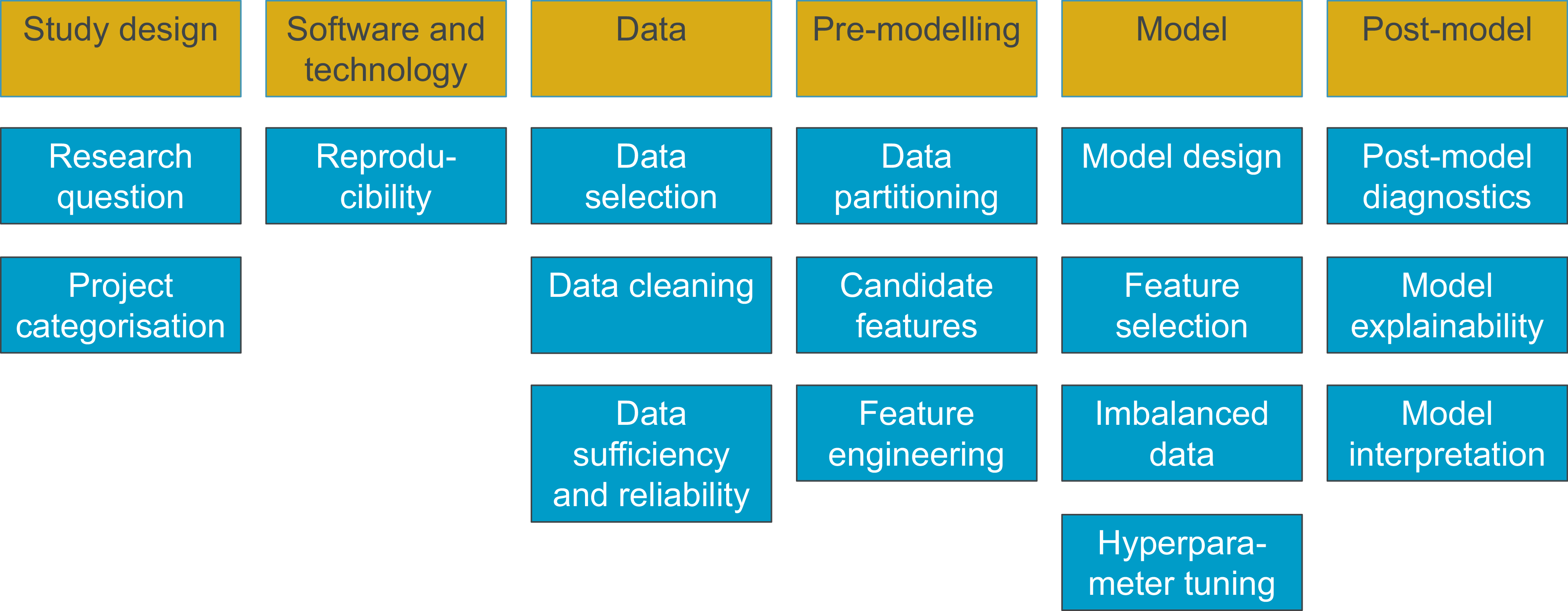
We structured the checklist in a way that would follow the natural flow of an actuarial research project. Figure 1 shows the main headings, and for each heading, there are one or more topics that are discussed in the framework. That would be in the form of a write-up, with some of the most useful concepts, recommendations and citations for future reading included. The framework itself is available via the IFoA website, so everything can be accessed for download and reading.
Framework structure.

We talk through some of the topics in the framework. Fiona (Fan) will start by covering data cleaning and imbalanced data.
Ms F. Fan, F.I.A.: I will start with data cleaning. It is normally one of the first steps when we start our analytics projects. I will focus on how we handle missing data and outliers. Handling missing data is what we do in our day-to-day life, because our data are not perfect. I have three ways of handling it, assuming we do not want to discard the data. Sometimes we have missing cells, and we want to keep some of the rows. We can fill in the missing cells with median or mean values, and this is a simple and easy technique. It is easy to understand. However, if the rest of the data is not representative of the missing data, then it can introduce some bias. An alternative method uses multiple imputation chain equations (MICE). A third option is a random forest technique, but I will not go into that in detail.
One of the key things to bear in mind when we are handling missing data, and sometimes outliers, is that the missing data is often not random, so whichever technique we choose, we might introduce bias. There is no universal fix. The first step is always to understand why the data is missing, and if possible, to go back to the data source and look for the data. I also want to note that some models can handle missing data directly. For categorical data, one effective approach is to add an “unknown” category. It is important to note that sometimes blank cells and null cells mean different things, and they should be treated separately.
There is always a question of how much missing data we are comfortable dealing with. It has always been a debate, but we feel that if more than 25% of the data is missing, then any techniques need to be used with caution, because accuracy will drop. The strategies for handling missing data work best with data that is missing completely at random or missing at random. For example, if you have data coming from your underwriting or claims team, and there has been a data glitch that arose from an accident, then that data is missing at random, and we can deal with that. However, when data are missing not at random, for example, if a policyholder chooses not to disclose pre-existing medical conditions, then it is harder to fix, and there is a likelihood of bias.
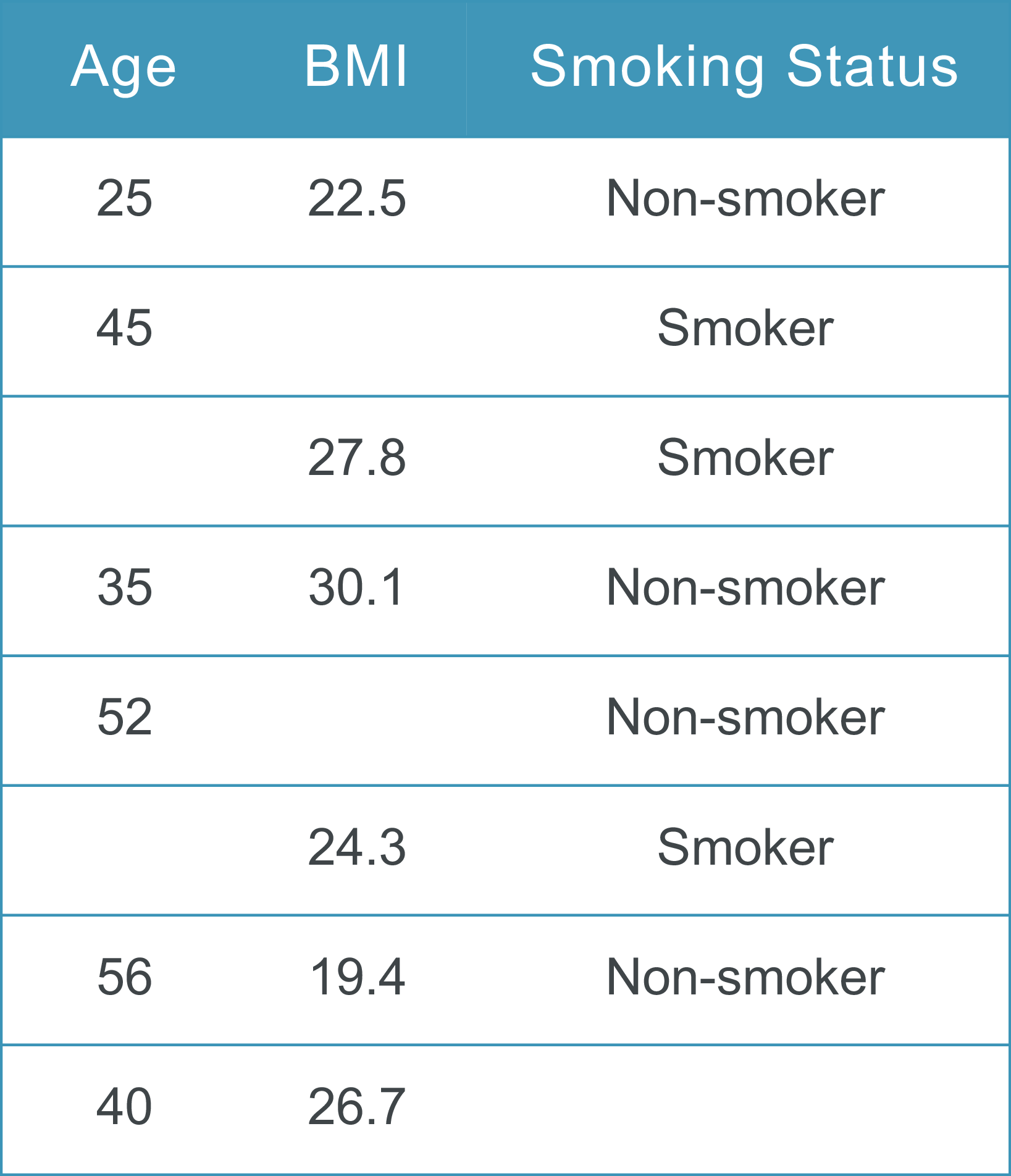
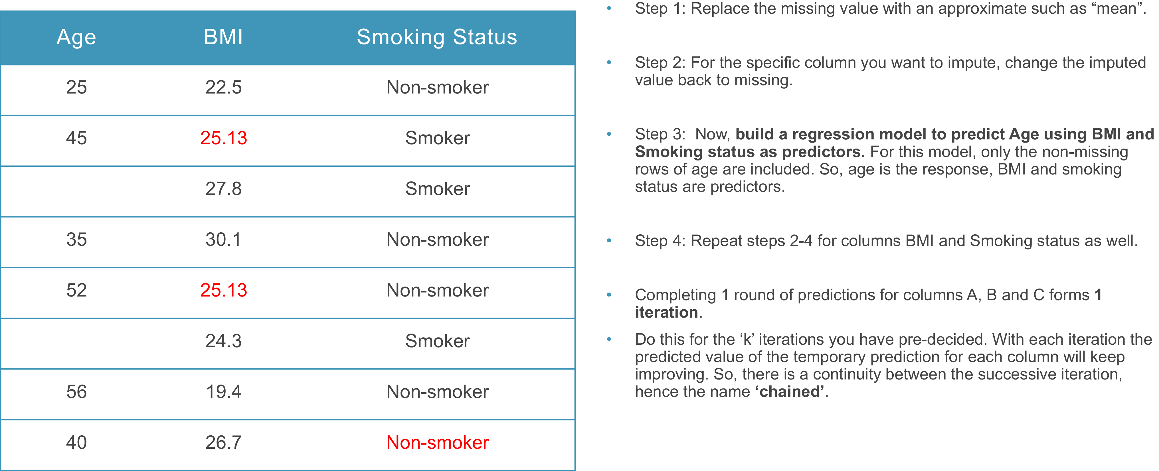
I have a very simple example of missing data to demonstrate the MICE method. In Figure 2, I have eight made-up model points with some cells missing. The data includes age, body mass index (BMI) and smoking status. The first step of the MICE technique is imputation, and it replaces the missing values with approximate values (Figure 3). For the missing ages and BMI values, averages are used. For smoking status, because non-smokers appear most of the time, the model guesses that this cell is going to be a non-smoker.
Missing data.

MICE.

Then, taking each column in turn, return the imputed values to missing and build a regression model to predict the missing values. For example, if you start with age, you remove the estimated age values and predict age using the BMI and smoking status as predictors. In this example, rows one, two, four, five, seven and eight would be used to predict the missing cells in age. That process is repeated for BMI, and rows one, three, four, six, seven and eight would be used to predict the missing cells. The process is then repeated for smoking status. This completes the first iteration. We complete a pre-defined number of iterations. With each iteration, the predicted value will keep improving, and there is continuity between each iteration, which is where the “chain” in MICE comes from.
Next, I cover imbalanced data, which fits within the modelling techniques heading. Imbalanced data present a very common challenge. A classic example is detecting rare events, for example, fraudulent claims, or in medical statistics, diagnosing a rare disease. In the case of fraud, the minority class would be fraudulent claims, and the majority class would be legitimate claims. In our data set, we have a lot of legitimate claims and very few fraudulent ones, but we want to detect the fraudulent ones. The imbalanced data can mislead models into always predicting “not-fraud” to achieve very high accuracy. This is very dangerous. The cost of failing to detect a fraudulent claim is significantly higher than the cost of incorrectly flagging a legitimate one. While flagged cases can be reviewed and resolved through investigation, an undetected fraudulent claim can result in substantial financial losses for the insurer.
There are different methods for dealing with this problem. The data-level methods are resampling techniques: oversampling the minority class, undersampling the majority class and hybrid methods that combine both. There are algorithm-level methods where we can apply a class weighting to give more importance to the minority class. This makes the model pay more attention to the fraudulent claims, which is very important for false negatives. We need to use different metrics correctly, so, for example, precision is how many predicted frauds are fraudulent, and recall is looking at how many fraudulent cases we caught. An F1 score lies between those two metrics.
I have a very simple example of imbalanced data. I generated an artificial data set of insurance claims in R. About 4% of claims are fraudulent. In Figure 4, the chart shows the legitimate claims as red dots and the fraudulent claims as green dots. You can see that the majority class outweighs the minority class. We want to build a model that predicts fraudulent claims. I fit a generalised linear model (GLM) to this data set, and it predicts that 100% of the claims are legitimate. The results give very high accuracy, because the model was right 959 out of 1,000 times. However, it is of no use because it did not predict any fraudulent claims.
Imbalanced data example – simple model.

I then completed some data manipulation. I simulated oversampling by generating 901 synthetic samples. This increased the minority class. Previously, we had 959 legitimate claims and 41 fraudulent claims. This generated another 901 fraudulent claims to make the data more balanced, and then I trained another GLM on that data set. This GLM predicted 20 fraudulent claims, and so it performed better than my previous GLM.
I have an example of how this works. In Figure 5, the chart on the right-hand side shows the oversampling. The green dots that did not appear in the chart on the left, i.e. the newly generated ones, were between the original minority cases. You cannot see any generated green dots in the top right corner because there were none in the original data. The model is trying to mimic the behaviour of the minority class.
Method A – oversampling comparison.

The next method is undersampling. In contrast to oversampling, where we increase the minority class, here we reduce the majority class. You can see in Figure 6 that we have 41 fraudulent claims and 41 legitimate claims. I fit another GLM onto this data set, and it predicted 26 true positive frauds. This prediction was better than the prediction of the oversampling GLM, but it predicted many more fraudulent cases overall. For the legitimate claims, it predicted 560 fraudulent claims. This is something we can tolerate. It is possible to investigate the legitimate claims, but we do not want to miss fraudulent claims.
Oversampling and undersampling comparison.

Figure 6 shows a comparison between different degrees of data-level resampling. The chart on the left is what we started with, a very imbalanced data set: The majority class outweighs the minority. In the centre, on the top, we have the undersampling data set, where we reduced the majority class. At the bottom in the centre, we have the oversampling data set, where we increased the minority class: Our aim was to make the data more balanced. On the right, I have the data set from a hybrid method, where I reduced the majority class and also increased the minority class to make the model focus more on the minority class.
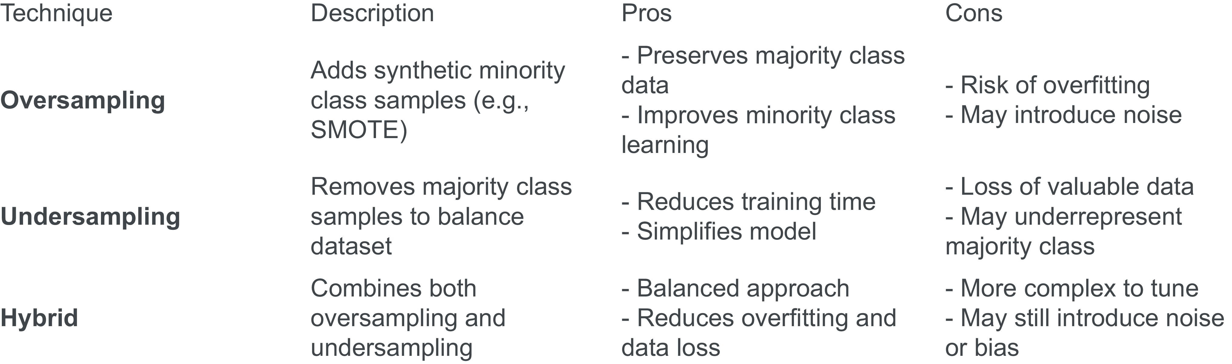
Figure 7 shows a comparison of the different methodologies. Oversampling adds synthetic minority samples, so it is great for improving the learning, but it can also have the risk of over-fitting and adding some noise. Undersampling removes the majority of samples, so it speeds up training and simplifies the model, but we might lose some valuable data in the majority class. The hybrid method combines both, but it requires more tuning. It offers a balanced approach, but it can be quite complex, and it can still introduce bias.
Data-level method comparison.

Mr J. Tam: I am going to talk about pre-modelling and the model. Specifically, I am going to focus on feature engineering and model design. I will start with feature engineering for numeric variables. The key objective here is to enable the model to capture non-linear relationships with the target. This step is essential for GLMs as they cannot learn non-linear relationships from the data. Most machine learning (ML) models should be able to capture non-linear relationships on their own, but this step is still beneficial as it enables the model to learn genuine patterns in the data.
I will walk through three methods that I think are helpful for feature engineering the numeric variables. The first one is polynomials. An example of this is using BMI to predict sickness incidence. We know that being either underweight or overweight increases the risk for policyholders. By creating and introducing a quadratic term for BMI, we can capture the parabolic relationship, especially for GLM modelling. The second method is trigonometric functions. These enable us to learn cyclical patterns. An example here is demand cycles, which tend to fluctuate on an annual basis. By introducing sine and cosine transformations of the day of year, we can, in theory, learn any shape of the demand cycles. The final method that I find useful is bucketing, i.e. transforming continuous numerical variables into ordered groupings. An example here is a sum-assured band, which we know tends to cluster around round numbers, for instance, 50,000, 100,000 or 250,000. By banding the continuous assured amounts into ordered bands, for instance, 0–50,000 and 50,000–100,000, we can reduce noise and manage the outliers.
To illustrate the different ways of featurising categorical variables, I am going to use an example of smoker status in the context of mortality modelling. One method is One-Hot encoding, where we create one indicator variable for each category. A second method is Dummy variable encoding, which is very much akin to One-Hot, the only difference being that we drop the indicator column for the base category. Here, we create n − 1 columns for n categories. A downside of One-Hot and Dummy encoding is that we are creating multiple columns for one categorical variable. This will be problematic, especially when the number of categories is high, and that is where Target encoding comes into play. Target encoding essentially uses the average target level to encode a category. The result is one numeric column representing the entire categorical variable. The downside is that we are essentially using the target information to predict the target, which means that there will be target leakage. One way to get around this is using cross validation. For instance, if we split the training data into two folds and we use the target information from one fold to encode the other, it can eliminate data leakage.
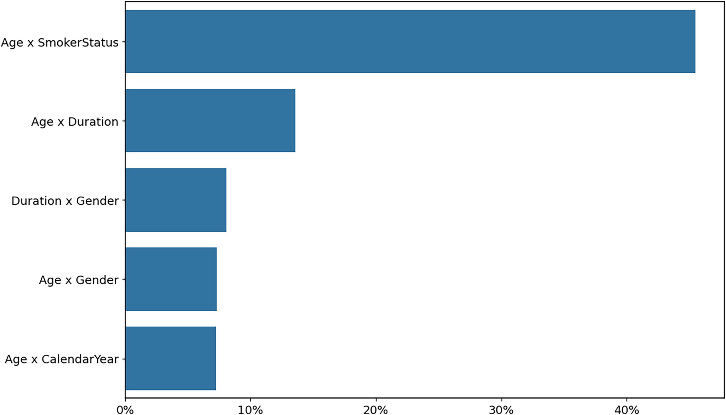
We know that most ML models are able to capture feature interactions natively. GLMs and additive models usually cannot learn feature interactions. In the past, interaction detection depended heavily on domain knowledge. Nowadays, with the advancement of data science, we can use a gradient boosting machine to detect interactions automatically. One way of doing this is to first create a baseline model that contains just the individual effects. We then train Gradient Boosting Machines (GBMs) to identify interaction effects by training the model to predict residuals from the baseline model. Once we have identified all of the top interactions, we incorporate them back into the additive models. In Figure 8, the chart shows the interaction importance that we have detected. We can see that age versus smoker status is by far the most important interaction term. By incorporating this into our additive model, we can see the model trend shown in Figure 9. The excess mortality of smokers increased with age when compared with non-smokers. This is consistent with the empirical observation in the mortality statistics compiled by the Continuous Mortality Investigation (CMI).
Identified interaction importance.

Top interaction model trend.

Next, we move on to model design. The problem statement for modelling is that, usually, we have a data set with input variable X and output variable y, and the relationship between X and y is based on a mechanism instigated by nature. There are two modelling cultures. The data modelling culture represents traditional statistical thinking. Here, what we want to understand is the conditional distribution of y given X. There are a number of tools that we can use to do this kind of modelling, for example, linear or logistic regression or the Cox survival model. The advantage of this is that it is very interpretable, but the drawback is that it tends to rely on some very strong assumptions. Alternatively, the algorithmic modelling culture represents the engineering-style ML modelling. Here, we are less concerned with understanding the conditional distribution of y given X. We are more interested in building predictive models, where we can use X to predict y. Examples of these are tree-based models and neural networks. These models are very flexible, which means that they can capture complex relationships, but the downside is that they operate more like a black box.
The question is, can we have the best of both worlds? There are two aspects here. First, we can use ML algorithms to improve our GLMs. I have already talked about using gradient boosting machines to detect variable interactions. Also, we can build ML models to visualise non-linear relationships, so we know which polynomial terms to add to GLMs to enhance their predictive power. On the other hand, we can make the ML models more interpretable. I want to highlight that actuaries are very much involved in the development of explainable neural networks, tailored for actuarial applications. These kinds of neural networks tend to avoid over-fitting and are also more explainable.
How do we build explainable GLMs? We need two functionalities. Interaction constraints enable us to enforce additive structure by limiting feature interactions, and continued model training allows us to build on existing models incrementally. Both XGBoost and LightGBM support these functionalities. We can use a two-step approach to develop a GBM model. First, we create a base model with no interactions allowed, which means each tree is based only on one variable. Second, we add pairwise interactions via continued training from the base model. Here, the pairwise interactions are added only when the residuals cannot be explained by individual effects alone. As a result, the GBM will be more explainable, as it has much clearer model trends.
Mr J. S. Minhas, F.I.A., C.Act.: I will be talking about post-model diagnostics. This refers to the steps or techniques used to assess our model’s reliability and performance. After we have built our model, it is important to verify that it performs well, not just on training data but also on unseen data. This is crucial for real-life applications as we want to avoid over- and under-fitting. When we build models, we will often rely on various assumptions, such as the independence of errors or constant variance. If these assumptions do not hold up on unseen data, our results will likely be biased or misleading. Post-model diagnostics help us to identify these issues early on. We also want to make sure that our model performs well on training data. For example, we might train a model, and it might look good statistically, but it may fail to meet our business needs. A typical example is that large language models (LLMs) might perform quite well on benchmarks during training, but they may fail to add value in business cases. Post-model diagnostics help us to identify whether our models are fit for purpose. From a governance perspective, post-model diagnostics help to justify our model selections and provide evidence to audit our model’s robustness and reliability.
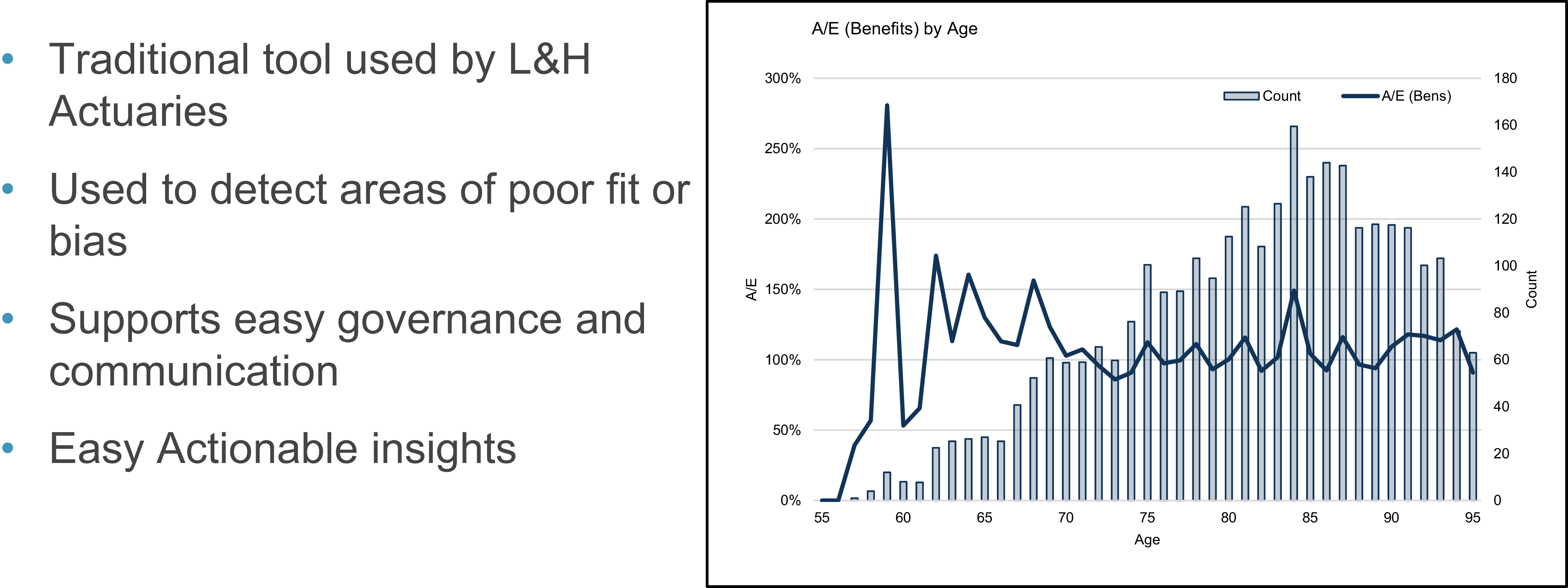
A traditional method used by life and health actuaries to assess goodness of fit is the A over E graph. We plot our actual experience against the expected experience predicted by our model, against a feature. Figure 10 shows a univariate graph, and in this example, we have age on the X axis. These graphs are quite simple and intuitive. You can use them to quite easily understand whether we have poor fit or bias against particular features. They support simple governance and easy communication for stakeholders, and it allows us to create simple and actionable insights. For example, in Figure 10, our fit looks quite good from the age of 70 onwards, but you can see that our fit is not as good at the younger ages. This might point out an area to explore, and our model might be recalibrated accordingly.
A/E (benefits) by age.

Figure 11 shows a double lift graph. This is a popular tool used in personal lines insurance to compare a new model to an existing or baseline model. The core idea is to segment the data by the ratio of the predictions made by the two models, then examine which model tracks better with our actual observations. It helps us to identify model performance across deciles and risk classes. For example, you could stratify these graphs by some assured banding or another factor. Figure 11 is from Michiel (Luteijn)’s and Jackie (Tam)’s case study, which was published in The Actuary magazine in July/August 2025. They built a Generalised Additive Model (GAM), and on the X axis, we have the ratio of the GAM prediction to the baseline CMI model. On the left-hand side of the X axis, we have predictions where the GAM predicts lower mortality, and then on the right-hand side, we have predictions where the GAM predicts higher mortality. We then plot the GAM curve, as well as the CMI model curve, and compare it to the actual observation curve in blue. You can see from the left-hand side of the plot, where the GAM predicts lower values, the fit tracks very closely to the actual observations, suggesting that the GAM is better fitted than the CMI model. On the right-hand side, it is less clear, but the actual observations seem to track slightly closer to the GAM, suggesting a better fit again.
Double lift – GAM predictions to CMI mortality table.

Another graphical approach that could be used is learning curves. These are typically used to assess the performance of learning models, such as neural networks or gradient boosting machines. They can be used to detect over- and under-fitting. Figure 12 shows an example graph looking at a gradient boosting machine model. On the X axis, we plot the number of trees, and on the Y axis, we plot our deviance loss. The plot has two curves, one for the training data set and one for our validation set. In this instance, if the training error is low, but the validation error is high, that might suggest over-fitting. In instances where both the training and validation errors are high, that might suggest under-fitting.
Deviance loss by number of trees (XGBoost).

Moving on to model explainability, I will start by outlining why this might be important. Regulatory frameworks and internal risk models might require our models to be explainable and justifiable. It can also help to build trust and confidence with key stakeholders such as senior management or regulators. Explainable models help us to reduce the risk of bias and discrimination. For example, we might use model explainability techniques to ensure that certain protected features, such as gender or race, are not driving model predictions. It can also be used for customer justification; for example, it can allow us to explain premium increases. Model explainability is also important for risk management. An explainable model increases transparency and should result in a lower risk of unexpected behaviour in our model output, and it should also allow for easier monitoring and recalibration when models change.
One technique that is widely used is feature importance. Feature importance measures how each input variable contributes to the model output, and it helps us to understand which factors are driving the model output. One such example is permutation importance. This is a particularly popular method, as it can be used for any type of model. It involves randomly shifting values for a feature and then measuring the impact on the model’s prediction. For gradient boosting machines, feature importance can be measured by measuring the model improvement attained when adding a variable during model training. Feature importance can also be used in feature selection. For example, we could create a gradient boosting machine to identify the most important features and then use these features to build a simpler and more explainable model, such as a traditional GLM. This is illustrated in Figure 13.
Factor strengths.

Another example is SHapley Additive exPlanations (SHAP) values. These can be used to help increase model explainability. They are based on co-op game theory and used to increase transparency and interoperability of our models. In the example in Figure 14, we are plotting SHAP values on the X axis against various features. Looking at the commencement year feature, as we go from low to high values, the SHAP values show that our prediction shows lower A over E values. That might be due to changes in underwriting or changes in product features.
SHAP importance plot.

Dr Luteijn: I will cover model interpretation. Why do we need model interpretation? Once we have detected an association between exposure and an outcome, how can we be confident we have identified a causal relationship? I would argue that this is quite important. What is the problem here? There is a great example from epidemiology. As we know, smoking causes lung cancer. However, smokers are also more likely to drink coffee. So, if we were to have a data set without smoking information, but with coffee drinking information, we would find a relationship between coffee drinking and lung cancer. Without model interpretation, we may incorrectly conclude that coffee drinking causes lung cancer, but this is obviously a confounding factor. There are many examples from insurance. One example that I can often find in data sets is that level policies often have higher smoking rates than decreasing policies. If we did not have access to smoking information in our data, some of the increased mortality due to smoking could incorrectly be attributed to level policies.
In some cases, there could be an argument for using proxy variables for modelling claim experience. For example, the sum assured itself does not directly affect mortality risk, but can be used as a proxy to price for variables we may not have access to, such as conscientiousness. However, even in these cases, it is useful to at least be aware of the variable being a proxy.
There is a framework from medicine that can be used to determine whether a relationship is causal, called the Bradford-Hill criteria. Once a model has been fit, these criteria could be used to determine whether any detected relationship is causal. The first criterion is relationship strength. If the hazard ratio or relative risk, or whatever metric we are using in our model, is larger, that increases the probability that the relationship between the exposure and the outcome is real. The second criterion is consistency. For any relationship we find, if we can find it in different populations (e.g. urban and rural populations, older and younger lives or males and females), that makes it more likely that it is a real relationship between exposure and outcome. The third criterion is specificity. If the exposure causes a very specific critical illness, it makes it more likely that it is a real effect. An example is asbestos exposure, which causes a very specific type of cancer.
The fourth criterion is temporality. This one is a bit obvious, because of course the exposure must precede the outcome. The fifth criterion is the biological gradient. As we know, smoking causes lung cancer, and drinking alcohol increases the risk of liver conditions. But within the exposure group, there is a gradient. Light smokers have a higher risk of lung cancer than non-smokers, but heavy smokers have an even higher risk of lung cancer than light smokers, and similarly with alcohol. That is a biological gradient, or dose response, and that makes it much more likely that this is a real association. The sixth criterion is plausibility. There needs to be a credible mechanism between cause and effect. An example would be between smoking and lung cancer. If smokers have a higher risk of broken bones, that may raise some concerns around whether this is a real association, because there is no clear mechanism of action. For lung cancer, there is an obvious mechanism of action, because the smoke enters the lungs, where it is quite conceivable that it causes damage, and therefore increases the risk of lung cancer.
There are three more criteria. The next is coherence. The cause and effect should not conflict with generally known facts. For example, it is generally known that more affluent lives have a lower risk of mortality. Therefore, we would expect that larger sums assured would have a lower risk of claims than smaller sums assured. If we were to find in a data set that the opposite is true, that would warrant further investigation. Likewise, if we were to find lower mortality claim incidence among smokers, that would also conflict with prior knowledge. The eighth criterion is experiment. If the exposure is switched on or off, then you would expect the risk of the outcome to change accordingly. A great example here is the A/B testing for sales online, or perhaps lapse rates. If we changed certain elements of the sales process, and the lapse rate changed, and we change it back, and the lapse rate goes back to where it was before, that makes it more likely that there was a real relationship there.
The last one is analogy, meaning similar factors suggest similar effects. As we know, smoking causes lung cancer. So, if e-cigarettes also increase the risk of lung cancer or lung conditions, the evidence there is stronger, because it is analogous to cigarette smoking. There is a strong reason to believe that similar causes have similar effects, so this would be a real effect. Those are the Bradford-Hill criteria. They are useful for assessing whether statistical correlations between exposure and outcome are just noise or something real.
We have covered some parts of the framework in terms of technical content, but we did not cover the entire framework. Within the topics that we did cover, we did not exhaustively cover what is in the framework. With this framework, we aim to enhance transparency, reproducibility and comprehensiveness in analysis. We hope that it can support not only conducting but also reporting on analytical projects, because the layout lends itself nicely to a structure for a write-up, as well as peer review. We did have some challenges defining the scope for the framework. For example, we decided to exclude generative AI and large language models. They are becoming increasingly important, and there is a lot of interest in the topic. We felt that we did not have the background to properly include it in the framework and justify the importance of the topic. As it is, at the moment, not widely used for analysing tabular data, we felt that it was out of scope.
The second challenge is that this is a rapidly evolving landscape. The framework today may become outdated over time as the data science field and generative AI grow, not only in technical terms but also in terms of adaptations in the actuarial field. The Department for Education produced a report, two years ago now, that said that the finance and insurance sectors are the most exposed to disruption by AI. This illustrates the point that we are living in a very rapidly evolving landscape.
Now we move to the question-and-answer session.
Question: When it comes to, for example, more sophisticated algorithms, how could you use something like a black box algorithm to improve more transparent models, such as GLMs?
Mr Tam: First, we can use a gradient boosting machine to detect interaction effects, which we can plug back into GLM or additive model training. We can also use GBM to visualise any non-linear relationships between the target and input variables, so that we can infer the most appropriate polynomial terms to add to the data set. Another approach is to train GLM on GBM model predictions. This is predicated on GBM predictions being more predictive than GLM ones and allows us to capture, say, about 80% of the GBM benefit without compromising model interpretability. This is a useful technique – if underwriters or actuaries are not too confident using or implementing GBMs, we can just train GLMs to predict the GBM output, which results in more predictive GLM models.
Question: I found the section on the imbalanced data interesting and actionable. I am interested to know why class weighting wasn’t explored.
Ms Fan: Class weighting has good benefits. Just in the interests of time, I did not explore further in this talk. The example I generated also used class weighting, and it outperformed the data-level resampling adjustments. Class weighting can be advantageous if your stakeholders are not comfortable with reducing or increasing the amount of data using synthetic data points. In class weighting, you tell the model to increase the weight of your minority class. For example, if your minority class case is twenty times less than the majority class, you can tell the model to focus on the minority class twenty times more. That has its own benefit, as you do not touch the data at all. It is a method that I would recommend that you explore when you are doing your modelling.
Question: In the section on model explainability, in Figure 12, feature importance is plotted on the X axis. The percentage for age exceeds 100%. How is that possible?
Mr Minhas: On the X axis, we plotted the standard deviation of relativities associated with each variable, which is why it is possible to go above 100% for age.
Question: This is a cross-disciplinary working party, what was the most surprising finding for you?
Dr Luteijn: One of the concerns we had at the beginning was whether the work had already been done. However, very little has been done in this area. I know that the IFoA has quite a large interest in applying data science to actuarial work, but there was no framework for this as such. I feel that most people are trained in one discipline. There are a number of actuaries with expertise in data science, but other fields such as software engineering and epidemiology can offer great benefits and provide a view of the larger picture. There are not many people who have expertise that overlaps all of those disciplines, but it feels like there is a lot of opportunity for actuaries to leverage concepts from other fields, such as the Bradford-Hill criteria. I was surprised by how little has been done so far and how many benefits there are to be gained.
Question: You have looked at lots of different model types here. In your day-to-day work in life and health insurance, what do you find better, LightGBM, XGBoost, CatBoost or something else?
Dr Luteijn: I generally use LightGBM because it is quicker than the other two. From my understanding, XGBoost is better out of the box, so it may have better performance without too much effort. CatBoost is rather slow, but as per its name, it is very good with categorical features.
Mr Tam: Yes, I agree with you. LightGBM tends to work best when there is a lot of data. It grows trees leaf-wise, which means the model is fairly flexible in learning complex relationships. CatBoost, on the other hand, works well with small data sets. It uses a symmetric tree structure, which is a way to control model complexity. XGBoost tends to be easier to use, so I use it for most modelling tasks.
Question: I appreciate that gen AI was not in scope of the working party, but there are a lot of process-driven steps, such as the data cleaning and feature engineering. Do you think gen AI will have an impact on speeding up some of those data cleaning or feature engineering steps?
Dr Luteijn: I find it most useful for writing code. I have my favourite packages for doing various jobs, but I may have a bit of tunnel vision, because I am mainly exploring solutions using those favoured packages, whilst another tool could be better suited for certain situations. An example of that is that I mainly use the data. Table R package, as opposed to the Tidyverse. Generative AI is unbiased, so it does not have that preference that I have. It helps with finding new ways of doing things. For the analytics itself, I have not found it equally useful for tabular data. From my understanding, the benefit of gen AI and neural nets and those technologies is for more complicated data, with more than two dimensions (beyond just rows and columns), so non-tabular data.
Mr Tam: I agree that Gen AI, especially LLMs, is more useful for understanding unstructured data. One of the use cases in actuarial modelling is engineering structured features from unstructured data, for instance, medical records for patients. We can ask an LLM to extract times or dates of diagnosis, the results of diagnostic tests or even a patient’s medical history, all of which can be turned into useful, structured features that can enhance actuarial models.





 Open access

