Introduction
The West African Dwarf (WAD) sheep (Rege, 1992) constitute the most important indigenous sheep breed found in the humid region of Africa, where trypanomosis and worm diseases impose a significant constraint. In Benin, the WAD sheep is raised exclusively for meat and was estimated at 700 000 (Faostat, 2005), and play an important economical, social and cultural roles. For this purpose in West and Central Africa, the genetic and non-genetic effects on the growth performance of WAD sheep had become an attractive study in last decades to improve overall productivity (London and Weniger, Reference London and Weniger1995; Yapi-Gnaoré et al., Reference Yapi-Gnaoré, Oya, Rege and Dagnogo1997; Gbangboche et al., Reference Gbangboche, Adamou-Ndiaye, Youssao, Farnir, Detilleux, Abiola and Leroy2006a and Reference Gbangboche, Youssao, Senou, Adamou-Ndiaye, Ahissou, Farnir, Michaux, Abiola and Leroy2006b). However, the advantage of growth models such as Logistic and Gompertz (Renne et al., Reference Renne, Langhammer, Wytrwat, Dietl and Bunger2003; Lambe et al., Reference Lambe, Navajas, Simm and Bunger2006), Von Bertalanffy (Topal et al., Reference Topal, Ozdemir, Aksakal, Yildiz and Dogru2004) and Brody model (Bathaei and Leroy, Reference Bathaei and Leroy1998), which give an explanation of what is biologically occurring during the growth phase of an animal, and their importance on breeding program (Varona et al., Reference Varona, Moreno, García Cortés and Altarriba1997; Lewis and Brotherstone, Reference Lewis and Brotherstone2002) were unknown in WAD sheep. Therefore, model selection to predict typical growth in livestock industry, became a daunting task, given the broad range of criteria for goodness of fit, as the Akaike’s Information Criteria (AIC) (Akaike, Reference Akaike1974), the coefficient of determination (R 2), the mean squares errors (MSE), the log-likelihood (lnL) values, and the least average prediction error (APE) (Brown et al., Reference Brown, Fitzhugh and Cartwright1976; Goonewardene et al., Reference Goonewardene, Berg and Hardin1981; Beltran et al., Reference Beltran, Butts, Olson and Koger1992; Lambe et al., Reference Lambe, Navajas, Simm and Bunger2006).
At least 800 head of WAD sheep were yearly maintained in the Bétécoucou breeding farm in Benin. Measuring the weight using spring balance becomes a long and difficult work due to the increasing number of animals. The knowledge of the adapted growth curves for WAD sheep in this farm should be helpful in determining proper management and in implementing selection decisions. Therefore, the objectives of this study were to compare the goodness of fit of non-linear function (Von Bertalanffy, Logistic, Gompertz and Brody) and to provide a specific shape of the growth curve according to the environmental effects on monthly weight from birth to 180 days of age in WAD sheep.
Material and methods
Animal and management
The WAD sheep is a small mature size hairy breed found all over West and Central Africa to the south of 14° latitude, and is widely distributed throughout the savannah and humid zones under tsetse-infested areas (Epstein, Reference Epstein1971; Rege, 1992). The WAD sheep is a compact breed with a short horizontal lop ears. The rams are horned and females usually polled. The coat color varied from spotted black and white to solid black or white. Mature size ranged from 40 to 60 cm at withers, mature weight from 20 to 30 kg for dams and from 25 to 35 kg for rams (Charray et al., Reference Charray, Humbert and Levif1992; Gatenby, Reference Gatenby2002).
The Betecoucou breeding farm is situated in the Soudano–Guinean zone of Benin (between 2°20′ to 2°28′E longitude and 7°45′ to 7°52′N latitude) and was the reference center that provides superior animals to the sheep farmers. The year comprises two seasons: the rainy season from March to October and the dry season from November to February. The lambs are born during the year with a peak in rainy season. The new lambs were kept with their dam until weaning (90 days). Post-weaning male and female lambs grazed separately on the cultivated and natural pastures, and had no access to supplement other than that offered to the dams. The age at first lambing is between 430 and 838 days and the lambing interval, 190 and 544 days. The birth weight within 24 h of birth was taken using a platform type dial balance (10 kg capacity with 0.05 g accuracy). The weaning and post-weaning weights were recorded using a suspended spring balance (50 kg capacity with 200 g accuracy). The birth weight, weaning and 180-day weights were the criteria of selection. Management of the flock was described by Gbangboche et al. (Reference Gbangboche, Adamou-Ndiaye, Youssao, Farnir, Detilleux, Abiola and Leroy2006a).
Data and preliminary environmental effect analysis
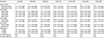
Monthly weights of WAD lambs from birth to 6 months (180 days) of age were provided by the Betecoucou breeding farm. The dataset consisted of 5274 records of 889 lambs, from year 2001 to 2004, born as single or double from 1st, 2nd and 3rd dams parity, during the dry and the raining seasons. The General Linear Model Procedure (proc GLM) of the Statistical Analysis Systems Institute (SAS, 2002–2003) was applied to the data to identify the significant effect of some environmental factors on the observed live body weight.
The fixed model used was:

where Yijklmn is the adjusted weight of the nth lamb, μ is the overall mean, Si is the fixed effect of the ith sex (i = male, female), Tj is the fixed effect of jth year of birth (j = 2001, 2002, 2003, 2004), Uk is the fixed effect of kth season of birth (k = dry season, rainy season), Vl is the effect fixed of lth birth type (l = single, twin), Wm is the effect fixed of mth parity (m = 1, 2, 3), Eijklmn is the random error attributed to the nth lamb. Statistical differences between means were compared using Student’s t-test. The number of observations, description of environmental factors and the least-squares means of live body weight are summarized in Table 1.
Number of observations in parentheses (), least-squares mean ± standard error (LSM ± s.e.) of monthly weight from birth to 180 days of age, the level of significance of fixed effects, the coefficient of determination (R 2) and the coefficient of variation (CV) indicated by the proc GLM

BW, W30, W60, W90, W120, W150 and W180 were birth, 30, 60, 90, 120, 150 and 180 days weight, respectively. *P⩽0.01; **P<0.001. Within a column (and within each factor), values with different superscript letters differ significantly at P < 0.05.
Models and goodness of fit
The Logistic, Gompertz, Von Bertalanffy and Brody functions were fit to the data to model the relationship between weight and age. The Logistic and Gompertz models have been described previously (Renne et al., Reference Renne, Langhammer, Wytrwat, Dietl and Bunger2003) for the Brody (Bathaei and Leroy, Reference Bathaei and Leroy1998) and for Von Bertalanffy (Topal et al., Reference Topal, Ozdemir, Aksakal, Yildiz and Dogru2004). These models can be specified as:
Brody (exponential),

Gompertz (sigmoid),

Logistic (sigmoid),

Von Bertalanffy (sigmoid),

where Wt is the observed weight at age t expressed in months, and A is the asymptotic limit of the weight when age (t) approaches infinity. This does not imply that A is the heaviest weight attained by the individual, but it indicates the average weight of the mature sheep, independent of short-term fluctuation in weight due to temporary environmental effects. B indicates the proportion of the asymptotic mature weight to be gained after birth, established by the initial values of W and t. k is a function of the ratio of maximum growth rate to mature weight, normally referred to as maturing rate. It is related to postnatal rate of maturing and serves both as a measure of growth rate and rate of change in growth rate. Large k values indicate early maturing animals, and vice versa, e is Napier’s base for natural logarithms, t is age expressed in day.
The language of technical computing package of Matlab®, 2006 was used to calculate the least-squares estimates ± standard error of the models parameters (A, B and k), the R 2, the MSE and the AIC. Details about the computing in Matlab®, 2006 are described in the Appendix.
The goodness of fit was assessed by using the higher R 2, the lower MSE and AIC values (Brown et al., Reference Brown, Fitzhugh and Cartwright1976; Akbas et al., Reference Akbas, Taskýn and Demirören1999; Topal et al., Reference Topal, Ozdemir, Aksakal, Yildiz and Dogru2004; Lambe et al., Reference Lambe, Navajas, Simm and Bunger2006). Even though the selected models provide a view of the predicted weight at fixed age, the parameters A, B and k of the significant effect of season of birth, sex of the lamb, the parity of dam, the type of birth and the year of birth on the observed weight, have been calculated separately (Matlab®, 2006) simulating specific slop of the selected growth curve.
Result and discussion
Model parameters
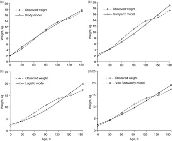
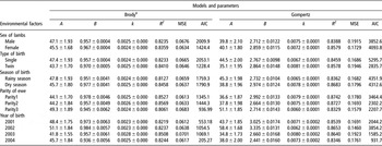
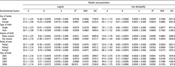
The least-squares estimates parameters A, B and k, the R 2, the MSE and the AIC of the four competing models were reported (Table 2). The Figure 1 shows the pattern of each model from birth to 180 days of age: the Brody model was typically exponential (Figure 1a), while Gompertz (Figure 1b), Logistic (Figure 1c) and Von Bertalanffy (Figure 1d) models classically sigmoid. The parameter A was maximum in the Von Bertalanffy model (62.5 kg) and considerably less in Logistic model (31.0 kg). The estimate of B was smaller in the Von Bertalanffy (0.658 kg), while Gompertz (27.994 kg) showed greater values. The growth rate k, range from 0.0024 to 0.0174, showing the early maturity rate in Logistic model than other. When applying Brody growth function for the Mehraban Iranian fat tailed sheep, Bathaei and Leroy (Reference Bathaei and Leroy1998) reported values 70.02, 0.95 and 0.1195 for A, B and k, respectively. Similar to this study, Brown et al. (Reference Brown, Fitzhugh and Cartwright1976), Goonewardene et al. (Reference Goonewardene, Berg and Hardin1981), Rogers et al. (Reference Rogers, Pesti and Marks1987) and Goliomytis et al. (Reference Goliomytis, Panopoulou and Rogdakis2003) obtained different A, B and k values when fitting different growth functions to the same weight–age data indicating that the model of choice affects parameter estimates.
Parameters estimates ± standard error, coefficient determination (R 2), mean square error (MSE) and Akaike’s Information Criterion (AIC) of four models describing the growth curve in West African Dwarf sheep and the parameters related to the shape of the environment factors in the selected Brody model

‡Selected model: A is the predicted asymptotic weight at maturity (kg), B is the proportional difference between A and birth weight (kg) and k is the rate of maturating.
The shape of Brody (a), Gompertz (b), Logistic (c) and Von Bertalanffy (d) growth models v. observed monthly weight from birth to 180days of age in West African Dwarf sheep.

All competing models in this study had high R 2 from 0.82 to 0.84, suggesting overall good fits to the data. According to R 2 values models fall in the order Von Bertalanffy > Gompertz > Brody > Logistic. The MSE value ranged from 0.0662 to 0.4557 and the Brody was ranked 1st according to the lowest MSE value. AIC values used to compare models, provide the following rank: Logistic > Gompertz > Von Bertalanffy > Brody, implying that the Brody model had the least AIC value. Various R 2 and MSE values have been found in the literature, depending on the model applied, the structure of dataset and the species of animal. Higher R 2 values (0.98 to 0.99) and MSE (2.1 to 3.2) were reported for Morkaraman and Awassi lambs (Topal et al., Reference Topal, Ozdemir, Aksakal, Yildiz and Dogru2004). In the Scottish Blackface and Texel lambs, the value of R 2 ranged from 0.938 to 0.994 and AIC from 45.95 to 83.61 (Lambe et al., Reference Lambe, Navajas, Simm and Bunger2006).
The goodness of fit
The Brody model showed the lowest MSE and AIC, and seems to be the best fit, even though its R 2 value was little less than in other models (Table 2). In previous studies, a broad range of models have been selected, depending on how accurately they fit the data. The Brody model has been similarly selected in cattle (Brown et al., Reference Brown, Fitzhugh and Cartwright1976; DeNise and Brinks, Reference DeNise and Brinks1985; Doren et al., Reference Doren, Baker, Long and Cartwright1989) due to its ability to accommodate missing growth points and converges easily (Kaps et al., Reference Kaps, Herring and Lamberson1999). In the Bergamasca sheep in Brazil (McManus et al., Reference McManus, Evangelista, Fernandes, de Miranda, Moreno-Bernal and dos Santos2003), among the fitted growth models (Brody, Richards, and Logistic), the Logistic model showed the goodness of fit. Lambe et al. (Reference Lambe, Navajas, Simm and Bunger2006) selected the Richards and Gompertz models for their accuracy of fit among four competing models (Gompertz, logistic, Richards and the exponential model). The Gompertz and Von Bertalanffy models showed the best fit in Morkaraman and Awassi lambs (Topal et al., Reference Topal, Ozdemir, Aksakal, Yildiz and Dogru2004); Gompertz model in Suffolk sheep (Lewis et al., Reference Lewis, Emmans, Dingwall and Simm2002). In fish population, the Gompertz model has been considered as the best fit according to AIC lowest value (Tsangridis and Filippousis, Reference Tsangridis and Filippousis1994; Imai et al., Reference Imai, Sakai, Katsura, Honto, Hida and Takazawa2002).
The predicted weight
Figure 1 contains the means of predicted v. observed monthly weights from birth up to 180 days of age according to each model. The observed minus predicted weight shows that the Brody model under predicted (Figure 1a) by −0.64 and −0.21 kg at 30 days and 60 days, respectively, and by −0.48 and −0.33 kg at 150 and 180 days weight, respectively. Inversely, the birth weight, 90 days and 120 days weight were +0.2, +0.46 and +0.61 kg over predicted, respectively. Due to the paucity of literature on monthly weight in WAD sheep, a comparative study seems difficult. However, different growth weight of WAD sheep has been found in West Africa: 1.75 to 2.2 kg at birth (Armbruster et al., Reference Armbruster, Peters K and Hadji-Thomas1991a and Reference Armbruster, Peters K, Hadji-Thomas and Lamizana1991b; London and Weniger, Reference London and Weniger1995; Yapi-Gnaoré et al., Reference Yapi-Gnaoré, Oya, Rege and Dagnogo1997); 6.02 kg at 60 days of age (London and Weniger, Reference London and Weniger1995); 9.1 kg at 80 days of age (Yapi-Gnaoré et al., Reference Yapi-Gnaoré, Oya, Rege and Dagnogo1997); 6.99 to 12.7 kg at 90 days of age (Poivey et al., Reference Poivey, Charray and Hubert1986; Armbruster et al., Reference Armbruster, Peters K, Hadji-Thomas and Lamizana1991b; London and Weniger, Reference London and Weniger1995; Yapi-Gnaoré et al., Reference Yapi-Gnaoré, Oya, Rege and Dagnogo1997); 8.71 kg at 120 days of age (Fall et al., Reference Fall, Diop, Sandford, Wissocq, Durkin and Trail1982); 15.1 kg at 180 days of age (Poivey et al., Reference Poivey, Charray and Hubert1986). Gbangboche et al. (Reference Gbangboche, Adamou-Ndiaye, Youssao, Farnir, Detilleux, Abiola and Leroy2006a) reported the mean body weight of 27.5 ± 2.4 kg at 1.7 years, and London and Weniger (Reference London and Weniger1995), 20.9 and 23.6 kg at 3.5 and 4 years of age. A minimum dam body weight of 11.0 kg was required for mating (London and Weniger, Reference London and Weniger1995). The fact that difference in management practices, levels of genetic improvement and many unknown factors affected WAD sheep may be explained by the variation in live body weight reported by many authors.
Environmental effect on the slope of the growth curve
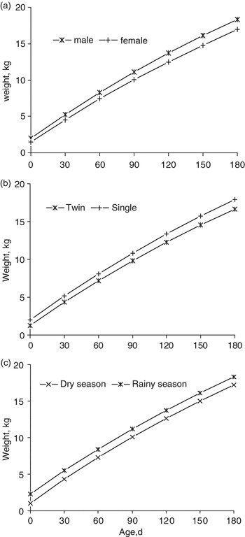
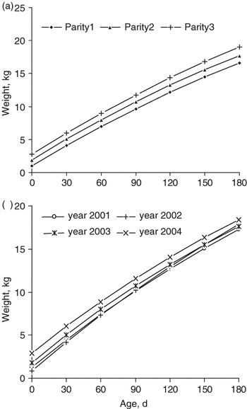
The least-squares estimate parameters A, B and k are presented in Table 3 and Table 4, with the R 2, MSE and AIC values that rank the models related to the environmental factors. All models gave higher R 2, i.e. Von Bertalanffy (0.84 to 0.87), Gompertz (0.83 to 0.87), Logistic and Brody (0.80 to 0.85), suggesting their overall good fits to the data. The Brody model was ranked the first for AIC (205.27 to 2053.1) and MSE (0.06 to 0.07) and appears to be the best fitted even though its R 2 value was little less than in Von Bertalanffy and Gompertz models. Parameters among the environmental factors in Brody model ranged from 41.8 to 51.1, 0.9360 to 0.9841 and 0.0023 to 0.0025, respectively, for A, B and k (Table 3). The shape of the growth curve showed that male (Figure 2a) and single lambs (Figure 2b) were heavier than female and twin lambs, respectively. The higher weight of male than female has been described in WAD sheep (London and Weniger, Reference London and Weniger1995; Ebangi et al., Reference Ebangi, Nwakalor, Mbah and Abba1996; Gbangboche et al., Reference Gbangboche, Youssao, Senou, Adamou-Ndiaye, Ahissou, Farnir, Michaux, Abiola and Leroy2006b) and could be attributed to the hormonal and physiological differences between sexes (Ebangi et al., Reference Ebangi, Nwakalor, Mbah and Abba1996). The superiority of single lambs over the twins was similarly reported (Armbruster et al., Reference Armbruster, Peters K and Hadji-Thomas1991a; Abassa et al., Reference Abassa, Pessinaba and Adeshola-Ishola1992; Yapi-Gnaoré et al., Reference Yapi-Gnaoré, Oya, Rege and Dagnogo1997) and in this case, the limited capacity of WAD dams to provide more nourishment for the development of multiple foetuses and more milk for new born lambs, could explain their low performance. The lambs born in rainy season were heavier and grew faster than their counterparts from the dry season (Figure 2c). Similar seasonal influences have been found in tropical area (London and Weniger, Reference London and Weniger1995; Ebangi et al., Reference Ebangi, Nwakalor, Mbah and Abba1996) and may be due to the variation of the physical environment that affect the availability and quality of forage during dry season, since the year-round grazing was the practice in Betecoucou farm. The lambs weight consistently increased with ewe parity (Figure 3a) as described in other studies (London and Weniger, Reference London and Weniger1995; Ebangi et al., Reference Ebangi, Nwakalor, Mbah and Abba1996; Yapi-Gnaoré et al., Reference Yapi-Gnaoré, Oya, Rege and Dagnogo1997). The maternal effect (i.e. nursing, the bond between ewe and lamb) is more important with elder ewes, suggesting the advantages to have high-parity ewes in the flock. Indeed, the first-parity ewes are still growing, implying the competition for nutrient with the foetuses (London and Weniger, Reference London and Weniger1995). The incidence of year (Figure 3b) was reported in previous studies (Ebangi et al., Reference Ebangi, Nwakalor, Mbah and Abba1996 and Gbangboche et al., Reference Gbangboche, Adamou-Ndiaye, Youssao, Farnir, Detilleux, Abiola and Leroy2006a and Reference Gbangboche, Youssao, Senou, Adamou-Ndiaye, Ahissou, Farnir, Michaux, Abiola and Leroy2006b) and could be due to the changes during the year, in management, herdsman’s skills and other environmental factors.
Parameters estimates ± standard error, coefficient determination (R 2), mean square error (MSE) and Akaike’s Information Criterion (AIC) of Brody and Gompertz models according to the environmental factors in West African Dwarf sheep

‡Selected model: A is the predicted asymptotic weight at maturity (kg), B is the proportional difference between A and birth weight (kg) and k is the rate of maturating.
Parameters estimates ±standard error, coefficient determination (R 2), mean squared error (MSE) and Akaike’s Information Criterion (AIC) of Logistic and Von Bertalanffy models according to the environmental factors in West African Dwarf sheep

‡Selected model: A is the predicted asymptotic weight at maturity (kg), B is the proportional difference between A and birth weight (kg) and k is the rate of maturating.
Slope of the selected Brody model according to the sex of lamb (a), type of birth (b) and season of birth (c) describing the growth in West African Dwarf sheep.

Slope of the selected Brody model according to the parity of ewe (a) and effect of year of birth (b) describing the lamb growth in West African Dwarf sheep.

Conclusion
In WAD sheep, non-linear functions described the path by which this indigenous sheep travel from birth to 180 days of age. Divergent growth response was obtained and among the four models applied (Brody, Gompertz, Logistic and Von Bertalanffy), the Brody model provides the goodness of fit for the growth curve of WAD sheep in Betecoucou breeding farm. Consequently, Brody model would serve as valuable tools for overall productivity, feeding and drug administration, since this management is commonly focused on live body weight. Otherwise, this study showed the importance to adjust the model parameter A, B and k, when environmental factors affected significantly the observed weight, in order to provide a specific slope of growth curve: in this study the shape of growth curve due to the effect of year, season of birth, sex of lamb, type or birth, parity of dam have been built. However, it cannot be assumed that the Brody model could ‘ad aeternam’ produce the goodness of fit in the Betecoucou breeding farm when the environmental conditions change. For this purpose, the model parameters need to be routinely re-adjusted, allowing even the possibility of testing all other non-linear growth models.
Appendix
Computation of Brody, Gompertz, Logistic and Von Bertalanffy models in Matlab®, 2006.
function [note1,d,note2,da]=modele(y,x)
warning off;
[n,p]=size(x);
x=[ones(n,1),x];
z=max(y);
qs=(z+1:0.1:3*z+1)';
[n1,na]=size(qs);
for i=1:n1
j=round(1+((qs(i)−z−1)/0.1));
w1=log(1−(y/qs(i)));
w2=log(log(qs(i)./y));
w3=log((qs(i)./y)−1);
w4=log(1−((y/qs(i)).^(1/3)));
u1(j,:)=mode1(w1,x);
u2(j,:)=mode1(w2,x);
u3(j,:)=mode1(w3,x);
u4(j,:)=mode1(w4,x);
end
[h1,h2]=size(u1);ua=(z+1:0.1:3*z+1)';wx=3*z+1;
l1=sortrows([ua,u1],4);la=l1(:,4);
la(1,:)=[];lb=l1(:,4);lb(h1,:)=[];q=la−lb;
b=0;
for i=1:h1−1
if q(i)<0.0001
ye(i,1)=i;
b=b+1;
end
end
ye(1:h1−1−b+5)=[];m1=l1(ye(1),:);
l2=sortrows([ua,u2],4);m2=l2(h1,:);
l3=sortrows([ua,u3],4);m3=l3(h1,:);
l4=sortrows([ua,u4],4);m4=l4(h1,:);
B1=exp(m1(1,2));B2=exp(m2(1,2));B3=exp(m3(1,2));
B4=exp(m4(1,2));
K1=−m1(1,3);K2=−m2(1,3);K3=−m3(1,3);K4=−m4(1,3);
A1=m1(1,1);A2=m2(1,1);A3=m3(1,1);A4=m4(1,1);
d1=[A1,B1,K1,m1(1,4),sqrt(m1(1,5))];d2=[A2,B2,K2,m2(1,4),sqrt(m2(1,5))];
d3=[A3,B3,K3,m3(1,4),sqrt(m3(1,5))];d4=[A4,B4,K4,m4(1,4),sqrt(m4(1,5))];
sw1=m1(1,1)*exp(m1(1,5));sw2=m2(1,1)*exp(m2(1,5));
sw3=m3(1,1)*exp(m3(1,5));sw4=m4(1,1)*exp(m4(1,5));
SCE=(n−1)*var(x(:,2));
xbar=mean(x(:,2));
ax1=1.96*sqrt(m1(1,5)*((1/n)+((xbar^2)/SCE)));
bx1=1.96*sqrt(m1(1,5)/SCE);
ax2=1.96*sqrt(m2(1,5)*((1/n)+((xbar^2)/SCE)));
bx2=1.96*sqrt(m2(1,5)/SCE);
ax3=1.96*sqrt(m3(1,5)*((1/n)+((xbar^2)/SCE)));
bx3=1.96*sqrt(m3(1,5)/SCE);
ax4=1.96*sqrt(m4(1,5)*((1/n)+((xbar^2)/SCE)));
bx4=1.96*sqrt(m4(1,5)/SCE);
Ba1=ax1;Ba2=ax2;Ba3=ax3;Ba4=ax4;
Ka1=bx1;Ka2=bx2;Ka3=bx3;Ka4=bx4;
[n1,h]=size((A1:wx)');[n2,h]=size((A2:wx)');[n3,h]=size((A3:wx)');[n4,h]=size((A4:wx)');
Aa1=std((A1:wx)')/sqrt(n1);Aa2=std((A2:wx)')/sqrt(n2);
Aa3=std((A3:wx)')/sqrt(n3);Aa4=std((A4:wx)')/sqrt(n4);
da1=[Aa1,Ba1,Ka1];da2=[Aa2,Ba2,Ka2];
da3=[Aa3,Ba3,Ka3];da4=[Aa4,Ba4,Ka4];
note1=[' A ',' B ',' k ',' Rsq ',' MSE '];
note2=[' err(A) ',' err(B) ',' err(k) '];
d=[d1;d2;d3;d4]; da=[da1;da2;da3;da4];
x1=(1:360)';wt1=A1*(1−(B1*exp(−K1*x1)));
wt2=A2*exp(−B2*exp(−K2*x1));wt3=A3./(1+B3*exp(−K3*x1));
wt4=A4.*((1−B4*exp(−K4*x1)).^3);
plot(x1,wt1,'−',x1,wt2,'−',x1,wt3,'−',x1,wt4,'−');
axis([0,180,0,30]);
legend('Brody','Gompertz','Logistic','Von Bertalanfly',2);
xlabel('Age, d)')
ylabel('Weight, kg')