

1 Introduction
Since the pioneering work of Saint-Venant (Reference Saint-Venant1871), the modelling of free-surface flows via thin-layer approaches has been the subject of countless studies in hydraulics and fluid mechanics (e.g. Whitham Reference Whitham1974; Chanson Reference Chanson2004; Kalliadasis et al. Reference Kalliadasis, Ruyer-Quil, Scheid and Velarde2012). In these models, the characteristic flow thickness  $H$ is assumed to be small compared with the characteristic flow length
 $L$, that is, the flow aspect ratio
 $\unicode[STIX]{x1D716}=H/L\ll 1$. This includes lubrication models, in which inertia terms are neglected, as well as more general shallow-water (or Saint-Venant-like) models. Lubrication models typically reduce to a single advection–diffusion equation for the evolution of flow height
 $h$ (Benney Reference Benney1966; Hunt Reference Hunt1994; Huppert Reference Huppert2006; Ancey, Cochard & Andreini Reference Ancey, Cochard and Andreini2009). Shallow-water models are generally formulated as systems of two coupled equations (in two dimensions) for flow height
 $h$ and discharge
 $q$ or depth-averaged velocity
 $\bar{u}=q/h$ (Savage & Hutter Reference Savage and Hutter1989; Ancey et al. Reference Ancey, Cochard, Rentschler and Wiederseiner2007; Iverson Reference Iverson and Fernando2013; Noble & Vila Reference Noble and Vila2013), although recently more robust three-equation models, including an additional enstrophy variable, have also been proposed (Richard, Ruyer-Quil & Vila Reference Richard, Ruyer-Quil and Vila2016). In these models, fluid rheology is accounted for through closure terms that implicitly depend on the distribution of longitudinal velocity
 $u(y)$ (with
 $y$ the cross-stream coordinate) across the flowing layer (Ng & Mei Reference Ng and Mei1994; Ruyer-Quil & Manneville Reference Ruyer-Quil and Manneville2000; Hogg & Pritchard Reference Hogg and Pritchard2004). Most of the above-mentioned references considered the case of Newtonian or generalised Newtonian (e.g. power-law) fluids, either in laminar or turbulent regimes. In this work, we focus on a more complex class of fluids, namely viscoplastic fluids characterised by a yield stress (Balmforth, Frigaard & Ovarlez Reference Balmforth, Frigaard and Ovarlez2014; Coussot Reference Coussot2014). These materials are involved in numerous industrial (Roussel & Coussot Reference Roussel and Coussot2005; Frigaard, Paso & de Souza Mendes Reference Frigaard, Paso and de Souza Mendes2017) and geophysical applications (Laigle & Coussot Reference Laigle and Coussot1997; Ancey Reference Ancey2007), for which accurate thin-layer models would be needed. Yet, as will be discussed, the viscoplastic rheology poses specific modelling issues related to the possible coexistence of unyielded (solid-like) and yielded (fluid-like) zones within the flows. Hence, attempts at developing lubrication (Huang & Garcia Reference Huang and Garcia1998; Balmforth et al. Reference Balmforth, Craster, Rust and Sassi2006; Ancey & Cochard Reference Ancey and Cochard2009; Bernabeu, Saramito & Smutek Reference Bernabeu, Saramito and Smutek2014; Liu et al. Reference Liu, Balmforth, Hormozi and Hewitt2016) or shallow-water (Coussot Reference Coussot1994; Liu & Mei Reference Liu and Mei1994; Piau Reference Piau1996; Balmforth & Liu Reference Balmforth and Liu2004) models for viscoplastic materials remained relatively rare.
Formally, thin-layer models can be derived from the primitive Cauchy equations through asymptotic expansions with respect to flow aspect ratio  $\unicode[STIX]{x1D716}$. Lubrication models proceed from a leading-order expansion (Benney Reference Benney1966; Ruyer-Quil & Manneville Reference Ruyer-Quil and Manneville1998). At the next level of approximation, derivation of consistent shallow-water models requires expansion of the velocity profile
 $u(y)$ up to at least
 $O(\unicode[STIX]{x1D716})$ terms (Ruyer-Quil & Manneville Reference Ruyer-Quil and Manneville2000; Noble & Vila Reference Noble and Vila2013). Yet, most shallow-water models used in practical applications, either for Newtonian of non-Newtonian fluids, are based on simpler, ad-hoc assumptions. Typically, closure terms are postulated empirically, or the velocity profile is assumed identical to that obtained in a steady uniform regime (see, e.g. Liu & Mei (Reference Liu and Mei1994) and Coussot (Reference Coussot1994), for viscoplastic fluids). Suchad hoc shallow-water models generally fail to predict the correct instability threshold for the flows (Ruyer-Quil & Manneville Reference Ruyer-Quil and Manneville2000; Kalliadasis et al. Reference Kalliadasis, Ruyer-Quil, Scheid and Velarde2012). From an operational point of view, these models nevertheless proved capable of producing relatively accurate predictions in terms of, for example, front propagation velocity or free-surface shape (Hogg & Pritchard Reference Hogg and Pritchard2004; Ancey, Andreini & Epely-Chauvin Reference Ancey, Andreini and Epely-Chauvin2012; Kirstetter et al. Reference Kirstetter, Hu, Delestre, Darboux, Lagrée, Popinet, Fullana and Josserand2016; Saingier, Deboeuf & Lagrée Reference Saingier, Deboeuf and Lagrée2016).
Expansions of the velocity field up to  $O(\unicode[STIX]{x1D716})$, and the use thereof in the formulation of consistent shallow-water models, have been worked out for Newtonian and power-law fluids. The handling of the two types of constitutive laws is largely similar, despite a singularity in the apparent viscosity at the free surface in the power-law case. Ruyer-Quil & Manneville (Reference Ruyer-Quil and Manneville2000) and Ruyer-Quil, Chakraborty & Dandapat (Reference Ruyer-Quil, Chakraborty and Dandapat2012) used a weighted-residual method to express deviations from the steady uniform profile in terms of polynomial test functions (see also Amaouche, Djema & Ait Aberrahmane (Reference Amaouche, Djema and Ait Aberrahmane2012)). Alternatively, Fernandez-Nieto, Noble & Vila (Reference Fernandez-Nieto, Noble and Vila2010) and Noble & Vila (Reference Noble and Vila2013) performed a formal asymptotic expansion of the primitive equations, in a regime where these equations reduce to steady uniform flow at leading order. At
 $O(\unicode[STIX]{x1D716})$, the velocity profile
 $u(y)$ then explicitly depends on flow height gradient
 $\unicode[STIX]{x2202}_{x}h$ (with
 $x$ the streamwise coordinate), and expresses as a sum of the steady uniform profile and of inertia correction terms. Shallow-water models derived from either of these two approaches were shown to correctly capture the flow instability threshold. More generally, Boutounet, Monnier & Vila (Reference Boutounet, Monnier and Vila2016) explained that a whole family of consistent shallow-water models, which are all equivalent at
 $O(\unicode[STIX]{x1D716})$, can be constructed. For practical applications, additional model selection criteria would thus be needed.
Far fewer studies focused on expansions of the velocity field in viscoplastic fluids described by Bingham or Herschel–Bulkley constitutive laws. In a steady uniform regime, the longitudinal velocity profile  $u(y)$ is composed of a yielded layer at the base, overlain by an unyielded, plug layer close to the free surface (e.g. Coussot Reference Coussot1994; Chambon, Ghemmour & Laigle Reference Chambon, Ghemmour and Laigle2009). Balmforth & Craster (Reference Balmforth and Craster1999) showed that, in thin non-uniform flows, this plug layer becomes a pseudo-plug in which the strain rate is
 $O(\unicode[STIX]{x1D716})$. These authors worked out an asymptotic expansion of the velocity profile in the pseudo-plug up to
 $O(\unicode[STIX]{x1D716})$ in the inertia-less limit. Recently, Liu, Balmforth & Hormozi (Reference Liu, Balmforth and Hormozi2019) investigated the transition between a true plug and a pseudo-plug. Balmforth & Liu (Reference Balmforth and Liu2004) used the weighted-residual approach to derive an
 $O(\unicode[STIX]{x1D716})$ velocity approximation in the sheared layer, but did not consider the correction terms in the pseudo-plug. Fernandez-Nieto et al. (Reference Fernandez-Nieto, Noble and Vila2010) applied their formal asymptotic approach to the case of a Bingham fluid and showed that, in addition to the inertia correction terms already present for fluids without a yield stress, the
 $O(\unicode[STIX]{x1D716})$ velocity approximation also involves correction terms arising from the existence of
 $O(1)$ normal stresses in the pseudo-plug. These latter authors also proposed the (to date) only consistent shallow-water model for a viscoplastic rheology. However, variations of pseudo-plug thickness along the flow are not considered in this model. Lubrication-like models, in contrast, predict a dependence of pseudo-plug thickness on flow height gradient
 $\unicode[STIX]{x2202}_{x}h$ (Balmforth & Craster Reference Balmforth and Craster1999; Ancey & Cochard Reference Ancey and Cochard2009; Freydier, Chambon & Naaim Reference Freydier, Chambon and Naaim2017), and one would like
 $O(\unicode[STIX]{x1D716})$ models to recover this feature when inertia terms are neglected.
In this context, the objectives of the present study are twofold. First, expanding on the approach of Fernandez-Nieto et al. (Reference Fernandez-Nieto, Noble and Vila2010), we derive a complete  $O(\unicode[STIX]{x1D716})$ expansion of longitudinal velocity profile
 $u(y)$ in a Herschel–Bulkley thin free-surface flow, accounting for possible variations in pseudo-plug thickness. As will be shown, the expression obtained depends on gradients of both flow height and pseudo-plug thickness. The prospect of formulating consistent shallow-water models based on this asymptotic expansion of velocity is left for future work. Instead, we assess the differences between the leading-order and
 $O(\unicode[STIX]{x1D716})$ velocity approximations in the specific case of travelling-wave solutions, for which the evolution of free surface can be computed without additional developments. The second objective is then to compare these asymptotic velocity predictions with high-resolution experimental data recently obtained by our group (Freydier et al. Reference Freydier, Chambon and Naaim2017). Our previous work showed in particular that, in viscoplastic free-surface surges, longitudinal velocity profiles measured close to the tip clearly diverge from the predictions of a leading-order lubrication model. Our goal here is therefore to investigate whether an
 $O(\unicode[STIX]{x1D716})$ approximation provides a better match to the data.
Formal asymptotic expansion of the velocity field is derived in § 2. Section 3 examines the influence of the different correction terms involved in the  $O(\unicode[STIX]{x1D716})$ approximation, as a function of the relevant non-dimensional parameters. Experimental results are briefly recalled, and compared with the theoretical predictions, in § 4. Finally, §§ 5 and 6 discuss and summarise the main outcomes of the study. Additional results obtained with Newtonian fluids are presented in appendix B.
2 Thin-layer asymptotic expansion
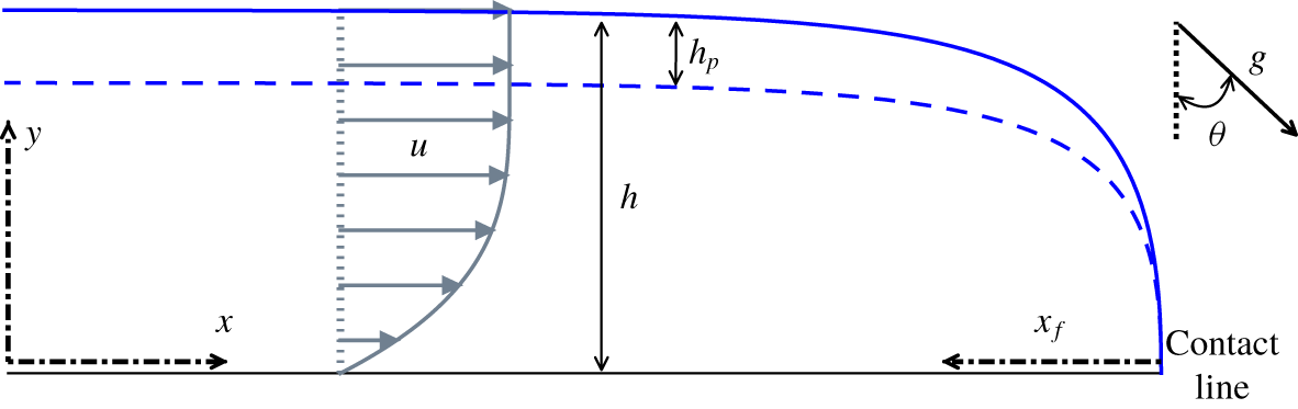
Let us consider a free-surface viscoplastic surge propagating down an inclined plane forming an angle  $\unicode[STIX]{x1D703}$ to the horizontal (figure 1). The flow is driven by gravity
 $\boldsymbol{g}$. The
 $x$-axis (hereafter called longitudinal) coincides with the base plane in the streamwise direction, while the
 $y$-axis (hereafter called vertical) is orthogonal to the bed, pointing upwards. Flow is assumed to be two dimensional, that is, independent of the spanwise direction. Fluid density is denoted by
 $\unicode[STIX]{x1D70C}$, local flow thickness by
 $h(x,t)$ and fluid velocity by
 $\boldsymbol{u}(x,y,t)$.
Free-surface viscoplastic surge down an incline: flow configuration considered in this study (see notation in the text). The dashed line represents the fake yield surface.

The viscoplastic fluid is assumed to obey the Herschel–Bulkley constitutive law:
 $$\begin{eqnarray}\left.\begin{array}{@{}c@{}}\displaystyle \unicode[STIX]{x1D70F}_{ij}=\left({\displaystyle \frac{\unicode[STIX]{x1D70F}_{c}}{|\dot{\unicode[STIX]{x1D6FE}}|}}+K|\dot{\unicode[STIX]{x1D6FE}}|^{n-1}\right)\dot{\unicode[STIX]{x1D6FE}}_{ij}\quad \text{if }|\unicode[STIX]{x1D70F}|>\unicode[STIX]{x1D70F}_{c},\\ \dot{\unicode[STIX]{x1D6FE}}_{ij}=0\quad \text{if }|\unicode[STIX]{x1D70F}|\leqslant \unicode[STIX]{x1D70F}_{c},\end{array}\right\}\end{eqnarray}$$
where  $\unicode[STIX]{x1D70F}_{ij}=\unicode[STIX]{x1D70E}_{ij}+p\unicode[STIX]{x1D6FF}_{ij}$ is the extra-stress tensor (with
 $\unicode[STIX]{x1D70E}_{ij}$ the total stress and
 $p$ the pressure) and
 $\dot{\unicode[STIX]{x1D6FE}}_{ij}=\unicode[STIX]{x2202}_{j}u_{i}+\unicode[STIX]{x2202}_{i}u_{j}$ is the strain-rate tensor. The tensorial norm is defined as
 $|\unicode[STIX]{x1D64F}|=(0.5\unicode[STIX]{x1D61B}_{ij}\unicode[STIX]{x1D61B}_{ij})^{0.5}$ for any second-order tensor
 $\unicode[STIX]{x1D64F}$. Rheological parameters
 $\unicode[STIX]{x1D70F}_{c}$,
 $K$ and
 $n$ correspond to the yield stress, the consistency and the power index of the material, respectively. We assume
 $n>0$, and shall consider more specifically the two cases
 $n=1$ (Bingham fluid) and
 $n\approx 0.4$ (shear-thinning value representative of most real viscoplastic fluids). In the following, for
 $|\unicode[STIX]{x1D70F}|>\unicode[STIX]{x1D70F}_{c}$, we split the extra-stress tensor into its viscous and plastic contributions:
 $\unicode[STIX]{x1D70F}_{ij}=\unicode[STIX]{x1D70F}_{ij}^{v}+\unicode[STIX]{x1D70F}_{ij}^{p}$, with
 $\unicode[STIX]{x1D70F}_{ij}^{v}=K|\dot{\unicode[STIX]{x1D6FE}}|^{n-1}\dot{\unicode[STIX]{x1D6FE}}_{ij}$ and
 $\unicode[STIX]{x1D70F}_{ij}^{p}=(\unicode[STIX]{x1D70F}_{c}/|\dot{\unicode[STIX]{x1D6FE}}|)\dot{\unicode[STIX]{x1D6FE}}_{ij}$.
2.1 Primitive equations
Let  $u=u_{x}$ and
 $v=u_{y}$ denote the longitudinal and vertical velocity components, respectively. The primitive equations governing free-surface flows of viscoplastic fluids are derived in numerous previous references (e.g. Piau Reference Piau1996; Ancey & Cochard Reference Ancey and Cochard2009; Fernandez-Nieto et al. Reference Fernandez-Nieto, Noble and Vila2010). Here, we recall them directly in dimensionless form. Hence, let us define the Reynolds, Froude and Bingham numbers as
 $$\begin{eqnarray}Re=\frac{\unicode[STIX]{x1D70C}U^{2-n}H^{n}}{K},\quad Fr=\frac{U}{\sqrt{gH\cos \unicode[STIX]{x1D703}}},\quad Bi=\frac{\unicode[STIX]{x1D70F}_{c}}{K}\left(\frac{H}{U}\right)^{n},\end{eqnarray}$$
where  $H$,
 $L$ and
 $U$ represent a characteristic thickness, a characteristic length and a characteristic longitudinal velocity of the flow, respectively. Pressure
 $p$ is scaled by
 $\unicode[STIX]{x1D70C}gH\cos \unicode[STIX]{x1D703}$ and shear rate
 $|\dot{\unicode[STIX]{x1D6FE}}|$ is scaled by
 $U/H$. We choose to scale the viscous contribution to stresses by
 $K(U/H)^{n}$, and the plastic contribution by
 $\unicode[STIX]{x1D70F}_{c}$. Lastly, the stress norm
 $|\unicode[STIX]{x1D70F}|$ is scaled by
 $K(U/H)^{n}$, such that the dimensionless yield condition can be written
 $|\unicode[STIX]{x1D70F}|=Bi$.
Dimensionless mass and momentum conservation equations then read
 $$\begin{eqnarray}\displaystyle & \displaystyle \unicode[STIX]{x2202}_{x}u+\unicode[STIX]{x2202}_{y}v=0, & \displaystyle\end{eqnarray}$$
 $$\begin{eqnarray}\displaystyle & \displaystyle \unicode[STIX]{x1D716}Re\;(\unicode[STIX]{x2202}_{t}u+u\unicode[STIX]{x2202}_{x}u+v\unicode[STIX]{x2202}_{y}u)=-\frac{\unicode[STIX]{x1D716}Re}{Fr^{2}}\unicode[STIX]{x2202}_{x}p+\unicode[STIX]{x1D706}+\unicode[STIX]{x2202}_{y}\unicode[STIX]{x1D70F}_{xy}^{v}+Bi\unicode[STIX]{x2202}_{y}\unicode[STIX]{x1D70F}_{xy}^{p}+\unicode[STIX]{x1D716}(\unicode[STIX]{x2202}_{x}\unicode[STIX]{x1D70F}_{xx}^{v}+Bi\unicode[STIX]{x2202}_{x}\unicode[STIX]{x1D70F}_{xx}^{p}),\qquad & \displaystyle\end{eqnarray}$$
 $$\begin{eqnarray}\displaystyle \unicode[STIX]{x1D716}^{3}Re\;(\unicode[STIX]{x2202}_{t}v+u\unicode[STIX]{x2202}_{x}v+v\unicode[STIX]{x2202}_{y}v) & = & \displaystyle -\frac{\unicode[STIX]{x1D716}Re}{Fr^{2}}(1+\unicode[STIX]{x2202}_{y}p)\nonumber\\ \displaystyle & & \displaystyle +\,\unicode[STIX]{x1D716}^{2}(\unicode[STIX]{x2202}_{x}\unicode[STIX]{x1D70F}_{xy}^{v}+Bi\unicode[STIX]{x2202}_{x}\unicode[STIX]{x1D70F}_{xy}^{p})+\unicode[STIX]{x1D716}(\unicode[STIX]{x2202}_{y}\unicode[STIX]{x1D70F}_{yy}^{v}+Bi\unicode[STIX]{x2202}_{y}\unicode[STIX]{x1D70F}_{yy}^{p}),\end{eqnarray}$$
where we recall that  $\unicode[STIX]{x1D716}=H/L$ is flow aspect ratio, and the driving parameter
 $\unicode[STIX]{x1D706}$ is given by
 $$\begin{eqnarray}\unicode[STIX]{x1D706}=\frac{\unicode[STIX]{x1D70C}gH^{n+1}\sin \unicode[STIX]{x1D703}}{KU^{n}}=\frac{Re}{Fr^{2}}\tan \unicode[STIX]{x1D703}.\end{eqnarray}$$
The dimensionless expressions of viscous and plastic stresses, for  $|\unicode[STIX]{x1D70F}|>Bi$, can be written
 $$\begin{eqnarray}\displaystyle & \displaystyle \unicode[STIX]{x1D70F}_{xx}^{v}=-\unicode[STIX]{x1D70F}_{yy}^{v}=2\unicode[STIX]{x1D716}|\dot{\unicode[STIX]{x1D6FE}}|^{n-1}\unicode[STIX]{x2202}_{x}u, & \displaystyle\end{eqnarray}$$
 $$\begin{eqnarray}\displaystyle & \displaystyle \unicode[STIX]{x1D70F}_{xy}^{v}=|\dot{\unicode[STIX]{x1D6FE}}|^{n-1}(\unicode[STIX]{x2202}_{y}u+\unicode[STIX]{x1D716}^{2}\unicode[STIX]{x2202}_{x}v) & \displaystyle\end{eqnarray}$$
and
 $$\begin{eqnarray}\displaystyle & \displaystyle \unicode[STIX]{x1D70F}_{xx}^{p}=-\unicode[STIX]{x1D70F}_{yy}^{p}=\frac{2\unicode[STIX]{x1D716}}{|\dot{\unicode[STIX]{x1D6FE}}|}\unicode[STIX]{x2202}_{x}u, & \displaystyle\end{eqnarray}$$
 $$\begin{eqnarray}\displaystyle & \displaystyle \unicode[STIX]{x1D70F}_{xy}^{p}=\frac{1}{|\dot{\unicode[STIX]{x1D6FE}}|}(\unicode[STIX]{x2202}_{y}u+\unicode[STIX]{x1D716}^{2}\unicode[STIX]{x2202}_{x}v). & \displaystyle\end{eqnarray}$$
The equality  $\unicode[STIX]{x1D70F}_{xx}=-\unicode[STIX]{x1D70F}_{yy}$ ensues from mass conservation (2.3). Lastly, the dimensionless stress norm can be expressed as
 $$\begin{eqnarray}|\unicode[STIX]{x1D70F}|=\sqrt{(\unicode[STIX]{x1D70F}_{xy}^{v}+Bi\unicode[STIX]{x1D70F}_{xy}^{p})^{2}+(\unicode[STIX]{x1D716}\unicode[STIX]{x1D70F}_{xx}^{v}+Bi\unicode[STIX]{x1D70F}_{xx}^{p})^{2}},\end{eqnarray}$$
and the dimensionless shear rate can be expressed as
 $$\begin{eqnarray}|\dot{\unicode[STIX]{x1D6FE}}|=\sqrt{(\unicode[STIX]{x2202}_{y}u+\unicode[STIX]{x1D716}^{2}\unicode[STIX]{x2202}_{x}v)^{2}+4\unicode[STIX]{x1D716}^{2}(\unicode[STIX]{x2202}_{x}u)^{2}}.\end{eqnarray}$$
The above balance equations are to be complemented with appropriate boundary conditions. At the base, we consider a classical no-penetration and no-slip condition:  $u_{|y=0}=v_{|y=0}=0$. At the free surface, the influence of surface tension is neglected and a stress-free condition is assumed:
 $(\unicode[STIX]{x1D749}-p\unicode[STIX]{x1D644})_{|y=h}\boldsymbol{\cdot }\boldsymbol{n}=0$, with
 $\boldsymbol{n}=(-\unicode[STIX]{x2202}_{x}h,1)$ and
 $\unicode[STIX]{x1D644}$ the identity tensor. Rearranging terms, we obtain
 $$\begin{eqnarray}\displaystyle & \displaystyle (\unicode[STIX]{x1D70F}_{xy}^{v}+Bi\unicode[STIX]{x1D70F}_{xy}^{p})_{|y=h}=\frac{2\unicode[STIX]{x1D716}\unicode[STIX]{x2202}_{x}h}{1-\unicode[STIX]{x1D716}^{2}(\unicode[STIX]{x2202}_{x}h)^{2}}(\unicode[STIX]{x1D716}\unicode[STIX]{x1D70F}_{xx}^{v}+Bi\unicode[STIX]{x1D70F}_{xx}^{p})_{|y=h}, & \displaystyle\end{eqnarray}$$
 $$\begin{eqnarray}\displaystyle & \displaystyle p_{|y=h}=-\frac{Fr^{2}}{Re}\frac{1+\unicode[STIX]{x1D716}^{2}(\unicode[STIX]{x2202}_{x}h)^{2}}{1-\unicode[STIX]{x1D716}^{2}(\unicode[STIX]{x2202}_{x}h)^{2}}(\unicode[STIX]{x1D716}\unicode[STIX]{x1D70F}_{xx}^{v}+Bi\unicode[STIX]{x1D70F}_{xx}^{p})_{|y=h}. & \displaystyle\end{eqnarray}$$
Finally, the following kinematic condition holds at the free surface:
 $$\begin{eqnarray}\unicode[STIX]{x2202}_{t}h+u_{|y=h}\unicode[STIX]{x2202}_{x}h=v_{|y=h}.\end{eqnarray}$$
For completeness, we also recall the depth-averaged mass-conservation equation
 $$\begin{eqnarray}\unicode[STIX]{x2202}_{t}h+\unicode[STIX]{x2202}_{x}q=0,\end{eqnarray}$$
where  $q=\int _{0}^{h}u\,\text{d}y$ is flow discharge. This equation is readily obtained from integration of local mass conservation (2.3) and boundary conditions.
2.2 Flow regime
Following the approach of Fernandez-Nieto et al. (Reference Fernandez-Nieto, Noble and Vila2010), we aim to derive approximations of the velocity field in the flow through formal asymptotic expansions of the previous primitive equations with respect to  $\unicode[STIX]{x1D716}$. The following assumptions are introduced: (i)
 $\unicode[STIX]{x1D716}\ll 1$ (thin-layer approximation); (ii) the factor
 $\unicode[STIX]{x1D716}Re$ in front of inertia terms in (2.4) is considered
 $O(\unicode[STIX]{x1D716})$; (iii) as the study concerns flows in which plastic effects are significant, the Bingham number
 $Bi$ is considered
 $O(1)$; and (iv) finally, the factor
 $\unicode[STIX]{x1D716}Re/Fr^{2}$ in front of pressure gradient terms in (2.4)–(2.5) is also considered
 $O(1)$. This latter assumption constitutes the main difference from the work of Fernandez-Nieto et al. (Reference Fernandez-Nieto, Noble and Vila2010), in which
 $\unicode[STIX]{x1D716}Re/Fr^{2}$ was considered
 $O(\unicode[STIX]{x1D716})$. Accordingly, the flow regime investigated in the present study corresponds, at leading order, to a balance between pressure gradient, gravity and shear stress effects, as in classical lubrication models. Note that the assumption
 $\unicode[STIX]{x1D716}Re/Fr^{2}=O(1)$ implicitly requires the slope angle
 $\unicode[STIX]{x1D703}$ to be small, so that
 $\unicode[STIX]{x1D706}=\unicode[STIX]{x1D716}Re/Fr^{2}(\tan \unicode[STIX]{x1D703}/\unicode[STIX]{x1D716})$ can also be
 $O(1)$.
We assume the existence of regular expansions of the form:  $f=f^{(0)}+\unicode[STIX]{x1D716}f^{(1)}+\cdots \,$, for all variables of interest, namely longitudinal and vertical velocities
 $u$ and
 $v$, pressure
 $p$ and stress components
 $\unicode[STIX]{x1D70F}_{ij}$. As will be shown, these expansions can effectively be formally worked out up to
 $O(\unicode[STIX]{x1D716})$. Let us note, however, that the residues, whose complete evaluation lies outside the scope of this article, are not necessarily
 $O(\unicode[STIX]{x1D716}^{2})$ and may involve terms depending on non-integer powers
 $\unicode[STIX]{x1D716}^{a}$ (with
 $a>1$) (Fernandez-Nieto et al. Reference Fernandez-Nieto, Noble and Vila2010).
2.3 Leading-order expansion
At  $O(1)$ with respect to
 $\unicode[STIX]{x1D716}$, integration of (2.4)–(2.5) leads to linear profiles for the shear stress and pressure:
 $$\begin{eqnarray}\displaystyle & \displaystyle \unicode[STIX]{x1D70F}_{xy}^{v,(0)}+Bi\unicode[STIX]{x1D70F}_{xy}^{p,(0)}=\unicode[STIX]{x1D6EC}(x,t)\;(h-y), & \displaystyle\end{eqnarray}$$
 $$\begin{eqnarray}\displaystyle & \displaystyle p^{(0)}=(h-y), & \displaystyle\end{eqnarray}$$
where we introduced
 $$\begin{eqnarray}\unicode[STIX]{x1D6EC}(x,t)=\unicode[STIX]{x1D706}-\frac{\unicode[STIX]{x1D716}Re}{Fr^{2}}\unicode[STIX]{x2202}_{x}h=\unicode[STIX]{x1D706}\;(1-\unicode[STIX]{x1D716}\cot \unicode[STIX]{x1D703}\unicode[STIX]{x2202}_{x}h).\end{eqnarray}$$
Moreover, the Herschel–Bulkley law, for  $|\unicode[STIX]{x1D70F}|>Bi$, reduces to
 $$\begin{eqnarray}\unicode[STIX]{x1D70F}_{xy}^{v,(0)}+Bi\unicode[STIX]{x1D70F}_{xy}^{p,(0)}=\operatorname{sgn}(\unicode[STIX]{x2202}_{y}u^{(0)})(\unicode[STIX]{x2202}_{y}u^{(0)})^{n}+Bi\end{eqnarray}$$
and  $\unicode[STIX]{x1D70F}_{xx}^{p,(0)}=\unicode[STIX]{x1D70F}_{xx}^{v,(0)}=0$. From these leading-order expressions, we expect the existence of an unsheared layer, in which
 $|\dot{\unicode[STIX]{x1D6FE}}|^{(0)}=|\unicode[STIX]{x2202}_{y}u^{(0)}|=0$, for
 $y\geqslant h-h_{p}$. The thickness of this layer is given by
 $$\begin{eqnarray}h_{p}=\frac{Bi}{\unicode[STIX]{x1D6EC}}.\end{eqnarray}$$
We may assume, without loss of generality, that  $\unicode[STIX]{x2202}_{y}u^{(0)}\geqslant 0$. Integration of (2.17) then leads to the classical lubrication velocity profile
 $$\begin{eqnarray}u^{(0)}=\left\{\begin{array}{@{}ll@{}}u_{pl}^{(0)}(1-\unicode[STIX]{x1D701}^{(n+1)/n}),\quad & \text{if }y<h-h_{p},\\ u_{pl}^{(0)},\quad & \text{if }y\geqslant h-h_{p},\end{array}\right.\end{eqnarray}$$
where  $\unicode[STIX]{x1D701}=1-y/(h-h_{p})$ is a reduced vertical coordinate, and
 $$\begin{eqnarray}u_{pl}^{(0)}=\frac{n}{n+1}\unicode[STIX]{x1D6EC}^{1/n}(h-h_{p})^{(n+1)/n}.\end{eqnarray}$$
It should be emphasised that  $h_{p}$,
 $\unicode[STIX]{x1D6EC}$ and, thus,
 $u_{pl}^{(0)}$ are all functions of
 $x$ and
 $t$ through the term
 $\unicode[STIX]{x2202}_{x}h$ in (2.19). If
 $\unicode[STIX]{x1D716}Re/Fr^{2}=0$, expressions (2.22)–(2.23) reduce to the velocity profile obtained in a steady uniform regime, with a constant plug thickness
 $h_{p}=Bi/\unicode[STIX]{x1D706}$ (e.g. Chambon, Ghemmour & Naaim Reference Chambon, Ghemmour and Naaim2014).
The leading-order approximation of discharge  $q$ immediately proceeds from (2.22):
 $$\begin{eqnarray}q^{(0)}=\frac{n}{2n+1}\unicode[STIX]{x1D6EC}^{1/n}(h-h_{p})^{(n+1)/n}\left(h+\frac{n}{n+1}h_{p}\right).\end{eqnarray}$$
In the following (see § 2.5), leading-order expressions of vertical velocity  $v^{(0)}$ and derivatives
 $\unicode[STIX]{x2202}_{x,t}u^{(0)}$ will also be required. These quantities are easily derived from (2.22) and mass conservation (2.3), and we shall not provide the full expressions in this article (see Freydier et al. (Reference Freydier, Chambon and Naaim2017), for expression of
 $v^{(0)}$). Let us nevertheless mention that, compared with the developments of Fernandez-Nieto et al. (Reference Fernandez-Nieto, Noble and Vila2010), additional complexities arise here from terms proportional to the derivatives
 $\unicode[STIX]{x2202}_{x,t}h_{p}$ and
 $\unicode[STIX]{x2202}_{x,t}\unicode[STIX]{x1D6EC}$. These derivatives can be interchanged through the following relation:
 $$\begin{eqnarray}\unicode[STIX]{x2202}_{x,t}h_{p}=-\frac{h_{p}}{\unicode[STIX]{x1D6EC}}\unicode[STIX]{x2202}_{x,t}\unicode[STIX]{x1D6EC}.\end{eqnarray}$$
2.4 Pseudo-plug
The dependence upon  $x$ of
 $u_{pl}^{(0)}$ appears incompatible with a strictly zero shear rate
 $|\dot{\unicode[STIX]{x1D6FE}}|$ for
 $y\geqslant h-h_{p}$, as would be expected in a ‘true’ unyielded plug. As observed by Balmforth & Craster (Reference Balmforth and Craster1999), this apparent paradox is overcome by noting that, because
 $\unicode[STIX]{x2202}_{y}u^{(0)}=0$ in this layer, the expansion of longitudinal velocity takes the form
 $u=u_{pl}^{(0)}(x,t)+\unicode[STIX]{x1D716}u_{pl}^{(1)}(x,y,t)+\cdots \,$. Accordingly, the leading-order expression of shear rate
 $|\dot{\unicode[STIX]{x1D6FE}}|$ becomes
 $$\begin{eqnarray}|\dot{\unicode[STIX]{x1D6FE}}|=\unicode[STIX]{x1D716}\sqrt{(\unicode[STIX]{x2202}_{y}u_{pl}^{(1)})^{2}+4(\unicode[STIX]{x2202}_{x}u_{pl}^{(0)})^{2}}+\cdots \,,\end{eqnarray}$$
such that the expansion of the Herschel–Bulkley law also needs to be revisited. In particular, unlike for  $y<h-h_{p}$, the plastic normal stress
 $\unicode[STIX]{x1D70F}_{xx}^{p}$ involves an
 $O(1)$ contribution
 $$\begin{eqnarray}\unicode[STIX]{x1D70F}_{xx}^{p,(0)}=\frac{2\unicode[STIX]{x2202}_{x}u_{pl}^{(0)}}{\sqrt{(\unicode[STIX]{x2202}_{y}u_{pl}^{(1)})^{2}+4(\unicode[STIX]{x2202}_{x}u_{pl}^{(0)})^{2}}}\end{eqnarray}$$
and the leading-order expression of shear stress becomes
 $$\begin{eqnarray}\unicode[STIX]{x1D70F}_{xy}^{v,(0)}+Bi\unicode[STIX]{x1D70F}_{xy}^{p,(0)}=Bi\unicode[STIX]{x1D70F}_{xy}^{p,(0)}=Bi\frac{\unicode[STIX]{x2202}_{y}u_{pl}^{(1)}}{\sqrt{(\unicode[STIX]{x2202}_{y}u_{pl}^{(1)})^{2}+4(\unicode[STIX]{x2202}_{x}u_{pl}^{(0)})^{2}}}.\end{eqnarray}$$
It ensues that the stress norm can be expressed as
 $$\begin{eqnarray}|\unicode[STIX]{x1D70F}|=Bi+O(\unicode[STIX]{x1D716}^{n}),\end{eqnarray}$$
where the residue  $O(\unicode[STIX]{x1D716}^{n})$ is necessarily positive. Hence, plastic normal stresses actually make up for the small values of shear stress, and are sufficient for the yield criterion to be slightly exceeded. The unsheared layer predicted by the leading-order velocity expansion should thus rather be considered as a pseudo-plug, in which the shear rate is
 $O(\unicode[STIX]{x1D716})$. Accordingly, the interface at
 $y=h-h_{p}$ should be regarded as a fake yield surface.
Combining (2.28) and (2.17) leads to
 $$\begin{eqnarray}\unicode[STIX]{x2202}_{y}u_{pl}^{(1)}=\frac{2(h-y)/h_{p}}{\sqrt{1-((h-y)/h_{p})^{2}}}|\unicode[STIX]{x2202}_{x}u_{pl}^{(0)}|,\end{eqnarray}$$
where (2.21) was used to express pseudo-plug thickness  $h_{p}$. From (2.26), the shear rate in the pseudo-plug can then be expressed as
 $$\begin{eqnarray}|\dot{\unicode[STIX]{x1D6FE}}|=\unicode[STIX]{x1D716}\frac{2}{\sqrt{1-((h-y)/h_{p})^{2}}}|\unicode[STIX]{x2202}_{x}u_{pl}^{(0)}|+\cdots \,.\end{eqnarray}$$
Finally, leading-order plastic normal stress in the pseudo-plug can be written
 $$\begin{eqnarray}\unicode[STIX]{x1D70F}_{xx}^{p,(0)}=\sqrt{1-\left(\frac{h-y}{h_{p}}\right)^{2}}\operatorname{sgn}(\unicode[STIX]{x2202}_{x}u_{pl}^{(0)}).\end{eqnarray}$$
Note that this expression for  $\unicode[STIX]{x1D70F}_{xx}^{p,(0)}$ requires
 $\unicode[STIX]{x2202}_{x}u_{pl}^{(0)}\neq 0$. If
 $\unicode[STIX]{x2202}_{x}u_{pl}^{(0)}=0$, we are either in a true plug (
 $|\dot{\unicode[STIX]{x1D6FE}}|=0$), or the shear rate in the pseudo-plug vanishes at
 $O(\unicode[STIX]{x1D716})$ and a leading term of higher order needs to be considered in the expansion of
 $|\dot{\unicode[STIX]{x1D6FE}}|$ (Fernandez-Nieto et al. Reference Fernandez-Nieto, Noble and Vila2010). This latter case will not be considered in this study.
2.5  $O(\unicode[STIX]{x1D716})$ expansion

At  $O(\unicode[STIX]{x1D716})$, velocity expansions in the pseudo-plug (
 $y\geqslant h-h_{p}$) and in the sheared layer (
 $y<h-h_{p}$) need to be treated separately.
2.5.1 In the pseudo-plug ($y\geqslant h-h_{p}$)

As seen in § 2.4, the  $O(\unicode[STIX]{x1D716})$ velocity correction in the pseudo-plug derives directly from the leading-order approximation of shear stress. Integrating (2.30) between
 $y=h-h_{p}$ and
 $y>h-h_{p}$, and accounting for the expression of
 $\unicode[STIX]{x2202}_{x}u_{pl}^{(0)}$, leads to
 $$\begin{eqnarray}u_{pl}^{(1)}=Bi\;{\mathcal{U}}_{Npl}(x,y,t)+u_{+}(x,t),\end{eqnarray}$$
where
 $$\begin{eqnarray}\displaystyle {\mathcal{U}}_{Npl}(x,y,t) & = & \displaystyle 2\unicode[STIX]{x1D6EC}^{(1-n)/n}(h-h_{p})^{1/n}\sqrt{1-\left(\frac{h-y}{h_{p}}\right)^{2}}\nonumber\\ \displaystyle & & \displaystyle \times \,\left[\unicode[STIX]{x2202}_{x}h+\frac{1}{n+1}(h+nh_{p})\frac{\unicode[STIX]{x2202}_{x}\unicode[STIX]{x1D6EC}}{\unicode[STIX]{x1D6EC}}\right]\operatorname{sgn}(\unicode[STIX]{x2202}_{x}u_{pl}^{(0)})\end{eqnarray}$$
and  $u_{+}(x,t)$ is a matching term (see § 2.5.3).
2.5.2 In the sheared layer ($y<h-h_{p}$)

Expansion at  $O(\unicode[STIX]{x1D716})$ of momentum balance equations (2.4) and (2.5) leads to
 $$\begin{eqnarray}\displaystyle \unicode[STIX]{x2202}_{y}(\unicode[STIX]{x1D70F}_{xy}^{v,(1)}+Bi\unicode[STIX]{x1D70F}_{xy}^{p,(1)}) & = & \displaystyle \frac{\unicode[STIX]{x1D716}Re}{Fr^{2}}\unicode[STIX]{x2202}_{x}p^{(1)}-Bi\unicode[STIX]{x2202}_{x}\unicode[STIX]{x1D70F}_{xx}^{p,(0)}\nonumber\\ \displaystyle & & \displaystyle +\,Re\;(\unicode[STIX]{x2202}_{t}u^{(0)}+u^{(0)}\unicode[STIX]{x2202}_{x}u^{(0)}+v^{(0)}\unicode[STIX]{x2202}_{y}u^{(0)}),\end{eqnarray}$$
 $$\begin{eqnarray}\frac{\unicode[STIX]{x1D716}Re}{Fr^{2}}\unicode[STIX]{x2202}_{y}p^{(1)}=-Bi\unicode[STIX]{x2202}_{y}\unicode[STIX]{x1D70F}_{xx}^{p,(0)}.\end{eqnarray}$$
Accounting for boundary conditions at the free surface, integration of (2.36) provides
 $$\begin{eqnarray}\frac{\unicode[STIX]{x1D716}Re}{Fr^{2}}p^{(1)}=-Bi\unicode[STIX]{x1D70F}_{xx}^{p,(0)},\end{eqnarray}$$
for all values of  $y$. Accordingly,
 $p^{(1)}=0$ for
 $y<h-h_{p}$. Equation (2.37) also shows that the two terms
 $(\unicode[STIX]{x1D716}Re/Fr^{2})\unicode[STIX]{x2202}_{x}p^{(1)}$ and
 $-Bi\unicode[STIX]{x2202}_{x}\unicode[STIX]{x1D70F}_{xx}^{p,(0)}$, involved in (2.35), are equal everywhere in the flow. Integration of (2.35) between
 $y<h-h_{p}$ and
 $y=h$ then leads to the expression of the
 $O(\unicode[STIX]{x1D716})$ shear-stress correction in the sheared layer:
 $$\begin{eqnarray}\unicode[STIX]{x1D70F}_{xy}^{v,(1)}+Bi\unicode[STIX]{x1D70F}_{xy}^{p,(1)}=-Bi\frac{\unicode[STIX]{x03C0}}{2}\frac{h_{p}}{\unicode[STIX]{x1D6EC}}\operatorname{sgn}(\unicode[STIX]{x2202}_{x}u_{pl}^{(0)})\unicode[STIX]{x2202}_{x}\unicode[STIX]{x1D6EC}+Re\;{\mathcal{I}}(x,y,t),\end{eqnarray}$$
with
 $$\begin{eqnarray}{\mathcal{I}}(x,y,t)=-\int _{y}^{h}(\unicode[STIX]{x2202}_{t}u^{(0)}+u^{(0)}\unicode[STIX]{x2202}_{x}u^{(0)}+v^{(0)}\unicode[STIX]{x2202}_{y}u^{(0)})\,\text{d}y.\end{eqnarray}$$
The first term on the right-hand side of (2.38) arises from the calculation of
 $$\begin{eqnarray}2Bi\int _{h-h_{p}}^{h}\unicode[STIX]{x2202}_{x}\unicode[STIX]{x1D70F}_{xx}^{p,(0)}\,\text{d}y+(\unicode[STIX]{x1D70F}_{xy}^{v,(1)}+Bi\unicode[STIX]{x1D70F}_{xy}^{p,(1)})_{|y=h},\end{eqnarray}$$
where the integral of  $\unicode[STIX]{x2202}_{x}\unicode[STIX]{x1D70F}_{xx}^{p,(0)}$ is restricted to the range
 $[h-h_{p},h]$, because
 $\unicode[STIX]{x1D70F}_{xx}^{p,(0)}=0$ for
 $y<h-h_{p}$, and is evaluated from (2.32).
Expansion of the Herschel–Bulkley law at  $O(\unicode[STIX]{x1D716})$ for
 $y<h-h_{p}$ can be written as
 $$\begin{eqnarray}\unicode[STIX]{x1D70F}_{xy}^{v,(0)}+Bi\unicode[STIX]{x1D70F}_{xy}^{p,(0)}+\unicode[STIX]{x1D716}(\unicode[STIX]{x1D70F}_{xy}^{v,(1)}+Bi\unicode[STIX]{x1D70F}_{xy}^{p,(1)})=(\unicode[STIX]{x2202}_{y}u^{(0)}+\unicode[STIX]{x1D716}\unicode[STIX]{x2202}_{y}u^{(1)})^{n}+Bi\end{eqnarray}$$
considering that  $|\dot{\unicode[STIX]{x1D6FE}}|^{(0)}+\unicode[STIX]{x1D716}|\dot{\unicode[STIX]{x1D6FE}}|^{(1)}=|\unicode[STIX]{x2202}_{y}u^{(0)}+\unicode[STIX]{x1D716}\unicode[STIX]{x2202}_{y}u^{(1)}|$. We assumed, again, that
 $\unicode[STIX]{x2202}_{y}u^{(0)}+\unicode[STIX]{x1D716}\unicode[STIX]{x2202}_{y}u^{(1)}\geqslant 0$. A Taylor expansion then leads to
 $$\begin{eqnarray}\unicode[STIX]{x2202}_{y}u^{(1)}=\frac{1}{n}(\unicode[STIX]{x2202}_{y}u^{(0)})^{1-n}(\unicode[STIX]{x1D70F}_{xy}^{v,(1)}+Bi\unicode[STIX]{x1D70F}_{xy}^{p,(1)}).\end{eqnarray}$$
Finally, inserting (2.38) into (2.42) and further integrating provides the  $O(\unicode[STIX]{x1D716})$ longitudinal-velocity correction for
 $y<h-h_{p}$:
 $$\begin{eqnarray}u^{(1)}=Bi\;{\mathcal{U}}_{N}(x,\unicode[STIX]{x1D701},t)+Re\;{\mathcal{U}}_{I}(x,\unicode[STIX]{x1D701},t),\end{eqnarray}$$
where
 $$\begin{eqnarray}\displaystyle & \displaystyle {\mathcal{U}}_{N}(x,\unicode[STIX]{x1D701},t)=-\frac{\unicode[STIX]{x03C0}}{2}\unicode[STIX]{x1D6EC}^{(1-2n)/n}h_{p}(h-h_{p})^{1/n}(1-\unicode[STIX]{x1D701}^{1/n})\operatorname{sgn}(\unicode[STIX]{x2202}_{x}u_{pl}^{(0)})\unicode[STIX]{x2202}_{x}\unicode[STIX]{x1D6EC}, & \displaystyle\end{eqnarray}$$
 $$\begin{eqnarray}\displaystyle & \displaystyle {\mathcal{U}}_{I}(x,\unicode[STIX]{x1D701},t)=\frac{1}{n}\unicode[STIX]{x1D6EC}^{(1-n)/n}(h-h_{p})^{1/n}\int _{\unicode[STIX]{x1D701}}^{1}{\unicode[STIX]{x1D701}^{\prime }}^{(1-n)/n}{\mathcal{I}}(\unicode[STIX]{x1D701}^{\prime })\,\text{d}\unicode[STIX]{x1D701}^{\prime } & \displaystyle\end{eqnarray}$$
and we recall that  $\unicode[STIX]{x1D701}=1-y/(h-h_{p})$. Explicit calculations of the functions
 ${\mathcal{I}}$ and
 ${\mathcal{U}}_{I}$ are lengthy but straightforward. The final expression of
 ${\mathcal{U}}_{I}$ is given in (A 2), appendix A. Note that in this expression, following Fernandez-Nieto et al. (Reference Fernandez-Nieto, Noble and Vila2010), all factors proportional to
 $\unicode[STIX]{x2202}_{t}h$ have been replaced through the use of differential identity (A 1), which derives from the mass conservation equation.
2.5.3 Matching and final expressions
The term  $u_{+}$ in (2.33) is determined by patching the solutions obtained in the sheared layer and the pseudo-plug, that is, enforcing continuity of
 $u^{(1)}$ at the fake yield surface
 $y=h-h_{p}$ (or
 $\unicode[STIX]{x1D701}=0$):
 $$\begin{eqnarray}u_{+}=Bi\;{\mathcal{U}}_{N}(x,0,t)+Re\;{\mathcal{U}}_{I}(x,0,t).\end{eqnarray}$$
Finally, the  $O(\unicode[STIX]{x1D716})$ longitudinal-velocity correction can thus be written as follows:
 $$\begin{eqnarray}u^{(1)}=\left\{\begin{array}{@{}ll@{}}Bi\;{\mathcal{U}}_{N}(x,\unicode[STIX]{x1D701},t)+Re\;{\mathcal{U}}_{I}(x,\unicode[STIX]{x1D701},t),\quad & \text{if }y<h-h_{p},\\ Bi\;[{\mathcal{U}}_{Npl}(x,y,t)+{\mathcal{U}}_{N}(x,0,t)]+Re\;{\mathcal{U}}_{I}(x,0,t),\quad & \text{if }y\geqslant h-h_{p},\end{array}\right.\end{eqnarray}$$
where the functions  ${\mathcal{U}}_{Npl}$,
 ${\mathcal{U}}_{N}$ and
 ${\mathcal{U}}_{I}$ are given by (2.34), (2.44) and (A 2), respectively. Terms in factor of
 $Bi$ in (2.47) represent
 $O(\unicode[STIX]{x1D716})$ corrections arising from the existence of
 $O(1)$ plastic normal stresses in the pseudo-plug. These correction terms, henceforth denoted by
 $u_{N}^{(1)}$, vanish in the absence of a yield stress, that is, for
 $Bi=0$. It can also be noted that the normal-stress correction term affecting the sheared layer, namely
 $Bi\;{\mathcal{U}}_{N}$, is proportional to
 $\unicode[STIX]{x2202}_{x}\unicode[STIX]{x1D6EC}$ and thus to the gradient of the pseudo-plug thickness
 $\unicode[STIX]{x2202}_{x}h_{p}$. The term
 $Re\;{\mathcal{U}}_{I}(\unicode[STIX]{x1D701})$ in (2.47), henceforth denoted by
 $u_{I}^{(1)}$, represents the
 $O(\unicode[STIX]{x1D716})$ correction associated with inertia effects. This term is present even for fluids without a yield stress, although its expression is considerably simplified when
 $h_{p}=0$ (see appendix B for the Newtonian case).
From (2.47), the  $O(\unicode[STIX]{x1D716})$ correction on flow discharge
 $q$ is readily obtained:
 $$\begin{eqnarray}q^{(1)}=Bi\;{\mathcal{Q}}_{N}(x,t)+Re\;{\mathcal{Q}}_{I}(x,t),\end{eqnarray}$$
where the normal-stress correction term  ${\mathcal{Q}}_{N}$ can be written as
 $$\begin{eqnarray}{\mathcal{Q}}_{N}(x,t)=\frac{\unicode[STIX]{x03C0}}{2}\unicode[STIX]{x1D6EC}^{(1-n)/n}h_{p}(h-h_{p})^{1/n}\operatorname{sgn}(\unicode[STIX]{x2202}_{x}u_{pl}^{(0)})\unicode[STIX]{x2202}_{x}h\end{eqnarray}$$
and the expression of the inertia correction term  ${\mathcal{Q}}_{I}$ is given in (A 5), appendix A. Interestingly, it is observed that the factors proportional to
 $\unicode[STIX]{x2202}_{x}\unicode[STIX]{x1D6EC}$ in
 ${\mathcal{U}}_{N}$ and
 ${\mathcal{U}}_{Npl}$ cancel out in the calculation of
 ${\mathcal{Q}}_{N}$, such that this latter function only involves a factor proportional to
 $\unicode[STIX]{x2202}_{x}h$.
Finally, let us recall that the above expansions at  $O(\unicode[STIX]{x1D716})$ implicitly require that
 $\unicode[STIX]{x2202}_{x}u_{pl}^{(0)}\neq 0$ everywhere in the flow. Accordingly, the sign factor
 $\operatorname{sgn}(\unicode[STIX]{x2202}_{x}u_{pl}^{(0)})$ involved in the normal-stress correction terms
 ${\mathcal{U}}_{Npl}$,
 ${\mathcal{U}}_{N}$ and
 ${\mathcal{Q}}_{N}$, was assumed to remain constant along the flow.
3 Influence of $O(\unicode[STIX]{x1D716})$ correction terms for travelling-wave solutions

This section aims to compare the leading-order and  $O(\unicode[STIX]{x1D716})$ asymptotic approximations established previously and to investigate the relative influences of the
 $O(\unicode[STIX]{x1D716})$ normal-stress and inertia corrections terms. We explore configurations for which
 $Bi$ and
 $Re$ numbers vary in the range 0.5–1.5 and 0.1–1.5, respectively, consistently with the ranges achieved in the experiments (see § 4.2). A slope angle
 $\unicode[STIX]{x1D703}=15^{\circ }$ is considered, and results corresponding to power indices
 $n=1$ and
 $n=0.4$ are compared.
Expressions of  $u^{(0)}$ and
 $u^{(1)}$ depend on flow thickness
 $h$, on its derivative
 $\unicode[STIX]{x2202}_{x}h$ and, for
 $u^{(1)}$, on the second derivatives
 $\unicode[STIX]{x2202}_{xx}h$ and
 $\unicode[STIX]{x2202}_{xt}h$ (through
 $\unicode[STIX]{x2202}_{x}\unicode[STIX]{x1D6EC}$ and
 $\unicode[STIX]{x2202}_{t}\unicode[STIX]{x1D6EC}$). Quantitative evaluation of the asymptotic velocity profiles thus requires specifying a free-surface evolution. In practice, values of
 $h$ can be obtained either from experimental measurements or from a theoretical solution. We take here the latter approach, focusing on specific travelling-wave solutions of the form
 $$\begin{eqnarray}h(x,t)=h_{tw}(x_{f}),\end{eqnarray}$$
with  $x_{f}=u_{b}t-x$, and
 $u_{b}$ the wave propagation speed. For such solutions, mass conservation equation (2.16) implies that
 $$\begin{eqnarray}\frac{\text{d}}{\text{d}x_{f}}(u_{b}h-q)=0.\end{eqnarray}$$
If, furthermore,  $u_{b}h-q=0$ is assumed at the surge tip, then the relation
 $$\begin{eqnarray}q=u_{b}h\end{eqnarray}$$
holds everywhere along the surge. Travelling-wave solutions are thus characterised by a constant depth-averaged velocity  $\bar{u}=q/h=u_{b}$. Combining (3.3) with expressions (2.24) and (2.48) for the discharge
 $q$, closed-form ordinary differential equations (ODEs) for the free-surface shape
 $h_{tw}(x_{f})$ can then be obtained (described in the following).
As will be shown, travelling-wave solutions asymptotically converge to a steady uniform flow far from the tip. To simplify expressions, we shall henceforth consider the following choice of characteristic scales. (i) Characteristic velocity  $U$ is taken equal to the travelling-wave propagation speed
 $u_{b}$. (ii) Both characteristic thickness
 $H$ and characteristic length
 $L$ are taken equal to the flow thickness
 $H_{N}$ achieved in steady uniform regime for the average velocity
 $u_{b}$. Note that choosing identical vertical and longitudinal length scales formally amounts to considering
 $\unicode[STIX]{x1D716}=1$. Obviously, we remain however in the frame of a thin-layer assumption. With this particular choice of characteristic scales, and because
 $u_{b}$ and
 $H_{N}$ are related through the steady uniform condition, numbers
 $\unicode[STIX]{x1D706}$ and
 $Bi$ are linked as follows:
 $$\begin{eqnarray}\unicode[STIX]{x1D706}=\left(\frac{2n+1}{n}\right)^{n}\left(1-\frac{Bi}{\unicode[STIX]{x1D706}}\right)^{-(n+1)}\left(1+\frac{n}{n+1}\frac{Bi}{\unicode[STIX]{x1D706}}\right)^{-n}.\end{eqnarray}$$
3.1 Free-surface shape
In the following, two different free-surface models are considered. For computing leading-order velocity approximations, we define model  $M_{1}$ based on the leading-order approximation of discharge
 $q$:
 $$\begin{eqnarray}M_{1}:\quad q^{(0)}\left(h_{tw},\frac{\text{d}h_{tw}}{\text{d}x_{f}}\right)=h_{tw},\end{eqnarray}$$
where the expression of  $q^{(0)}$ as a function of
 $h_{tw}$ and
 $\text{d}h_{tw}/\text{d}x_{f}$ is provided by (2.24). Equation (3.5) constitutes a first-order ODE for the free-surface shape
 $h_{tw}(x_{f})$. The boundary condition
 $h_{tw}(x_{f}=0)=0$ is enforced, such that
 $x_{f}$ represents the distance from the surge tip. In practice, (3.5) is integrated numerically using the Python function odeint (see also Freydier et al. (Reference Freydier, Chambon and Naaim2017)). Owing to the singularity of
 $\text{d}h_{tw}/\text{d}x_{f}$ at the surge tip (described in the following), numerical integration is started from a small value
 $x_{f,0}$, with the corresponding value
 $h_{tw}(x_{f,0})$ being obtained through a finite-difference approximation.
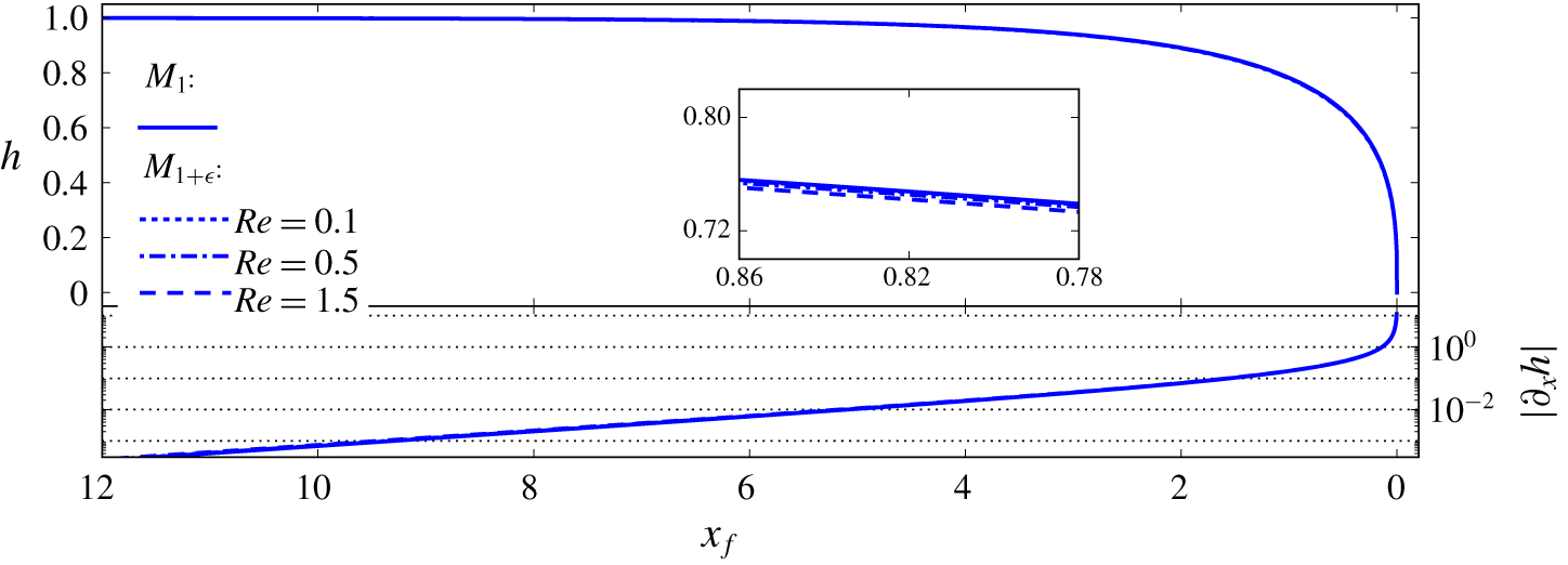
Free-surface shapes predicted by models  $M_{1}$ and
 $M_{1+\unicode[STIX]{x1D716}}$: evolution of flow height
 $h$ and derivative
 $\unicode[STIX]{x2202}_{x}h$ versus distance from the tip
 $x_{f}$. (a)
 $n=0.4$. (b)
 $n=1$. In both plots, solutions computed for two values of
 $Bi$ and two values of
 $Re$ are shown (
 $\unicode[STIX]{x1D703}=15^{\circ }$). Insets show close-ups on the slight differences among the solutions.

For computing velocity expansions at order  $O(\unicode[STIX]{x1D716})$, we consider model
 $M_{1+\unicode[STIX]{x1D716}}$ based on the
 $O(\unicode[STIX]{x1D716})$ approximation of discharge:
 $$\begin{eqnarray}M_{1+\unicode[STIX]{x1D716}}:\quad q^{(0)}\left(h_{tw},\frac{\text{d}h_{tw}}{\text{d}x_{f}}\right)+q^{(1)}\left(h_{tw},\frac{\text{d}h_{tw}}{\text{d}x_{f}},\frac{\text{d}^{2}h_{tw}}{\text{d}x_{f}^{2}}\right)=h_{tw},\end{eqnarray}$$
where the expression of  $q^{(1)}$ is provided by (2.48). Equation (3.6) constitutes a second-order ODE for
 $h_{tw}(x_{f})$. It is solved by finite-difference discretisation on a regular mesh, using the Python function newton_krylov. The same boundary condition as for model
 $M_{1}$ is considered at
 $x_{f}=0$, and we impose
 $h_{tw}\approx 1$ sufficiently far from the tip (in practice, the value provided by model
 $M_{1}$ is taken). The iterations of the relaxation algorithm are initiated with the solution of model
 $M_{1}$.
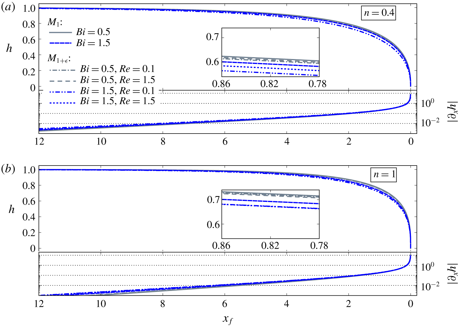
Figure 2 shows comparisons between the free surfaces obtained with models  $M_{1}$ and
 $M_{1+\unicode[STIX]{x1D716}}$ for different values of numbers
 $Bi$ and
 $Re$. In all cases, the front is steep and perpendicular to the channel bottom at the tip, namely
 $|\unicode[STIX]{x2202}_{x}h|\rightarrow \infty$ as
 $x_{f}\rightarrow 0$. Values of the derivative
 $|\unicode[STIX]{x2202}_{x}h|$ exceed 0.1 for
 $x_{f}<1.5$–2, typically, a position below which the validity of the thin-layer assumption may thus become questionable (see § 5.2). Note, however, that values of
 $|\unicode[STIX]{x2202}_{x}h|$ in excess of 1 are reached only very close to the tip, for
 $x_{f}<0.1$ typically. Away from the tip, the free surface monotonically increases towards the asymptotic value of 1, corresponding to a steady uniform regime. Flow height can be considered as essentially uniform for
 $x_{f}>10$, typically.
Globally, it appears that the free surfaces predicted by models  $M_{1}$ and
 $M_{1+\unicode[STIX]{x1D716}}$ remain very close, regardless of the parameter values considered (figure 2). Note that model
 $M_{1}$ only depends on Bingham number
 $Bi$, whereas model
 $M_{1+\unicode[STIX]{x1D716}}$ depends on both
 $Bi$ and
 $Re$. For
 $n=0.4$ (figure 2a), and when
 $Bi$ is small, the free surfaces obtained with the two models are hardly distinguishable. When
 $Bi$ increases, small deviations between the different solutions become visible. It is observed that the free surfaces computed with model
 $M_{1+\unicode[STIX]{x1D716}}$ systematically lie below those obtained with model
 $M_{1}$. Moreover, for a given value of
 $Bi$, the differences between the
 $M_{1}$ and the
 $M_{1+\unicode[STIX]{x1D716}}$ solutions are larger when
 $Re$ is small. Similar observations are made for
 $n=1$ (figure 2b).
Let us note that, far from the tip ( $x_{f}\rightarrow \infty$), expression (2.23) for the leading-order velocity in the pseudo-plug can be approximated as
 $$\begin{eqnarray}u_{pl}^{(0)}\approx \frac{n}{n+1}\unicode[STIX]{x1D706}^{1/n}\left(h-\frac{Bi}{\unicode[STIX]{x1D706}}\right)^{(n+1)/n}.\end{eqnarray}$$
Accordingly,  $\operatorname{sgn}(\unicode[STIX]{x2202}_{x}u_{pl}^{(0)})=\operatorname{sgn}(\unicode[STIX]{x2202}_{x}h)=-1$ for
 $x_{f}\rightarrow \infty$. The factor
 $\operatorname{sgn}(\unicode[STIX]{x2202}_{x}u_{pl}^{(0)})$, which is assumed to be constant (see § 2.5.3), is therefore taken as uniformly equal to
 $-1$ along the flow for computing solutions of model
 $M_{1+\unicode[STIX]{x1D716}}$.
3.2 Velocity profiles and free-surface velocity
Approximations of the velocity profile  $u(y)$ at leading-order and at
 $O(\unicode[STIX]{x1D716})$ are computed from expressions (2.22) and (2.47). When limiting to leading order, free surfaces obtained from model
 $M_{1}$ are considered. Conversely, for computing velocity approximations at
 $O(\unicode[STIX]{x1D716})$, free surfaces coming from model
 $M_{1+\unicode[STIX]{x1D716}}$ are taken into account. Considering these two, slightly different, free-surface models ensures that all computed velocity profiles effectively comply with the condition
 $\bar{u}=1$. In the following, for convenience, the terminology
 $M_{1}$ and
 $M_{1+\unicode[STIX]{x1D716}}$ is also used for referring to the velocity profiles computed with either of the models. Again, the assumption
 $\operatorname{sgn}(\unicode[STIX]{x2202}_{x}u_{pl}^{(0)})=-1$ is made to evaluate the normal-stress correction terms. It was checked that the reconstructed
 $O(\unicode[STIX]{x1D716})$ velocity profiles are effectively consistent with this assumption, namely that values of
 $u_{pl}^{(0)}$ calculated with model
 $M_{1+\unicode[STIX]{x1D716}}$ are decreasing towards the tip.
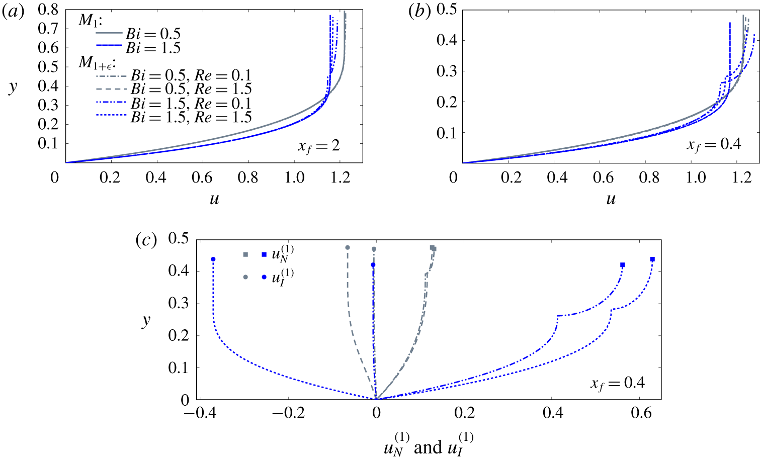
Figure 3(a,b) present velocity profiles calculated for two values of  $x_{f}$ and different values of
 $Bi$ and
 $Re$. Only the case
 $n=0.4$ is shown here. Obviously, sufficiently far from the tip, velocities obtained with models
 $M_{1}$ and
 $M_{1+\unicode[STIX]{x1D716}}$ are essentially identical. At
 $x_{f}=2$, slight differences between the predictions of the two models begin to appear for large values of
 $Bi$ (figure 3a). These differences between the models are then magnified when moving closer to the tip, as shown in figure 3(b) for
 $x_{f}=0.4$. The vertical variations of velocity in the pseudo-plug predicted by model
 $M_{1+\unicode[STIX]{x1D716}}$ are also clearly visible. Note that the corresponding velocity profiles present a nonphysical kink at
 $y=h-h_{p}$. As discussed in the following (see § 5.1), this singularity arises from the patching of the
 $O(\unicode[STIX]{x1D716})$ correction terms at the fake yield surface.
(a,b) Vertical profiles of longitudinal velocity  $u$ computed with models
 $M_{1}$ and
 $M_{1+\unicode[STIX]{x1D716}}$ at two distances from the tip
 $x_{f}$ (see the legend). In both plots, solutions computed for two values of
 $Bi$ and two values of
 $Re$ are shown (
 $\unicode[STIX]{x1D703}=15^{\circ }$,
 $n=0.4$). (c) Vertical profiles of the
 $O(\unicode[STIX]{x1D716})$ normal-stress (thick lines with squares) and inertia (thin lines with circles) correction terms
 $u_{N}^{(1)}$ and
 $u_{I}^{(1)}$ at a position
 $x_{f}=0.4$.

Globally, the interplay of numbers  $Bi$ and
 $Re$ on the velocity profiles is rather complex. Depending on the values of these parameters, and on the vertical position
 $y$, velocities predicted by model
 $M_{1+\unicode[STIX]{x1D716}}$ can either be larger or smaller than those predicted by model
 $M_{1}$. Figure 3(c) shows the typical relative magnitudes of the
 $O(\unicode[STIX]{x1D716})$ normal-stress and inertia correction terms
 $u_{N}^{(1)}$ and
 $u_{I}^{(1)}$. These two correction terms generally display opposite signs (except for very low values of
 $Bi$). The normal-stress term
 $u_{N}^{(1)}$ is positive and, as expected, increases with the Bingham number
 $Bi$. The inertia term
 $u_{I}^{(1)}$ is generally negative, and its absolute value increases with the Reynolds number
 $Re$. More surprisingly, the inertia correction also appears to significantly increase (in absolute value) with
 $Bi$. The counterbalancing effects between the two correction terms explain that, for a given value of
 $Bi$, the net velocity correction tends to decrease when
 $Re$ increases (clearly visible in figure 3b). The net correction, however, systematically increases with
 $Bi$ (as seen in figure 3a,b).
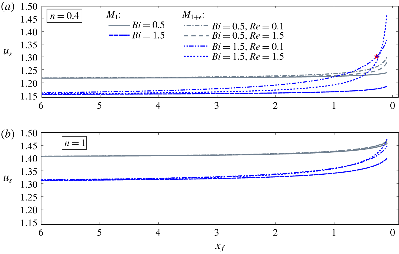
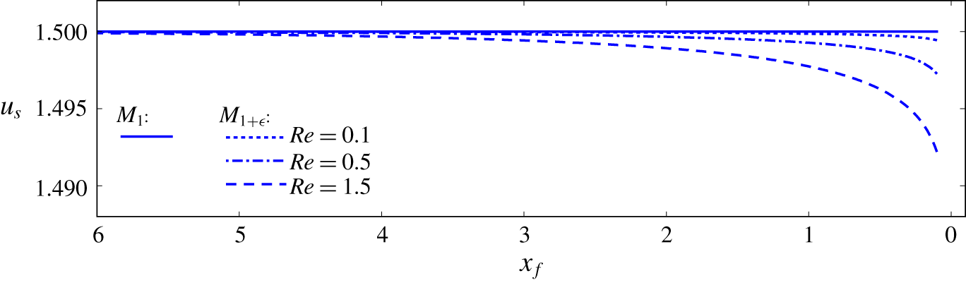
Figure 4 presents the evolution of free-surface velocity  $u_{s}$ along the surge. For model
 $M_{1}$,
 $u_{s}=u_{pl}^{(0)}$, whereas for model
 $M_{1+\unicode[STIX]{x1D716}}$,
 $u_{s}=u_{pl}^{(0)}+u_{pl}^{(1)}|_{y=h}$. Computed predictions have been truncated at
 $x_{f}=0.1$, that is, at the position where
 $|\unicode[STIX]{x2202}_{x}h|$ typically reaches a value of 1 (see figure 2). It was checked that, with model
 $M_{1+\unicode[STIX]{x1D716}}$, the asymptotic expansion remains well-ordered, that is,
 $u_{s}^{(1)}<u_{s}^{(0)}$, for
 $x_{f}>0.1$ in all but one of the displayed cases. With
 $n=0.4$,
 $Bi=1.5$ and
 $Re=0.1$, the expansion ceases to be well-ordered at
 $x_{f}=0.25$, typically (red star in figure 4a). Globally, it is observed that, for the two models and all considered parameter values, surface velocity
 $u_{s}$ systematically increases towards the tip. Note that the increase of
 $u_{s}$ is not incompatible with the requirement that
 $\operatorname{sgn}(\unicode[STIX]{x2202}_{x}u_{pl}^{(0)})=-1$ in model
 $M_{1+\unicode[STIX]{x1D716}}$ (see § 3.1). Again, the counterbalancing effects of the
 $O(\unicode[STIX]{x1D716})$ normal-stress and inertia correction terms are clearly apparent for
 $n=0.4$ (figure 4a): the normal-stress correction tends to increase the value of
 $u_{s}$, whereas the inertia term generally acts in the opposite direction. The net correction, however, remains systematically positive: surface velocities obtained with model
 $M_{1+\unicode[STIX]{x1D716}}$ are larger than those obtained with model
 $M_{1}$, with differences becoming visible for
 $x_{f}<2-6$, typically. For similar values of
 $Bi$ and
 $Re$, the influence of the
 $O(\unicode[STIX]{x1D716})$ corrections, and notably of the inertia term, appear to be less marked in the case
 $n=1$ (figure 4b).
Evolution of free-surface velocity  $u_{s}$ predicted by models
 $M_{1}$ and
 $M_{1+\unicode[STIX]{x1D716}}$ as a function of distance from the tip
 $x_{f}$: (a)
 $n=0.4$; (b)
 $n=1$. In both plots, solutions computed for two values of
 $Bi$ and two values of
 $Re$ are shown (
 $\unicode[STIX]{x1D703}=15^{\circ }$). In (a), the red star marks the position where the asymptotic expansion in model
 $M_{1+\unicode[STIX]{x1D716}}$ ceases to be well-ordered for the case
 $Bi=1.5$,
 $Re=0.1$ (blue dot-dashed line).

3.3 Pseudo-plug shear rate and effective unsheared layer
At  $O(\unicode[STIX]{x1D716})$, a strictly positive shear rate
 $|\dot{\unicode[STIX]{x1D6FE}}|$ is predicted in the pseudo-plug (see § 2.4). Integrating (2.31), the following expression is obtained for the
 $O(\unicode[STIX]{x1D716})$ vertically averaged shear rate
 $|\dot{\unicode[STIX]{x1D6FE}}|_{pl}^{(1)}$ in the pseudo-plug:
 $$\begin{eqnarray}|\dot{\unicode[STIX]{x1D6FE}}|_{pl}^{(1)}=\unicode[STIX]{x03C0}|\unicode[STIX]{x2202}_{x}u_{pl}^{(0)}|.\end{eqnarray}$$
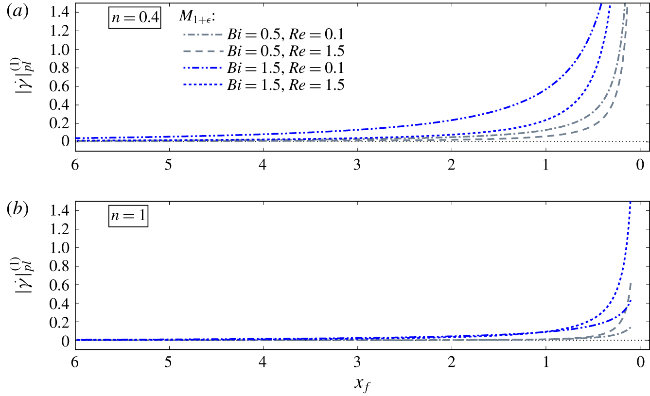
As shown in figure 5, values of  $|\dot{\unicode[STIX]{x1D6FE}}|_{pl}^{(1)}$ obtained from model
 $M_{1+\unicode[STIX]{x1D716}}$ significantly depart from 0 for
 $x_{f}<2-6$, depending on the considered values of
 $Bi$ and
 $Re$. Again, note that the plots are truncated at
 $x_{f}=0.1$. The increase in
 $|\dot{\unicode[STIX]{x1D6FE}}|_{pl}^{(1)}$ towards the tip is primarily driven by the normal-stress correction, and is more pronounced for larger
 $Bi$. Conversely, for
 $n=0.4$, the increase of
 $|\dot{\unicode[STIX]{x1D6FE}}|_{pl}^{(1)}$ becomes generally confined closer and closer to the tip when
 $Re$ increases (counterbalancing effect, see figure 5a). For
 $n=1$, the net
 $O(\unicode[STIX]{x1D716})$ correction is less pronounced, and the effect of
 $Re$ changes sign in the close vicinity of the tip (figure 5b).
Evolution of  $O(\unicode[STIX]{x1D716})$ vertically averaged shear rate in the pseudo-plug
 $|\dot{\unicode[STIX]{x1D6FE}}|_{pl}^{(1)}$ predicted by model
 $M_{1+\unicode[STIX]{x1D716}}$, as a function of distance from the tip
 $x_{f}$: (a)
 $n=0.4$; (b)
 $n=1$. In both plots, solutions computed for two values of
 $Bi$ and two values of
 $Re$ are shown (
 $\unicode[STIX]{x1D703}=15^{\circ }$). The dotted line indicates the 0 value (i.e.
 $M_{1}$ solution).

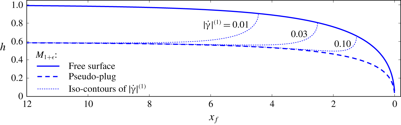
Figure 6 displays a typical example of iso-contours of the  $O(\unicode[STIX]{x1D716})$ shear rate
 $|\dot{\unicode[STIX]{x1D6FE}}|^{(1)}$ in the pseudo-plug. Recall that the pseudo-plug corresponds to an unsheared layer for the leading-order approximation. Similarly, one can define an effective unsheared layer at order
 $O(\unicode[STIX]{x1D716})$, as the zone located above the particular
 $|\dot{\unicode[STIX]{x1D6FE}}|^{(1)}$-contour corresponding to a chosen shear-rate threshold. For sufficiently large values of
 $x_{f}$, the boundary of this effective unsheared layer coincides with the fake yield surface
 $y=h-h_{p}$, regardless of the chosen threshold. When approaching the tip, however, the thickness of the effective unsheared layer decreases much faster than
 $h_{p}$, and abruptly collapses at a certain value of
 $x_{f}$. The precise position at which this collapse occurs, moves closer to the tip as the considered shear-rate threshold increases (figure 6).
Iso-contours of  $O(\unicode[STIX]{x1D716})$ shear rate
 $|\dot{\unicode[STIX]{x1D6FE}}|^{(1)}$ in the pseudo-plug predicted by model
 $M_{1+\unicode[STIX]{x1D716}}$ (dotted lines). The solid line represents the free-surface and the dashed line represents the fake yield surface
 $y=h-h_{p}$ (
 $Bi=1.5$,
 $Re=1.5$,
 $\unicode[STIX]{x1D703}=15^{\circ }$,
 $n=0.4$).

4 Comparison with experimental results
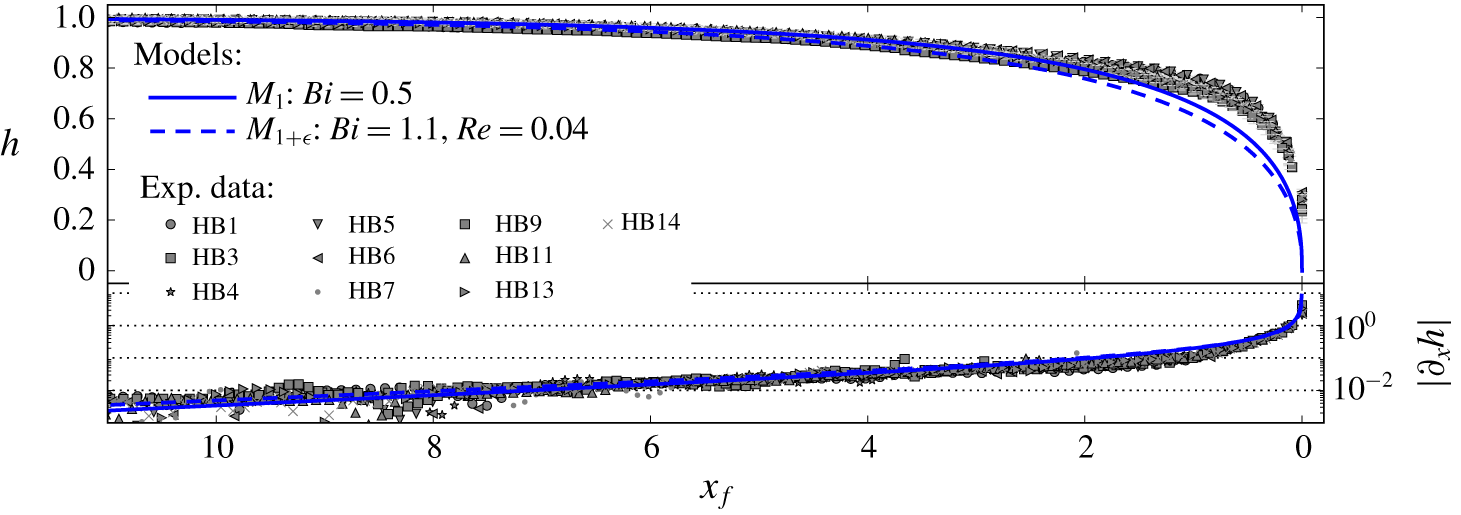
In this section, the leading-order and  $O(\unicode[STIX]{x1D716})$ velocity approximations are cross-compared with experimental results. The experimental dataset consists of high-resolution measurements of the internal velocity field within laboratory viscoplastic surges (Freydier et al. Reference Freydier, Chambon and Naaim2017). In parallel, free-surface shapes were also recorded. Experimental set-up and methods were detailed in previous papers (Chambon et al. Reference Chambon, Ghemmour and Naaim2014; Freydier et al. Reference Freydier, Chambon and Naaim2017). Only the elements essential for the present comparison are recalled in the following.
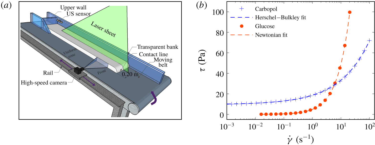
(a) Scheme of the conveyor-belt channel. The stationary surge is represented in white. (b) Typical steady-state flow curves of Carbopol and glucose samples used in the experiments: shear stress  $\unicode[STIX]{x1D70F}$ versus shear rate
 $\dot{\unicode[STIX]{x1D6FE}}$ (semi-log scale). Symbols correspond to rheometrical measurements; dashed lines represent the best-fitting Herschel–Bulkley and Newtonian laws (Carbopol:
 $\unicode[STIX]{x1D70F}_{c}=9.6~\text{Pa}$,
 $K=9.0~\text{Pa}~\text{s}^{n}$,
 $n=0.42$. Glucose:
 $\unicode[STIX]{x1D702}=5.6~\text{Pa}~\text{s}$).

4.1 Review of experimental methods
The experimental set-up consists of a 3 m long inclined channel, whose bottom is constituted by an upward-moving conveyor belt (figure 7a). Owing to this mobile bottom, gravity-driven free-surface surges that remain stationary in the laboratory reference frame can be generated. When a given volume of fluid is placed in the channel, flow height spontaneously adapts to the fixed bottom velocity  $u_{b}$ (Chambon et al. Reference Chambon, Ghemmour and Laigle2009, Reference Chambon, Ghemmour and Naaim2014). The studied surges have a typical length of 1 m and a typical height of 10–30 mm, thereby complying with thin-layer assumption (see figure 8). Side-wall effects remain limited in this set-up, such that transverse velocities are negligible and the flow can be regarded as effectively two dimensional along the centreline of the surges (except in the close vicinity of the tip: see Freydier et al. (Reference Freydier, Chambon and Naaim2017)).
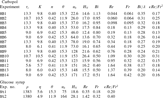
Characteristics of the experiments performed with Carbopol and glucose syrup: fluid density  $\unicode[STIX]{x1D70C}$ (
 $\text{kg}~\text{m}^{-3}$: only indicated for glucose, taken at
 $1000~\text{kg}~\text{m}^{-3}$ for Carbopol), yield stress
 $\unicode[STIX]{x1D70F}_{c}$ (Pa; for Carbopol), consistency
 $K$ (
 $\text{Pa}~\text{s}^{n}$; for Carbopol), power-law index
 $n$ (for Carbopol), viscosity
 $\unicode[STIX]{x1D702}$ (
 $\text{Pa}~\text{s}$; for glucose), slope angle (deg.), bottom belt velocity
 $u_{b}$ (
 $\text{mm}~\text{s}^{-1}$), steady uniform height
 $H_{N}$ (mm), Bingham number
 $Bi$ (for Carbopol), Reynolds number
 $Re$, Froude number
 $Fr$, plug thickness in uniform regions
 $Bi/\unicode[STIX]{x1D706}$ (for Carbopol) and number
 $\unicode[STIX]{x1D716}Re/Fr^{2}$.

Viscoplastic experiments were performed with Carbopol (EDT 2623). Even if it can display more complex rheological trends in transient flows, this polymeric micro-gel was used as a model viscoplastic fluid in numerous previous studies (e.g. Piau Reference Piau2007; Bonn et al. Reference Bonn, Denn, Berthier, Divoux and Manneville2017). As shown in figure 7(b), the steady-state flow curve of the material is well represented by the Herschel–Bulkley law. The yield stress  $\unicode[STIX]{x1D70F}_{c}$, consistency
 $K$ and power index
 $n$ of the samples were determined using a laboratory rheometer (Bohlin CVOR) equipped with roughened parallel-plate tools to avoid slip. Values of
 $n$ systematically lie around 0.4 (see table 1). Following our previous works (Chambon et al. Reference Chambon, Ghemmour and Naaim2014; Freydier et al. Reference Freydier, Chambon and Naaim2017), measured values of
 $\unicode[STIX]{x1D70F}_{c}$ and
 $K$ were increased by 11 % and 19 %, respectively, to ensure quantitative agreement between predictions and measurements of flow height
 $H_{N}$ in the uniform zone of the surges, far from the tip.
A few benchmark experiments were also performed with a Newtonian fluid (glucose syrup). In this case, the viscosity  $\unicode[STIX]{x1D702}$ of the samples was measured with a cone-plate geometry (figure 7b). As glucose viscosity strongly depends on temperature (Schellart Reference Schellart2011), particular care was taken to perform experiments as rapidly as possible, and avoid temperature variations, when working with this material. Results obtained with Newtonian surges are summarised in appendix B.
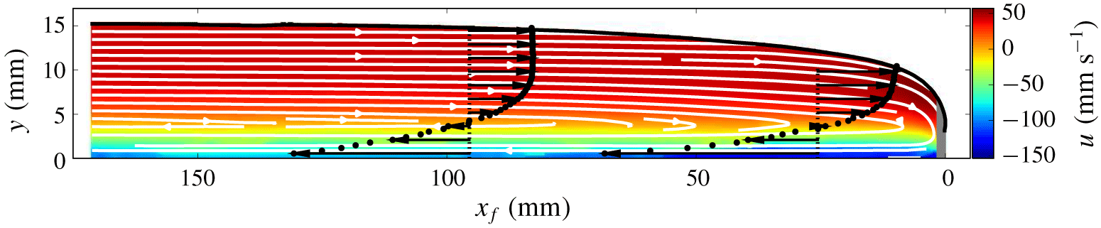
Measured longitudinal velocity ( $u$) field for experiment HB13 (
 $Bi=0.5$,
 $Re=1.4$). The colour scale corresponds to raw velocity values (no shifting by bed velocity
 $u_{b}$). Streamlines are superimposed in white. Two vertical profiles of
 $u$, obtained at positions
 $x_{f}=95~\text{mm}$ and
 $x_{f}=25~\text{mm}$, respectively, are also represented. The grey area close to the tip indicates the zone where no reliable velocity measurements could be obtained.

Flows were monitored by illuminating the centreplane of the surges with a laser sheet, and acquiring images from the side with a 500 Hz camera. The transparent fluids are seeded with  $10~\unicode[STIX]{x03BC}\text{m}$ tracers. We reconstruct velocity fields (see figure 8) through a space–time analysis technique that takes full advantage of the stationary character of the surges (Freydier et al. Reference Freydier, Chambon and Naaim2017). This technique achieves higher spatial resolutions than more classical correlation methods (such as particle image velocimetry (PIV)), with typical values in our experiments of 1.24 mm in the longitudinal direction and 0.62 mm in the vertical direction. In addition, local flow height and free-surface shape are also extracted from the images, with an uncertainty in the range
 $\pm 0.2{-}0.9~\text{mm}$.
An example of measured longitudinal velocity field is shown in figure 8. Far from the tip, the velocity profiles present the typical two-layer shape expected in a steady uniform regime, with an unsheared plug close to the free surface and a sheared layer underneath. When approaching the tip, velocity profiles begin to display shear throughout the entire depth of the flow. Accordingly, the unsheared zone seemingly disappears for  $x_{f}/H_{N}<1-2$, typically (Freydier et al. Reference Freydier, Chambon and Naaim2017). Experimental measurements also feature an increase in surface velocity when approaching the tip (figure 8).
4.2 Strategy of experimental–theoretical comparisons
For this study, results coming from 14 different experiments with Carbopol and two different experiments with glucose were aggregated (see table 1). These experiments were performed with different bottom velocities  $u_{b}$ (in the range
 $25{-}150~\text{mm}~\text{s}^{-1}$), different slope angles
 $\unicode[STIX]{x1D703}$ (
 $11.9^{\circ }$ and
 $15.3^{\circ }$), and different batches of Carbopol and glucose syrup. The yield stress
 $\unicode[STIX]{x1D70F}_{c}$ of Carbopol samples varied between 5 and 12 Pa. Accordingly, values of
 $Bi$ and
 $Re$ achieved in the viscoplastic experiments spanned the ranges 0.4–1.1 and 0.04–1.6, respectively. Note that, in practice, numbers
 $Bi$ and
 $Re$ tend to be inversely correlated in the experiments, such that high (respectively, low) values of
 $Bi$ are generally associated with low (respectively, high) values of
 $Re$ (table 1). For the Newtonian experiments, the viscosity of glucose samples varied between 5 and
 $8~\text{Pa}~\text{s}$, leading to values of
 $Re$ in the range 0.4–1.4. Overall, the values of
 $\unicode[STIX]{x1D716}Re/Fr^{2}$ are between
 $0.1$ and
 $0.4$. Although somewhat smaller than 1, these values are systematically larger than
 $\unicode[STIX]{x1D716}$ (calculated for a typical length of 1 m) by at least one order of magnitude, indicating that the experiments effectively comply with the flow regime considered in this study (see § 2.2). Lastly, for reference, values of
 $Fr$ and
 $Bi/\unicode[STIX]{x1D706}$ (plug thickness in uniform regions) are also indicated in table 1.
In the reference frame attached to channel bottom, the stationary surges generated in our set-up correspond to travelling waves propagating at belt velocity  $u_{b}$. Direct comparisons with theoretical predictions of models
 $M_{1}$ and
 $M_{1+\unicode[STIX]{x1D716}}$ obtained in § 3, can thus be performed. To that aim, experimental measurements of longitudinal velocity
 $u$ are shifted by the value of
 $u_{b}$. Owing to an experimental artefact, the depth-averaged velocities
 $\bar{u}$ obtained by integration of the shifted velocity profiles may differ from the expected value
 $u_{b}$ by a few per cent (Freydier et al. Reference Freydier, Chambon and Naaim2017). To normalise experimental data consistently with theoretical predictions, measured velocities are thus rescaled by the actual, experimental values of
 $\bar{u}$ (constant along the surges). Similarly, positions
 $x_{f}$ and
 $y$ are rescaled by the value of uniform height
 $H_{N}$ directly measured on the surges, far from the tip.
Owing to the non-physical kink at the fake yield surface in the theoretical velocity profiles at order  $O(\unicode[STIX]{x1D716})$ (see § 3.2), detailed comparisons with the experimental velocity profiles were not attempted in the viscoplastic case. Comparisons presented hereafter shall thus concentrate on (i) surface velocity
 $u_{s}$ and (ii) vertically averaged shear rate in the pseudo-plug layer
 $|\dot{\unicode[STIX]{x1D6FE}}|_{pl}$. Note that we expect the evolution of
 $|\dot{\unicode[STIX]{x1D6FE}}|_{pl}$ along the surge to be essentially unaffected by the singularity at
 $y=h-h_{p}$, because this quantity only depends on the longitudinal derivative
 $\unicode[STIX]{x2202}_{x}u_{pl}^{(0)}$ (see (3.8)).
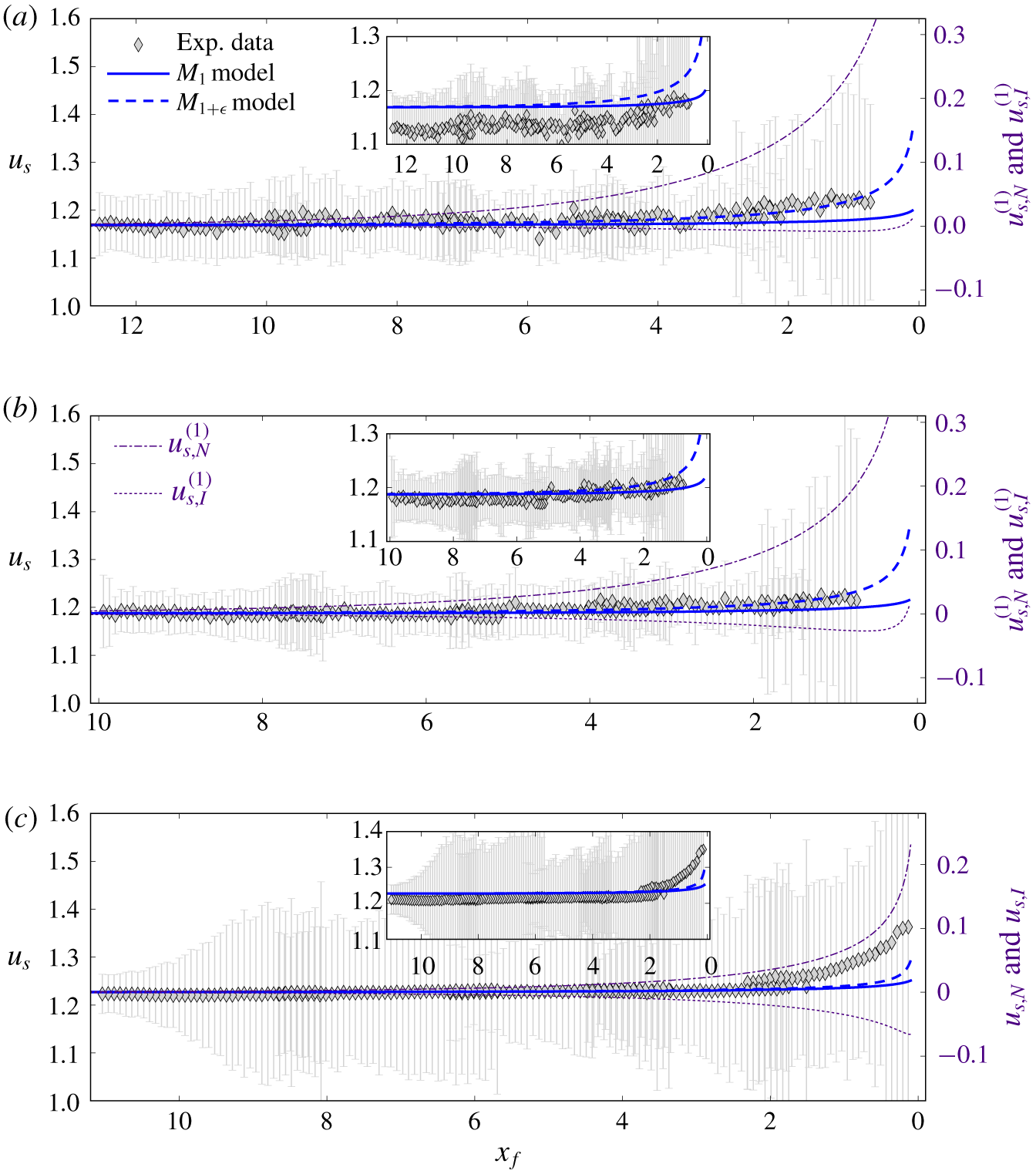
Free-surface velocity  $u_{s}$ as a function of distance from the tip
 $x_{f}$, comparison between experimental data and predictions of models
 $M_{1}$ and
 $M_{1+\unicode[STIX]{x1D716}}$: (a)
 $Bi=1.1$,
 $Re=0.04$ (experiment HB1); (b)
 $Bi=0.8$ and
 $Re=0.2$ (experiment HB4); (c)
 $Bi=0.5$ and
 $Re=1.4$ (experiment HB13). Error bars correspond to velocity measurement uncertainties. Light purple dotted and dot-dashed lines show contributions of the
 $O(\unicode[STIX]{x1D716})$ normal-stress and inertia correction terms
 $u_{s,N}^{(1)}$ and
 $u_{s,I}^{(1)}$, respectively (scale on the right axis). Insets display actual experimental data, whereas the main panels show data corrected by a slight vertical shift (see the text).

4.3 Free-surface velocity
Figure 9 shows comparisons between experimental surface velocities and predictions of models  $M_{1}$ and
 $M_{1+\unicode[STIX]{x1D716}}$. Note that raw
 $u_{s}$ measurements generally present a slight systematic discrepancy with theoretical predictions far from the tip (see insets). This discrepancy, comprised within experimental errors, is attributed to uncertainties on the rheological parameters and, thus, on experimental
 $Bi$ values (see figure 4, in which the dependence of
 $u_{s}$ predictions upon
 $Bi$ is clearly observed). To better compare the modelled and experimental trends in the vicinity of the tip, datapoints in the main panel of figure 9 have been shifted slightly, so as to match theoretical predictions in the uniform zone.
As explained in § 3, differences between predictions of models  $M_{1}$ and
 $M_{1+\unicode[STIX]{x1D716}}$ get more pronounced when the Bingham number
 $Bi$ increases. Hence, let us first focus on an experiment characterised by a relatively large value of
 $Bi$ and a small value of
 $Re$ (figure 9a). In this case, it is clearly observed that experimental values of
 $u_{s}$ increase faster than predictions of model
 $M_{1}$ when approaching the tip, with discrepancies becoming apparent for
 $x_{f}<2$ typically. In contrast, experimental measurements are in good agreement with model
 $M_{1+\unicode[STIX]{x1D716}}$, even for the lowest values of
 $x_{f}$ at which measurements are available. The magnitudes of the
 $O(\unicode[STIX]{x1D716})$ normal-stress and inertia correction terms are also represented in the figure. As expected, for this experiment, the
 $O(\unicode[STIX]{x1D716})$ correction is dominated by the normal-stress term, whereas the inertia term remains much smaller and close to zero.
The better agreement provided by model  $M_{1+\unicode[STIX]{x1D716}}$ close to the tip is also visible, though to a lesser extent, in figure 9(b), which corresponds to an experiment with a lower value of
 $Bi$ and a larger value of
 $Re$. Here, the magnitude of the inertia correction term is larger than in figure 9(a), such that the net difference between models
 $M_{1}$ and
 $M_{1+\unicode[STIX]{x1D716}}$ is less pronounced. Experimental data could be viewed as agreeing with either one of the two models, although the predictions of model
 $M_{1+\unicode[STIX]{x1D716}}$ again appear to better capture the increasing trend close to the tip.
Finally, figure 9(c) shows the case of a large  $Re$ number, for which the inertia and normal-stress correction terms are almost of the same order. Here, predictions of the
 $M_{1}$ and
 $M_{1+\unicode[STIX]{x1D716}}$ models are essentially indistinguishable. Experimental data, however, deviate from these predictions close to the tip. Note that measurements seem to follow the evolution of the normal-stress correction term, suggesting that the inertia correction might be overestimated in this case.
To obtain a synthetic view of all experiments performed, the following error ratio was computed:
 $$\begin{eqnarray}r_{E}=\frac{|u_{s}^{exp}-u_{s}^{M_{1+\unicode[STIX]{x1D716}}}|}{|u_{s}^{exp}-u_{s}^{M_{1}}|},\end{eqnarray}$$
where  $u_{s}^{exp}$ denotes the experimental surface velocity, and
 $u_{s}^{M_{1}}$ and
 $u_{s}^{M_{1+\unicode[STIX]{x1D716}}}$ denote the surface velocities predicted by models
 $M_{1}$ and
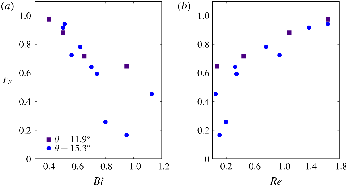
 $M_{1+\unicode[STIX]{x1D716}}$, respectively. Figure 10 shows values of
 $r_{E}$ obtained at
 $x_{f}=0.7$ as a function of
 $Bi$ and
 $Re$ numbers. Similar trends are obtained at other values of
 $x_{f}$, as long as positions sufficiently close to the tip are considered. First, it is observed that
 $r_{E}$ displays values lower than 1, indicating that the match provided by model
 $M_{1+\unicode[STIX]{x1D716}}$ is systematically better than that obtained with model
 $M_{1}$. Moreover, the larger the values of
 $Bi$ (or, correlatively, the lower the values of
 $Re$), the closer to 0 the values of
 $r_{E}$. This reflects an excellent agreement between experimental data and predictions of model
 $M_{1+\unicode[STIX]{x1D716}}$ for large
 $Bi$ values. In contrast, for low values of
 $Bi$ (or large values of
 $Re$), the ratio
 $r_{E}$ remains close to 1, meaning that the improvement brought by the
 $O(\unicode[STIX]{x1D716})$ correction terms is relatively marginal in this case. In this limit of low
 $Bi$ values, experimental data show significant discrepancies with both
 $M_{1}$ and
 $M_{1+\unicode[STIX]{x1D716}}$ models.
Error ratio  $r_{E}$ (see the text) computed at
 $x_{f}=0.7$ as a function of (a) the Bingham number
 $Bi$ and (b) the Reynolds number
 $Re$, for the 14 experiments performed with Carbopol (see table 1).

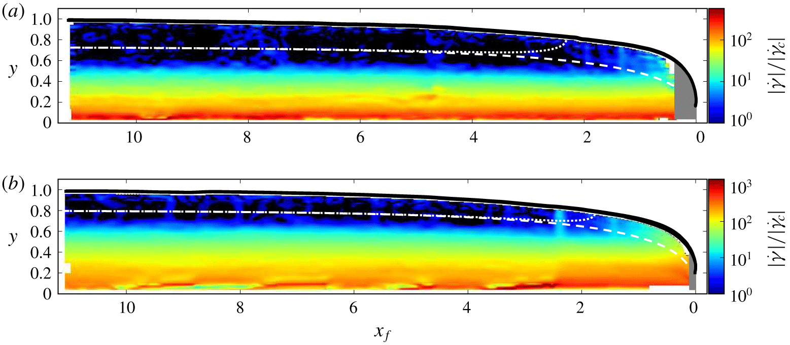
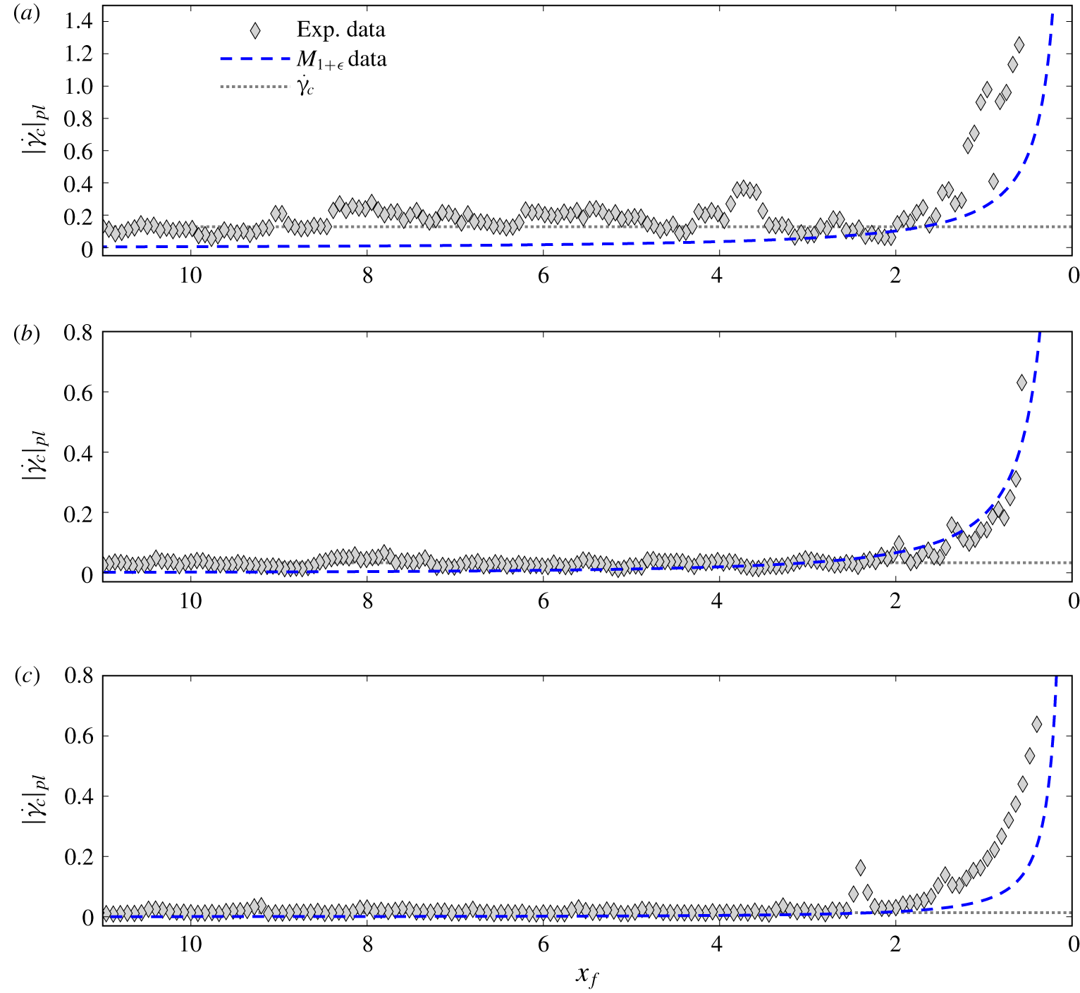
Experimental shear rate  $|\dot{\unicode[STIX]{x1D6FE}}|$ normalised by typical measurement noise level
 $\dot{\unicode[STIX]{x1D6FE}}_{c}$: (a)
 $Bi=0.7$,
 $Re=0.3$ (experiment HB7,
 $\dot{\unicode[STIX]{x1D6FE}}_{c}=0.033$); (b)
 $Bi=0.5$,
 $Re=1.4$ (experiment HB13,
 $\dot{\unicode[STIX]{x1D6FE}}_{c}=0.013$). The white dashed line represents the fake yield surface predicted by model
 $M_{1+\unicode[STIX]{x1D716}}$ (essentially indistinguishable from that predicted by model
 $M_{1}$), and the white dotted line represents the predicted iso-contour
 $|\dot{\unicode[STIX]{x1D6FE}}|^{(1)}=\dot{\unicode[STIX]{x1D6FE}}_{c}$ in the pseudo-plug (see § 3.3).

Vertically averaged shear rate in the pseudo-plug  $|\dot{\unicode[STIX]{x1D6FE}}|_{pl}$ as a function of distance from the tip
 $x_{f}$, comparison between experimental data and predictions of model
 $M_{1+\unicode[STIX]{x1D716}}$: (a)
 $Bi=0.95$,
 $Re=0.06$ (experiment HB2); (b)
 $Bi=0.7$,
 $Re=0.3$ (experiment HB7); (c)
 $Bi=0.5$,
 $Re=1.4$ (experiment HB13). The grey dashed line indicates the typical level of measurement noise
 $\dot{\unicode[STIX]{x1D6FE}}_{c}$.

4.4 Pseudo-plug shear rate
Figure 11 shows examples of shear rate  $|\dot{\unicode[STIX]{x1D6FE}}|$ computed by direct differentiation of the measured velocity fields (accounting for vertical and longitudinal derivative terms). To improve clarity, values of
 $|\dot{\unicode[STIX]{x1D6FE}}|$ are normalised by the typical level of experimental noise
 $\dot{\unicode[STIX]{x1D6FE}}_{c}$ (variable among the experiments), and the colour scale is thresholded for
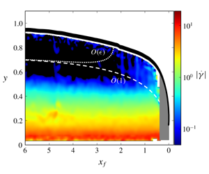
 $|\dot{\unicode[STIX]{x1D6FE}}|/\dot{\unicode[STIX]{x1D6FE}}_{c}<1$. Hence, dark-blue/black areas correspond to the apparent unsheared layer that can be determined from the experiments. Far from the tip, this apparent unsheared layer is thicker than the predicted pseudo-plug, owing to the thresholding at
 $\dot{\unicode[STIX]{x1D6FE}}_{c}$. In the tip region, in contrast, it is observed that the experimental unsheared layer thins much faster than the pseudo-plug, and disappears for
 $x_{f}<1$–2 typically. Interestingly, this feature appears to be consistent with the abrupt collapse of the effective unsheared layer obtained from model
 $M_{1+\unicode[STIX]{x1D716}}$ (see § 3.3). If this theoretical effective unsheared layer is defined on the base of the iso-value of the shear rate corresponding to measurement noise
 $\dot{\unicode[STIX]{x1D6FE}}_{c}$, both the overall shape of the layer and the location of the collapse appear in reasonable agreement with experimental data (figure 11).
More quantitatively, figure 12 compares the evolution of the vertically averaged shear rate  $|\dot{\unicode[STIX]{x1D6FE}}|_{pl}$ measured in the pseudo-plug with predictions of model
 $M_{1+\unicode[STIX]{x1D716}}$. As for their theoretical counterparts (see § 3.3), experimental values of
 $|\dot{\unicode[STIX]{x1D6FE}}|_{pl}$ are computed by averaging all
 $|\dot{\unicode[STIX]{x1D6FE}}|$ measurements obtained within the boundaries of the theoretical pseudo-plug for a given position
 $x_{f}$. In agreement with the model, a clear increase of
 $|\dot{\unicode[STIX]{x1D6FE}}|_{pl}$ in the vicinity of the tip is visible in the data. Measurements appear to be nicely captured by the theoretical predictions for small to moderate values of
 $Re$ (figure 12a,b). Note that the slightly less compelling agreement observed for the largest value of
 $Bi$ (figure 12a), can be explained by a larger noise level for this experiment. Conversely, as for surface velocities, predictions of model
 $M_{1+\unicode[STIX]{x1D716}}$ appear to underestimate the data for large values of
 $Re$ (figure 12c).
5 Discussion
To the best of the authors’ knowledge, this article presents the first complete asymptotic expansion, up to order  $O(\unicode[STIX]{x1D716})$, of longitudinal velocity
 $u$ and flow discharge
 $q$ in a thin free-surface viscoplastic surge. Our analysis expands on the previous work of Fernandez-Nieto et al. (Reference Fernandez-Nieto, Noble and Vila2010) in two respects: (i) the general case of a Herschel–Bulkley constitutive law (with
 $n>0$) is treated; and (ii) we consider a flow regime in which
 $\unicode[STIX]{x1D716}Re/Fr^{2}=O(1)$, whereas this term was regarded as
 $O(\unicode[STIX]{x1D716})$ by Fernandez-Nieto et al. (Reference Fernandez-Nieto, Noble and Vila2010). This latter assumption provides more flexibility to the leading-order solution, which coincides with a lubrication approximation characterised by a variable pseudo-plug thickness
 $h_{p}$ depending on
 $\unicode[STIX]{x2202}_{x}h$. Such a feature is required to model, for example, surge fronts, in which pseudo-plug thickness cannot be regarded as constant. This flow regime also matches that typically achieved in the experiments used for comparisons in § 4. As a counterpart, the assumption
 $\unicode[STIX]{x1D716}Re/Fr^{2}=O(1)$ leads to the appearance of factors proportional to
 $\unicode[STIX]{x2202}_{x}h_{p}$ and
 $\unicode[STIX]{x2202}_{t}h_{p}$ in the
 $O(\unicode[STIX]{x1D716})$ correction terms. It is straightforward to check that the expressions of correction terms derived in § 2 effectively reduce to those obtained by Fernandez-Nieto et al. (Reference Fernandez-Nieto, Noble and Vila2010) when setting
 $\unicode[STIX]{x1D716}Re/Fr^{2}=0$ (and, thus, replacing
 $\unicode[STIX]{x1D6EC}$ by
 $\unicode[STIX]{x1D706}$ and cancelling out all terms in
 $\unicode[STIX]{x2202}_{x,t}\unicode[STIX]{x1D6EC}$).
5.1 Influence of $O(\unicode[STIX]{x1D716})$ correction terms

Two sets of  $O(\unicode[STIX]{x1D716})$ correction terms, with different physical origins, affect the asymptotic expansions of
 $u$ and
 $q$. Correction terms related to inertia effects also arise in the case of Newtonian or power-law fluids (Fernandez-Nieto et al. Reference Fernandez-Nieto, Noble and Vila2010; Noble & Vila Reference Noble and Vila2013; Boutounet et al. Reference Boutounet, Monnier and Vila2016). Normal-stress correction terms, in contrast, are specific to the viscoplastic character of the fluid, because they are directly related to the existence of the pseudo-plug layer. Note that in the flow regime considered here, and unlike in the work of Fernandez-Nieto et al. (Reference Fernandez-Nieto, Noble and Vila2010), these normal-stress corrections affect the velocity profile in both the pseudo-plug and the sheared layer underneath.
The relative influence of these  $O(\unicode[STIX]{x1D716})$ correction terms was investigated in the specific case of travelling-wave solutions, focusing on the tip region. The free-surface shape was shown to be only weakly sensitive to
 $O(\unicode[STIX]{x1D716})$ corrections, regardless of the considered
 $Bi$ and
 $Re$ values (see figure 2). However, a significant effect of both inertia and normal-stress correction terms was observed on the velocity profiles, all the more for small values of
 $n$. This markedly contrasts with the case of Newtonian fluids (see appendix B) or power-law fluids (not shown), for which leading-order and
 $O(\unicode[STIX]{x1D716})$ velocity profiles remain essentially indiscernible, even close to the tip. In fact, an increase of the Bingham number
 $Bi$ was shown to result in an increased influence of both inertia and normal-stress correction terms (see figure 3). Even though they arise from different physical origins, these correction terms are strongly coupled, and both increase with the viscoplastic character of the fluid. It was also observed that the two correction terms generally act in opposite directions, such that their effects tend to counterbalance for sufficiently large values of
 $Bi$ and
 $Re$. As a consequence, the net difference between predictions of leading-order and
 $O(\unicode[STIX]{x1D716})$ models varies in a complex and non-monotonic manner as a function of
 $Bi$ and
 $Re$.
A shortcoming of the present study lies in the non-differentiability across the fake yield surface of the velocity profiles predicted at  $O(\unicode[STIX]{x1D716})$ (see figure 3). This singularity arises from the normal-stress correction terms in the pseudo-plug, more precisely from the factor
 $[1-((h-y)/h_{p})^{2}]^{1/2}$ in (2.34). Note that this factor is independent of
 $n$, such that the same singularity is also present in past studies considering Bingham fluids (Balmforth & Craster Reference Balmforth and Craster1999; Fernandez-Nieto et al. Reference Fernandez-Nieto, Noble and Vila2010). As discussed in these previous studies, construction of more regular velocity profiles would require a proper asymptotic matching, through the introduction of a transition layer, between the sheared layer and the pseudo-plug. The complete formalisation of this asymptotic matching for general values of
 $n$, appears a promising prospect to further extend the results presented in this article, and shall constitute the subject of future work.
5.2 Agreement with experimental data
Regardless of the number of terms retained in the asymptotics, the validity of the thin-layer assumption is expected to break down in the vicinity of surge tip, where  $|\unicode[STIX]{x2202}_{x}h|\rightarrow \infty$. Note that, in the absence of additional regularising conditions, even the primitive Cauchy equations become ill-posed at moving contact lines (e.g. Dussan V Reference Dussan V1976). Nevertheless, because
 $|\unicode[STIX]{x2202}_{x}h|$ typically remains less than 1 for
 $x_{f}>0.1$, well-ordered asymptotic expansions, and meaningful comparisons with experimental data, could be obtained relatively close to the tip. It should be mentioned here that, as shown in figure 13, a slight but systematic discrepancy is observed between measured and theoretical free-surface shapes for
 $x_{f}<2$, that is, when
 $|\unicode[STIX]{x2202}_{x}h|>0.1$, typically (see also Freydier et al. (Reference Freydier, Chambon and Naaim2017)). Arguably, this discrepancy could be interpreted as the signature of an early break-down of the thin-layer assumption. However, let us note that, in the Newtonian case, a much better agreement is recovered between measured and predicted free-surface shapes, even in the zone where
 $|\unicode[STIX]{x2202}_{x}h|>0.1$ (see appendix B). As discussed in Freydier et al. (Reference Freydier, Chambon and Naaim2017), this discrepancy on free-surface shapes observed with Carbopol, might also be due to more complex rheological trends of the material that are not accounted for by the Herschel–Bulkley law.
Evolution of flow height  $h$ and free-surface slope
 $\unicode[STIX]{x2202}_{x}h$ as a function of distance from the tip
 $x_{f}$: comparison between all experimental data obtained for
 $\unicode[STIX]{x1D703}=15.3^{\circ }$ (see table 1) and predictions of models
 $M_{1}$ and
 $M_{1+\unicode[STIX]{x1D716}}$. For the sake of clarity, only the two model predictions that differ most from one another are shown.

Theoretical velocity profiles used for comparisons with experimental data were constructed from the modelled free-surface shapes. Using measured values of  $h$ instead would have resulted in predicted velocity profiles characterised by non-constant depth averages
 $\bar{u}$ in the tip region, and thus more difficult comparisons with experimental data. As already reported by Freydier et al. (Reference Freydier, Chambon and Naaim2017), for viscoplastic fluids, the leading-order approximation appears to be in excellent agreement with longitudinal velocity measurements for
 $x_{f}>1$–2, typically. Closer to the tip, clear discrepancies are visible, notably a rapid collapse of the apparent unsheared layer identified in the experiments. In contrast, in the Newtonian case, the agreement between experimental velocity measurements and the leading-order approximation remains excellent all along the surge, including close to the tip (appendix B). Note that similar comparisons between lubrication models and experiments were attempted by Andreini, Epely-Chauvin & Ancey (Reference Andreini, Epely-Chauvin and Ancey2012), although with less clear conclusions owing to somewhat noisier data regarding the evolution of the unsheared zone in the tip, and strong discrepancies in average velocity.
The main result of the present study is the clearly improved match with experimental data obtained, for viscoplastic fluids, when  $O(\unicode[STIX]{x1D716})$ correction terms are included in the expansion. Importantly, the
 $O(\unicode[STIX]{x1D716})$ approximation captures the abrupt collapse of the unsheared layer in the tip (see figure 11). The increase in shear rate and surface velocity are also quantitatively reproduced by the
 $O(\unicode[STIX]{x1D716})$ model, and this down to values of
 $x_{f}$ as small as 0.1–0.2 (see figures 12 and 9). Note that this good agreement regarding velocity and shear-rate data, tends to confirm that discrepancies observed on free-surface shapes for
 $x_{f}<1$–2 (figure 13) are not imputable to a break-down of the asymptotics. The
 $O(\unicode[STIX]{x1D716})$ model shows nevertheless a tendency to underestimate both velocity and shear-rate measurements for
 $Re>1$–1.5, typically, as if the counterbalancing effect between inertia and normal-stress correction terms was overly pronounced in this case. Overall, the normal-stress correction appears to play a critical role in the improvement brought by the
 $O(\unicode[STIX]{x1D716})$ approximation. Conversely, we suspect the magnitude of the inertia correction to be overestimated in our approach. It is, however, likely that the predictive capabilities of the
 $O(\unicode[STIX]{x1D716})$ approximation would also be further improved with a more accurate free-surface model.
6 Conclusions
In this article, we have presented consistent asymptotic expansions, up to  $O(\unicode[STIX]{x1D716})$ in flow aspect ratio
 $\unicode[STIX]{x1D716}$, of the velocity field in free-surface surges of viscoplastic fluids. At leading order, the expansion coincides with a lubrication approximation. The influence of
 $O(\unicode[STIX]{x1D716})$ correction terms was investigated in the case of travelling-wave solutions, and detailed comparisons with the unique, high-resolution, experimental dataset of Freydier et al. (Reference Freydier, Chambon and Naaim2017) were drawn. The main conclusions of the study can be summarised as follows.
(i) While leading-order and
$O(\unicode[STIX]{x1D716})$ approximations are essentially indistinguishable for Newtonian and power-law fluids, the influence of $O(\unicode[STIX]{x1D716})$ correction terms is enhanced by the viscoplastic character of the fluid, notably for small values of power index $n$. Viscoplastic flows thus provide interesting case studies, in which the differences between leading-order and $O(\unicode[STIX]{x1D716})$ asymptotic models are potentially amenable to experimental measurements.(ii) For viscoplastic fluids, inclusion of the
$O(\unicode[STIX]{x1D716})$ correction terms in the asymptotic analysis, qualitatively alters the description of the flow in the tip region. Whereas the leading-order model predicts the existence of an unsheared pseudo-plug zone all along the surge, $O(\unicode[STIX]{x1D716})$ correction terms entail a significant increase of the predicted shear rate, and an effective elimination of the unsheared zone, in the tip region.(iii) For viscoplastic fluids, remarkable agreement is observed between the
$O(\unicode[STIX]{x1D716})$ model and experimental measurements of surface velocity and shear rate, and this even in close vicinity of surge tip, down to $x_{f}/H_{N}\approx 0.1$. In contrast, the leading-order model fails to reproduce evolution of surface velocity and shear rate for $x_{f}/H_{N}<1-2$, typically. For Newtonian fluids, both leading-order and $O(\unicode[STIX]{x1D716})$ models nicely capture experimental data for all $x_{f}/H_{N}>0.1$.(iv) A more regular matching between the sheared layer and the pseudo-plug would be needed to construct differentiable velocity profiles above leading order in the viscoplastic case. This improvement shall allow us to achieve direct comparisons with measured velocity profiles.


To conclude, let us recall that the obtained  $O(\unicode[STIX]{x1D716})$ expansions of longitudinal velocity
 $u$ and discharge
 $q$ constitute prerequisites for the formulation of consistent closure terms in shallow-water models (see § 1). Beyond the argument of mathematical consistency, the results obtained in this study also suggest that, for viscoplastic fluids, inclusion of
 $O(\unicode[STIX]{x1D716})$ terms might have a noticeable effect on the predictions of these models in terms of, for example, velocity values. Proper derivation of consistent shallow-water models for viscoplastic fluids, and comparisons thereof with experimental data, shall be the subject of upcoming studies. Note, however, that the single-equation model
 $M_{1+\unicode[STIX]{x1D716}}$ obtained in § 3.1 can already be regarded as a specialised version of a consistent shallow-water model adapted to the case of travelling-wave solutions (for which
 $q$ is enslaved to
 $h$). Let us also mention that alternative expressions of the
 $O(\unicode[STIX]{x1D716})$ correction terms, which are all equivalent up to order
 $O(\unicode[STIX]{x1D716})$, could be proposed. Accordingly, a whole family of shallow-water models can actually be constructed (see also Boutounet et al. Reference Boutounet, Monnier and Vila2016). In this work, differential identity (A 1) was used to retain only factors in
 $\unicode[STIX]{x2202}_{x}h$ and
 $\unicode[STIX]{x2202}_{x,t}\unicode[STIX]{x1D6EC}$ in the final expressions of velocity profiles at
 $O(\unicode[STIX]{x1D716})$. The exact influence of these algebraic manipulations on the final predictions of shallow-water models, remains to be properly investigated.
Acknowledgements
Financial support from AGIR PEPS project MIGRAIN (Univ. Grenoble Alpes) and CNRS (InFIniti programme) is acknowledged. IRSTEA is member of Labex TEC21 (Investissements d’Avenir – Grant Agreement ANR-11-LABX-0030) and Labex Osug@2020 (Investissements d’Avenir – Grant Agreement ANR-10-LABX-0056).
Declaration of interests
The authors report no conflict of interest.
Appendix A. Expressions of ${\mathcal{U}}_{I}$ and ${\mathcal{Q}}_{I}$


In this appendix, we provide explicit expressions for the inertia-related correction functions  ${\mathcal{U}}_{I}$ and
 ${\mathcal{Q}}_{I}$ involved in the expansions of longitudinal velocity
 $u$ and flow discharge
 $q$ at
 $O(\unicode[STIX]{x1D716})$ (see § 2.5). As a preamble, let us note that a useful differential identity, valid at order
 $O(1)$, derives from the depth-integrated mass conservation equation (2.16). Inserting the leading-order approximation of discharge
 $q^{(0)}$ given by (2.24), leads to
 $$\begin{eqnarray}\displaystyle \unicode[STIX]{x2202}_{t}h & = & \displaystyle -\unicode[STIX]{x1D6EC}^{1/n}\;(h-h_{p})^{(n+1)/n}(1+\unicode[STIX]{x1D71B}_{p})\unicode[STIX]{x2202}_{x}h\nonumber\\ \displaystyle & & \displaystyle -\,\unicode[STIX]{x1D6EC}^{(1-n)/n}\;(h-h_{p})^{(2n+1)/n}\left(\frac{1}{2n+1}+\frac{2}{n+1}\unicode[STIX]{x1D71B}_{p}+\unicode[STIX]{x1D71B}_{p}^{2}\right)\unicode[STIX]{x2202}_{x}\unicode[STIX]{x1D6EC}+\cdots \,,\end{eqnarray}$$
with  $\unicode[STIX]{x1D71B}_{p}=h_{p}/(h-h_{p})$. As in Fernandez-Nieto et al. (Reference Fernandez-Nieto, Noble and Vila2010), this identity can be used to simplify the expressions of
 ${\mathcal{U}}_{I}$ and
 ${\mathcal{Q}}_{I}$, replacing factors proportional to
 $\unicode[STIX]{x2202}_{t}h$ by factors proportional to
 $\unicode[STIX]{x2202}_{x}h$ and
 $\unicode[STIX]{x2202}_{x}\unicode[STIX]{x1D6EC}$.
The function  ${\mathcal{U}}_{I}$ is obtained from (2.45) and the expressions of leading-order longitudinal and vertical velocities
 $u^{(0)}$ and
 $v^{(0)}$. The lengthy algebraic calculations were performed with wxMaxima symbolic software. The final expression can be written as
 $$\begin{eqnarray}\displaystyle {\mathcal{U}}_{I}(x,\unicode[STIX]{x1D701},t) & = & \displaystyle \unicode[STIX]{x1D6EC}^{(3-n)/n}\;(h-h_{p})^{(2n+3)/n}q_{{\mathcal{U}},1}(\unicode[STIX]{x1D701},\unicode[STIX]{x1D71B}_{p})\unicode[STIX]{x2202}_{x}h\nonumber\\ \displaystyle & & \displaystyle +\,\unicode[STIX]{x1D6EC}^{(3-2n)/n}\;(h-h_{p})^{(3n+3)/n}q_{{\mathcal{U}},2}(\unicode[STIX]{x1D701},\unicode[STIX]{x1D71B}_{p})\unicode[STIX]{x2202}_{x}\unicode[STIX]{x1D6EC}\nonumber\\ \displaystyle & & \displaystyle -\,\unicode[STIX]{x1D6EC}^{(2-2n)/n}\;(h-h_{p})^{(2n+2)/n}q_{{\mathcal{U}},1}(\unicode[STIX]{x1D701},\unicode[STIX]{x1D71B}_{p})\unicode[STIX]{x2202}_{t}\unicode[STIX]{x1D6EC},\end{eqnarray}$$
where  $q_{{\mathcal{U}},1}(\unicode[STIX]{x1D701},\unicode[STIX]{x1D71B}_{p})$ and
 $q_{{\mathcal{U}},2}(\unicode[STIX]{x1D701},\unicode[STIX]{x1D71B}_{p})$ are polynomials in
 $\unicode[STIX]{x1D701}$ and
 $\unicode[STIX]{x1D71B}_{p}$:
 $$\begin{eqnarray}\displaystyle q_{{\mathcal{U}},1}(\unicode[STIX]{x1D701},\unicode[STIX]{x1D71B}_{p}) & = & \displaystyle \left(\frac{3n+2}{2(n+1)^{2}(2n+1)}-\frac{1}{(n+1)^{2}}\unicode[STIX]{x1D701}^{(n+1)/n}\right.\nonumber\\ \displaystyle & & \displaystyle +\left.\frac{n}{2(n+1)^{2}(2n+1)}\unicode[STIX]{x1D701}^{(2n+2)/n}\right)\nonumber\\ \displaystyle & & \displaystyle +\,\unicode[STIX]{x1D71B}_{p}\left(\frac{n+4}{(n+1)(n+2)}-\frac{1}{n+1}\unicode[STIX]{x1D701}^{1/n}-\frac{1}{n+1}\unicode[STIX]{x1D701}^{(n+1)/n}\right.\nonumber\\ \displaystyle & & \displaystyle +\left.\frac{n}{(n+1)(n+2)}\unicode[STIX]{x1D701}^{(n+2)/n}\right)\nonumber\\ \displaystyle & & \displaystyle +\,\unicode[STIX]{x1D71B}_{p}^{2}(1-\unicode[STIX]{x1D701}^{1/n}),\end{eqnarray}$$
 $$\begin{eqnarray}\displaystyle q_{{\mathcal{U}},2}(\unicode[STIX]{x1D701},\unicode[STIX]{x1D71B}_{p}) & = & \displaystyle \left(\frac{12+24n+3n^{2}-11n^{3}}{6(n+1)^{3}(2n+1)(3n+2)}-\frac{1+n-n^{2}}{(n+1)^{3}(2n+1)}\unicode[STIX]{x1D701}^{(n+1)/n}\right.\nonumber\\ \displaystyle & & \displaystyle +\,\frac{n(1-n)}{2(n+1)^{3}(2n+1)}\unicode[STIX]{x1D701}^{(2n+2)/n}\nonumber\\ \displaystyle & & \displaystyle +\left.\frac{n^{3}}{3(n+1)^{3}(2n+1)(3n+2)}\unicode[STIX]{x1D701}^{(3n+3)/n}\right)\nonumber\\ \displaystyle & & \displaystyle +\,\unicode[STIX]{x1D71B}_{p}\left(\frac{12+18n-7n^{2}-2n^{3}}{2(n+1)^{2}(n+2)(2n+1)}-\frac{1+n-n^{2}}{(n+1)^{2}(2n+1)}\unicode[STIX]{x1D701}^{1/n}\right.\nonumber\\ \displaystyle & & \displaystyle -\,\frac{2-n}{(n+1)^{2}}\unicode[STIX]{x1D701}^{(n+1)/n}\nonumber\\ \displaystyle & & \displaystyle +\left.\frac{n(1-n)}{(n+1)^{2}(n+2)}\unicode[STIX]{x1D701}^{(n+2)/n}+\frac{n}{2(n+1)^{2}(2n+1)}\unicode[STIX]{x1D701}^{(2n+2)/n}\right)\nonumber\\ \displaystyle & & \displaystyle +\,\unicode[STIX]{x1D71B}_{p}^{2}\left(\frac{6-n^{2}}{(n+1)(n+2)}-\frac{2-n}{n+1}\unicode[STIX]{x1D701}^{1/n}-\frac{1}{n+1}\unicode[STIX]{x1D701}^{(n+1)/n}\right.\nonumber\\ \displaystyle & & \displaystyle +\left.\frac{n}{(n+1)(n+2)}\unicode[STIX]{x1D701}^{(n+2)/n}\right)\nonumber\\ \displaystyle & & \displaystyle +\,\unicode[STIX]{x1D71B}_{p}^{3}(1-\unicode[STIX]{x1D701}^{1/n}).\end{eqnarray}$$
It can be checked that  $q_{{\mathcal{U}},1}(1,\unicode[STIX]{x1D71B}_{p})=q_{{\mathcal{U}},2}(1,\unicode[STIX]{x1D71B}_{p})=0$, as imposed by the no-slip basal boundary condition.
The function  ${\mathcal{Q}}_{I}$ is calculated by a further integration of
 ${\mathcal{U}}_{I}$:
 ${\mathcal{Q}}_{I}=(h-h_{p})\int _{0}^{1}{\mathcal{U}}_{I}(\unicode[STIX]{x1D701})\,\text{d}\unicode[STIX]{x1D701}+h_{p}\;{\mathcal{U}}_{I}(0)$. The final expression can be written as
 $$\begin{eqnarray}\displaystyle {\mathcal{Q}}_{I}(x,t) & = & \displaystyle \unicode[STIX]{x1D6EC}^{(3-n)/n}\;(h-h_{p})^{(3n+3)/n}q_{{\mathcal{Q}},1}(\unicode[STIX]{x1D71B}_{p})\unicode[STIX]{x2202}_{x}h\nonumber\\ \displaystyle & & \displaystyle +\,\unicode[STIX]{x1D6EC}^{(3-2n)/n}\;(h-h_{p})^{(4n+3)/n}q_{{\mathcal{Q}},2}(\unicode[STIX]{x1D71B}_{p})\unicode[STIX]{x2202}_{x}\unicode[STIX]{x1D6EC}\nonumber\\ \displaystyle & & \displaystyle -\,\unicode[STIX]{x1D6EC}^{(2-2n)/n}\;(h-h_{p})^{(3n+2)/n}q_{{\mathcal{Q}},1}(\unicode[STIX]{x1D71B}_{p})\unicode[STIX]{x2202}_{t}\unicode[STIX]{x1D6EC},\end{eqnarray}$$
with
 $$\begin{eqnarray}q_{{\mathcal{Q}},1}(\unicode[STIX]{x1D71B}_{p})=\frac{2}{(2n+1)(3n+2)}+\frac{5n+3}{(n+1)^{2}(2n+1)}\unicode[STIX]{x1D71B}_{p}+\frac{2(n+3)}{(n+1)(n+2)}\unicode[STIX]{x1D71B}_{p}^{2}+\unicode[STIX]{x1D71B}_{p}^{3},\end{eqnarray}$$
 $$\begin{eqnarray}\displaystyle q_{{\mathcal{Q}},2}(\unicode[STIX]{x1D71B}_{p}) & = & \displaystyle \frac{2(3+4n-3n^{2})}{(2n+1)^{2}(3n+2)(4n+3)}+\frac{24+57n+18n^{2}-22n^{3}}{3(n+1)^{3}(2n+1)(3n+2)}\unicode[STIX]{x1D71B}_{p}\nonumber\\ \displaystyle & & \displaystyle +\,\frac{3(4+7n-n^{2}-n^{3})}{(n+1)^{2}(n+2)(2n+1)}\unicode[STIX]{x1D71B}_{p}^{2}\nonumber\\ \displaystyle & & \displaystyle +\,\frac{8+n-n^{2}}{(n+1)(n+2)}\unicode[STIX]{x1D71B}_{p}^{3}+\unicode[STIX]{x1D71B}_{p}^{4}.\end{eqnarray}$$
Appendix B. Newtonian case
This appendix presents: (i) the specialised version of the asymptotic expansion derived in § 2 for the case of Newtonian fluids; and (ii) comparisons with the experimental results obtained with glucose syrup (see table 1).
B.1 Velocity profile and discharge
Setting  $Bi=0$ (thus,
 $h_{p}=0$) and
 $n=1$ in (2.22), a classical parabolic profile is recovered for longitudinal velocity
 $u$ at leading order:
 $$\begin{eqnarray}u^{(0)}={\textstyle \frac{1}{2}}\unicode[STIX]{x1D6EC}h^{2}(1-\unicode[STIX]{x1D701}^{2}),\end{eqnarray}$$
with  $\unicode[STIX]{x1D701}=1-y/h$. Accordingly, leading-order discharge
 $q^{(0)}$ can be written as
 $$\begin{eqnarray}q^{(0)}={\textstyle \frac{1}{3}}\unicode[STIX]{x1D6EC}h^{3}.\end{eqnarray}$$
At  $O(\unicode[STIX]{x1D716})$, only inertia correction terms are present, such that (2.47) reduces to
 $$\begin{eqnarray}u^{(1)}=Re\;{\mathcal{U}}_{I}(\unicode[STIX]{x1D701}),\end{eqnarray}$$
with
 $$\begin{eqnarray}\displaystyle {\mathcal{U}}_{{\mathcal{I}}}(\unicode[STIX]{x1D701}) & = & \displaystyle \unicode[STIX]{x1D6EC}^{2}h^{5}({\textstyle \frac{5}{24}}-{\textstyle \frac{1}{4}}\unicode[STIX]{x1D701}^{2}+{\textstyle \frac{1}{24}}\unicode[STIX]{x1D701}^{4})\unicode[STIX]{x2202}_{x}h+\unicode[STIX]{x1D6EC}h^{6}({\textstyle \frac{7}{180}}-{\textstyle \frac{1}{24}}\unicode[STIX]{x1D701}^{2}+{\textstyle \frac{1}{360}}\unicode[STIX]{x1D701}^{6})\unicode[STIX]{x2202}_{x}\unicode[STIX]{x1D6EC}\nonumber\\ \displaystyle & & \displaystyle -\,h^{4}({\textstyle \frac{5}{24}}-{\textstyle \frac{1}{4}}\unicode[STIX]{x1D701}^{2}+{\textstyle \frac{1}{24}}\unicode[STIX]{x1D701}^{4})\unicode[STIX]{x2202}_{t}\unicode[STIX]{x1D6EC}.\end{eqnarray}$$
Similarly, the  $O(\unicode[STIX]{x1D716})$ correction on discharge can be written as
 $$\begin{eqnarray}q^{(1)}=\unicode[STIX]{x1D716}Re\;{\mathcal{Q}}_{I},\end{eqnarray}$$
with
 $$\begin{eqnarray}{\mathcal{Q}}_{I}={\textstyle \frac{2}{15}}\unicode[STIX]{x1D6EC}^{2}h^{6}\unicode[STIX]{x2202}_{x}h+{\textstyle \frac{8}{315}}\unicode[STIX]{x1D6EC}h^{7}\unicode[STIX]{x2202}_{x}\unicode[STIX]{x1D6EC}-{\textstyle \frac{2}{15}}h^{5}\unicode[STIX]{x2202}_{t}\unicode[STIX]{x1D6EC}.\end{eqnarray}$$
B.2 Travelling-wave solutions
The same choice of characteristic scales as in § 3 results here in the identity  $\unicode[STIX]{x1D706}=3$. Like for the viscoplastic case, two free-surface models can be constructed from the relation
 $q=h_{tw}$ characterising travelling-wave solutions. Model
 $M_{1}$ is based on the leading-order approximation (B 2) of
 $q$. This model can be written as
 $$\begin{eqnarray}M_{1}:\quad \cot \unicode[STIX]{x1D703}\frac{\text{d}h_{tw}}{\text{d}x_{f}}=\frac{1}{h_{tw}^{2}}-1,\end{eqnarray}$$
where we recall that  $x_{f}=t-x$ with the considered choice of characteristic scales. With the boundary condition
 $h_{tw}(0)=0$, this equation admits an implicit analytical solution
 $$\begin{eqnarray}x_{f}=\cot \unicode[STIX]{x1D703}\left[\frac{1}{2}\ln \left(\frac{1+h_{tw}}{1-h_{tw}}\right)-h_{tw}\right].\end{eqnarray}$$
Hence, the normalised free surface predicted by model  $M_{1}$ is completely independent of fluid rheological parameters in the Newtonian case. Model
 $M_{1+\unicode[STIX]{x1D716}}$ is based on the
 $O(\unicode[STIX]{x1D716})$ approximation of discharge
 $q^{(0)}+q^{(1)}$, with
 $q^{(1)}$ given by (B 5). The corresponding second-order ODE takes here the following form:
 $$\begin{eqnarray}M_{1+\unicode[STIX]{x1D716}}:\quad 1+\cot \unicode[STIX]{x1D703}\frac{\text{d}h_{tw}}{\text{d}x_{f}}+Re\;\hat{{\mathcal{Q}}}_{I}-\frac{1}{h_{tw}^{2}}=0,\end{eqnarray}$$
with
 $$\begin{eqnarray}\hat{{\mathcal{Q}}}_{I}=\frac{{\mathcal{Q}}_{I}}{h_{tw}^{3}}=-\frac{2}{15}\unicode[STIX]{x1D6EC}_{tw}^{2}h_{tw}^{3}\frac{\text{d}h_{tw}}{\text{d}x_{f}}-\left(\frac{8}{315}\unicode[STIX]{x1D6EC}_{tw}h_{tw}^{4}+\frac{2}{15}h_{tw}^{2}\right)\cot \unicode[STIX]{x1D703}\frac{\text{d}^{2}h_{tw}}{\text{d}x_{f}^{2}}\end{eqnarray}$$
and  $\unicode[STIX]{x1D6EC}_{tw}=3\;(1+\cot \unicode[STIX]{x1D703}\,\text{d}h_{tw}/\text{d}x_{f})$.
B.3 Model predictions
Figure 14 shows that free surfaces computed with models  $M_{1}$ and
 $M_{1+\unicode[STIX]{x1D716}}$ are essentially indistinguishable in the Newtonian case, regardless of the value of
 $Re$ (in the range
 $0$–
 $1.5$). Concerning the free-surface velocity
 $u_{s}$, a constant value of
 $u_{s}$ is predicted by model
 $M_{1}$, whereas values of
 $u_{s}$ computed with model
 $M_{1+\unicode[STIX]{x1D716}}$ display a decreasing trend towards the tip (figure 15). Note, however, that the differences between the two models remain typically tenfold smaller than in the viscoplastic case (for similar values of
 $Re$, see § 3.2). As in figure 4,
 $u_{s}$ curves in figure 15 are only represented for
 $x_{f}>0.1$, that is, in the domain where
 $|\unicode[STIX]{x2202}_{x}h|$ remains typically less than 1 (see figure 14).
Free-surface shapes predicted by models  $M_{1}$ and
 $M_{1+\unicode[STIX]{x1D716}}$ for a Newtonian fluid: evolution of flow height
 $h$ and derivative
 $\unicode[STIX]{x2202}_{x}h$ versus distance from the tip
 $x_{f}$. Solutions of model
 $M_{1+\unicode[STIX]{x1D716}}$ computed for three different values of
 $Re$ are shown (
 $\unicode[STIX]{x1D703}=15^{\circ }$). The inset shows an enlarged view of the minute differences among the solutions.

Evolution of the free-surface velocity  $u_{s}$ predicted by models
 $M_{1}$ and
 $M_{1+\unicode[STIX]{x1D716}}$ as a function of distance from the tip
 $x_{f}$ for a Newtonian fluid. Solutions of model
 $M_{1+\unicode[STIX]{x1D716}}$ computed for three different values of
 $Re$ are shown (
 $\unicode[STIX]{x1D703}=15^{\circ }$).

B.4 Comparison with experimental data
Characteristics of the experiments performed with Newtonian samples (glucose syrup) are summarised in table 1. As shown in figure 16, experimentally measured front shapes are in good agreement with the theoretical predictions provided by either model  $M_{1}$ or
 $M_{1+\unicode[STIX]{x1D716}}$. The two models tend here to slightly overestimate the data, but the differences remain significantly smaller than in the viscoplastic case (compare with figure 13). Similarly, as shown in figure 17, measured velocity profiles are remarkably captured by both asymptotic models. At the scale used in the figure, the velocity profiles predicted by models
 $M_{1}$ and
 $M_{1+\unicode[STIX]{x1D716}}$ are indistinguishable. The agreement with experimental data remains excellent even for the smallest values of
 $x_{f}$ investigated (figure 17c,e).
Free-surface shape in the Newtonian case: comparison between experimental data (see table 1) and theoretical predictions. As predictions of models  $M_{1}$ and
 $M_{1+\unicode[STIX]{x1D716}}$ are indistinguishable, only the former are represented for the two values of the slope angle
 $\unicode[STIX]{x1D703}$.

Vertical profiles of longitudinal velocity  $u$ in the Newtonian case, comparison between experimental data and predictions of models
 $M_{1}$ and
 $M_{1+\unicode[STIX]{x1D716}}$ for different values of distance from the tip
 $x_{f}$ (indicated in the legend): (a–c)
 $Re=0.35$ (experiment Nt1); (d–f)
 $Re=1.4$ (experiment Nt2). The greyed area represents experimental uncertainties on free-surface position.