

Estimating the occupancy of a species or higher taxon—the number or proportion of sites, collections, geographic areas, or other sampling units in which it is found—has many applications in ecology and paleontology. Here I will briefly discuss two facets of a bias in the measurement of occupancy and then suggest a solution that allows estimation of the probability distribution of occupancy for a set of species, including unsampled species. For simplicity I will generally refer to species and sites, but the discussion applies to biological units at all hierarchical levels and to collections, quadrats, and so on. For simplicity I will not consider problems raised by species misidentifications (cf. Ferguson et al. Reference Ferguson, Conroy and Hepinstall-Cymerman2015).
Statement of the Problem
Suppose there are n sites and S observed species. Any number of species can occupy a given site, and a species can occupy any number of sites up to n. Let k
i
be the number of sites known to be occupied by species i. We would like to estimate the value of p, the probability of site occupancy. It would seem straightforward to estimate p
i
for species i as k
i
/n, and the mean probability for a collection of species as
 $$\bar{k} /n=\sum{k_i} /n/S$$
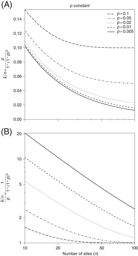
. But we generally do not have a reliable roster of species with k=0, meaning that the species really were present in a specified area at a particular time but were not found at any sampled sites. Therefore our observed values of k are necessarily greater than zero and k/n is biased upward (Fig. 1). (This situation is common in ecology, in part because so many species are rare [Fisher et al. Reference Fisher, Corbet and Williams1943; Preston Reference Preston1948; Rabinowitz Reference Rabinowitz1981], and is not merely a paleontologist’s headache reflecting the incompleteness of the fossil record.) Specifically, if p is a constant, the probability that k sites will be occupied, given that k is greater than zero, is equal to a conditional binomial:
 $${\rm B}'\left( {k;n,p} \right)=\left( {\matrix{ n \cr k \cr } } \right){{p^{k} \left( {1{\minus}p} \right)^{{n{\minus}k}} } \over {1{\minus}\left( {1{\minus}p} \right)^{n} }};$$
where the denominator is the probability that k>0, and the expected number of sites occupied per species is equal to np/[1−(1−p)
n
] (see Appendix). Therefore, the estimate
 $$\bar{k}/n$$
is higher than p by a factor of 1/[1−(1−p)
n
]. The bias resulting from this kind of data censoring was discussed by Haldane (Reference Haldane1932, Reference Haldane1938) and Fisher (Reference Fisher1936) in the context of estimating frequencies of genetic conditions in human populations (in which families with no instances of the condition may go unreported). Finney (Reference Finney1949) and Rider (Reference Rider1955) also discussed the more general problem of truncated binomial distributions where k>1, k>2, and so on.
Dependence of mean proportional occupancy (
 $$\bar{k}/n$$
) on occupancy probability (p) and number of sites (n), when p is constant and k>0. A, Mean occupancy. B, Ratio of mean occupancy to true occupancy probability. Bias inherent in
 $$\bar{k}/n$$
increases as p decreases and as n decreases.
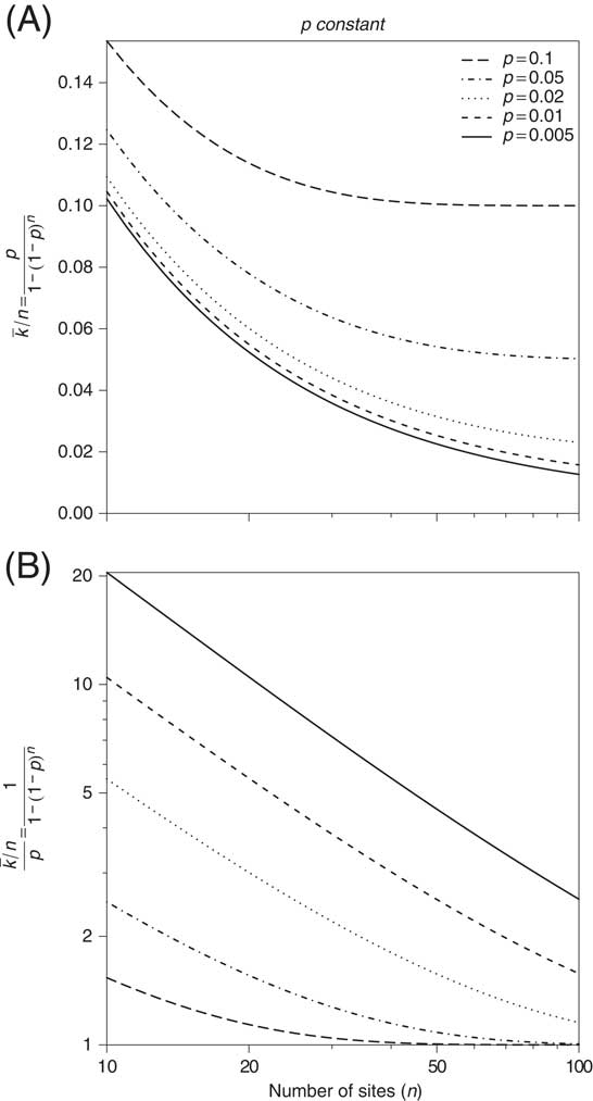
The bias caused by filtering cases where k=0 is exacerbated by variation in the number of sites sampled, n. As n becomes smaller, the difference between k/n and the underlying occupancy probability increases (Fig. 1), to the point where k/n=1 when n=1, regardless of the true occupancy probability. If, for instance, we wanted to construct a time series of average taxonomic occupancy to assess the extent to which genera tend to be more broadly distributed in the aftermaths of mass extinctions than during other times (Schubert and Bottjer Reference Schubert and Bottjer1995; Hallam and Wignall Reference Hallam and Wignall1997; Erwin Reference Erwin2001; Miller and Foote Reference Miller and Foote2003), the time series could potentially be strongly and inversely correlated with the number of sites per time interval.
Strictly speaking, the occupancy probability, p, is the joint probability that a species actually lived at a site and that it was detected. It is possible in principle to estimate detection probabilities separately given data on repeated surveys of the same sites within a time span sufficiently short that what lives where has not changed (MacKenzie et al. Reference MacKenzie, Nichols, Lachman, Droege, Royle and Langtimm2002, Reference MacKenzie, Nichols, Hines, Knutson and Franklin2003, Reference MacKenzie, Nichols, Royle, Pollock, Bailey and Hines2006; Royle and Nichols Reference Royle and Nichols2003; Dorazio et al. Reference Dorazio, Royle, Söderström and Glimskär2006). In contrast to these studies, I am assuming data in which we have but one sample, possibly aggregated over several collections, for each site. For simplicity I will continue to use occupancy probability as the probability that a species is found at a site; this is also referred to as incidence (e.g., Colwell et al. Reference Colwell, Chao, Gotelli, Lin, Mao, Chazdon and Longino2012; Chao et al. Reference Chao, Gotelli, Hsieh, Sander, Ma, Colwell and Ellison2014, Reference Chao, Hsieh, Chazdon, Colwell and Gotelli2015a).
Haldane and Fisher’s Solution
In the problem facing Haldane and Fisher, k
i
is the number of instances of a genetic condition in family i; n
i
is the size of family i; and S is the observed number of families. (Haldane and Fisher in fact used different notation.) For most of this discussion, I will assume that n, the number of potential sites, is the same for all species, but this assumption is not essential (Appendix). The maximum-likelihood solution used by Haldane and by Fisher depends only on
 $$\bar{k}$$
and n, and simply requires finding, by numerical methods, the value of p such that
 $$\bar{k}/n$$
is equal to p/[1 − (1 − p)
n
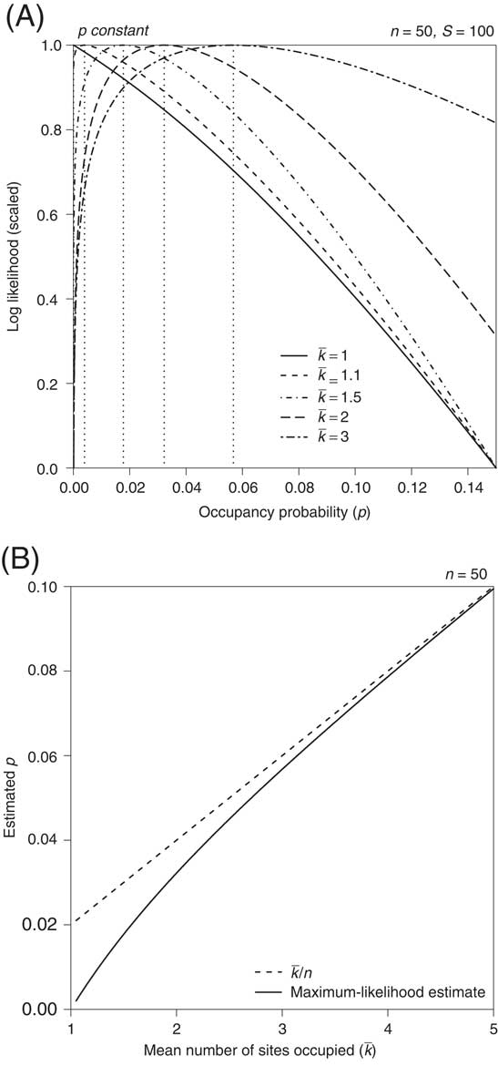
], but of course the solution is more tightly constrained as S increases. Figure 2A shows several examples of log-likelihood (support) functions; the values of p corresponding to the maxima are always less than
 $$\bar{k}/n$$
. Note that the case where
 $$\bar{k}=1$$
has no maximum-likelihood solution, as the support function has no peak. Thus, using the Haldane–Fisher approach, if all species are known from a single site, we cannot estimate the underlying occupancy probability. The proportional difference between
 $$\bar{k}/n$$
and the maximum-likelihood estimate,
 $$\hat{p}$$
, decreases as k increases (Fig. 2B), and it also decreases as n increases (Fig. 1B). This maximum-likelihood solution addresses both the fact that k is biased upward and that the magnitude of this bias depends on n. The Haldane–Fisher solution has the simplicity that the ratio of
 $$\hat{p}$$
to
 $$\bar{k}/n$$
is nearly constant for a given value of
 $$\bar{k}$$
; for example,
 $$\hat{p}$$
=0.168 when
 $$\bar{k}=2$$
and n=10, and
 $$\hat{p}=0.0160$$
when
 $$\bar{k}=2$$
and n=100.
Haldane–Fisher maximum-likelihood estimate of p when p is constant and k>0. A, Log-likelihood curves illustrated with n=50 and number of species, S=100, and selected values of
 $$\bar{k}$$
. Curves are scaled to have a maximum of unity. Vertical dotted lines indicate the maximum-likelihood estimates, which are always lower than
 $$ \bar{k}/n$$
; note that the curve for
 $$ \bar{k}=1$$
has no peak. B, Maximum-likelihood estimate of p as a function of
 $$\bar{k}$$
. Although width of support curves depends on S, the estimate of p depends only on
 $$\bar{k}$$
and n.
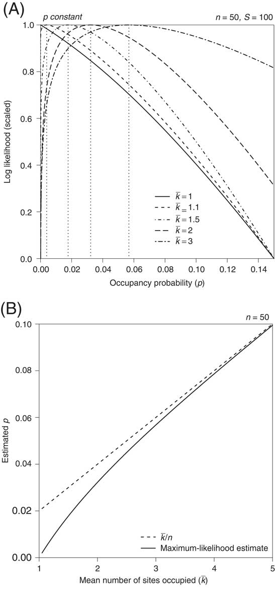
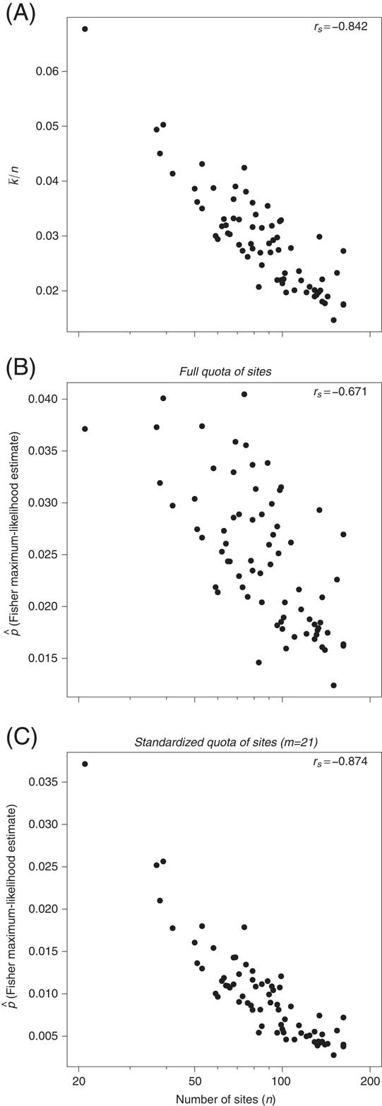
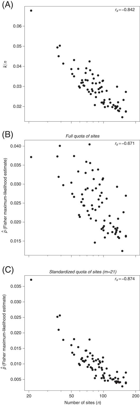
Figure 3 shows results of applying the Haldane–Fisher solution to occupancy data on Phanerozoic marine animal genera extracted from the Paleobiology Database (paleobiodb.org). See Foote et al. (Reference Foote, Ritterbush and Miller2016) for details on the data. Each point represents a stage, and the sites are equal-area map cells of approximately 2×10⁵ km2. The value of n for each stage is taken as the number of cells that contain any data in that stage, that is, the maximum value that k could take on. The average proportional occupancy,
 $$\bar{k}/n$$
, depends strongly on n (Fig. 3A), as we would expect from Figure 1. The maximum-likelihood solution reduces this dependency only somewhat (Fig. 3B). Sampling standardization might seem like a promising approach, but in fact it does not circumvent the number-of-sites bias. If, for example, we randomly draw data from the same number of cells for each stage and use the Haldane–Fisher solution, the correlation between the estimated occupancy probability and the original number of cells is just as strong as that between
 $$\bar{k}/n$$
and the number of cells (Fig. 3C). Why should that be?
Analysis of data on marine animal genera, where k is the number of equal-area cells (2×10⁵ km2) occupied by a genus and n is the total number of cells with any data in a given stage. Each point denotes a single stage. A, Mean raw proportional occupancy,
 $$\bar{k}/n$$
. B, Haldane–Fisher maximum-likelihood estimate of occupancy probability, assuming p is constant for each stage. C, Maximum-likelihood estimate of p, assuming p is constant, when data are first subsampled, so each stage is represented by the same number of randomly chosen cells (equal to n = 21, the minimum among all stages), based on the mean of 100 replicates. Bias in
 $$\bar{k}/n$$
is expected even if p is constant. Bias in maximum-likelihood estimate is interpreted in part to reflect the fact that p is in fact a probability distribution for each stage and that higher values of p are sampled preferentially at lower values of n.
As Haldane and Fisher were aware, their solution applies when p is constant, which was appropriate in their application, because they were testing for consistency with specific, fixed genetic ratios. Their solution is not strictly applicable when p varies, because the basis of the solution lies in modifying binomial sampling probabilities by the probability that k>0, which is equal to 1 − (1 − p)
n
if p is constant, but which is not in general equal to
 $$1{\minus}(1{\minus}\bar{p})^{n} $$
when p varies among species and has mean
 $$\bar{p}$$
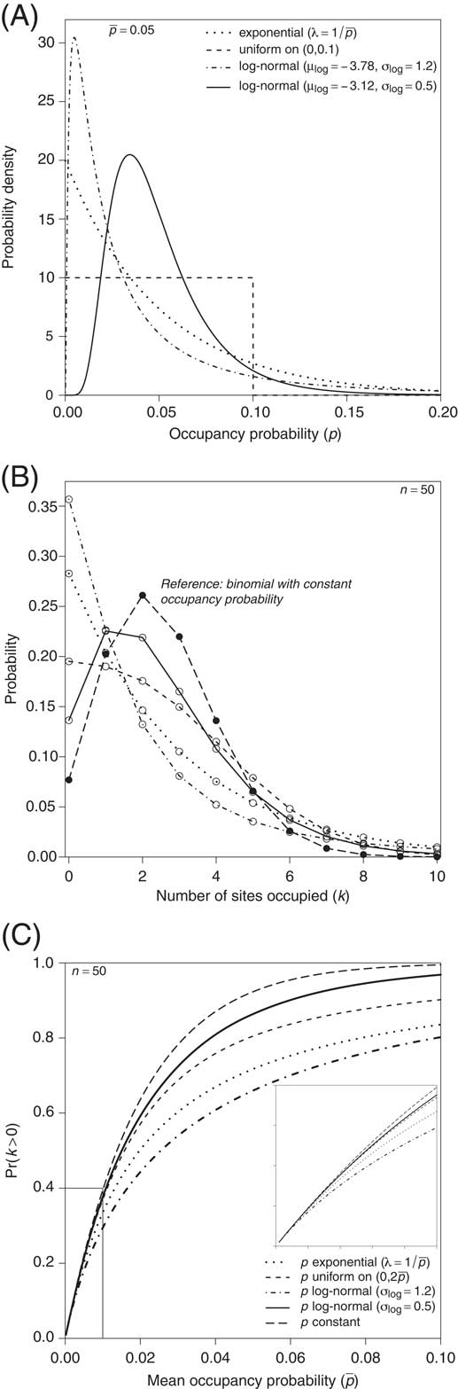
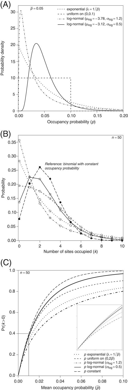
(Appendix). For a given distribution of occupancy probabilities, as we sample fewer sites we preferentially sample the species with higher occupancy probabilities, that is, the more common species. The shape of the distribution is crucial, because the probability that k>0 depends on it. Figure 4A shows examples for four different distributions that all have the same mean occupancy probability,
 $$\bar{p}$$
. Although the mean is the same, the probability that k>0 varies substantially and is lower in each instance than it would be if p were constant (Fig. 4B,C). The Haldane–Fisher maximum-likelihood approach can easily be modified to encompass variability in p if we can either assume the distribution of p or fit it to the data. The essence lies in determining the probability that k out of n sites will be occupied for a given value of p and integrating this over the entire distribution of p (Appendix).
Examples of variable distributions of occupancy probability. A, Four distributions that all have the same mean value,
 $$\bar{p}=0.05$$
. B, Corresponding probability distributions of occupancy, k, with binomial distribution (i.e., constant p) for comparison. C, Probability that k>0 as a function of
 $$\bar{p}$$
and shape of distribution (inset shows detail of highlighted area). Probability that k>0 is generally lower for variable distributions than for constant p, especially if the distribution is right skewed.
Modeling and Fitting the Distribution of Occupancy Probabilities
I will illustrate the modeling of occupancy probabilities for the data on Phanerozoic marine animal genera using a log-normal distribution of p. This distribution has two parameters, μlog (the mean of the logarithm of p) and σlog (the standard deviation of the logarithm of p). Because the log-normal distribution allows for values up to +∞, we must modify it if we use it to model occupancy probabilities. I have therefore fitted a truncation point, p max, the maximum value that p can take on, as a third parameter. I will hereinafter refer to the resulting distribution as the “truncated log-normal.” Note that this is a different usage of a term that has been used to refer to left-truncated distributions of species abundance data, which are analogous to k rather than p (Preston Reference Preston1948; Slocomb et al. Reference Slocomb, Stauffer and Dickson1977; McGill Reference McGill2003).
When p is expressed on an arithmetic scale, the distribution is right skewed, just as occurrence and occupancy measures often are, but it also has a mode, which seems biologically realistic. If occupancy probability reflects geographic range, for instance, a distribution with peak probability at zero, such as the beta(α, β) distribution with α < 1 (Appendix), would imply that there are more species occupying a postage stamp–sized piece of real estate than those with some minimum viable range well above such a theoretical minimum. (Examples of distributions of k with a mode at k=1 include the log-series and Zipf [Buzas et al. Reference Buzas, Koch, Culver and Sohl1982; Wagner et al. Reference Wagner, Kosnik and Lidgard2006].) The log-normal also has some rationale for occupancy, insofar as such a distribution is expected to result as the product of many biological factors, such as geographic range, local abundance, niche breadth, and availability of suitable habitat, as well as aspects of sampling, such as human effort and, in the case of paleontology, availability of outcrop and intrinsic preservation potential. In a similar vein, Wagner and Marcot (Reference Wagner and Marcot2013) have demonstrated that a log-normal distribution tends to provide a good model for paleontological sampling rates. As noted above, these occupancy probabilities necessarily reflect the joint probability that a taxon in fact lived at a given site and that it was detected. The approach assumes that occupancy and detection probabilities are properties of species and overlooks the fact that these may vary among sites. I will return to this issue below.
Two points to bear in mind before proceeding: (1) The goal is to characterize and estimate the distribution of p (e.g., Fig. 4A) that underlies the distribution of k (e.g., Fig. 4B), not the distribution of k itself (cf. Buzas et al. Reference Buzas, Koch, Culver and Sohl1982). The shape of the distribution of k may resemble that of p, but clearly it need not do so. As an obvious example, if p is constant, k will have a binomial distribution. (2) As with the Haldane–Fisher approach, it will not be possible to estimate occupancy probability if all species are known from a single site.
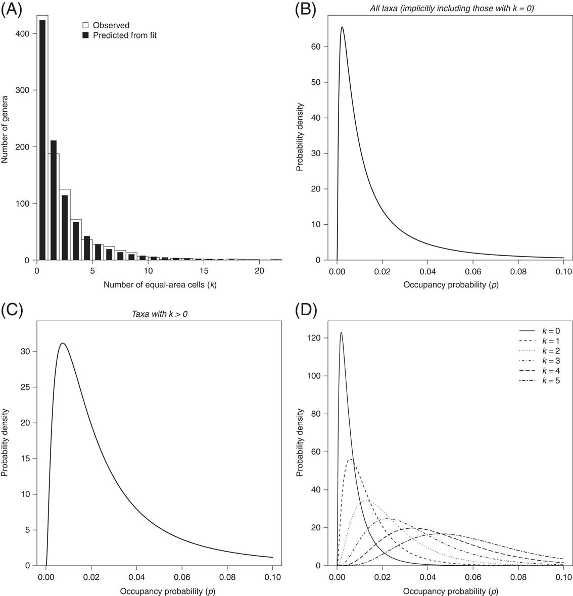
Figure 5A shows the frequency distribution of k for an arbitrarily chosen time interval, the Sandbian stage of the Ordovician. There are 69 cells (n), the maximum value of k is 22, the mean value of k is 2.69, and the mean value of k/n is 0.039. Also shown are the predicted values of k corresponding to the maximum-likelihood estimate of the distribution of p, which itself is given in Figure 5B. The mean of this distribution is 0.021, distinctly lower than
 $$\bar{k}/n$$
. This mean tacitly incorporates the occupancy probability of all genera, including unsampled genera, assuming they are all drawn from the same underlying distribution.
Example of fitting truncated log-normal distribution of occupancy probabilities to occupancy data for the Sandbian stage of the Late Ordovician. A, Observed frequency distribution of k and distribution predicted from best-fit log-normal distribution (B). C, Conditional probability distribution, corresponding to the best-fit curve in B, for the subset of genera with k>0. D, Conditional probability distributions for subsets of genera having specified values of k. Genera with higher values of k preferentially sample higher values of p, but even those with k=0 are inferred to represent a part of the probability distribution above zero.
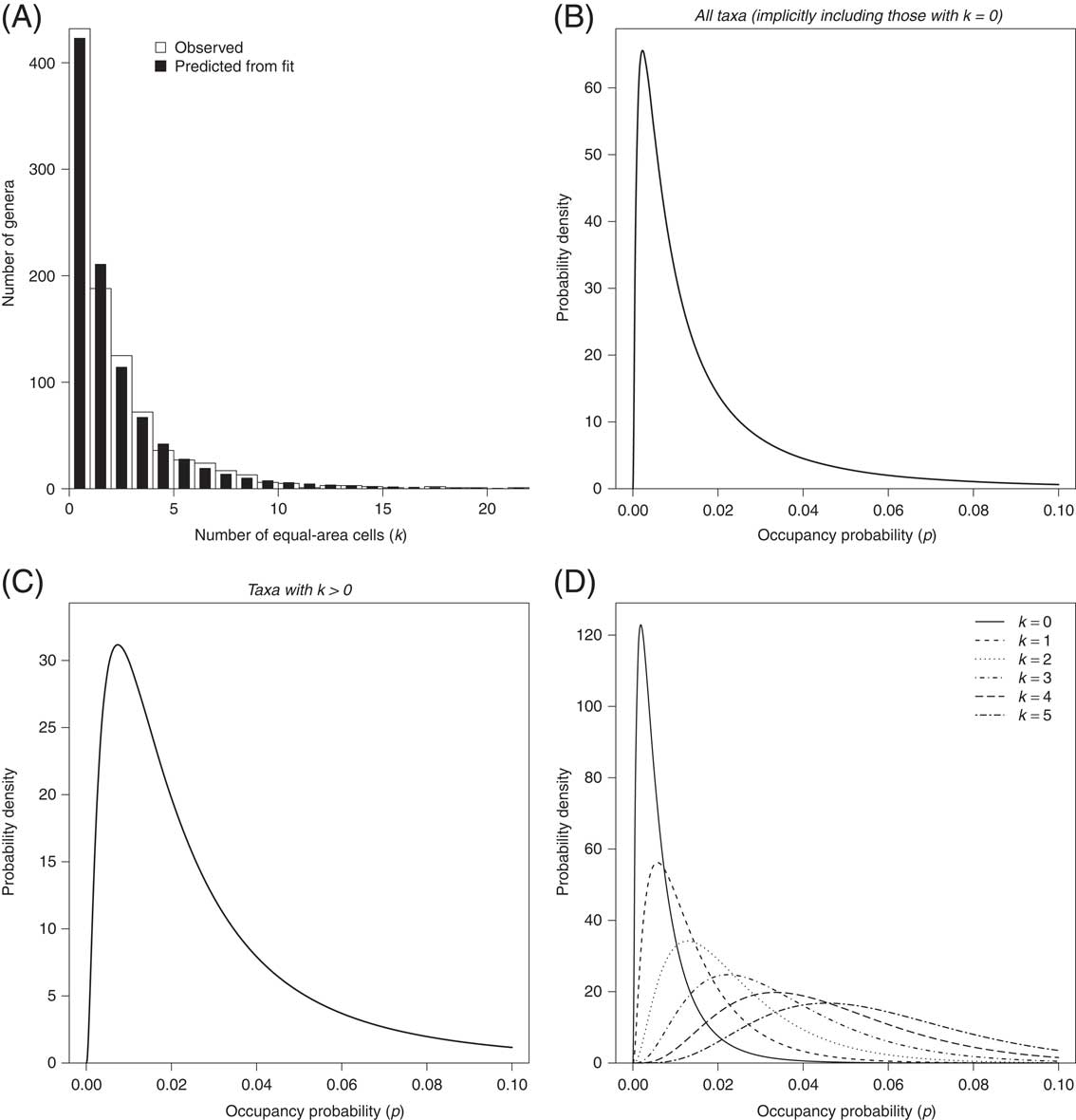
In addition to estimating the occupancy probability distribution of all taxa, we can estimate the part of the distribution corresponding to subsets of taxa with specified values of k. Those with k>0 preferentially sample higher values of p than those with k=0 (Fig. 5C,D), and those with progressively higher values of k reflect ever higher values of p (Fig. 5D). Even though the taxa with k>0 represent a biased subset of the entire probability distribution (Fig. 5C), fitting that distribution allows this bias to be circumvented.
Truncating the log-normal at p max is admittedly ad hoc and inelegant. John Alroy (personal communication 2016) has kindly suggested an alternative approach: to model the probabilities as a logit-normal distribution, in which logit(p), equal to log[p/(1 − p)], is normally distributed (Coull and Agresti Reference Coull and Agresti1999; Dorazio et al. Reference Dorazio, Royle, Söderström and Glimskär2006: p. 847). With p bounded between 0 and 1, logit(p) is unbounded from –∞ to ∞, no ad hoc truncation is necessary, and the distribution can be modeled with only two parameters, μlogit (the mean of the logit of p) and σlogit (the standard deviation of the logit of p). With the low values of p characteristic of the data analyzed here, the log-normal and logit-normal are rather similar. Moreover, by the time the truncation point is reached, the probability density has generally trailed off nearly to zero, so the fitted log-normal probability curve does not “drop off a cliff” at p max. The case in Figure 5 is typical. If for each stage we compare the probability density at p max to the maximum value of the density, the ratio of the two has a median ~1×10⁻⁴, and it is never higher than ~1×10⁻³. The median tail area to the right of p max is ~0.3%, and the maximum is ~2%.
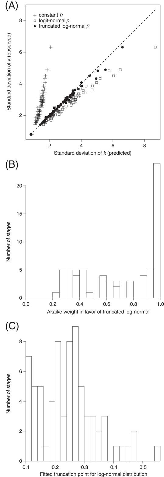
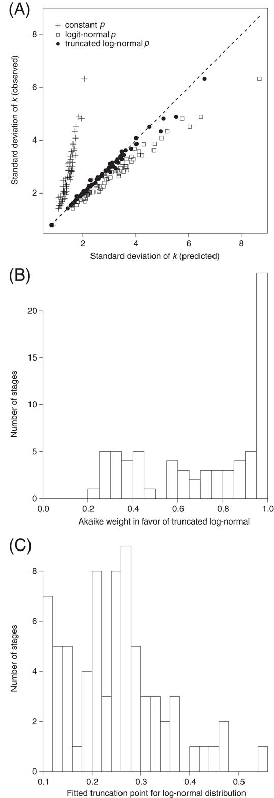
Figure 6 shows results of fitting three different distributions to each stage: (1) constant p; (2) truncated log-normal p; and (3) logit-normal p. Figure 6A compares the predicted and observed standard deviation of k. If we assume p is constant for each stage and use the Haldane–Fisher approach to estimate it, the predicted variance in k is substantially lower than what is observed. If we fit a logit-normal, the predicted variance is too high. This is because most genera have observed occupancy values, k, far to the left of the theoretical maximum value of n, that is, their observed proportional occupancies, k/n, are far below 1.0. However, the logit-normal integrates all the way to p=1.0 (i.e., logit[p]=∞) and therefore predicts some high values of k that increase the expected variance. (Similar results [not shown] obtain if we fit a log-normal truncated at p=1.0.) If instead we fit a truncated log-normal, we accurately capture the observed variation in k. Calculating the sample size–corrected AIC for each model for each stage (Fig. 6B), we see that the Akaike weights generally favor the truncated log-normal (median weight 0.80 vs. 0.20 for the logit-normal and 0.0 for the constant-p model) and that the median truncation point is around 0.25 (Fig. 6C).
Alternative models for fitting Phanerozoic occupancy data. A, Observed standard deviation of k compared with that predicted by model of: constant p (crosses); logit-normal p (open squares); and truncated log-normal p (closed circles). B, Akaike weights of truncated log-normal. C, Fitted truncation points. Truncated log-normal distribution is overall the best model of these three.
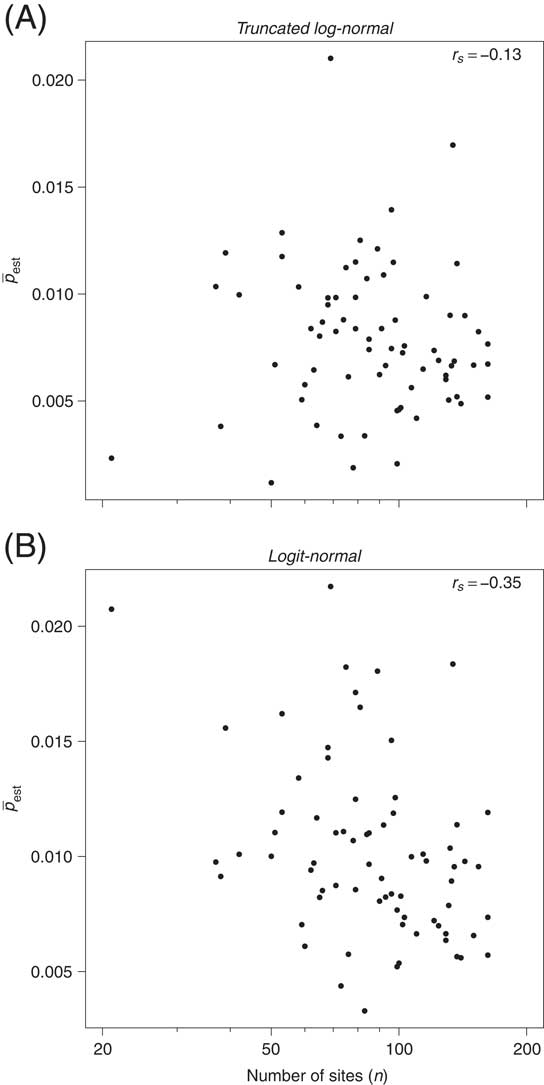
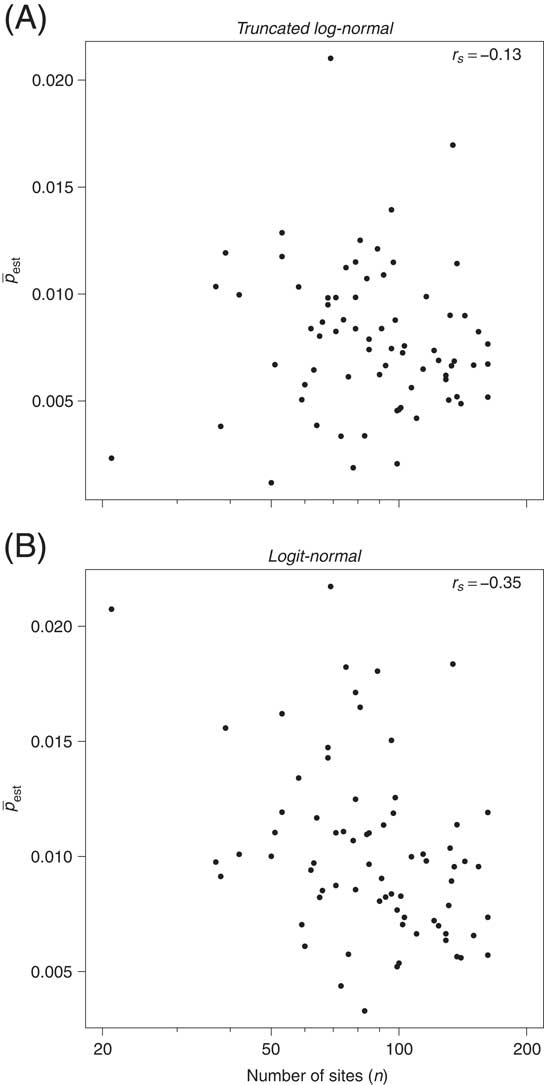
The agreement between predicted and observed variance in k is one sign that the truncated log-normal gives a reasonable fit to the data. Another sign is that the dependence between the number of cells, n, and the estimate of mean occupancy probability,
 $$\bar{p}$$
, essentially vanishes with this model (Spearman rank-order correlation coefficient: r
s
=−0.13, p > 0.25), whereas some bias, albeit weak, persists if we fit the logit-normal (r
s
=−0.35, p<0.01) (Fig. 7). The lack of correlation between n and
 $$\bar{p}$$
is to be expected if the data conform to the modeled form of the distribution, because n is explicitly taken into account in the likelihood function (Appendix).
Number of sites per stage versus estimated mean occupancy probability. A, Truncated log-normal. B, Logit-normal. Correlation between n and
 $$\bar{p}$$
is negligible for the log-normal and significant though weak for the logit-normal.
Whether to prefer the logit-normal or the truncated log-normal is somewhat a question of truth versus beauty. For aesthetics the logit-normal takes the prize, but given the data considered here, the truncated log-normal generally fits better, enough so to justify the extra parameter. I will therefore stick with the truncated log-normal for the rest of this paper. However, there is no obvious reason to suppose that it is preferable in general; the logit-normal, as well as other distributions, should certainly be considered in future work.
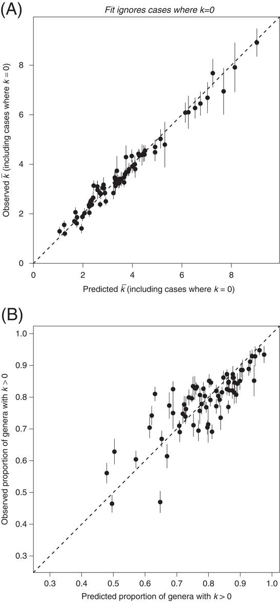
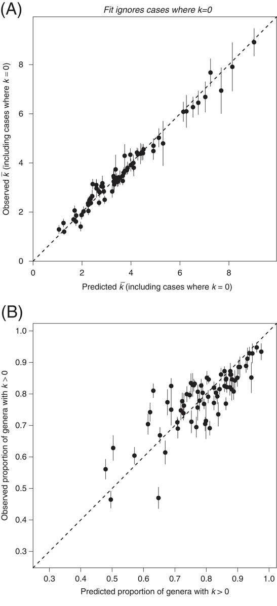
Another test of the truncated log-normal model is to use it to predict observations that were not involved in estimating the distribution. The distribution of p predicts the proportion of taxa with k=0, but—bearing in mind that what we mean by k=0 is that we know the taxon existed but it was not found at any sites—this prediction is not generally testable directly. One exception involves the subset of genera present in the stages immediately before and immediately after the stage in question, the three-timers and part-timers of Alroy (Alroy Reference Alroy, Aberhan, Bottjer, Foote, Fürsich, Harries, Hendy, Holland, Ivany, Kiessling, Kosnik, Marshall, McGowan, Miller, Olszewski, Patzkowsky, Peters, Villier, Wagner, Bonuso, Borkow, Brenneis, Clapham, Fall, Ferguson, Hanson, Krug, Layou, Leckey, Nürnberg, Powers, Sessa, Simpson, Tomašových and Visaggi2008; Alroy et al. Reference Alroy, Aberhan, Bottjer, Foote, Fürsich, Harries, Hendy, Holland, Ivany, Kiessling, Kosnik, Marshall, McGowan, Miller, Olszewski, Patzkowsky, Peters, Villier, Wagner, Bonuso, Borkow, Brenneis, Clapham, Fall, Ferguson, Hanson, Krug, Layou, Leckey, Nürnberg, Powers, Sessa, Simpson, Tomašových and Visaggi2008). We know these were extant during the stage and therefore know which ones have k=0 (the part-timers) and which have k>0 (the three-timers). For each stage, I fitted a distribution only to these through-ranging genera, including only those with k>0. I then used the fitted distribution to predict the mean value of k, including k=0; this mean correlates well with the observed value (Fig. 8A). The predicted proportion of genera with k>0 also provides a reasonable estimate (Fig. 8B).
Predictions involving genera with k=0 based on fit to genera with k>0. Only genera sampled in stages both immediately before and immediately after the stage in question are included. Each point is a stage; error bars are ±1 SE, based on bootstrap resampling of raw data (A) or binomial standard error (B). A, Mean occupancy. B, Proportion of genera with k>0. Predicted and observed values are well correlated.
Although the truncated log-normal may not be perfect, it is credible enough to consider applying it to some real occupancy problems. I will present a few examples showing how occupancy patterns are modified by the bias-correction approach. I will not interpret these biologically in any great detail.
A Few Applications
Permo-Triassic Distributions
Some genera and species are observed to be exceptionally widespread in the aftermaths of mass extinctions, particularly the end-Permian event (Schubert and Bottjer Reference Schubert and Bottjer1995; Brayard et al. Reference Brayard, Bucher, Escarguel, Fluteau, Bourquin and Galfetti2006: Figs. 7–8), but does this phenomenon reflect just a few genera or clades (Chen et al. Reference Chen, Kaiho and George2005), or is it general enough to influence average occupancy of the global fauna as a whole? Raw occupancy, measured as
 $$\bar{k}/n$$
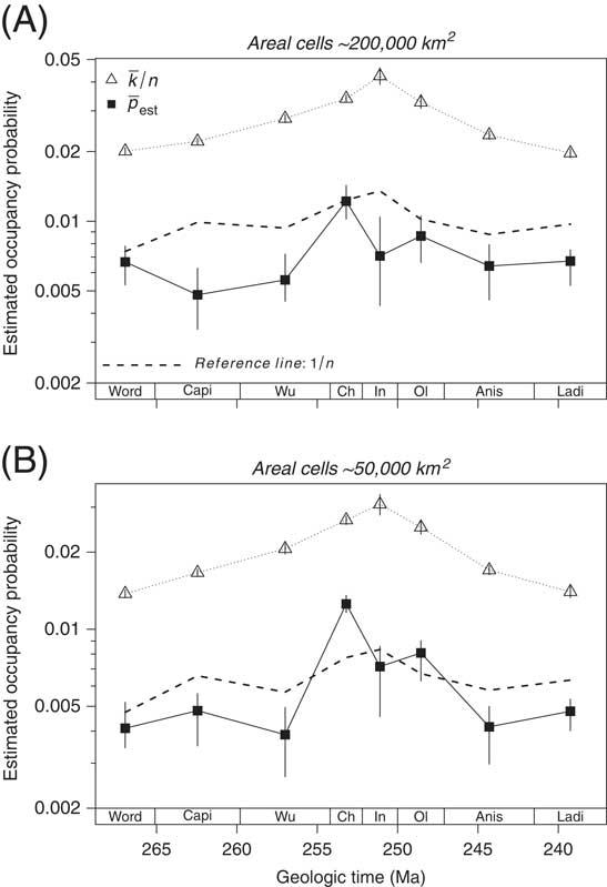
, steadily increases from the Guadalupian into the Triassic, hitting a peak in the earliest Triassic (Induan) and then declining into the Middle Triassic (Fig. 9A). However, the rise and fall, as well as the Induan peak, are precisely what we would expect from a corresponding decrease and increase in the number of sites, n (dashed line in Fig. 9A). For each stage, the occupancy data were fit with a truncated log-normal, from which the mean occupancy probability,
 $$\bar{p}$$
, was calculated. In addition, we want to know the uncertainty in the estimate of
 $$\bar{p}$$
that derives from the fitted parameters, given the sample of data at hand. One general approach to such problems is resampling (Efron and Tibshirani Reference Efron and Tibshirani1993). I applied the fitting procedure to 100 bootstrap samples of the data in each stage, resampling the values of k with replacement. Thus, the observed number of genera (S) and sites (n) remain fixed; it is simply the distribution of k that varies among bootstrap samples. (I obtain similar results [not shown] using the asymptotic estimate of the covariance matrix of the parameters, equal to the inverse of the observed information matrix [i.e., minus the matrix of second-order partial derivatives of the log-likelihood function, evaluated at the maximum-likelihood parameter estimates] [Edwards Reference Edwards1991]; drawing random trios of [μlog, σlog, p
max] from the corresponding multivariate normal distribution; and calculating the value of
 $$\bar{p}$$
for each parameter trio, thereby effecting a parametric bootstrap of
 $$\bar{p}$$
.)
Raw mean occupancy and estimated mean occupancy probability for the middle Permian through Middle Triassic. Timescale in this and the following figure is from Gradstein et al. (Reference Gradstein, Ogg, Schmitz and Ogg2012). A, Larger equal-area cells, corresponding to those used in the foregoing analyses. B, Smaller cells. Estimates of
 $$\bar{p}$$
are medians of 100 bootstrap replicates; error bars are interquartile ranges. Raw occupancy data suggest a steady rise and fall with an Induan peak, but this pattern parallels a fall and rise in the number of sites. Bias correction suggests peak occupancy in the Changhsingian but still relatively high values in the Induan and Olenekian if we consider a finer partitioning of the globe.
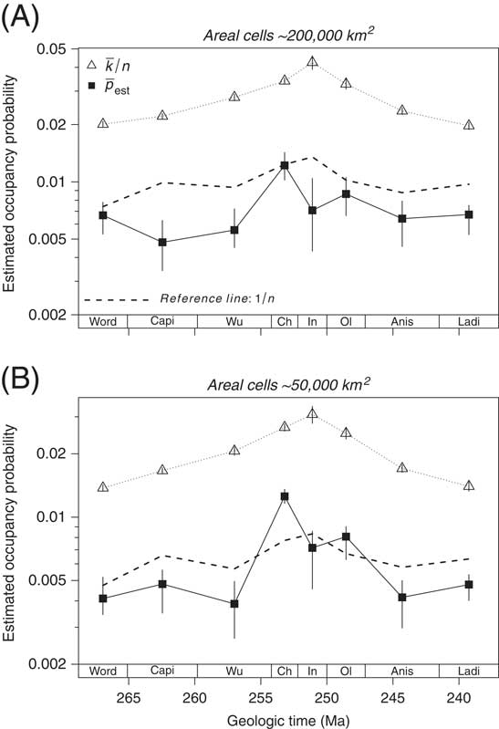
Because some of the bootstrap distributions are skewed, the results are presented as the median value of
 $$\bar{p}$$
and the interquartile range. It appears that occupancy is maximal in the latest Permian (Changhsingian) rather than the Induan; that the peak in the Induan may partly be an artifact of a low value of n; and that occupancy through the Early and Middle Triassic may be more constant than suggested by the raw data. However, the uncertainty in the Induan occupancy estimate is large, so these inferences must be regarded with caution. The increase in occupancy from the Guadalupian to the Lopingian, in both the raw data and in the bias-corrected estimate, agrees with raw, area-based geographic-range data reported by Clapham et al. (Reference Clapham, Shen and Bottjer2009: Fig. 10).
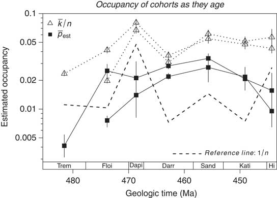
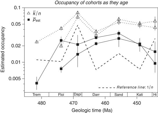
Raw mean occupancy and estimated mean occupancy probability for Early Ordovician cohorts. Estimates of
 $$\bar{p}$$
as in Fig. 9. Raw occupancy data suggest a peak in the Dapingian and stable values through the Late Ordovician. Bias correction suggests the Dapingian peak is an artifact of a low number of sites and an actual Hirnantian contraction is masked in raw proportional occupancy by a low site count in that stage as well.
In any study of occupancy, it is worth exploring sensitivity of results to the choice of what constitutes a site. In the Permian example, we get a slightly different view if we use smaller equal-area cells (Fig. 9B). The bias-corrected occupancy history suggests that, even though the peak is still in the Changhsingian, occupancy was also higher in the Early Triassic than during most of the focal interval, a pattern that is not quite so clear in the analysis using coarser spatial resolution.
Age and Area
In a pioneering study, Miller (Reference Miller1997) analyzed occurrence data on Ordovician marine animal genera and found that, as a whole, they tended to occur on more paleocontinents later in time, and that, during the Late Ordovician, the more widespread genera tended to be older. These results supported Willis’s (Reference Willis1926) age-and-area hypothesis. Figure 10 presents a complementary approach to this question, tracking occupancy of Early Ordovician (Tremadoc and Floian) cohorts as they age. Each point in this figure represents the occupancy of the genera that originated in one of these two stages and that were still extant and sampled during the stage in question, whether their stage of first appearance or a subsequent stage. As in Figure 9, distributions are fitted to each subset of data, and corresponding occupancy probabilities are represented by the median and interquartile range of a distribution of bootstrap estimates of
 $$\bar{p}$$
.
The raw occupancy measures suggest expansion of the cohorts; peak occupancy during the Dapingian stage; and relatively stable occupancy during the Late Ordovician (Sandbian–Hirnantian). However, the low cell counts in the Dapingian and Hirnantian, indicated by the peaks in 1/n, suggest that some aspects of these patterns may be suspect. The bias-corrected occupancy estimates indicate an expansion, consistent with the age-and-area model; absence of a peak in the Dapingian; and a decline in occupancy from the Sandbian through Hirnantian. This last feature contrasts with a Hirnantian expansion in geographic range documented by Darroch and Wagner (Reference Darroch and Wagner2015) using an area- rather than occupancy-based measure of genus extent.
Waxing and Waning
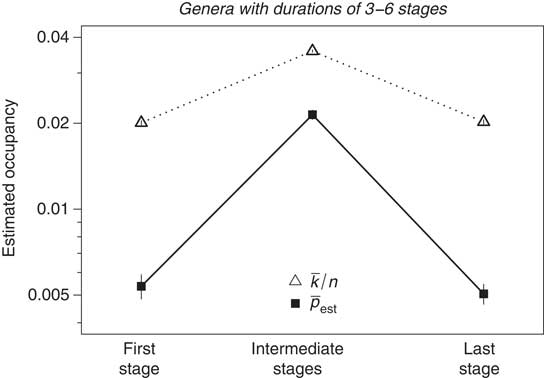
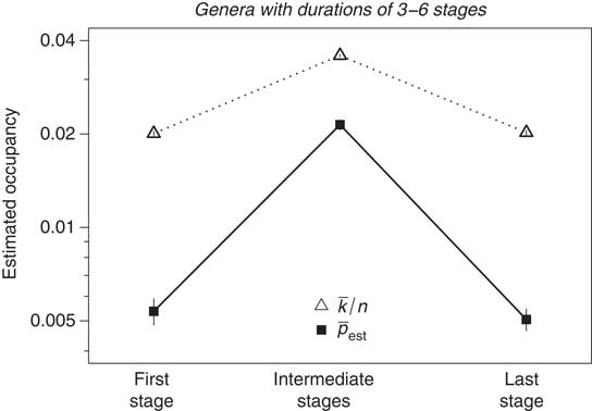
Several recent studies have sought to interpret aggregate occupancy histories of species and genera, irrespective of when they actually lived (e.g., Foote Reference Foote2007; Foote et al. Reference Foote, Crampton, Beu, Marshall, Cooper, Maxwell and Matcham2007; Liow and Stenseth Reference Liow and Stenseth2007). This approach would be expected to average out the biases caused by temporal variation in the number of sites. However, the fact that taxa early and late in their durations tend to be more restricted, as demonstrated by these studies, suggests that their lower occupancy probabilities would cause the raw value of k/n to exaggerate occupancy probability more during the intervals of first and last appearance than during intervening intervals (Fig. 1). To explore this possibility, I have aggregated data for all genera with stratigraphic ranges between three and six stages, inclusive; longer ranges that were omitted account for about 15% of the genera. I then estimated occupancy probability separately for the stage of first appearance, the stage of last appearance, and all intermediate stages combined, including only those genera actually sampled. (Because n varies among stages, these estimates use the likelihood function of eq. A8.) As expected, the pattern in bias-corrected estimates of occupancy agrees with that in the raw values of
 $$\bar{k}/n$$
insofar as both measures are lower during first and last stages (Fig. 11). However, the bias correction implies a much more dramatic pattern of expansion and contraction, with occupancy in intermediate stages about four times higher than in first and last stages, versus an 80% difference in
 $$\bar{k}/n$$
. The stronger bias in the first and last stages reflects both the lower values of
 $$\bar{k}/n$$
and, presumably, the higher frequency of genera with k=0, although this last point cannot be tested directly.
Aggregated occupancy data for all genera with durations of three to six stages, comparing the first stage, the last stage, and all intermediate stages combined. Observed occupancy expressed as mean of k/n ± 1 binomial SE; estimates of
 $$\bar{p}$$
are the mean of 100 bootstrap replicates ± 1 SE. Expansion and contraction of genera are much more pronounced in the bias-corrected occupancy estimate than in raw data.
Comparison with Coverage-based Estimation
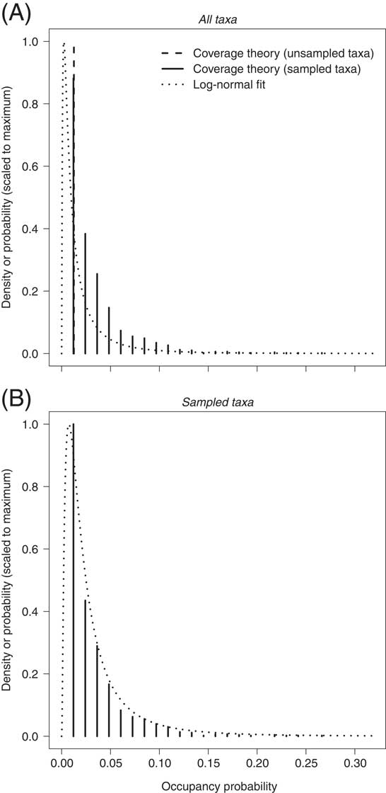
Coverage methods are based on estimating the proportion of species abundances or occurrences represented by a sample (Good Reference Good1953); the most notable paleontological application is Alroy’s (Reference Alroy2010a,Reference Alroyb) shareholder quorum subsampling algorithm. Chao et al. (Reference Chao, Hsieh, Chazdon, Colwell and Gotelli2015a: pp. 1198–1199) used a generalization of coverage theory to adjust k/n for individual species. They fit a two-parameter correction factor that, intuitively, assumes a declining exponential function, so that the larger the value of k, the smaller the correction. The parameters can be estimated, because coverage theory predicts the relationship between (1) the sum of occupancy probabilities of the sampled species, raised to an integral power defining the order of coverage; and (2) the complete suite of values of k/n (Chao et al. Reference Chao, Hsieh, Chazdon, Colwell and Gotelli2015a: eqs. D.6, D.7). The first-order coverage is the proportional sum of occupancy probabilities attributable to the sampled species. The complementary proportion represents the unsampled species, and the number of these unsampled species—actually a lower bound—can also be estimated (Chao Reference Chao1987). In this way, the true mean occupancy probability can be estimated for the sampled species, the unsampled species, and therefore the combination of the two. The estimation of coverage does not hinge on assuming any particular distribution. The coverage-estimated distribution of occupancy probabilities for the sampled species differs from that developed herein insofar as, with the coverage method, all sampled species with the same value of k are inferred to have the same, constant occupancy probability (cf. Fig. 5D); thus, the inferred probability distribution for sampled species is discrete. For the sake of illustration, Chao et al. (Reference Chao, Hsieh, Chazdon, Colwell and Gotelli2015a,Reference Chao, Hsieh, Chazdon, Colwell and Gotellib) assume that the unsampled species follow a geometric distribution, but this assumption is not crucial to the method and has no bearing on the estimated mean occupancy probability of sampled or unsampled species.
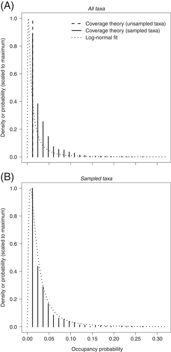
Figure 12 compares the occupancy probability distributions estimated with the two methods, applied to the data of Figure 5 (Chao et al. Reference Chao, Hsieh, Chazdon, Colwell and Gotelli2015b; Supplementary Data). The observed sum
 $$\sum k/n$$
is equal to 37.46. This provides an estimate of the sum of occupancy probabilities, including both sampled and unsampled taxa (Chao et al. Reference Chao, Hsieh, Chazdon, Colwell and Gotelli2015a: Appendix D); thus, the key issue is how that sum is divided among taxa and among how many taxa. There are 960 sampled genera. The coverage estimate implies that there are at least 490 unsampled genera, accounting for a summed occupancy probability of 6.18, and that the sampled genera account for a summed occupancy probability of 31.28. The estimated mean occupancy probability for sampled genera is therefore 0.0326 (31.28/960). The lower bound on the number of unsampled genera gives upper bounds for the mean occupancy probability equal to 0.0126 (6.18/490) for unsampled genera and 0.0258 (37.46/[960 + 490]) for all genera. The truncated log-normal fit yields estimates of mean occupancy probability equal to 0.0329 for sampled genera (eq. A14); 0.0073 for unsampled genera (eq. A12); and 0.0210 for all genera (eq. A10). Thus, the estimates of the summed occupancy probabilities accounted for by the sampled versus unsampled genera are quite similar with the two methods; where they differ is in the estimated or implied number of unsampled genera and therefore the mean occupancy probability of unsampled genera and of all genera.
Estimated distribution of occupancy probabilities for Sandbian genera (see Fig. 5), based on log-normal fit (dotted curve) and coverage-based analysis (bars). For sampled genera, height of bars is proportional to the number of genera with the corresponding occupancy probability. Unsampled genera are represented by a distribution of occupancy probabilities; in this instance they range only from 0.01260 to 0.01263 and so are depicted as a single, dashed bar in A. In this case, the coverage-estimated mean occupancy probability of unsampled genera is nearly the same as that of genera with k=1 (left-most solid bar), but this is not a general feature of the method. Other than one being discrete and the other continuous, the two methods yield similar distributions for sampled genera (B), whereas the log-normal fit yields lower mean probabilities for unsampled genera and therefore for all genera combined.
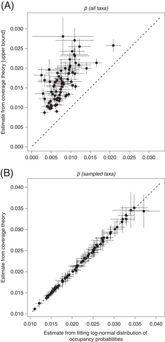
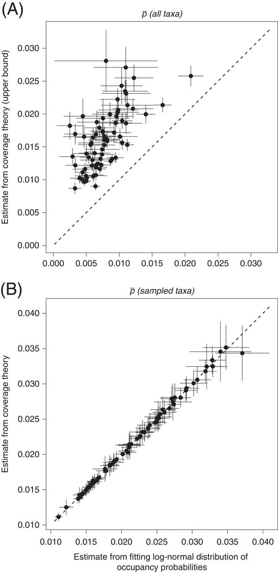
Carrying out the same calculations for all stages, the coverage-based estimate of mean occupancy probability for all taxa is consistently higher than the estimate based on the method of this paper (Fig. 13A), whereas the two estimates are nearly identical for sampled taxa (Fig. 13B). For these data, the standard error of the coverage-based estimates is generally smaller. Presumably this result reflects the fact that the method is distribution free.
Estimated mean occupancy probabilities, comparing log-normal fit (abscissa) to coverage-based estimate (ordinate). Each point is a stage. Error bars are ±1 SE, based on bootstrap resampling of genera within stages. Consistent with the results of Fig. 12, the two methods yield comparable occupancy probabilities for sampled taxa, whereas the log-normal fit yields lower estimates for unsampled taxa and for all taxa combined.
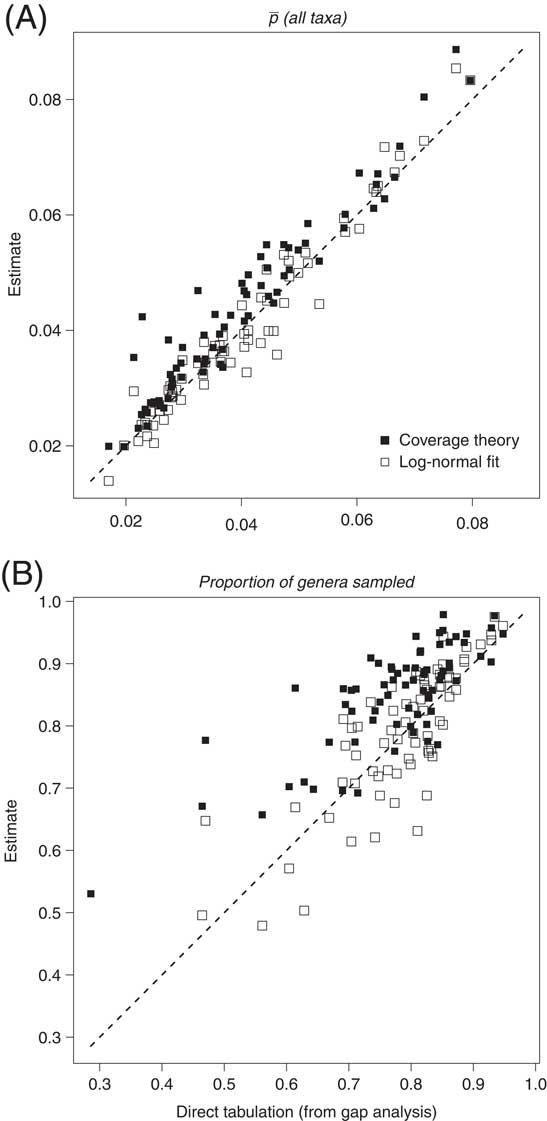
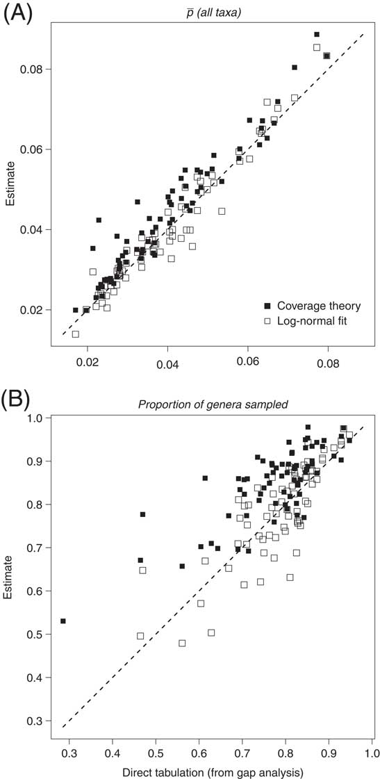
If for each stage we focus exclusively on genera that are known both immediately before and immediately after the stage (as in Fig. 8), we can use the sampled genera to produce occupancy estimates for all genera and compare these estimates to direct tabulations, because we know how many of the through-ranging genera have k=0. Figure 14 compares the two methods with respect to estimated mean occupancy for all genera (Fig. 14A) and the proportion of genera sampled at least once (Fig. 14B). The coverage-based estimates tend to overpredict these values, again an expected consequence of the estimation of a lower bound on the number of unsampled species.
Directly tabulated vs. estimated values of mean occupancy (A) and proportion of genera sampled (B), comparing the estimates from the log-normal fit (open squares) and the coverage method (closed squares). Abscissa shows direct tabulations of
 $$\bar{k}/n$$
(A), including cases where k=0, and the proportion of genera with k>0, i.e., the three-timer gap statistic (Alroy Reference Alroy2008; Alroy et al. Reference Alroy, Aberhan, Bottjer, Foote, Fürsich, Harries, Hendy, Holland, Ivany, Kiessling, Kosnik, Marshall, McGowan, Miller, Olszewski, Patzkowsky, Peters, Villier, Wagner, Bonuso, Borkow, Brenneis, Clapham, Fall, Ferguson, Hanson, Krug, Layou, Leckey, Nürnberg, Powers, Sessa, Simpson, Tomašových and Visaggi2008) (B). Estimated mean occupancy probabilities (A) and proportion of genera sampled (B) are based on analysis of genera sampled in the stages immediately before and immediately after the stage in question, and having k>0 during that stage, as in Fig. 8. The coverage-based estimates are generally higher than the direct tabulations and the estimates from the log-normal fit, suggesting that, for these data, the log-normal fit performs better at estimating the occupancy of unsampled taxa.
These last results suggest that the method developed herein may allow improved estimates of the mean occupancy probability of all taxa, sampled and unsampled, but it would be premature to generalize without further empirical and simulation studies and other approaches to estimating the number of unsampled taxa (Alroy Reference Alroy2010a,Reference Alroyb; Chao and Jost Reference Chao and Jost2012; Colwell et al. Reference Colwell, Chao, Gotelli, Lin, Mao, Chazdon and Longino2012; Chao et al. Reference Chao, Gotelli, Hsieh, Sander, Ma, Colwell and Ellison2014).
Discussion and Conclusions
The treatment so far has been confined to analyzing occupancy of distributions of taxa, generally coeval ones. Aggregate occupancy histories of noncoeval taxa were originally developed by superimposing point estimates for individual taxa in specific time periods (Foote Reference Foote2007; Foote et al. Reference Foote, Crampton, Beu, Marshall, Cooper, Maxwell and Matcham2007; Liow and Stenseth Reference Liow and Stenseth2007). As seen in Figure 11, such point values of k and n can be combined across taxa to develop a single, bias-corrected estimate of the distribution of occupancy probabilities. For some problems, however, we may still want a point estimate of the occupancy probability of a single taxon during one time interval. For example, Liow et al. (Reference Liow, Skaug, Ergon and Schweder2010) followed occupancy histories of individual species of planktonic microfossils. Although the results of Figure 11 suggest that the rise-and-fall pattern documented by Liow et al. (e.g., their Fig. 3) may be even steeper than in their raw proportional occupancy (k/n) data, it would take an unusual set of circumstances—with the number of sites falling and rising systematically through a species’ duration—for the basic occupancy pattern to be spurious. To take another example, I previously showed that when individual genera expand or contract in geographic range, these changes tend to coincide with expansions and contractions in the areal extent of their preferred habitat (Foote Reference Foote2014). In that particular case, the conclusions are probably robust, because compatible results were found using both k/n and k to measure geographic range, even though these measures respond in opposite ways to variation in n (Foote Reference Foote2014: Table A1). Nonetheless, it is worth considering how we might obtain point estimates that are free of the biases discussed here.
There are two obvious possibilities. First, we could assume that all species with the same value of k in a given time interval have the same, constant occupancy probability and apply the Haldane–Fisher method to each one, as in Figure 1B. But this approach seems undesirable, because the assumption of constant occupancy probability, even for just a subset of species, leads to inaccurate estimates of the mean probability, if in fact it varies, and because we cannot obtain an estimate for species with k=1, which often account for a plurality of data. Second, we could fit the distribution of occupancy probabilities to all species, extract the part of the distribution corresponding to taxa with any given value of k (including k=0) (Fig. 5D), and use the mean or median of this subdistribution as a point estimate.
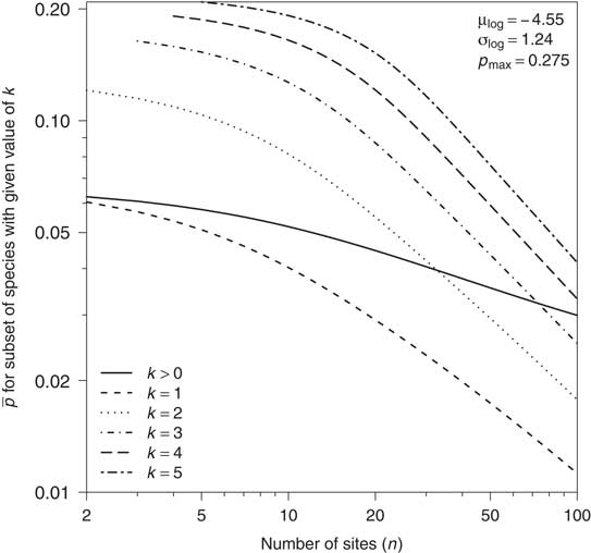
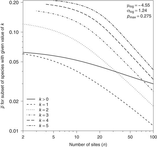
The latter approach is preferable, but it is worth remembering that the species actually sampled represent an upwardly biased subset of all species, and that, for a fixed underlying distribution of occupancy probabilities, the sampled species progressively represent the higher part of this distribution as the number of sampled sites decreases (Fig. 15). For example, using the distribution of Figure 5, sampled species have a mean occupancy probability of
 $$\bar{p}_{{k \, \gt\, 0}} =0.0356$$
if n=50 and 0.0301 if n=100 (eq. A14). This fact may seem like a nuisance, but point estimates for individual species should vary with n, because, all else being equal, species with a given value of k do in truth have a higher occupancy probability, on average, if n is lower.
Predicted mean occupancy probability for subsets of genera with selected values of k, as a function of number of sites, n. Curves are calibrated to the parameters fit to the Sandbian stage (see Fig. 5). Even if the underlying distribution of occupancy probabilities is fixed, the part of the distribution sampled by genera with a given value of k varies with n.
The situation with point estimates is analogous to that with the mean duration of a distribution of species versus the duration of a single species. Modeling the form of the true duration distribution and how it is affected by incomplete sampling allows an unbiased estimate of this distribution, even though observed stratigraphic ranges are truncated and some species are not recorded at all (Foote and Raup Reference Foote and Raup1996; Foote Reference Foote1997; Solow and Smith Reference Solow and Smith1997). However, individual species that are sampled represent an upwardly biased subset of the entire distribution (Foote and Raup Reference Foote and Raup1996: Fig. 2).
Extinction selectivity is another area in which revised occupancy estimates may make a difference. In particular, bias correction could affect the details of how much the odds of survival increase per unit increase in occupancy (Payne and Finnegan Reference Payne and Finnegan2007). Moreover, the prospect of estimating
 $$\bar{p}$$
for species that are known to exist but happen not to be sampled could provide an alternative to assigning arbitrary minimum values (Finnegan et al. Reference Finnegan, Payne and Wang2008) or ignoring them altogether (Foote and Miller Reference Foote and Miller2013).
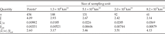
The Permo-Triassic example (Fig. 9) shows that some details of the temporal pattern of occupancy vary with the spatial resolution of a site or sampling unit. In the data analyzed herein, sampling is at a fine spatial scale, with the equal-area cells defined after the fact, so the number of sampled and unsampled genera is not affected by the resolution imposed. What about bias in the proportion of occupied cells? As resolution increases, that is, as the cell size decreases, both n and
 $$\bar{k}$$
increase, but n increases more rapidly so that
 $$ \bar{k}/n$$
decreases, as does estimated mean occupancy probability,
 $$\bar{p}$$
(Table 1). The increase in n would lead us to expect
 $$\bar{k}/n$$
to be less biased with higher resolution, whereas the decline in occupancy probability would lead us to expect the opposite. The former effect is evidently stronger, as the bias, that is, the ratio of
 $$\bar{k}/n$$
to
 $$\bar{p}$$
, decreases with increasing resolution.
Selected occupancy statistics, expressed as the median of all by-stage values, showing the effect of spatial resolution.

* All collections with the same geographic coordinates within a stage combined into a single sampling unit.
† Equal-area cells formed by dividing a Lambert cylindrical equal-area projection with the same number of latitudinal and longitudinal divisions: 200, 100, 50, and 25, respectively.
The aim of this paper has been to estimate an accurately scaled distribution of occupancy probabilities, from which one can derive means or other statistics, as well as point estimates for individual species. If the goal instead is simply to compare different data sets in terms of the relative magnitude of their mean occupancies, then sampling standardization of occupancy, based on a specified quota of sites or of coverage (Chao et al. Reference Chao, Gotelli, Hsieh, Sander, Ma, Colwell and Ellison2014), could potentially serve the purpose. One of the reasons for pursuing the approach of this paper, however, was the realization that with the data analyzed here, standardizing the number of sites, n, does not quite eliminate the dependence between n and
 $$\bar{k}/n$$
evident in the raw data. For example, if for each stage we sample n = 21 equal-area cells at random (the number corresponding to the smallest value for any stage)—replicating the subsampling and averaging the results—the original number of cells is still significantly correlated with the standardized mean occupancy (r
s
=−0.32, p < 0.01) (see also Fig. 3C). The circumstances under which rarefaction and related approaches eliminate the number-of-sites bias deserve further attention. One obvious potential limitation is that different occupancy distributions with the same value of
 $$\bar{p} $$
but different values of μlog and σlog are expected to yield different mean values of k (k>0), even if n is held fixed. For log-normal distributions typical of those estimated herein, decreasing μlog while increasing σlog, in such a way as to keep
 $$\bar{p}$$
constant, results in higher values of
 $$\bar{k}$$
(eq. A15) and lower values of S (eq. A7).
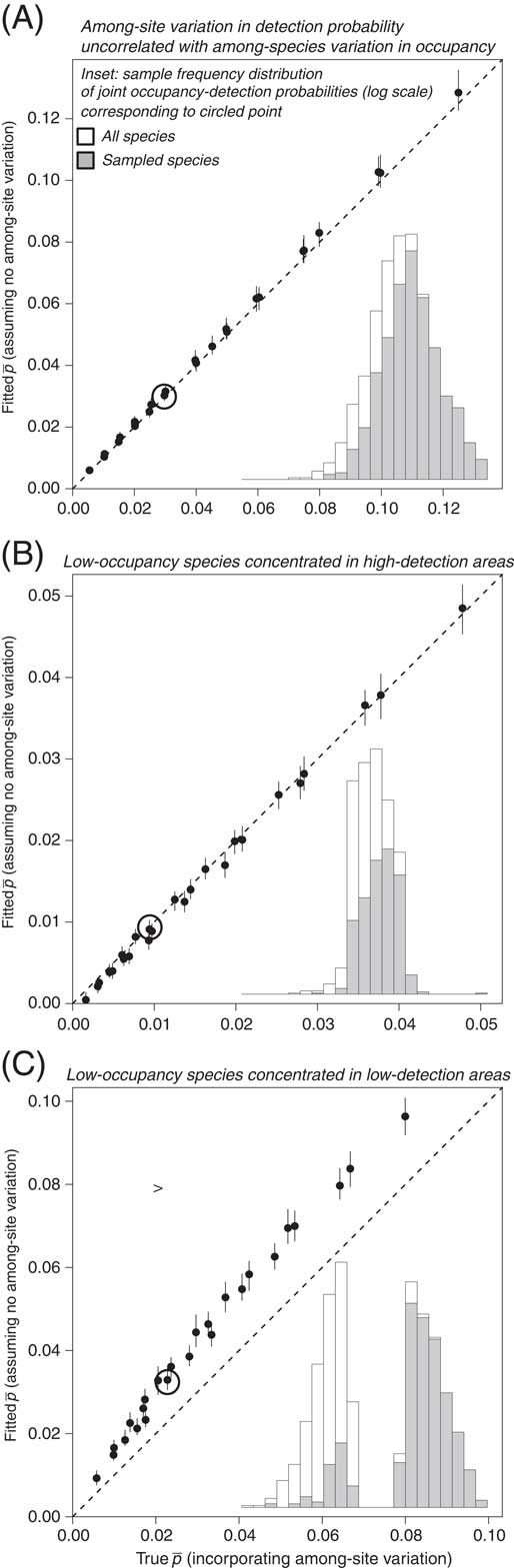
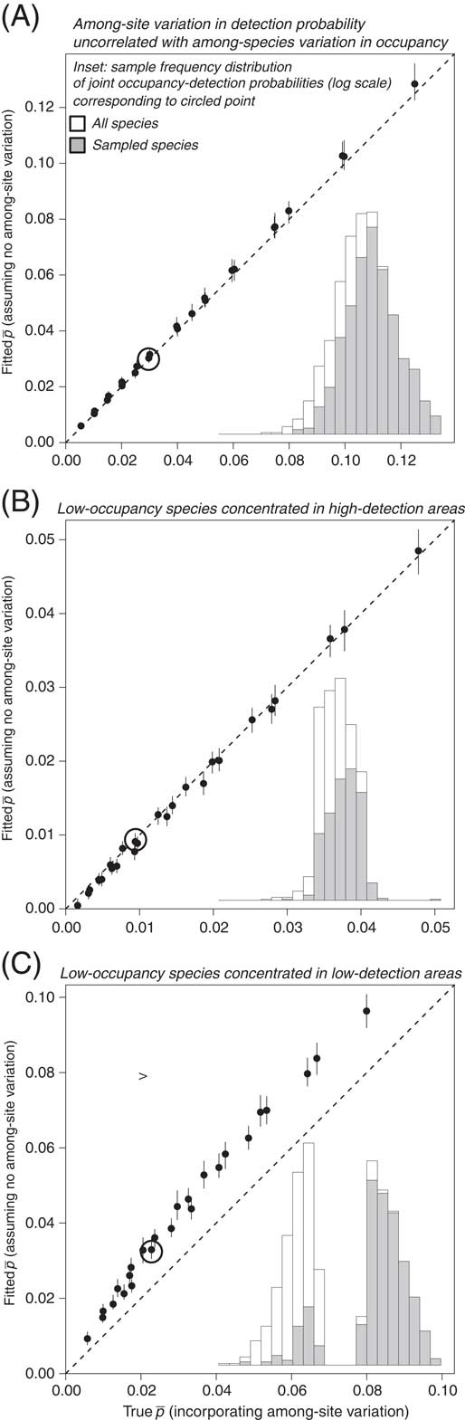
As noted earlier, the joint probability of occupancy and detection is treated as a property of species, without reference to among-site variation. To explore the possible effects of such variation, I carried out some simple simulations, in which each of S species is assigned an occupancy probability, p
sp,i
, and each of n sites is assigned a detection effect, p
site,j
, equal to the probability that a species truly occupying the site will be found. Thus, the probability, p
ij
, that species i will be observed at site j is equal to the product p
sp,i
×p
site,j
. The overall mean observation probability for species i, p
i
, is equal to
 $$ \mathop{\sum}\nolimits_{j=1}^n {p_{{ij}} / n} $$
; this is the quantity whose distribution we would like to estimate.
Values of p sp,i and p site,j were drawn at random from separate log-normal distributions. For simplicity, all distributions had p max=1.0, which was not treated as a fitted parameter, and all had σlog=1.0. Values of μlog were then assigned to yield five mean probabilities for species (0.05 through 0.25 in increments of 0.05) and five mean probabilities for sites (0.1 through 0.5 in increments of 0.1). All 25 combinations of species- and site-specific distributions were simulated, with 100 replicate simulations per combination. The true values of S and n were set to 1000 and 100, respectively, for each simulation; in general, fewer simulated species and sites actually ended up with nonzero occupancy. For each simulation, each value of p ij was compared to a uniform random number to determine whether the species i was found at site j. The value of k for each species was then tabulated as the number of sites at which the species was observed. The parameters were then estimated as with the empirical data; only nonzero values of k were included, and n was taken to be the number of sites with at least one species.
The simulated probabilities were treated according to three different regimens. (1) Species-specific occupancy probabilities were kept independent of site-specific detection probabilities, as in Dorazio et al. (Reference Dorazio, Royle, Söderström and Glimskär2006). (2) Species were ordered with respect to their occupancy probabilities, then divided at their median to form a low-occupancy group and a high-occupancy group. Similarly, sites were ordered and split into two “provinces” with low and high probabilities of detection. The joint occupancy-detection probabilities, p ij , were set to zero for low-occupancy species in low-detection sites and for high-occupancy species in high-detection sites. Thus, the simulated world was made to consist of one half with high-detection sites inhabited by low-occupancy species and another half with the opposite characteristics. (3) The treatment just described was modified so that low-occupancy species inhabit the half of the world with low-detection sites and likewise for high-occupancy species and high-detection sites.
If species- and site-specific properties are independent, then the mean of the joint occupancy-plus-detection probabilities (p i ) is recovered well (Fig. 16A). This stands to reason, as the product of two log-normal distributions is itself log-normal. If low-occupancy species are concentrated in high-occupancy sites, the low and high tendencies effectively offset each other, so the true mean is accurately estimated, even though the underlying distribution deviates from log-normal in the extent to which it is concentrated toward the center (Fig. 16B). If, by contrast, low-occupancy species are concentrated in low-detection sites, the distribution of p i is bimodal, the high-occupancy species evidently exert undue weight, and the mean is overestimated (Fig. 16C). It is unclear how common such situations may be in reality. One possible example would be tropical settings, for which the sampling of the fossil record is arguably comparatively poor (Jablonski et al. Reference Jablonski, Roy and Valentine2006, Reference Jablonski, Belanger, Berke, Huang, Krug, Roy, Tomasovych and Valentine2013), at least for the Cenozoic, and which have been interpreted by some as characterized by species with relatively narrow geographic ranges (Stevens Reference Stevens1989; see Willig et al. Reference Willig, Kaufman and Stevens2003 for discussion).
Simulation of among-site variation in detection probability superimposed on among-species variation in occupancy probability. Simulated data are analyzed without taking among-site variation into account. True and estimated probabilities reflect the mean of the joint probability of occupancy and detection. Points depict the median values across simulations; error bars show the interquartile range. A, Uncorrelated variation in occupancy and detection probabilities. B, Species with lower occupancy concentrated in sites with higher detection. C, Species with lower occupancy concentrated in sites with lower detection. (See text for details.) Insets show examples of simulated distributions corresponding to mean occupancy probability (
 $$\bar{p}_{{{\rm sp}}} $$
) of 0.15 and mean detection probability (
 $$\bar{p}_{{{\rm site}}} $$
) of 0.30 (circled points); the logarithmic horizontal scale is the same for all three insets and ranges from ~3×10⁻⁴ to ~3×10⁻¹. Note the comparatively peaked distribution in (B) and the bimodal distribution in (C). The largest estimation bias (C) occurs when low- and high-occupancy species are concentrated in low- and high-detection sites, respectively.
The approach outlined here can accommodate any density function with a simple substitution for f(p) (see the Appendix) and the calls to the R function dlnorm() and its associated parameters (see the Supplementary Data). The fit and performance of alternative distributions can then be compared as in Figures 6 and 7. In the case at hand, I initially worked with the beta distribution (Feller Reference Feller1971: p. 50) because of its great flexibility but found that in many instances, especially those with a very high proportion of genera occurring in just one cell, the shape of the likelihood surface did not allow a distinct maximum to be identified. See the Appendix for further discussion.
In summary, we have another way to circumvent the fact that observed occupancy is biased upward when we do not know how many taxa have k = 0 (i.e., they exist but do not occur in the data at hand) and that the magnitude of this bias is greater as the number of sites decreases. The approach depends on the ability to fit a distribution of occupancy probabilities that underlies the observed frequency distribution of occupancy counts and that implicitly includes unsampled as well as sampled taxa. In the data analyzed here, the truncated log-normal fits reasonably well for most stages, but other distributions should be explored for any given data set.
Acknowledgments
I am pleased to acknowledge many people who have contributed data to the Paleobiology Database. Major contributors for the data used herein include M. Aberhan, J. Alroy, D. Bottjer, M. Carrano, M. Clapham, S. Finnegan, F. Fürsich, S. Gouwy, N. Heim, A. Hendy, S. Holland, M. Hopkins, L. Ivany, D. Jablonski, W. Kiessling, M. Kosnik, B. Kröger, A. McGowan, T. Olszewski, P. Novack-Gottshall, J. Pálfy, M. Patzkowsky, A. Stigall, M. Uhen, L. Villier, and P. Wagner. I thank A. Chao, M. E. Clapham, J. S. Crampton, D. Jablonski, A. I. Miller, N. D. Pierrehumbert, F. M. Richter, K. Roy, G. J. Slater, P. D. Smits, A. Tomašových, M. Villarosa Garcia, and P. J. Wagner for discussion and advice; A Chao for assistance using the JADE code (Chao et al. Reference Chao, Hsieh, Chazdon, Colwell and Gotelli2015b); J. Alroy for suggesting the logit-normal distribution; and J. Alroy and J. L. Payne for helpful reviews of the manuscript. Supported by National Aeronautics and Space Administration, Exobiology (NNX10AQ44G). This is Paleobiology Database publication number 262.
Supplementary Material
Data available from the Dryad Digital Repository: http://dx.doi.org/10.5061/dryad.5sr24
Appendix: Estimating Occupancy Probabilities
The goal is to find the occupancy probability, p, that is, the probability that a species will occupy a site, if p is constant, or the probability distribution of p, f(p), if p varies. This distribution is distinct from the frequency distribution of the number of sites occupied, k. For example, if p is constant, k follows a binomial distribution. See Figure 4 for other examples. The number of sites is denoted n and the observed number of species S.
For a given n and p, the probability that exactly k sites will be occupied is given by the binomial:
 $${\rm B}\left( {k;n,p} \right)={\rm }\left( {\matrix{ n \cr k \cr } } \right)p^{k} (1{\minus}p)^{{n {\minus} k}} .$$
The probability that no sites will be occupied is equal to 1 − (1 − p) n . Therefore, the conditional probability that exactly k sites will be occupied, given that k>0, is given by
 $${\rm B}'\left( {k;n,p} \right)={{{\rm B}\left( {k;n,p} \right)} \over {1{\minus}\left( {1{\minus}p} \right)^{n} }}.$$
Therefore, if p is a constant, the likelihood of p, given a set of k i and n i (i=1, …, S) is proportional to
 $${\rm L}\left( {p;k,n} \right)=\prod\limits_{i=1}^S {{{p^{{k_{i} }} \left( {1{\minus}p} \right)^{{n_{{i }} {\minus} k_{i} }} } \over {1{\minus}\left( {1{\minus}p} \right)^{{n_{i} }} }}} ,$$
omitting the constant factors of
 $$\left( {\matrix{ {n_{i} } \cr {k_{i} } \cr } } \right). $$
If n is the same for all species, this simplifies to
 $${\rm L}\left( {p;k,n} \right)=\prod\limits_{k\,=\,1}^n {\left[ {{{p^{k} \left( {1{\minus}p} \right)^{{n {\minus} k}} } \over {1{\minus}\left( {1{\minus}p} \right)^{n} }}} \right]^{{N_{k} }} } ,$$
where N k is the number of species occupying exactly k sites. This likelihood is maximized by finding the value of p such that
 $$\bar{k}={{np} \over {1{\minus}\left( {1{\minus}p} \right)^{n} }} ,$$
where
 $$\bar{k}=\sum{k_i} /S$$
is the mean value of k (Fisher Reference Fisher1936: eq. 2). See Figures 1 and 2.
If p varies, then the probability that exactly k out of n sites will be occupied is obtained as the binomial probability for a given value of p, weighted by the probability density of p and integrated over all values of p:
 $${\rm P}\left( {k;n,\Theta } \right)={{\mathop{\int}\nolimits_0^{p_{{{\rm max}}} } {f\left( p \right){\rm B}\left( {k;n,p} \right)dp} } \over {\mathop{\int}\nolimits_0^{p_{{{\rm max}}} } {f\left( p \right)dp} }},$$
where Θ denotes the parameters that describe the density function f(p), and p max is the maximum value of p over which the probability density is integrated. This can be prescribed (e.g., as 1.0) or treated as a free parameter to be estimated. The denominator in the foregoing expression is necessary in cases in which we integrate over a range of values of p that does not sum to unity. For example, a log-normal distribution extends to +∞, but we cannot integrate p past 1.0. The probability that no sites will be occupied is P(0; n), the probability that at least one site will be occupied is 1 − P(0; n) (Fig. 4), and thus, the conditional probability that exactly k of n sites will be occupied, given that k>0, is given by
 $${\rm P}'\left( {k;n,\Theta } \right)={{{\rm P}\left( {k;n,\Theta } \right)} \over {1{\minus}{\rm P}\left( {0;n,\Theta } \right)}}.$$
In the case of the log-normal, the parameters are μlog, the mean of the logarithm of p; σlog, the standard deviation of the logarithm of p; and p max. The likelihood of Θ given a set of k i and n i , (i=1, …, S) is given by
 $${\rm L}\left( {\Theta ;k,n} \right)=\prod\limits_{i=1}^S {{\rm P}'\left( {\Theta ;k_{i} ,n_{i} } \right)} .$$
If n is the same for all species, this simplifies to
 $${\rm L}\left( {\Theta ;k,n} \right)=\prod\limits_{k=1}^n {\left[ {{\rm P}'\left( {\Theta ;k,n} \right)} \right]^{{N_{k} }} } ,$$
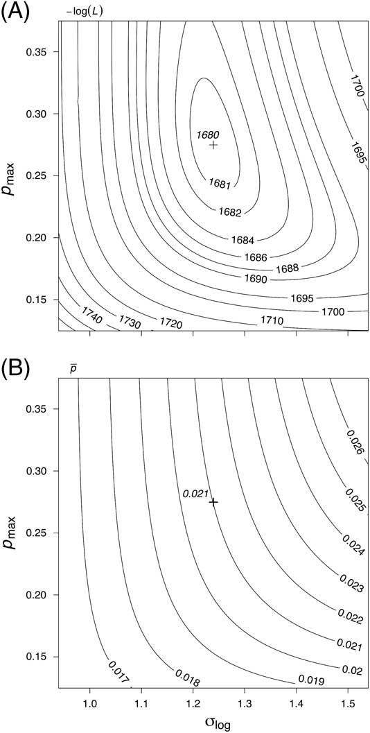
where N k is the number of species occupying exactly k sites. The estimates of Θ are found by numerically maximizing this likelihood function. Figures A1–A3 give an example.
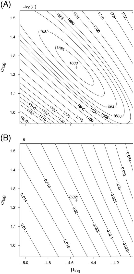
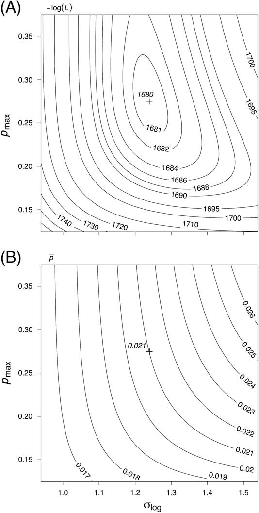
Contours of log-likelihood (A) and estimated mean occupancy probability (B) for the Sandbian example (Fig. 5), with p max held fixed at its maximum-likelihood estimate of 0.275 and with the position of the maximum-likelihood estimate of μlog and σlog indicated by the cross. For a log-normal distribution, the mean arithmetic occupancy probability depends on both the mean and standard deviation of the logarithms, being equal to exp(μlog+0.5σlog 2) if integrated out to +∞; this fact helps account for the general orientation of the contours.
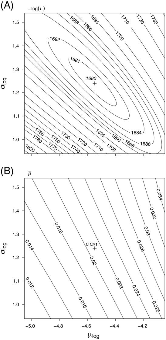
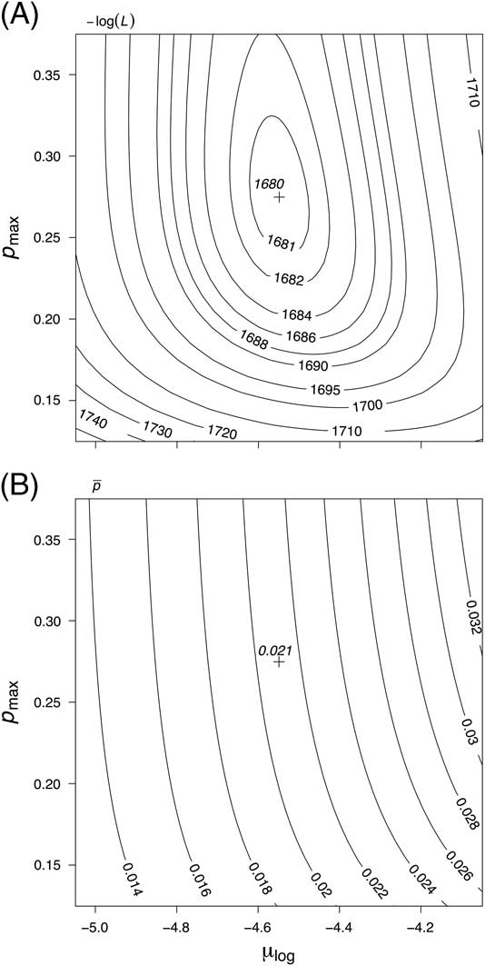
Contours as in Fig. A1, showing effect of μlog and p max with σlog held fixed at its maximum likelihood estimate of 1.24. Note the relatively small effect of p max over much of the range of values shown here, reflecting the fact that more than 95% of the probability distribution of p lies below 0.1 (Fig. 5).
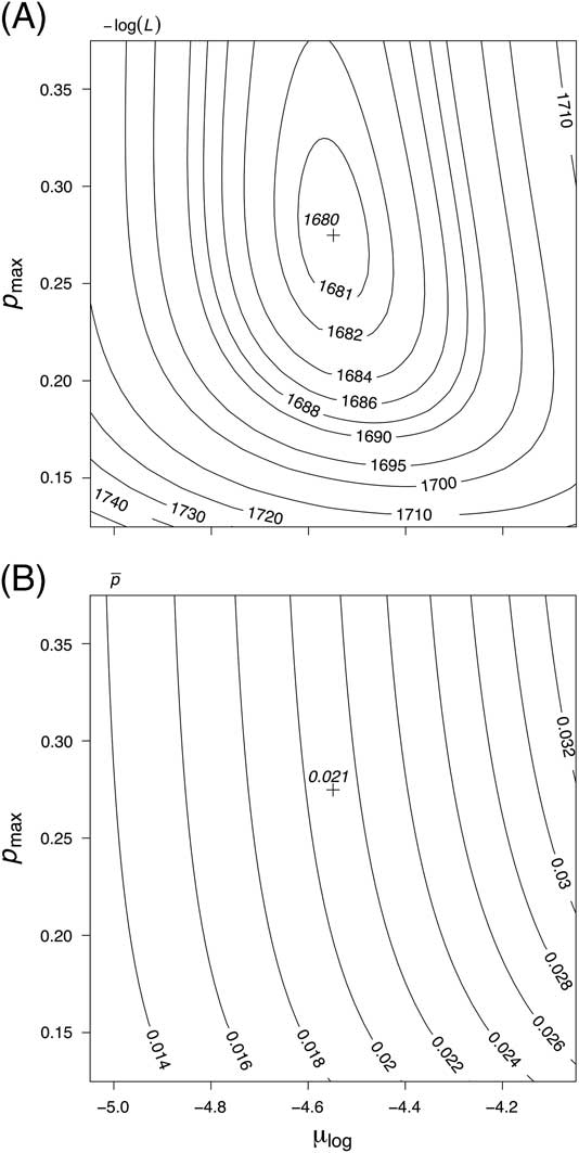
Contours as in Fig. A1, showing effect of σlog and p max with μlog held fixed at its maximum-likelihood estimate of −4.55.
Once we have the maximum-likelihood estimates of the parameters that describe f(p), the mean value of the probability distribution of p is given by
 $$\bar{p}={{\mathop{\int}\nolimits_0^{p_{{{\rm max}}} } {p \cdot f\left( p \right)dp} } \over {\mathop{\int}\nolimits_0^{p_{{\max }} } {f(p)dp} }}.$$
This implicitly includes species with k = 0 as well as those with k>0, that is, unsampled as well as sampled species.
For a specified value of k, the conditional density of p is obtained by Bayes’s theorem as the product of the density of p and the binomial probability of k given p, divided by the overall probability of k:
 $$f_{k} \left( p \right)={{f\left( p \right){\rm B}\left( {k;n,p} \right)} \over {{\rm P}\left( {k;n,\Theta } \right)}}$$
(Fig. 5D). From this we obtain the mean value of p for species with an occupancy of k as
 $$\bar{p}_{k} ={{\mathop{\int}\nolimits_0^{p_{{{\rm max}}} } {p \cdot f_{k} \left( p \right)dp} } \over {\mathop{\int}\nolimits_0^{p_{{{\rm max}}} } {f_{k} \left( p \right)dp} }}$$
(Fig. 15). Similarly, the conditional density of p given that k>0 is equal to
 $$f_{{k \,\gt \,0}} \left( p \right)={{f\left( p \right)\left[ {1{\minus}\,\left( {1\,{\minus}\,p} \right)^{n} } \right]} \over {1\,{\minus}\,{\rm P}\left( {0;n,\Theta } \right)}}$$
(Fig. 5C), and the mean value of p for all species with k>0 is equal to
 $$\bar{p}_{{k \,\gt \,0}} ={{\mathop{\int}\nolimits_0^{p_{{{\rm max}}} } {p \cdot f_{{k\, \gt \,0}} \left( p \right)dp} } \over {\mathop{\int}\nolimits_0^{p_{{{\rm max}}} } {f_{{k\, \gt \,0}} \left( p \right)dp} }}$$
(Fig. 15).
The expected (i.e., mean) value of k, given k>0, is simply the sum of the product of k and the probability of k:
 $${\rm E}_{{k \, \gt \, 0}} =\mathop{\sum}\limits_{k=1}^n {k \cdot {\rm P}'\left( {k;n,\Theta } \right)} ;$$
and the corresponding variance is equal to
 $${\rm V}_{{k \, \gt \, 0}} =\mathop{\sum}\limits_{k\, =\, 1}^n {k^{2} \cdot {\rm P}'\left( {k;n,\Theta } \right)} {\minus}\left[ {\mathop{\sum}\limits_{k\, =\, 1}^n {k \cdot {\rm P}'\left( {k;n,\Theta } \right)} } \right]^{2} $$
(Fig. 6A). Please note that E
k>0 is not equal to
 $$ n \cdot \bar{p}_{{k \, \gt\, 0}} .$$
The Supplementary Data gives functions in R for carrying out the calculations described in this paper (R Development Core Team 2011).
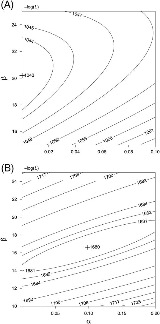
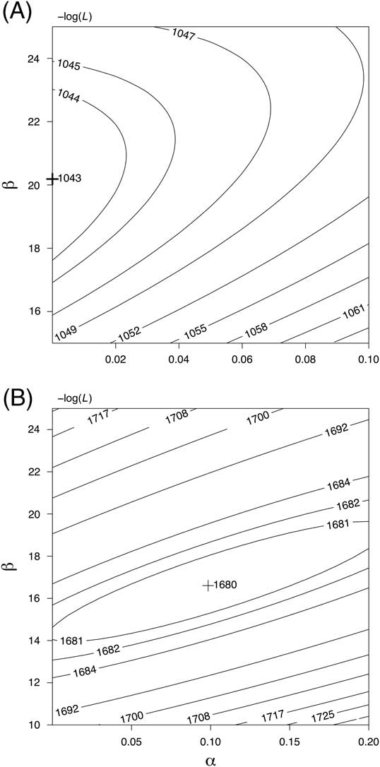
As discussed in the main text, the empirical applications in this paper have used a truncated log-normal distribution for f(p), but I have also explored the beta distribution because of its ability to take on many shapes via combinations of its two parameters, α and β. The beta density f(p) is proportional to p α−1(1−p)β−1, with α>0 and β>0. For most of the stages, the likelihood surface lacks a distinct maximum, steadily increasing toward ever lower values of α. Figure A4A shows a typical example. A less typical case is seen in Figure A4B, in which the likelihood surface has a clear maximum. However, even cases like this are problematic. The maximum-likelihood estimates of α are always much less than 1.0, while estimates of β have an order of magnitude ~10, with the result that the probability distributions have no mode and much of the mass of the distributions lies very close to zero. In the example of Figure A4A, half of the distribution lies below p = 3.3×10⁻⁵, and 87% of it below p=0.01, implying that most genera are so rare that their chances of ever being seen, not to mention having sufficient range and abundance to remain viable, are unrealistically low.
Two examples of likelihood surfaces using the beta distribution to model occupancy probabilities. A, Tremadoc. B, Sandbian. The Tremadoc example is more typical in lacking a distinct peak.