1 Introduction
High-resolution spatial data in the atmosphere and ocean are commonly obtained along one-dimensional horizontal flight, ship or remote-sensing tracks, with instruments measuring the horizontal velocity components and buoyancy, for example. The results of such repeated track measurements are typically reported in terms of estimated power spectra of the relevant physical fields as functions of the one-dimensional along-track wavenumber
 $k$
. A famous example are the atmospheric power spectra from flight tracks during the MOZAIC campaign reported in Nastrom & Gage (Reference Nastrom and Gage1985), and discussed vigorously ever since. Such high-resolution power spectra can offer crucial insights into the nature of the fluid motion at small spatial scales such as the so-called submesoscale range in the ocean, which covers horizontal scales of up to 50 km or so in mid-latitudes (e.g. Callies & Ferrari Reference Callies and Ferrari2013; Callies et al.
Reference Callies, Ferrari, Klymak and Gula2015). At these scales simplistic textbook distinctions between fast gravity waves and slow geostrophic vortical motions (including Rossby waves) break down, and the flow instead exhibits a complex jigsaw puzzle of overlapping and co-mingling wave and vortex motions. Even intermittent bursts of genuine three-dimensional turbulence might conceivably have an impact on the observed small-scale data. Hence, there is a large premium associated with extracting as much information as possible from these costly observations (e.g. Torres et al.
Reference Torres, Klein, Menemenlis, Qiu, Su, Wang, Chen and Fu2018).
In this connection, a linear wave–vortex decomposition method for one-dimensional power spectra has recently been proposed by Bühler, Callies & Ferrari (Reference Bühler, Callies and Ferrari2014) (hereafter BCF14) and then further developed in Callies, Ferrari & Bühler (Reference Callies, Ferrari and Bühler2014), Lindborg (Reference Lindborg2015), Callies, Bühler & Ferrari (Reference Callies, Bühler and Ferrari2016) and Bühler, Kuang & Tabak (Reference Bühler, Kuang and Tabak2017). The BCF14 method is described in § 4.1; in essence, under the assumptions of horizontal isotropy and vertical homogeneity, it performs a decomposition of observed flow spectra into a linear inertia–gravity wave component and a linearly balanced quasi-geostrophic vortex component. Comparing the wave and vortex energy spectra then yields detailed quantitative insights into the relative importance of wave and vortex motions as a function of wavenumber
 $k$
. The method is robust even on noisy data and it is also disarmingly simple to use (see § 4.1), which makes it a convenient tool for data analysis (e.g. Balwada, LaCasce & Speer Reference Balwada, LaCasce and Speer2016; Bierdel et al.
Reference Bierdel, Snyder, Park and Skamarock2016; Rocha et al.
Reference Rocha, Chereskin, Gille and Menemenlis2016a
,Reference Rocha, Gille, Chereskin and Menemenlis
b
; Qiu et al.
Reference Qiu, Nakano, Chen and Klein2017). We note as an aside that the assumptions of horizontal isotropy and vertical homogeneity have been partially relaxed in Callies et al. (Reference Callies, Bühler and Ferrari2016) and Bühler et al. (Reference Bühler, Kuang and Tabak2017), respectively.
The outcome of the BCF14 method in some wavenumber range is most easily interpreted if either the wave energy or the vortex energy completely dominates the spectra in that range. Conversely, if the estimated wave and vortex energies are comparable in magnitude, the physical interpretation is less clear. For example, this is relevant for mesoscale wavenumber range of the upper tropospheric commercial plane flight tracks analysed in Callies et al. (Reference Callies, Bühler and Ferrari2016) (see § 5.1 below). In this situation it is less clear as to how to interpret the results of a linear wave–vortex decomposition, which necessarily omits all nonlinear effects. A number of nonlinear effects are conceivable that could have an impact on the observed spectra, and most of them are hard to investigate based on just the one-dimensional track data at hand.
In the present paper we investigate a specific nonlinear effect, namely the leading-order ageostrophic correction to a balanced quasi-geostrophic vortex flow. This is a classical effect in geophysical fluid dynamics: a time-dependent quasi-geostrophic flow must necessarily be associated with weak vertical velocities that establish the relevant buoyancy structure associated with the balanced flow. The computation of this weak vertical flow is traditionally referred to as solving the omega equation, because omega was the traditional notation for the ‘vertical’ velocity in pressure coordinates (e.g. Holton Reference Holton2004). That equation is a linear elliptic partial differential equation for the vertical velocity with a source term given by certain quadratic combinations of the linear balanced flow fields, which leads to a vertical velocity at next order in the small Rossby number. Now, the key observation here is that a non-zero vertical velocity associated with the balanced vortex flow will robustly project onto the horizontally divergent flow component. In other words, if the true velocity field
 $\boldsymbol{u}=(u,v,w)$
is non-divergent in three dimensions then
 $u_{x}+v_{y}=-w_{z}$
, and hence a non-zero
 $w$
leads to horizontally divergent flow at next order in the Rossby number. This balanced component of the horizontally divergent flow was neglected in the linear BCF14 decomposition and could therefore lead to a false attribution of some of the observed divergent horizontal kinetic energy to the linear wave field, when instead it should be attributed to the balanced vortex field.
We tackle this problem in several steps. First, we investigate quite generally the extent to which the spectra of the ageostrophic correction can be computed from the spectra of the quasi-geostrophic flow. This leads us to a novel power spectral version of the omega equation, which we derive in detail for the shallow-water system and the Boussinesq system. Notably, these equations also hold for anisotropic spectra. Second, we develop a numerical algorithm to compute the ageostrophic correction based on one-dimensional track data, using the assumption of horizontal isotropy. This is a non-trivial question on a number of levels, as will become clear in § 2.2. Significant numerical and mathematical problems have to be overcome to achieve stable and robust results.
We then estimate the size of the ageostrophic correction for actual atmospheric data, but only under the severe limiting assumption that a single vertical scale dominates the balanced flow. This is not very realistic, but by varying this vertical scale we can at least probe the robustness of the BCF14 method for the data sets at hand, i.e. a robust decomposition of the data will change little under this probing. For the atmospheric data we considered, it turns out that the lower stratospheric data are demonstrably robust under this probing, whereas the upper tropospheric data are not, although this latter result depends on the specifics of the data set that is being considered. This sheds some light on the physical nature of the upper tropospheric data, although it falls short of providing a decisive explanation for it.
The structure of the paper is as follows. The omega equation for shallow-water flows is derived and solved for power spectra in §§ 2.1 and 2.2. This is followed by an exploration of the simple link to three-dimensional Boussinesq flows with a single vertical scale in § 2.3. The significant mathematical and numerical task of computing the ageostrophic spectra from one-dimensional track data is tackled in § 3 and its role in wave–vortex decompositions is worked out and tested in § 4. The method is finally applied to atmospheric data sets in § 5 and some concluding comments are offered in 6.
2 Statistical omega equations for power spectra
We first derive a standard omega equation for a shallow-water system, which allows computation at leading order in Rossby number of the ageostrophic velocity potential from a single realization of a quasi-geostrophic stream function. This is followed by a detailed investigation of how to compute the ageostrophic energy spectrum from the quasi-geostrophic stream function spectrum, which can be done under the assumption of independent Fourier components. This involves a new, power spectral version of the omega equation. Finally, we consider how the shallow-water theory can be applied to a three-dimensional Boussinesq model under the assumption of a single dominant vertical wavenumber.
2.1 The omega equation for shallow water
This derivation uses standard methods, but we provide full details because we have not found a reference for it in the literature. We consider the standard shallow-water system without topography on an
 $f$
-plane:
 $$\begin{eqnarray}\frac{\text{D}\boldsymbol{u}}{\text{D}t}+\boldsymbol{f}\times \boldsymbol{u}+g\unicode[STIX]{x1D735}\unicode[STIX]{x1D702}=0,\quad \frac{\text{D}\unicode[STIX]{x1D702}}{\text{D}t}+(\unicode[STIX]{x1D702}+H)\unicode[STIX]{x1D735}\boldsymbol{\cdot }\boldsymbol{u}=0.\end{eqnarray}$$
Here
 $\text{D}/\text{D}t=\unicode[STIX]{x2202}/\unicode[STIX]{x2202}t+\boldsymbol{u}\boldsymbol{\cdot }\unicode[STIX]{x1D735}$
is the material derivative,
 $\boldsymbol{u}=(u,v)$
is the horizontal velocity vector,
 $\boldsymbol{f}=f\boldsymbol{e}_{\boldsymbol{z}}$
is the constant Coriolis vector,
 $g$
is gravity,
 $\unicode[STIX]{x1D702}$
is the layer depth fluctuation and
 $H$
is the rest layer depth. Using the standard Helmholtz decomposition (subscripts denote derivatives)
 $$\begin{eqnarray}\displaystyle u=\unicode[STIX]{x1D719}_{x}-\unicode[STIX]{x1D713}_{y}\quad \text{and}\quad v=\unicode[STIX]{x1D719}_{y}+\unicode[STIX]{x1D713}_{x} & & \displaystyle\end{eqnarray}$$
in terms of a velocity potential
 $\unicode[STIX]{x1D719}$
and stream function
 $\unicode[STIX]{x1D713}$
, the shallow-water vorticity equation is
 $$\begin{eqnarray}\displaystyle & \displaystyle \frac{\unicode[STIX]{x2202}}{\unicode[STIX]{x2202}t}\unicode[STIX]{x1D6FB}^{2}\unicode[STIX]{x1D713}+J\left(\unicode[STIX]{x1D713},\unicode[STIX]{x1D6FB}^{2}\unicode[STIX]{x1D713}\right)+(\unicode[STIX]{x1D735}\unicode[STIX]{x1D719}\boldsymbol{\cdot }\unicode[STIX]{x1D735})\unicode[STIX]{x1D6FB}^{2}\unicode[STIX]{x1D713}+\left(f+\unicode[STIX]{x1D6FB}^{2}\unicode[STIX]{x1D713}\right)\unicode[STIX]{x1D6FB}^{2}\unicode[STIX]{x1D719}=0. & \displaystyle\end{eqnarray}$$
Here
 $J\left(A,B\right)=A_{x}B_{y}-A_{y}B_{x}$
is the Jacobian operator. We now apply the subscript ‘
 $V$
’ to indicate that we are considering a low-Rossby-number vortical flow. This flow is described at first and second order in Rossby number by a quasi-geostrophic stream function
 $\unicode[STIX]{x1D713}_{V}$
and by an ageostrophic velocity potential
 $\unicode[STIX]{x1D719}_{V}$
, respectively. The leading-order approximation of the vorticity budget (2.3) is then
 $$\begin{eqnarray}\displaystyle \frac{\unicode[STIX]{x2202}}{\unicode[STIX]{x2202}t} & \displaystyle \unicode[STIX]{x1D6FB}^{2}\unicode[STIX]{x1D713}_{V}+J(\unicode[STIX]{x1D713}_{V},\unicode[STIX]{x1D6FB}^{2}\unicode[STIX]{x1D713}_{V})+f\unicode[STIX]{x1D6FB}^{2}\unicode[STIX]{x1D719}_{V}=0. & \displaystyle\end{eqnarray}$$
The stream function
 $\unicode[STIX]{x1D713}_{V}$
obeys the usual quasi-geostrophic equations
 $$\begin{eqnarray}\displaystyle & \displaystyle (\unicode[STIX]{x1D6FB}^{2}-\unicode[STIX]{x1D705}_{D}^{2})\frac{\unicode[STIX]{x2202}\unicode[STIX]{x1D713}_{V}}{\unicode[STIX]{x2202}t}+J(\unicode[STIX]{x1D713}_{V},\unicode[STIX]{x1D6FB}^{2}\unicode[STIX]{x1D713}_{V})=0,\quad \text{where }\unicode[STIX]{x1D705}_{D}=\frac{f}{\sqrt{gH}} & \displaystyle\end{eqnarray}$$
is the deformation wavenumber. Applying
 $\unicode[STIX]{x1D6FB}^{2}-\unicode[STIX]{x1D705}_{D}^{2}$
to (2.4),
 $\unicode[STIX]{x1D6FB}^{2}$
to (2.5) and subtracting then leads to the shallow-water omega equation
 $$\begin{eqnarray}\displaystyle & \displaystyle \left(\unicode[STIX]{x1D6FB}^{2}-\unicode[STIX]{x1D705}_{D}^{2}\right)\unicode[STIX]{x1D6FB}^{2}\unicode[STIX]{x1D719}_{V}=\frac{\unicode[STIX]{x1D705}_{D}^{2}}{f}J\left(\unicode[STIX]{x1D713}_{V},\unicode[STIX]{x1D6FB}^{2}\unicode[STIX]{x1D713}_{V}\right). & \displaystyle\end{eqnarray}$$
With suitable boundary conditions, this elliptic partial differential equation allows computing
 $\unicode[STIX]{x1D719}_{V}$
from
 $\unicode[STIX]{x1D713}_{V}$
.
2.2 The omega relation between the power spectra of
 $\unicode[STIX]{x1D719}_{V}$
and
$\unicode[STIX]{x1D713}_{V}$


The simplest relevant setting involves a zero-mean random stream function
 $\unicode[STIX]{x1D713}_{V}$
with homogeneous statistics in a doubly periodic square domain with length
 $L$
. As is well known (e.g. Yaglom Reference Yaglom1952), such a random function is naturally represented by a Fourier series (we omit the time variable
 $t$
here)
 $$\begin{eqnarray}\displaystyle & \displaystyle \unicode[STIX]{x1D713}_{V}(x,y)=\frac{1}{L^{2}}\mathop{\sum }_{k,l}\widehat{\unicode[STIX]{x1D713}}_{V}(k,l)\,\text{e}^{\text{i}(kx+ly)},\quad k,l\in \left\{0,\pm \frac{2\unicode[STIX]{x03C0}}{L},\ldots \right\}, & \displaystyle\end{eqnarray}$$
where the collection of Fourier coefficients
 $\widehat{\unicode[STIX]{x1D713}}_{V}(k,l)$
are uncorrelated zero-mean random variables. Specifically, we have the reality condition
 $$\begin{eqnarray}\displaystyle \widehat{\unicode[STIX]{x1D713}}_{V}(k,l)=\widehat{\unicode[STIX]{x1D713}}_{V}^{\ast }(-k,-l), & & \displaystyle\end{eqnarray}$$
and the statistical conditions
 $$\begin{eqnarray}\displaystyle \overline{\widehat{\unicode[STIX]{x1D713}}_{V}(k,l)}=0\quad \text{and}\quad \overline{\widehat{\unicode[STIX]{x1D713}}_{V}^{\ast }(k_{1},l_{1})\widehat{\unicode[STIX]{x1D713}}_{V}(k_{2},l_{2})}=L^{2}\unicode[STIX]{x1D6FF}_{k_{1}k_{2}}\unicode[STIX]{x1D6FF}_{l_{1}l_{2}}\,S_{V}^{\unicode[STIX]{x1D713}}(k_{1},l_{1}), & & \displaystyle\end{eqnarray}$$
where the overbar denotes taking the statistical expectation. The real-valued non-negative
 $S_{V}^{\unicode[STIX]{x1D713}}=\overline{|\widehat{\unicode[STIX]{x1D713}}_{V}|^{2}}/L^{2}$
is the power spectrum of
 $\unicode[STIX]{x1D713}_{V}$
. By the Wiener–Khinchin theorem (e.g. Yaglom Reference Yaglom1952; Champeney Reference Champeney1987), the power spectrum is the Fourier transform of the covariance function, so we also have
 $$\begin{eqnarray}\displaystyle C_{V}^{\unicode[STIX]{x1D713}}(x,y)\equiv \overline{\unicode[STIX]{x1D713}(x_{0},y_{0})\unicode[STIX]{x1D713}(x_{0}+x,y_{0}+y)}=\frac{1}{L^{2}}\mathop{\sum }_{k,l}S_{V}^{\unicode[STIX]{x1D713}}(k,l)\,\text{e}^{\text{i}(kx+ly)}. & & \displaystyle\end{eqnarray}$$
By homogeneity, the variables
 $(x_{0},y_{0})$
are arbitrary in the definition of the covariance function
 $C_{V}^{\unicode[STIX]{x1D713}}$
.
We now explore the consequences of (2.6) for the relation between the power spectra of
 $\unicode[STIX]{x1D719}_{V}$
and
 $\unicode[STIX]{x1D713}_{V}$
. Of course, if we had complete statistical information about
 $\unicode[STIX]{x1D713}_{V}$
then we could in principle generate an ensemble of random samples of
 $\unicode[STIX]{x1D713}_{V}$
, calculate the corresponding samples of
 $\unicode[STIX]{x1D719}_{V}$
directly from (2.6) and finally compute its power spectrum directly. However, such complete statistical information is typically absent in practice, where observational results are often limited to power spectra. But many different random functions can have the same power spectra, which makes the general problem of computing
 $S_{V}^{\unicode[STIX]{x1D719}}$
from
 $S_{V}^{\unicode[STIX]{x1D713}}$
non-unique. This can also affect the cross-correlation between
 $\unicode[STIX]{x1D719}_{V}$
and
 $\unicode[STIX]{x1D713}_{V}$
. (An example is given in appendix A.)
A natural way to turn this into a well-posed problem is to make the assumption that the Fourier components
 $\widehat{\unicode[STIX]{x1D713}}_{V}(k,l)$
are not just uncorrelated, as dictated by homogeneity, but are in fact mutually independent for different
 $(k,l)$
(except when the reality condition (2.8) enforces otherwise). The validity of this assumption is by no means self-evident on physical grounds. Nevertheless, it encompasses several standard methods for the physical modelling of homogeneous random functions, such as Gaussian random fields (where the Fourier coefficients are independent Gaussian random variables), or the random-phase approximation (where the magnitude of the complex Fourier coefficients is fixed, but their phases are independent uniform random variables). Under this assumption we can now derive closed-form exact formulas for
 $\unicode[STIX]{x1D719}_{V}$
and
 $S_{V}^{\unicode[STIX]{x1D719}}$
and also show that
 $\unicode[STIX]{x1D713}_{V}$
and
 $\unicode[STIX]{x1D719}_{V}$
are uncorrelated.
The source term in (2.6) can be written as
 $$\begin{eqnarray}\displaystyle & \displaystyle J(\unicode[STIX]{x1D713}_{V},\unicode[STIX]{x1D6FB}^{2}\unicode[STIX]{x1D713}_{V})=\frac{1}{2L^{4}}\,\mathop{\sum }_{\boldsymbol{k}_{1},\boldsymbol{k}_{2}}\,\hat{\unicode[STIX]{x1D713}}_{1}\hat{\unicode[STIX]{x1D713}}_{2}\,(\unicode[STIX]{x1D705}_{2}^{2}-\unicode[STIX]{x1D705}_{1}^{2})(\boldsymbol{k}_{1}\times \boldsymbol{k}_{2})\text{e}^{\text{i}(\boldsymbol{k}_{1}+\boldsymbol{k}_{2})\boldsymbol{\cdot }\boldsymbol{x}}. & \displaystyle\end{eqnarray}$$
Here
 $\boldsymbol{k}=(k,l)$
is the horizontal wavenumber vector with magnitude
 $\unicode[STIX]{x1D705}=|\boldsymbol{k}|$
,
 $\hat{\unicode[STIX]{x1D713}}_{1}$
and
 $\hat{\unicode[STIX]{x1D713}}_{2}$
are shorthand for
 $\hat{\unicode[STIX]{x1D713}}_{V}(\boldsymbol{k}_{1})$
and
 $\hat{\unicode[STIX]{x1D713}}_{V}(\boldsymbol{k}_{2})$
, the two-dimensional cross-product
 $(\boldsymbol{k}_{1}\times \boldsymbol{k}_{2})=k_{1}l_{2}-k_{2}l_{1}$
and
 $\boldsymbol{x}=(x,y)$
. This formula is derived by direct substitution followed by symmetrization over the dummy indices
 $1$
and
 $2$
(e.g. p. 234 of Salmon Reference Salmon1998). It makes explicit that the Jacobian is non-zero only for non-parallel pairs of wavenumber vectors with unequal magnitude
 $\unicode[STIX]{x1D705}_{1}\neq \unicode[STIX]{x1D705}_{2}$
. The Fourier transform of (2.6) yields
 $$\begin{eqnarray}\displaystyle & \displaystyle \hat{\unicode[STIX]{x1D719}}_{V}(\boldsymbol{k})=\frac{\unicode[STIX]{x1D705}_{D}^{2}/f}{\unicode[STIX]{x1D705}^{2}(\unicode[STIX]{x1D705}^{2}+\unicode[STIX]{x1D705}_{D}^{2})}\frac{1}{2L^{2}}\,\mathop{\sum }_{\boldsymbol{k}=\boldsymbol{k}_{1}+\boldsymbol{k}_{2}}\,\hat{\unicode[STIX]{x1D713}}_{1}\hat{\unicode[STIX]{x1D713}}_{2}\,(\unicode[STIX]{x1D705}_{2}^{2}-\unicode[STIX]{x1D705}_{1}^{2})(\boldsymbol{k}_{1}\times \boldsymbol{k}_{2}). & \displaystyle\end{eqnarray}$$
Now, the cross-spectrum between
 $\unicode[STIX]{x1D713}_{V}$
and
 $\unicode[STIX]{x1D719}_{V}$
is
 $$\begin{eqnarray}\displaystyle & \displaystyle \overline{\hat{\unicode[STIX]{x1D713}}_{V}^{\ast }\hat{\unicode[STIX]{x1D719}}_{V}}/L^{2}=\frac{\unicode[STIX]{x1D705}_{D}^{2}/f}{\unicode[STIX]{x1D705}^{2}(\unicode[STIX]{x1D705}^{2}+\unicode[STIX]{x1D705}_{D}^{2})}\frac{1}{2L^{2}}\,\mathop{\sum }_{\boldsymbol{k}=\boldsymbol{k}_{1}+\boldsymbol{k}_{2}}\,\overline{\hat{\unicode[STIX]{x1D713}}_{V}(\boldsymbol{k})\hat{\unicode[STIX]{x1D713}}_{1}\hat{\unicode[STIX]{x1D713}}_{2}}\,(\unicode[STIX]{x1D705}_{2}^{2}-\unicode[STIX]{x1D705}_{1}^{2})(\boldsymbol{k}_{1}\times \boldsymbol{k}_{2}). & \displaystyle\end{eqnarray}$$
This requires knowledge of triple correlations, so knowledge of the quadratic power spectra is insufficient. However, under the assumption of independent Fourier coefficients the triple correlation
 $\overline{\hat{\unicode[STIX]{x1D713}}_{V}(\boldsymbol{k})\hat{\unicode[STIX]{x1D713}}_{1}\hat{\unicode[STIX]{x1D713}}_{2}}$
can be non-zero only for terms with
 $\boldsymbol{k}=\pm \boldsymbol{k}_{1}$
or
 $\boldsymbol{k}=\pm \boldsymbol{k}_{2}$
. But then
 $\boldsymbol{k}=\boldsymbol{k}_{1}+\boldsymbol{k}_{2}$
implies that
 $(\boldsymbol{k}_{1},\boldsymbol{k}_{2})$
are parallel and therefore the cross-product is zero. Hence all terms in the sum vanish, the cross-spectrum is zero and
 $\unicode[STIX]{x1D713}_{V}$
and
 $\unicode[STIX]{x1D719}_{V}$
are indeed uncorrelated.
Similar reasoning can be applied to
 $$\begin{eqnarray}\overline{|\hat{\unicode[STIX]{x1D719}}_{V}|^{2}}=\left(\frac{\unicode[STIX]{x1D705}_{D}^{2}/f}{\unicode[STIX]{x1D705}^{2}(\unicode[STIX]{x1D705}^{2}+\unicode[STIX]{x1D705}_{D}^{2})}\right)^{2}\frac{1}{4L^{4}}\,\mathop{\sum }_{\substack{ \boldsymbol{k}=\boldsymbol{k}_{1}+\boldsymbol{k}_{2} \\ \boldsymbol{k}=\boldsymbol{k}_{3}+\boldsymbol{k}_{4}}}\,\overline{\hat{\unicode[STIX]{x1D713}}_{1}\hat{\unicode[STIX]{x1D713}}_{2}\hat{\unicode[STIX]{x1D713}}_{3}^{\ast }\hat{\unicode[STIX]{x1D713}}_{4}^{\ast }}\,(\unicode[STIX]{x1D705}_{2}^{2}-\unicode[STIX]{x1D705}_{1}^{2})(\boldsymbol{k}_{1}\times \boldsymbol{k}_{2})(\unicode[STIX]{x1D705}_{4}^{2}-\unicode[STIX]{x1D705}_{3}^{2})(\boldsymbol{k}_{3}\times \boldsymbol{k}_{4}).\end{eqnarray}$$
This quadruple sum over
 $(\boldsymbol{k}_{1},\boldsymbol{k}_{2},\boldsymbol{k}_{3},\boldsymbol{k}_{4})$
under the constraints
 $\boldsymbol{k}=\boldsymbol{k}_{1}+\boldsymbol{k}_{2}=\boldsymbol{k}_{3}+\boldsymbol{k}_{4}$
again greatly simplifies for independent Fourier components. First, terms for which
 $\boldsymbol{k}_{1}=\pm \boldsymbol{k}_{2}$
or
 $\boldsymbol{k}_{3}=\pm \boldsymbol{k}_{4}$
again vanish because of collinearity. This leaves only the two cases
 $(\boldsymbol{k}_{1}=\boldsymbol{k}_{3},\boldsymbol{k}_{2}=\boldsymbol{k}_{4})$
and
 $(\boldsymbol{k}_{1}=\boldsymbol{k}_{4},\boldsymbol{k}_{2}=\boldsymbol{k}_{3})$
to consider. Because
 $\boldsymbol{k}_{1}\neq \boldsymbol{k}_{2}$
(to avoid collinearity), the quadruple correlation
 $\overline{\hat{\unicode[STIX]{x1D713}}_{1}\hat{\unicode[STIX]{x1D713}}_{2}\hat{\unicode[STIX]{x1D713}}_{3}^{\ast }\hat{\unicode[STIX]{x1D713}}_{4}^{\ast }}=\overline{|\hat{\unicode[STIX]{x1D713}}_{1}|^{2}}\;\overline{|\hat{\unicode[STIX]{x1D713}}_{2}|^{2}}$
in both cases. Therefore it is enough to consider just the first case and then multiply the result by two. The end result is the explicit double sum linking the power spectra
 $S_{V}^{\unicode[STIX]{x1D713}}$
and
 $S_{V}^{\unicode[STIX]{x1D719}}=\overline{|\hat{\unicode[STIX]{x1D719}}_{V}|^{2}}/L^{2}$
:
 $$\begin{eqnarray}S_{V}^{\unicode[STIX]{x1D719}}(\boldsymbol{k})=\left(\frac{\unicode[STIX]{x1D705}_{D}^{2}/f}{\unicode[STIX]{x1D705}^{2}(\unicode[STIX]{x1D705}^{2}+\unicode[STIX]{x1D705}_{D}^{2})}\right)^{2}\frac{1}{2L^{2}}\,\mathop{\sum }_{\boldsymbol{k}=\boldsymbol{k}_{1}+\boldsymbol{k}_{2}}\,S_{V}^{\unicode[STIX]{x1D713}}(\boldsymbol{k}_{1})S_{V}^{\unicode[STIX]{x1D713}}(\boldsymbol{k}_{2})\,|(\unicode[STIX]{x1D705}_{2}^{2}-\unicode[STIX]{x1D705}_{1}^{2})(\boldsymbol{k}_{1}\times \boldsymbol{k}_{2})|^{2}.\end{eqnarray}$$
To our knowledge, this statistical omega equation for power spectra is new. We note that the right-hand side can be evaluated quickly using a pseudospectral method (see appendix B).
It is instructive to rewrite (2.15) in terms of energy spectra. For example, using the divergent and rotational kinetic energy spectra
 $$\begin{eqnarray}\displaystyle K_{\unicode[STIX]{x1D719},V}=\frac{\unicode[STIX]{x1D705}^{2}}{2}S_{V}^{\unicode[STIX]{x1D719}}\quad \text{and}\quad K_{\unicode[STIX]{x1D713},V}=\frac{\unicode[STIX]{x1D705}^{2}}{2}S_{V}^{\unicode[STIX]{x1D713}}, & & \displaystyle\end{eqnarray}$$
equation (2.15) takes the alternative form
 $$\begin{eqnarray}K_{\unicode[STIX]{x1D719},V}(\boldsymbol{k})=\left(\frac{\unicode[STIX]{x1D705}_{D}^{2}/f}{\unicode[STIX]{x1D705}(\unicode[STIX]{x1D705}^{2}+\unicode[STIX]{x1D705}_{D}^{2})}\right)^{2}\frac{1}{L^{2}}\,\mathop{\sum }_{\boldsymbol{k}=\boldsymbol{k}_{1}+\boldsymbol{k}_{2}}\,\frac{K_{\unicode[STIX]{x1D713},V}(\boldsymbol{k}_{1})K_{\unicode[STIX]{x1D713},V}(\boldsymbol{k}_{2})}{\unicode[STIX]{x1D705}_{1}^{2}\unicode[STIX]{x1D705}_{2}^{2}}\,|(\unicode[STIX]{x1D705}_{2}^{2}-\unicode[STIX]{x1D705}_{1}^{2})(\boldsymbol{k}_{1}\times \boldsymbol{k}_{2})|^{2}.\end{eqnarray}$$
Common to both forms is the observation that, all other things being equal, the ageostrophic response is an increasing function of the deformation wavenumber
 $\unicode[STIX]{x1D705}_{D}$
. However, this is not necessarily true if we rewrite the relation in terms of the energy spectra, which include available potential energy in the geostrophic stream function part. Specifically,
 $$\begin{eqnarray}\displaystyle & \displaystyle E_{\unicode[STIX]{x1D719},V}=K_{\unicode[STIX]{x1D719},V}\quad \text{and}\quad E_{\unicode[STIX]{x1D713},V}=K_{\unicode[STIX]{x1D713},V}+\frac{\unicode[STIX]{x1D705}_{D}^{2}}{2}S_{V}^{\unicode[STIX]{x1D713}} & \displaystyle\end{eqnarray}$$
imply that
 $$\begin{eqnarray}E_{\unicode[STIX]{x1D719},V}(\boldsymbol{k})=\left(\frac{\unicode[STIX]{x1D705}_{D}^{2}/f}{\unicode[STIX]{x1D705}(\unicode[STIX]{x1D705}^{2}+\unicode[STIX]{x1D705}_{D}^{2})}\right)^{2}\frac{1}{L^{2}}\,\mathop{\sum }_{\boldsymbol{k}=\boldsymbol{k}_{1}+\boldsymbol{k}_{2}}\,\frac{E_{\unicode[STIX]{x1D713},V}(\boldsymbol{k}_{1})E_{\unicode[STIX]{x1D713},V}(\boldsymbol{k}_{2})}{(\unicode[STIX]{x1D705}_{1}^{2}+\unicode[STIX]{x1D705}_{D}^{2})(\unicode[STIX]{x1D705}_{2}^{2}+\unicode[STIX]{x1D705}_{D}^{2})}\,|(\unicode[STIX]{x1D705}_{2}^{2}-\unicode[STIX]{x1D705}_{1}^{2})(\boldsymbol{k}_{1}\times \boldsymbol{k}_{2})|^{2}.\end{eqnarray}$$
Now the dependence on
 $\unicode[STIX]{x1D705}_{D}$
is not monotonic. For example, consider quasi-geostrophic energy spectra
 $E_{\unicode[STIX]{x1D713},V}$
whose support is restricted to wavenumbers that are much smaller than
 $\unicode[STIX]{x1D705}_{D}$
. For such spectra (2.19) is well approximated by
 $$\begin{eqnarray}\displaystyle & \displaystyle E_{\unicode[STIX]{x1D719},V}(\boldsymbol{k})\approx \left(\frac{1/f}{\unicode[STIX]{x1D705}\unicode[STIX]{x1D705}_{D}^{2}}\right)^{2}\frac{1}{L^{2}}\,\mathop{\sum }_{\boldsymbol{k}=\boldsymbol{k}_{1}+\boldsymbol{k}_{2}}\,E_{\unicode[STIX]{x1D713},V}(\boldsymbol{k}_{1})E_{\unicode[STIX]{x1D713},V}(\boldsymbol{k}_{2})\,|(\unicode[STIX]{x1D705}_{2}^{2}-\unicode[STIX]{x1D705}_{1}^{2})(\boldsymbol{k}_{1}\times \boldsymbol{k}_{2})|^{2}, & \displaystyle\end{eqnarray}$$
which clearly decreases with
 $\unicode[STIX]{x1D705}_{D}$
. Physically, this corresponds to quasi-geostrophic motion on scales much larger than the deformation radius, e.g. planetary geostrophic motion.
2.3 Boussinesq model with single vertical mode
The omega equation for the hydrostatic Boussinesq system with constant buoyancy frequency
 $N$
and Coriolis frequency
 $f$
is well known. For example, following Davies (Reference Davies2015), in its ‘conventional’ form it relates
 $\unicode[STIX]{x1D713}_{V}(x,y,z)$
and
 $\unicode[STIX]{x1D719}_{V}(x,y,z)$
via
 $$\begin{eqnarray}-\left(\unicode[STIX]{x1D6FB}^{2}+\frac{f^{2}}{N^{2}}\frac{\unicode[STIX]{x2202}^{2}}{\unicode[STIX]{x2202}z^{2}}\right)\unicode[STIX]{x1D6FB}^{2}\unicode[STIX]{x1D719}_{V}=-\frac{f}{N^{2}}\unicode[STIX]{x1D6FB}^{2}J\left(\unicode[STIX]{x1D713}_{V},\frac{\unicode[STIX]{x2202}^{2}\unicode[STIX]{x1D713}_{V}}{\unicode[STIX]{x2202}z^{2}}\right)+\frac{f}{N^{2}}\frac{\unicode[STIX]{x2202}^{2}}{\unicode[STIX]{x2202}z^{2}}(J(\unicode[STIX]{x1D713}_{V},\unicode[STIX]{x1D6FB}^{2}\unicode[STIX]{x1D713}_{V})).\end{eqnarray}$$
Here
 $\unicode[STIX]{x1D6FB}^{2}$
and
 $J(\cdot ,\cdot )$
operate in the horizontal only, as before. The vertical velocity
 $w$
then follows from
 $w_{z}=-(u_{x}+v_{y})=-\unicode[STIX]{x1D6FB}^{2}\unicode[STIX]{x1D719}_{V}$
. This equation can straightforwardly be solved for
 $\unicode[STIX]{x1D719}_{V}$
if
 $\unicode[STIX]{x1D713}_{V}$
is known. The corresponding power spectral omega equation is given in appendix C.
However, (2.21) is too general to be of use in the statistical analysis of horizontal track data obtained at a fixed altitude
 $z$
. This is because the statistics of the vertical derivatives that enter (2.21) are unknown (see appendix C for details). On the other hand, (2.21) yields a statistical equation purely in the horizontal coordinates if we assume that the flow in the area of interest is dominated by a single vertical mode with wavenumber
 $m_{\ast }$
, say. For given track data, this equation then allows us to study the potential relevance of the ageostrophic
 $\unicode[STIX]{x1D719}_{V}$
by varying that wavenumber
 $m_{\ast }$
. We will now derive this equation, which will turn out to be a variant of the shallow-water omega equation (2.6). We assume that
 $$\begin{eqnarray}\displaystyle \unicode[STIX]{x1D713}_{V}(x,y,z)=\widetilde{\unicode[STIX]{x1D713}}_{V}(x,y)[a\cos (m_{\ast }z)+b\sin (m_{\ast }z)], & & \displaystyle\end{eqnarray}$$
where
 $a$
and
 $b$
are independent Gaussian zero-mean random variables with unit variance,
 $m_{\ast }$
is a fixed wavenumber and
 $\widetilde{\unicode[STIX]{x1D713}}_{V}(x,y)$
is a zero-mean random function (independent of
 $a$
and
 $b$
) with horizontally homogeneous statistics. It follows that
 $$\begin{eqnarray}\displaystyle \overline{\unicode[STIX]{x1D713}_{V}(x_{1},y_{1},z_{1})\unicode[STIX]{x1D713}_{V}(x_{2},y_{2},z_{2})}=\overline{\widetilde{\unicode[STIX]{x1D713}}_{V}(x_{1},y_{1})\widetilde{\unicode[STIX]{x1D713}}_{V}(x_{2},y_{2})}\cos (m_{\ast }(z_{1}-z_{2})). & & \displaystyle\end{eqnarray}$$
For fixed-altitude track data only
 $z_{1}=z_{2}$
is relevant, so this reduces to a horizontal covariance. Denoting
 $C_{V}^{\unicode[STIX]{x1D713}}(x,y,0)$
by
 $C_{V}^{\unicode[STIX]{x1D713}}(x,y)$
we find
 $$\begin{eqnarray}\displaystyle C_{V}^{\unicode[STIX]{x1D713}}(x,y)=\overline{\widetilde{\unicode[STIX]{x1D713}}_{V}(0,0)\widetilde{\unicode[STIX]{x1D713}}_{V}(x,y)}. & & \displaystyle\end{eqnarray}$$
Now, with (2.22) the vertical derivatives in (2.21) can be evaluated explicitly. In particular, the term
 $J(\unicode[STIX]{x1D713}_{V},\unicode[STIX]{x2202}^{2}\unicode[STIX]{x1D713}_{V}/\unicode[STIX]{x2202}z^{2})$
vanishes, and a short calculation shows that
 $\unicode[STIX]{x1D719}_{V}(x,y,z)$
can be written as
 $$\begin{eqnarray}\displaystyle & \displaystyle \unicode[STIX]{x1D719}_{V}(x,y,z)=\widetilde{\unicode[STIX]{x1D719}}_{V}(x,y)\left[\frac{a^{2}-b^{2}}{2}\cos (2m_{\ast }z)+ab\sin (2m_{\ast }z)\right]. & \displaystyle\end{eqnarray}$$
Here
 $\widetilde{\unicode[STIX]{x1D719}}_{V}(x,y)$
satisfies
 $$\begin{eqnarray}\displaystyle & \displaystyle \left(\unicode[STIX]{x1D6FB}^{2}-\frac{f^{2}}{N^{2}}4m_{\ast }^{2}\right)\unicode[STIX]{x1D6FB}^{2}\widetilde{\unicode[STIX]{x1D719}}_{V}(x,y)=\frac{f}{N^{2}}4m_{\ast }^{2}J(\widetilde{\unicode[STIX]{x1D713}}_{V}(x,y),\unicode[STIX]{x1D6FB}^{2}\widetilde{\unicode[STIX]{x1D713}}_{V}(x,y)), & \displaystyle\end{eqnarray}$$
which is the shallow-water omega equation (2.6) with
 $\unicode[STIX]{x1D705}_{D}$
replaced by
 $$\begin{eqnarray}\displaystyle & \displaystyle \unicode[STIX]{x1D705}_{\ast }=2m_{\ast }\frac{f}{N}. & \displaystyle\end{eqnarray}$$
The horizontal covariance at a fixed level
 $z=0$
, say, is then
 $$\begin{eqnarray}\displaystyle C_{V}^{\unicode[STIX]{x1D719}}(x,y)=\overline{\widetilde{\unicode[STIX]{x1D719}}_{V}(0,0)\widetilde{\unicode[STIX]{x1D719}}_{V}(x,y)}\overline{\left(\frac{a^{2}-b^{2}}{2}\right)^{2}}=\overline{\widetilde{\unicode[STIX]{x1D719}}_{V}(0,0)\widetilde{\unicode[STIX]{x1D719}}_{V}(x,y)}. & & \displaystyle\end{eqnarray}$$
This uses the Gaussian property
 $\overline{a^{4}}=3\overline{a^{2}}$
. Hence, the shallow-water power spectral omega equation extends naturally to the Boussinesq system with a single vertical mode.
3 Application to one-dimensional spectra with horizontal isotropy
So far we have derived statistical versions of the omega equation, but these equations still contain multi-dimensional spectral data. We now proceed with the difficult step of descending to omega relations that link one-dimensional spectra such as those obtained along measurement tracks. Specifically, we seek to compute numerically the ageostrophic correction
 $S_{V}^{\unicode[STIX]{x1D719}}$
defined in (2.15) purely from one-dimensional horizontal track data under the assumption of horizontal isotropy. For definiteness, we align the
 $x$
-axis with the track so we are collecting data at
 $y=0$
. This yields
 $C_{V}^{\unicode[STIX]{x1D713}}(x,0)$
, or the equivalent one-dimensional spectrum
 $$\begin{eqnarray}\displaystyle & \displaystyle S_{V}^{\unicode[STIX]{x1D713}}(k)=\frac{1}{2\unicode[STIX]{x03C0}}\int S_{V}^{\unicode[STIX]{x1D713}}(k,l)\,\text{d}l. & \displaystyle\end{eqnarray}$$
(Here and in the following we work with continuous spectra for computational simplicity, but the corresponding formulas for discrete spectra follow easily by replacing spectral integrals with sums and
 $\text{d}l$
by
 $2\unicode[STIX]{x03C0}/L$
.) Basically, our task is to compute a nonlinear map
 $$\begin{eqnarray}\displaystyle S_{V}^{\unicode[STIX]{x1D713}}(k)\longmapsto S_{V}^{\unicode[STIX]{x1D719}}(k) & & \displaystyle\end{eqnarray}$$
between the one-dimensional spectra that is consistent with (2.15) under the assumption that the underlying flow statistics are isotropic in the horizontal plane. This means that
 $C_{V}^{\unicode[STIX]{x1D713}}(x,y)$
is a function of
 $r=\sqrt{x^{2}+y^{2}}$
only, so
 $$\begin{eqnarray}\displaystyle & \displaystyle C_{V}^{\unicode[STIX]{x1D713}}(x,y)=g(r)\quad \text{and}\quad S_{V}^{\unicode[STIX]{x1D713}}(k,l)={\mathcal{F}}_{2}[g(r)]={\hat{g}}(\unicode[STIX]{x1D705}), & \displaystyle\end{eqnarray}$$
where
 $\unicode[STIX]{x1D705}=\sqrt{k^{2}+l^{2}}$
and
 $$\begin{eqnarray}\displaystyle {\mathcal{F}}_{2}[f(x,y)]=\iint f(x,y)\text{e}^{-\text{i}(kx+ly)}\,\text{d}x\,\text{d}y & & \displaystyle\end{eqnarray}$$
is the two-dimensional Fourier transform. Isotropic stream function spectra imply isotropic potential spectra, so we also have
 $$\begin{eqnarray}\displaystyle S_{V}^{\unicode[STIX]{x1D719}}(k,l)={\hat{h}}(\unicode[STIX]{x1D705}), & & \displaystyle\end{eqnarray}$$
for a function
 ${\hat{h}}(\unicode[STIX]{x1D705})$
to be found. The observable one-dimensional spectrum
 $S_{V}^{\unicode[STIX]{x1D719}}(k)$
is then the Abel transform of
 ${\hat{h}}(\unicode[STIX]{x1D705})$
divided by
 $2\unicode[STIX]{x03C0}$
, i.e.
 $$\begin{eqnarray}\displaystyle & \displaystyle S_{V}^{\unicode[STIX]{x1D719}}(k)=\frac{1}{2\unicode[STIX]{x03C0}}\int _{-\infty }^{\infty }{\hat{h}}(\unicode[STIX]{x1D705})\,\text{d}l=\frac{1}{\unicode[STIX]{x03C0}}\int _{k}^{\infty }\frac{{\hat{h}}(\unicode[STIX]{x1D705})\unicode[STIX]{x1D705}}{\sqrt{\unicode[STIX]{x1D705}^{2}-k^{2}}}\,\text{d}\unicode[STIX]{x1D705},\quad k\geqslant 0. & \displaystyle\end{eqnarray}$$
The same is true for
 $S_{V}^{\unicode[STIX]{x1D713}}(k)$
, which is the Abel transform of
 ${\hat{g}}(\unicode[STIX]{x1D705})$
. The task is now to compute the desired
 $S_{V}^{\unicode[STIX]{x1D719}}(k)$
from the observed
 $S_{V}^{\unicode[STIX]{x1D713}}(k)$
.
3.1 First method using Abel inverse transform
A natural first method is as follows: apply an Abel inverse transform to the one-dimensional
 $S_{V}^{\unicode[STIX]{x1D713}}(k)$
to compute the two-dimensional
 ${\hat{g}}(\unicode[STIX]{x1D705})=S_{V}^{\unicode[STIX]{x1D713}}(k,l)$
, then use the two-dimensional algorithm to evaluate
 ${\hat{h}}(\unicode[STIX]{x1D705})=S_{V}^{\unicode[STIX]{x1D719}}(k,l)$
from (2.15), and finally perform the Abel forward transform (3.6) to descend down to the one-dimensional
 $S_{V}^{\unicode[STIX]{x1D719}}(k)$
. This simple method should work in principle, but in practice the Abel inverse transform step at the beginning is very unstable to high-frequency noise, a fact that is well known from applications in medical imaging for example (e.g. Natterer Reference Natterer2001); see appendix D for a simple illustration of the instability. Basically, the error in
 $S_{V}^{\unicode[STIX]{x1D713}}(k,l)$
will be unacceptably large in the presence of virtually any noise in
 $S_{V}^{\unicode[STIX]{x1D713}}(k)$
, which is unavoidable for applications to realistic data. We also tested variations of this method such as smoothed Abel inverses via filtered back-projection, or the ‘onion peeling method’ (e.g. Dasch Reference Dasch1992), but none of them led to a robust and accurate algorithm.
3.2 Second method using
$g(r)$
and Hankel transforms

This method avoids any Abel inverse transforms by staying as much as possible in the space of one-dimensional functions. This works by focusing on the one-dimensional function
 $g(r)$
in (3.3), which can be directly computed from the one-dimensional power spectra via the one-dimensional inverse Fourier transform
 $$\begin{eqnarray}\displaystyle g(r)=C_{V}^{\unicode[STIX]{x1D713}}(r,0)={\mathcal{F}}_{1}^{-1}[S_{V}^{\unicode[STIX]{x1D713}}(k)]. & & \displaystyle\end{eqnarray}$$
Here the key observation is that
 $g(r)$
is a band-limited function, because the observed spectrum on the right-hand side is necessarily restricted to a finite range of wavenumbers. This implies that
 $g(r)$
and all of its derivatives are smooth, a crucial fact that we will exploit.
The next step is to combine
 $g(r)$
with the pseudospectral evaluation of (2.15) described in appendix B, which breaks down the evaluation of (2.15) into terms such as
 $$\begin{eqnarray}\displaystyle & \displaystyle {\mathcal{F}}_{2}\left[\frac{\unicode[STIX]{x2202}^{4}C_{V}^{\unicode[STIX]{x1D713}}(x,y)}{\unicode[STIX]{x2202}x^{4}}\frac{\unicode[STIX]{x2202}^{4}C_{V}^{\unicode[STIX]{x1D713}}(x,y)}{\unicode[STIX]{x2202}x^{2}\unicode[STIX]{x2202}y^{2}}\right]={\mathcal{F}}_{2}\left[\frac{\unicode[STIX]{x2202}^{4}g(r)}{\unicode[STIX]{x2202}x^{4}}\frac{\unicode[STIX]{x2202}^{4}g(r)}{\unicode[STIX]{x2202}x^{2}\unicode[STIX]{x2202}y^{2}}\right]. & \displaystyle\end{eqnarray}$$
Evaluating all the derivatives using a symbolic manipulator leads to
 $$\begin{eqnarray}\displaystyle {\hat{h}}(\unicode[STIX]{x1D705})=\widehat{L}(\unicode[STIX]{x1D705})\widehat{G}(\unicode[STIX]{x1D705})\quad \text{where }\widehat{L}(\unicode[STIX]{x1D705})=\left(\frac{\unicode[STIX]{x1D705}_{D}^{2}/f}{\unicode[STIX]{x1D705}^{2}(\unicode[STIX]{x1D705}^{2}+\unicode[STIX]{x1D705}_{D}^{2})}\right)^{2} & & \displaystyle\end{eqnarray}$$
and
 $$\begin{eqnarray}\displaystyle \widehat{G}(\unicode[STIX]{x1D705}) & = & \displaystyle 2\unicode[STIX]{x03C0}{\mathcal{H}}\bigg[\frac{1}{r^{7}}\left(16r[g^{\prime }]^{2}+7r^{3}[g^{\prime \prime }]^{2}-2r^{4}g^{(3)}(rg^{(3)}+r^{2}g^{(4)})+g^{\prime \prime }(-r^{4}g^{(3)}+r^{6}g^{(5)})\right.\nonumber\\ \displaystyle & & \displaystyle \left.+\,g^{\prime }[-23r^{2}g^{\prime \prime }+7r^{3}g^{(3)}+r^{4}(-3g^{(4)}+2rg^{(5)}+r^{2}g^{(6)})]\right)\bigg].\end{eqnarray}$$
Here
 $g^{\prime },g^{\prime \prime },g^{(3)}$
etc. are derivatives of
 $g(r)$
, and
 ${\mathcal{H}}$
denotes the zeroth-order Hankel transform
 $$\begin{eqnarray}\displaystyle & \displaystyle {\mathcal{H}}[f(r)]=\int _{0}^{\infty }f(r)J_{0}(\unicode[STIX]{x1D705}r)\,r\,\text{d}r=\frac{1}{2\unicode[STIX]{x03C0}}{\mathcal{F}}_{2}[f(r)]. & \displaystyle\end{eqnarray}$$
The expression (3.10) looks extremely uninviting, but
 $g(r)$
is band-limited and therefore extremely smooth, so all the derivatives and products can be evaluated satisfactorily on a fine enough grid. In summary, in this second method we compute
 $g(r)$
directly from the spectra via (3.7), then we evaluate
 ${\hat{h}}(\unicode[STIX]{x1D705})$
from (3.9)–(3.10) and finally we compute
 $S_{V}^{\unicode[STIX]{x1D719}}(k)$
from the forward Abel transform (3.6). Some additional numerical details are described in appendix E.
3.3 Synthetic test example
We tested our second method with a simple example that can largely be solved analytically. Let
 $$\begin{eqnarray}\displaystyle S_{V}^{\unicode[STIX]{x1D713}}(k)=C\sqrt{\unicode[STIX]{x03C0}}R\text{e}^{-k^{2}R^{2}/4}\quad \Leftrightarrow \quad g(r)=C\text{e}^{-r^{2}/R^{2}}, & & \displaystyle\end{eqnarray}$$
where
 $C>0$
is the variance of the stream function and
 $R>0$
measures its correlation length. We use a symbolic manipulator to evaluate
 ${\hat{G}}(\unicode[STIX]{x1D705})$
from (3.10) exactly as
 $$\begin{eqnarray}\displaystyle & \displaystyle {\hat{G}}(\unicode[STIX]{x1D705})=2\unicode[STIX]{x03C0}{\mathcal{H}}\left[\frac{256C^{2}}{R^{12}}(2r^{4}-4r^{2}R^{2}+R^{4})\text{e}^{-2r^{2}/R^{2}}\right]=\frac{\unicode[STIX]{x03C0}C^{2}}{R^{2}}\,\unicode[STIX]{x1D705}^{4}\text{e}^{-\unicode[STIX]{x1D705}^{2}R^{2}/8}. & \displaystyle\end{eqnarray}$$
We multiply (3.13) with
 $\widehat{L}(\unicode[STIX]{x1D705})$
to get
 ${\hat{h}}(\unicode[STIX]{x1D705})$
and then carry out the Abel transform (3.6) numerically to obtain
 $S_{V}^{\unicode[STIX]{x1D719}}(k)$
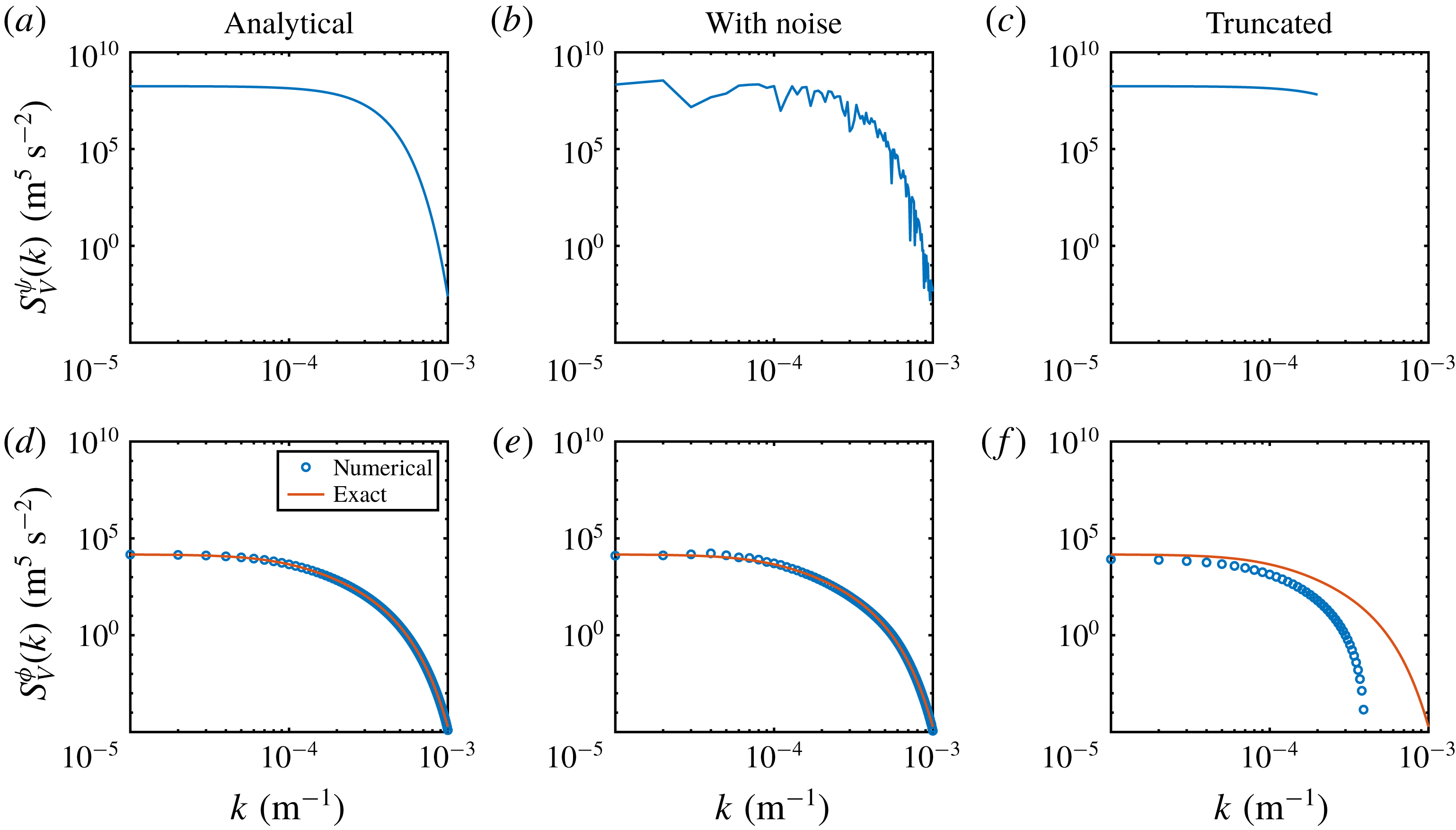
on a fine discrete grid. This we consider to be the ‘exact’ solution and we tested whether we could recover it from the method described in § 3.2. To mimic realistic conditions we also added noise to the input spectrum, or truncated it severely in wavenumber. The very encouraging results are depicted in figure 1, which indicates that our numerical method is quite robust and accurate.
Test of the numerical method from § 3.2 on the example (3.12) with
 $C=10^{4}~\text{m}^{4}~\text{s}^{-2}$
,
 $R=10^{3}~\text{m}$
,
 $f=7\times 10^{-5}~\text{s}^{-1}$
and
 $\unicode[STIX]{x1D705}_{D}=10^{-4}~\text{m}^{-1}$
. The input spectra
 $S_{V}^{\unicode[STIX]{x1D713}}(k)$
are in the upper row and the output spectra
 $S_{V}^{\unicode[STIX]{x1D719}}(k)$
are in the lower row. The left-hand column shows the outcome on a fine grid, with excellent agreement between the numerical and exact results. In the middle column strong noise was added by multiplying each gridded value of the input spectrum by a random number between zero and two. Despite this strong noise the recovery of the ageostrophic correction is remarkably good. Finally, in the right-hand column the input spectrum has been truncated at the wavenumber
 $k=2\times 10^{-4}~\text{m}^{-1}$
. This leads to the greatest error, but still reasonable recovery of the correct answer at large scales.

For reference in the next section, we note that the same algorithm can also be used to compute the kinetic energy spectrum
 $K_{\unicode[STIX]{x1D719},V}(k)$
from
 $S_{V}^{\unicode[STIX]{x1D713}}(k)$
: all that is needed is to replace
 $\widehat{L}(\unicode[STIX]{x1D705})$
by
 $0.5\unicode[STIX]{x1D705}^{2}\widehat{L}(\unicode[STIX]{x1D705})$
before the Abel transform in the final step.
4 Wave–vortex decomposition with ageostrophic correction
In this section we describe how to extend the linear wave–vortex decomposition method of BCF14 into a weakly nonlinear regime by taking into account the leading-order ageostrophic correction to the vortical, quasi-geostrophic flow. We mention again that the main shortcoming of our approach for true atmospheric data is that we can only probe the ageostrophic correction after making an assumption about a dominant vertical wavenumber, which then feeds into the definition of an effective horizontal deformation wavenumber via (2.27). Still, by varying that deformation wavenumber we can probe the likely magnitude of the ageostrophic correction for a given data set.
Starting with the observed one-dimensional spectra
 $\{S^{u}(k),S^{v}(k),S^{b}(k)\}$
of the longitudinal and transversal horizontal velocities as well as of buoyancy
 $b$
divided by the buoyancy frequency
 $N$
, we seek to decompose the total observed energy spectrum
 $$\begin{eqnarray}\displaystyle E(k)={\textstyle \frac{1}{2}}(S^{u}(k)+S^{v}(k)+S^{b}(k))=E_{W}(k)+E_{V}(k) & & \displaystyle\end{eqnarray}$$
into a sum of contributions associated with hydrostatic inertia–gravity waves on the one hand and with quasi-geostrophic vortical flows on the other. At the linear level this problem was solved by BCF14, which is our starting point.
4.1 The linear wave–vortex decomposition of BCF14
The algorithm of BCF14 consists of two steps. First, an exact Helmholtz decomposition of
 $S^{u}(k)$
and
 $S^{v}(k)$
into rotational and divergent components is performed under the sole assumption of horizontal isotropy (in particular, it is not needed to assume that the stream function and velocity potential are uncorrelated for this step to work). This utilizes a new Helmholtz decomposition algorithm developed by BCF14, which takes a particularly concise form for the sum of the two velocity spectra, i.e. for the kinetic energy spectrum
 $$\begin{eqnarray}\displaystyle K(k)={\textstyle \frac{1}{2}}(S^{u}(k)+S^{v}(k))=K_{\unicode[STIX]{x1D713}}(k)+K_{\unicode[STIX]{x1D719}}(k). & & \displaystyle\end{eqnarray}$$
This concise formula for the algorithm of BCF14 was noted by Lindborg (Reference Lindborg2015):
 $$\begin{eqnarray}\displaystyle \left.\begin{array}{@{}c@{}}\displaystyle K_{\unicode[STIX]{x1D713}}(k)=\frac{S^{v}(k)}{2}+\frac{1}{2k}\int _{k}^{\infty }[S^{v}(\unicode[STIX]{x1D70F})-S^{u}(\unicode[STIX]{x1D70F})]\,\text{d}\unicode[STIX]{x1D70F},\\[12.0pt] \displaystyle K_{\unicode[STIX]{x1D719}}(k)=\frac{S^{u}(k)}{2}-\frac{1}{2k}\int _{k}^{\infty }[S^{v}(\unicode[STIX]{x1D70F})-S^{u}(\unicode[STIX]{x1D70F})]\,\text{d}\unicode[STIX]{x1D70F}.\end{array}\right\} & & \displaystyle\end{eqnarray}$$
This kinematic decomposition holds regardless of any dynamical interpretations of the spectra. At this point the original data set has been processed to yield
 $$\begin{eqnarray}\displaystyle & \displaystyle \{S^{u}(k),S^{v}(k),S^{b}(k)\}\longmapsto \{E(k),K_{\unicode[STIX]{x1D713}}(k),K_{\unicode[STIX]{x1D719}}(k)\}. & \displaystyle\end{eqnarray}$$
The second BCF14 step uses an energy equipartition result from linear theory for uncorrelated plane inertia–gravity waves, which is
 $$\begin{eqnarray}\displaystyle E_{W}(k)=2K_{\unicode[STIX]{x1D719}}(k). & & \displaystyle\end{eqnarray}$$
Implicit in this step is that the divergent kinetic energy spectrum
 $K_{\unicode[STIX]{x1D719}}$
is attributed entirely to the waves, as is consistent with linear theory. The quasi-geostrophic, vortical energy spectrum then follows from the observed
 $E(k)$
as the residual
 $$\begin{eqnarray}\displaystyle E_{V}(k)=E(k)-E_{W}(k)=E(k)-2K_{\unicode[STIX]{x1D719}}(k). & & \displaystyle\end{eqnarray}$$
Taken together, (4.3)–(4.6) constitute the linear wave–vortex decomposition of BCF14.
4.2 Ageostrophic correction in wave–vortex decomposition
The ageostrophic correction yields a divergent kinetic energy component
 $K_{\unicode[STIX]{x1D719},V}$
such that the total vortex energy increases to
 $$\begin{eqnarray}\displaystyle E_{V}(k)=E_{\unicode[STIX]{x1D713},V}(k)+K_{\unicode[STIX]{x1D719},V}(k), & & \displaystyle\end{eqnarray}$$
where
 $E_{\unicode[STIX]{x1D713},V}$
is the quasi-geostrophic energy spectrum. For consistency, (4.5) must then be corrected to
 $$\begin{eqnarray}\displaystyle E_{W}(k)=2(K_{\unicode[STIX]{x1D719}}(k)-K_{\unicode[STIX]{x1D719},V}(k)), & & \displaystyle\end{eqnarray}$$
which isolates the part of
 $K_{\unicode[STIX]{x1D719}}$
associated with the wave field. Note that without (4.8) the ageostrophic kinetic energy would be falsely diagnosed as additional wave energy, which is a problem common to all linear decomposition schemes.
Substitution in (4.1) and rearranging yields
 $$\begin{eqnarray}\displaystyle E_{\unicode[STIX]{x1D713},V}(k)-K_{\unicode[STIX]{x1D719},V}(k)=E(k)-2K_{\unicode[STIX]{x1D719}}(k). & & \displaystyle\end{eqnarray}$$
By introducing the nonlinear ageostrophic operator
 $$\begin{eqnarray}\displaystyle K_{\unicode[STIX]{x1D719},V}(k)={\mathcal{T}}[E_{\unicode[STIX]{x1D713},V}(\cdot )](k) & & \displaystyle\end{eqnarray}$$
this becomes a nonlinear equation for
 $E_{\unicode[STIX]{x1D713},V}$
, i.e.
 $$\begin{eqnarray}\displaystyle E_{\unicode[STIX]{x1D713},V}(k)-{\mathcal{T}}[E_{\unicode[STIX]{x1D713},V}(\cdot )](k)=E(k)-2K_{\unicode[STIX]{x1D719}}(k). & & \displaystyle\end{eqnarray}$$
The right-hand side is known from the observations and the Helmholtz decomposition, so the only unknown in the equation is indeed
 $E_{\unicode[STIX]{x1D713},V}$
. The operator
 ${\mathcal{T}}[\cdot ]$
is implemented numerically based on the method developed in § 3.2. This requires an intermediate step of computing
 $S_{V}^{\unicode[STIX]{x1D713}}(k)$
from
 $E_{\unicode[STIX]{x1D713},V}(k)$
, which turns out to be (see appendix F)
 $$\begin{eqnarray}\displaystyle & \displaystyle S_{V}^{\unicode[STIX]{x1D713}}(k)=\frac{2E_{\unicode[STIX]{x1D713},V}(k)}{k^{2}+\unicode[STIX]{x1D705}_{\ast }^{2}/4}-\frac{\displaystyle \int _{k}^{\infty }2E_{\unicode[STIX]{x1D713},V}(\unicode[STIX]{x1D70F})(\unicode[STIX]{x1D70F}^{2}+\unicode[STIX]{x1D705}_{\ast }^{2}/4)^{-3/2}\,\unicode[STIX]{x1D70F}\,\text{d}\unicode[STIX]{x1D70F}}{\sqrt{k^{2}+\unicode[STIX]{x1D705}_{\ast }^{2}/4}}, & \displaystyle\end{eqnarray}$$
where
 $\unicode[STIX]{x1D705}_{\ast }^{2}/4=m_{\ast }^{2}\,f^{2}/N^{2}$
contains the adjustable parameter
 $m_{\ast }$
. The nonlinear equation (4.11) is solved iteratively for
 $E_{\unicode[STIX]{x1D713},V}(k)$
by starting with the linear decomposition of BCF14, which corresponds to
 ${\mathcal{T}}[\cdot ]=0$
in (4.11). If the iteration converges then
 $E_{V}$
and
 $E_{W}$
are finally computed from (4.7) and (4.8). Both these spectra must be non-negative by definition, which is a useful check on the validity of the theory for given data.
4.3 Test of algorithm on synthetic track data
We tested the algorithm on synthetic track data
 $S^{u}(k),S^{v}(k),S^{b}(k)$
that have been produced without any gravity waves, i.e. the underlying flow consists entirely of a quasi-geostrophic flow together with an ageostrophic correction. This is for convenience of presentation, i.e. adding some wave energy would not make any difference to the algorithm. Specifically, we assume that
 $S_{V}^{\unicode[STIX]{x1D713}}(k,l)\propto \unicode[STIX]{x1D705}^{-5.3}$
and that the dominant vertical wavelength
 $2\unicode[STIX]{x03C0}/m_{\ast }=4200~\text{m}$
. We set a mid-latitude value for
 $f$
, let
 $N=100f$
and also set the air density to a typical tropopause value. Overall, we aimed to produce synthetic data with spatial and amplitude ranges that are comparable to the actual flight-track data to be analysed subsequently.
We ran the reconstruction algorithm with three different values of
 $\unicode[STIX]{x1D705}_{R}$
, which is the value of the horizontal structure parameter
 $\unicode[STIX]{x1D705}_{\ast }$
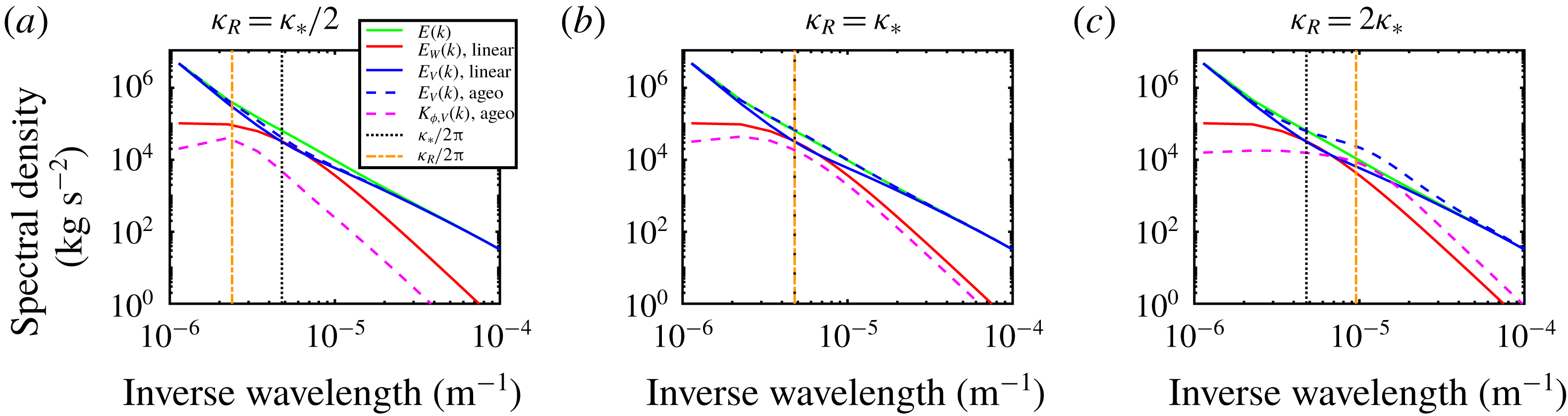
assumed in the code. The results are shown in figure 2, where the exact parameter value
 $\unicode[STIX]{x1D705}_{\ast }=2m_{\ast }\,f/N$
as well as
 $\unicode[STIX]{x1D705}_{R}$
are marked by vertical lines. The panels also show the linear wave–vortex decomposition for reference. The linear decomposition shows a clear ‘false positive’ signal of gravity wave energy near
 $\unicode[STIX]{x1D705}_{\ast }$
, where the ageostrophic kinetic energy is misinterpreted as wave energy. In figure 2(a),
 $\unicode[STIX]{x1D705}_{R}=\unicode[STIX]{x1D705}_{\ast }/2$
and consequently the ageostrophic correction is underestimated and there is only a small difference from the linear solution. In figure 2(b),
 $\unicode[STIX]{x1D705}_{R}=\unicode[STIX]{x1D705}_{\ast }$
and the reconstruction is perfect, which validates our code. In particular, the total energy is now diagnosed as vortex energy at all scales and the ageostrophic kinetic energy is precisely half of the falsely diagnosed linear wave energy, in agreement with (4.5). Finally, in figure 2(c),
 $\unicode[STIX]{x1D705}_{R}=2\unicode[STIX]{x1D705}_{\ast }$
and this excessive value produces unphysical results in which the diagnosed vortex energy exceeds the total energy. For even larger values of
 $\unicode[STIX]{x1D705}_{R}$
the algorithm fails to converge.
Test of wave–vortex decomposition on synthetic track data that have no gravity wave energy. The solid lines show the linear decomposition, which exhibits a clear false positive wave energy diagnosed at wavenumbers near
 $\unicode[STIX]{x1D705}_{\ast }$
. For small
 $\unicode[STIX]{x1D705}_{R}$
(a) the code essentially repeats the linear solution. In (b),
 $\unicode[STIX]{x1D705}_{R}=\unicode[STIX]{x1D705}_{\ast }$
and the code recovers the correct answer exactly. Finally, in (c), an excessive value of
 $\unicode[STIX]{x1D705}_{R}$
leads to unphysical results.

Overall, this example validates our code and illustrates that when probing actual data the usable range of
 $\unicode[STIX]{x1D705}_{R}$
goes from zero up to a data-dependent value where the decomposition becomes unphysical. The sensitivity of the decomposition across this usable range of
 $\unicode[STIX]{x1D705}_{R}$
then gives an indication of the robustness of the linear decomposition result against a possible ageostrophic correction.
5 Application to MOZAIC and START08 atmospheric data sets
We have applied our ageostrophic wave–vortex decomposition method to atmospheric flight-track data collected near the mid-latitude tropopause. Specifically, we looked at the well-studied data from the MOZAIC and START08 campaigns (Nastrom & Gage Reference Nastrom and Gage1985; Zhang et al. Reference Zhang, Wei, Zhang, Bowman, Pan, Atlas and Wofsy2015) and followed closely the diagnostic procedures in Callies et al. (Reference Callies, Bühler and Ferrari2016), where the same sets were analysed using the linear wave–vortex decomposition method.
5.1 Data preparation methods
For details we refer to Callies et al. (Reference Callies, Bühler and Ferrari2016). Briefly, the tracks were classified into upper tropospheric and lower stratospheric tracks based on the stratification along the track, which was available from re-analysis data. The altitude along each segment identified was nearly constant and a total of 15 tropospheric segments and 65 stratospheric segments were identified in the START08 project data whilst 2752 tropospheric segments and 4681 stratospheric segments were identified in the MOZAIC data. The spectra processed from the MOZAIC project ranged from 10 to 1000 km in wavelength and the spectra processed from the START08 project ranged from 1 to 100 km in wavelength. So START08 can be viewed as extending the MOZAIC data to smaller scales. We patched the spectra from both projects together so that we can analyse a set of spectra whose wavelength ranges from 1 to 1000 km. At the scales where the spectra from the two projects overlap, we weighted each set by the number of the segments identified in each project. Weighting the spectra by number of segments de facto favours the MOZAIC data over the START08 data in the overlapping scales. This could be problematic, especially for the tropospheric
 $S^{u}(k)$
spectrum, because, as noted in Callies et al. (Reference Callies, Bühler and Ferrari2016), a significant mismatch of the tropospheric
 $S^{u}(k)$
spectra between the two projects is observed.
The basic density around the tropopause decays with altitude, so in order to avoid the spectra from being biased towards the high-altitude tracks, the spectra at each segment are weighted by the along-track density before evaluating the covariance functions. Our ageostrophic algorithm does not use density-weighted spectra, so we divide the spectra by typical densities for stratospheric and tropospheric tracks, which we chose to be
 $0.34$
and
 $0.39$
in standard units. To keep the units consistent with Callies et al. (Reference Callies, Bühler and Ferrari2016), we multiply the diagnosed spectra with the mean densities before plotting the results.
5.2 Choice of
$\unicode[STIX]{x1D705}_{R}$
and decomposition results

We tried different values for the effective deformation wavenumber
 $\unicode[STIX]{x1D705}_{R}$
in order to probe the data for the likely size of the ageostrophic corrections in the decomposition. Following (2.27),
 $\unicode[STIX]{x1D705}_{R}$
and the implied dominant vertical wavenumber
 $m$
are linked by
 $\unicode[STIX]{x1D705}_{R}=2mf/N$
. At the lower end, the first baroclinic mode in the troposphere has vertical wavenumber
 $m_{1}=\unicode[STIX]{x03C0}/H$
, where
 $H$
is the height of the tropopause, so
 $m_{1}\approx 3\times 10^{-4}~\text{m}^{-1}$
. Using a standard value of
 $f/N=100$
this yields a corresponding mode-one value for
 $\unicode[STIX]{x1D705}_{R}$
of approximately
 $6\times 10^{-6}~\text{m}^{-1}$
. We used this typical synoptic-scale value as a suitable lower bound for
 $\unicode[STIX]{x1D705}_{R}$
. There is no obvious upper bound on
 $\unicode[STIX]{x1D705}_{R}$
, but in practice the algorithm produces unphysical results when
 $\unicode[STIX]{x1D705}_{R}$
is too large, similar to what was encountered in the synthetic examples in § 4.3. We found empirically that for the tropospheric data set the algorithm worked up to values of
 $\unicode[STIX]{x1D705}_{R}$
corresponding to the fourth baroclinic mode, but that it delivered unphysical results thereafter. There was much more leeway for the stratospheric data, but in order to have a consistent method, we restricted ourselves to the tropospheric range for
 $\unicode[STIX]{x1D705}_{R}$
. So, basically, our trial values for
 $\unicode[STIX]{x1D705}_{R}$
ranged from the synoptic to the larger end of the mesoscale.
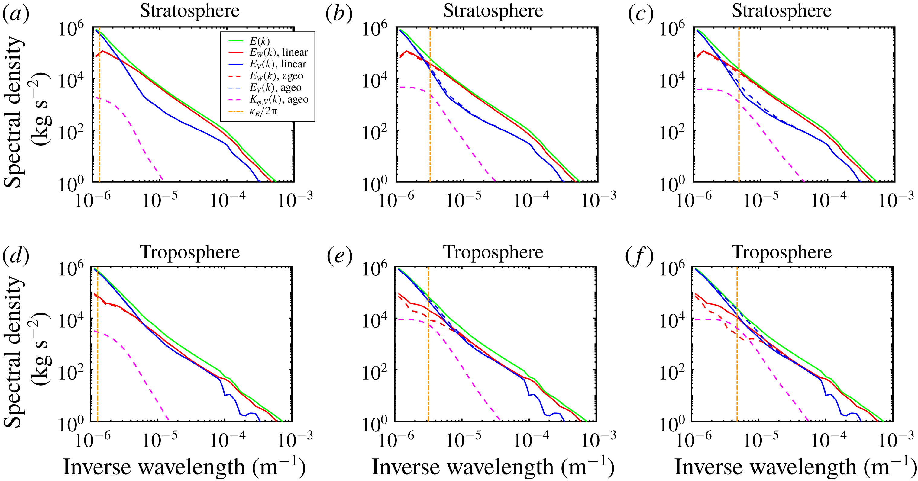
The results of running the algorithm are displayed in figure 3. The three values of
 $\unicode[STIX]{x1D705}_{R}$
correspond, roughly, to the first, third and fourth baroclinic modes in the troposphere. Figure 3(a–c) shows the stratospheric data decomposition and here we find that the ageostrophic correction to the wave–vortex decomposition is pretty much negligible for the range of values of
 $\unicode[STIX]{x1D705}_{R}$
that we considered. This suggests that the stratospheric data are well approximated by the linear decomposition method of Callies et al. (Reference Callies, Bühler and Ferrari2016) and that their main conclusion, namely that the wave energy dominates at all scales below a few hundred kilometres, is robust. A different story unfolds for the tropospheric data in figure 3(d–f). Here only figure 3(d), which corresponds to ageostrophic corrections associated with the first baroclinic mode, shows negligible ageostrophic corrections at all scales. Figure 3(e,f), on the other hand, shows significant ageostrophic corrections for horizontal wavenumbers near
 $\unicode[STIX]{x1D705}_{R}$
. These corrections always reduce the amount of energy attributed to the waves in that region. Indeed, in figure 3(f) essentially all the energy near
 $\unicode[STIX]{x1D705}_{R}$
is now attributed to the vortical flow, whereas the linear decomposition method indicated equipartition between wave and vortex energy. Of course, for this large value of
 $\unicode[STIX]{x1D705}_{R}$
the algorithm is close to producing unphysical results, which as we know from the synthetic examples manifests itself as vortex energy exceeding the observed energy.
Ageostrophic decomposition applied to atmospheric flight-track data in (a–c) the lower stratosphere and (d–f) the upper troposphere. (The plotted spectra have been divided by
 $2\unicode[STIX]{x03C0}$
to conform with the scaling of Callies et al. (Reference Callies, Bühler and Ferrari2016).) Three values of
 $\unicode[STIX]{x1D705}_{R}$
have been used: (a,d)
 $\unicode[STIX]{x1D705}_{R}=8\times 10^{-6}~\text{m}^{-1}$
, (b,e)
 $\unicode[STIX]{x1D705}_{R}=2\times 10^{-5}~\text{m}^{-1}$
and (c,f)
 $\unicode[STIX]{x1D705}_{R}=3\times 10^{-5}~\text{m}^{-1}$
.

So it is hard to decide whether the behaviour in figure 3(f) is physical or simply an artifact caused by assuming too large a value of
 $\unicode[STIX]{x1D705}_{R}$
. What is clear, however, is that the tropospheric data are not as robust as the stratospheric data when considering ageostrophic corrections. Notably, the decomposition results at scales below
 $\unicode[STIX]{x1D705}_{R}$
remain virtually unchanged in all cases, so at the moment our method, which can only probe a single dominant vertical wavenumber, is too blunt to investigate the full range of the horizontal energy spectra, at least in the troposphere. There, the wave energy still dominates over the vortex energy at inverse wavelengths smaller than
 $4\times 10^{-6}~\text{m}^{-1}$
and the rough equipartition between wave and vortex energy observed for MOZAIC data in Callies et al. (Reference Callies, Bühler and Ferrari2016) at mesocales still persists, although its range is narrowed slightly. A simple physical explanation for this apparent equipartition, and why it is not observed in the START08 data, remains elusive.
6 Concluding remarks
In the first half of our paper we derived what one might call the power spectral version of the omega equation, which for the shallow-water system was given in the various equivalent forms (2.15), (2.17), (2.19), e.g.
 $$\begin{eqnarray}\displaystyle S_{V}^{\unicode[STIX]{x1D719}}(\boldsymbol{k})=\left(\frac{\unicode[STIX]{x1D705}_{D}^{2}/f}{\unicode[STIX]{x1D705}^{2}(\unicode[STIX]{x1D705}^{2}+\unicode[STIX]{x1D705}_{D}^{2})}\right)^{2}\frac{1}{2L^{2}}\,\mathop{\sum }_{\boldsymbol{k}=\boldsymbol{k}_{1}+\boldsymbol{k}_{2}}\,S_{V}^{\unicode[STIX]{x1D713}}(\boldsymbol{k}_{1})S_{V}^{\unicode[STIX]{x1D713}}(\boldsymbol{k}_{2})\,|(\unicode[STIX]{x1D705}_{2}^{2}-\unicode[STIX]{x1D705}_{1}^{2})(\boldsymbol{k}_{1}\times \boldsymbol{k}_{2})|^{2}. & & \displaystyle\end{eqnarray}$$
The corresponding three-dimensional version for the Boussinesq system is (C 1) in appendix C. The only simplifying assumption that went into the derivation of these power spectral omega equations is that the Fourier components of the quasi-geostrophic stream function are mutually independent, which includes the common cases of Gaussian random functions or the random phase approximations. So within these limitations the equations are quite general, and can for instance be used to estimate ageostrophic effects in anisotropic flow situations when the power spectrum
 $S_{V}^{\unicode[STIX]{x1D713}}$
is known. This could be useful in a variety of situations where the statistics of the ageostrophic correction are of interest (e.g. Kafiabad & Bartello Reference Kafiabad and Bartello2016; Kafiabad, Savva & Vanneste Reference Kafiabad, Savva and Vanneste2019). For example, it would be interesting to compare our solution of the statistical omega equation to the balanced ageostrophic energy spectra computed by other numerical means in Kafiabad & Bartello (Reference Kafiabad and Bartello2016).
In the second half of our paper we used these equations to extend a wave–vortex decomposition method for one-dimensional spectra, but under the additional assumption of horizontal isotropy. Here we encountered two problems, one expected and one unexpected. First, the three-dimensional power spectral omega equation obviously requires knowledge of the vertical structure, which is not available from the horizontal track data. Ideally, one should use Charney’s three-dimensional isotropy assumption for the quasi-geostrophic stream function (i.e. that its power spectrum is a function only of
 $k^{2}+l^{2}+f^{2}m^{2}/N^{2}$
) in order to solve the three-dimensional power spectral omega equation, but we were not able to do that. Instead we used the primitive device of allowing only a monochromatic structure in the vertical, with a single dominant wavenumber
 $m_{\ast }$
. As discussed, this obviously handicapped the application of our method to real data. The second problem was unexpected, namely that it was very hard to evaluate an equation such as (2.15) when only one-dimensional spectra are observed. This was because these one-dimensional spectra are related to the two-dimensional spectra by the Abel forward transform (3.6), and undoing this step by an Abel inverse transform turned out to be so unstable that it was of no use in a practical situation. This led to the seemingly cumbersome, but ultimately successful, algorithm described in § 3.2.
This allowed us to incorporate the ageostrophic correction into the linear wave–vortex decomposition of BCF14, rendering that decomposition method weakly nonlinear (in the sense of low Rossby number for the relevant scales), to be solved by the nonlinear iteration of (4.11). The key difference from the linear scheme was that now ageostrophic divergent kinetic energy could be recognized as such, and was not diagnosed mistakenly for wave energy. Application to atmospheric flight-track data near the tropopause showed that the lower stratospheric spectra were robust under this ageostrophic correction, but that this was much less clear for the upper tropospheric tracks, where some of the decomposition results between the synoptic and the mesoscales were sensitive to the ageostrophic correction we computed. Of course, our results were limited in practice by the artificial assumption of a single vertical wavenumber. So, despite considerable effort, the final word on the interpretation of the upper tropospheric data is not yet out. Given the discrepancies between tropospheric START08 and MOZAIC data that were noted in Callies et al. (Reference Callies, Bühler and Ferrari2016), it seems likely that more data and more sophisticated analysis techniques beyond the assumptions of a single vertical mode for the balanced flow will be needed to settle this question.
The other assumptions made throughout the work, such as horizontal isotropy, uncorrelated wave and vortex motion and independent Fourier modes, are of course also questionable and further modifications of the wave–vortex decomposition method are yet to be explored. In particular, in Bühler et al. (Reference Bühler, Callies and Ferrari2014), the horizontal anisotropy in the data taken at Gulf Stream renders non-physical outcomes in the wave–vortex decomposition, and a solution is proposed in Bühler et al. (Reference Bühler, Kuang and Tabak2017), which brings up a linear wave–vortex decomposition algorithm applicable to data with anisotropy. It should be possible to formulate a statistical omega equation in this situation as well.
Finally, it was pointed out to us by a referee that a purely wavelike flow would presumably project nonlinearly onto the quasi-geostrophic mode and therefore would produce a false positive diagnosis of balanced flow energy in any linear wave–vortex decomposition scheme. This is the flip side of our present consideration of a false positive diagnosis of wave energy, which could for example be relevant to the slow wave-induced mean flows studied in Bühler & Holmes-Cerfon (Reference Bühler and Holmes-Cerfon2009) and Holmes-Cerfon, Bühler & Ferrari (Reference Holmes-Cerfon, Bühler and Ferrari2011).
Acknowledgements
We are indebted to Jörn Callies for stimulating scientific discussions and invaluable help with the MOZAIC and START08 data. H.W. thanks Michael Lever for numerous discussions, especially about the Hankel transform. The comments and suggestions of three referees helped improve our manuscript. We gratefully acknowledge financial support from United States National Science Foundation grants DMS-1813891, DMS-1312159 and DMS-1516324 as well as from Office of Naval Research grants N00014-15-1-2355 and N00014-19-1-2407.
Appendix A. Example with correlation between
$\unicode[STIX]{x1D719}_{V}$
and
$\unicode[STIX]{x1D713}_{V}$


Consider the random stream function
 $$\begin{eqnarray}\displaystyle \widehat{\unicode[STIX]{x1D713}}_{V}(k,l)=L\sqrt{S_{V}^{\unicode[STIX]{x1D713}}(k,l)}\text{e}^{-\text{i}(ka+lb)}, & & \displaystyle\end{eqnarray}$$
where
 $a$
and
 $b$
are independent uniformly distributed random variables taking values in
 $[0,L]$
. By inspection, this achieves the prescribed power spectrum and the stream function consists of a fixed pattern that is randomly shifted by the vector
 $(a,b)$
, thereby making the stream function homogeneous in space. Hence its Fourier components are uncorrelated, but they are not independent. Indeed, if we compute
 $\widehat{\unicode[STIX]{x1D719}}_{V}$
from (2.12), we obtain the non-zero cross-spectrum
 $$\begin{eqnarray}\displaystyle \overline{\widehat{\unicode[STIX]{x1D713}}_{V}^{\ast }\widehat{\unicode[STIX]{x1D719}}_{V}}=L\mathop{\sum }_{\boldsymbol{k}_{1}+\boldsymbol{k}_{2}=\boldsymbol{k}}\frac{\unicode[STIX]{x1D705}_{D}^{2}(k_{1}k_{2}^{2}l_{2}+k_{1}l_{2}^{3}-l_{1}k_{2}^{3}-l_{1}l_{2}^{2}k_{2})}{f(k^{2}+l^{2})(k^{2}+l^{2}+\unicode[STIX]{x1D705}_{D}^{2})}\sqrt{S_{V}^{\unicode[STIX]{x1D713}}(\boldsymbol{k})S_{V}^{\unicode[STIX]{x1D713}}(\boldsymbol{k}_{1})S_{V}^{\unicode[STIX]{x1D713}}(\boldsymbol{k}_{2})}. & & \displaystyle\end{eqnarray}$$
Appendix B. Pseudospectral evaluation of (2.15)
The expression (2.15) can be expanded as
 $$\begin{eqnarray}\displaystyle S_{V}^{\unicode[STIX]{x1D719}}(k,l) & = & \displaystyle \left(\frac{\unicode[STIX]{x1D705}_{D}^{2}/f}{\unicode[STIX]{x1D705}^{2}(k^{2}+l^{2}+\unicode[STIX]{x1D705}_{D}^{2})}\right)^{2}\frac{1}{L^{2}}\mathop{\sum }_{\boldsymbol{k}=\boldsymbol{k}_{1}+\boldsymbol{k}_{2}} (-k_{1}^{4}k_{2}^{2}l_{2}^{2}-k_{1}^{4}l_{2}^{4}+2k_{1}^{3}l_{1}k_{2}^{3}l_{2}\nonumber\\ \displaystyle & & \displaystyle \text{}+2k_{1}^{3}l_{1}k_{2}l_{2}^{3}-k_{1}^{2}l_{1}^{2}k_{2}^{4}-2k_{1}^{2}l_{1}^{2}k_{2}^{2}l_{2}^{2}-k_{1}^{2}l_{1}^{2}l_{2}^{4}+2k_{1}l_{1}^{3}k_{2}^{3}l_{2}+2k_{1}l_{1}^{3}k_{2}l_{2}^{3}\nonumber\\ \displaystyle & & \displaystyle \text{}-l_{1}^{4}k_{2}^{4}-l_{1}^{4}k_{2}^{2}l_{2}^{2}+k_{1}^{2}k_{2}^{4}l_{2}^{2}+2k_{1}^{2}k_{2}^{2}l_{2}^{4}+k_{1}^{2}l_{2}^{6}-2k_{1}l_{1}k_{2}^{5}l_{2}-4k_{1}l_{1}k_{2}^{3}l_{2}^{3}\nonumber\\ \displaystyle & & \displaystyle \text{}-2k_{1}l_{1}k_{2}l_{2}^{5}+l_{1}^{2}k_{2}^{6}+2l_{1}^{2}k_{2}^{4}l_{2}^{2}+l_{1}^{2}k_{2}^{2}l_{2}^{4} )S_{V}^{\unicode[STIX]{x1D713}}(k_{1},l_{1})S_{V}^{\unicode[STIX]{x1D713}}(k_{2},l_{2}).\end{eqnarray}$$
Taking the first term, the Fourier convolution theorem implies the identity
 $$\begin{eqnarray}\displaystyle \frac{1}{L^{2}}\mathop{\sum }_{\boldsymbol{k}=\boldsymbol{k}_{1}+\boldsymbol{k}_{2}}(k_{1}^{4}k_{2}^{2}l_{2}^{2})S_{V}^{\unicode[STIX]{x1D713}}(k_{1},l_{1})S_{V}^{\unicode[STIX]{x1D713}}(k_{2},l_{2})={\mathcal{F}}_{2}\left[\frac{\unicode[STIX]{x2202}^{4}C_{V}^{\unicode[STIX]{x1D713}}(x,y)}{\unicode[STIX]{x2202}x^{4}}\frac{\unicode[STIX]{x2202}^{4}C_{V}^{\unicode[STIX]{x1D713}}(x,y)}{\unicode[STIX]{x2202}x^{2}\unicode[STIX]{x2202}y^{2}}\right]. & & \displaystyle\end{eqnarray}$$
This uses the Fourier transform defined in (3.4). Any such term can therefore be evaluated quickly using the pseudospectral method. The other
 $19$
terms on the right-hand side of (B 1) can be treated in the same way.
Appendix C. Power spectral three-dimensional omega equation
Essentially the same steps from the two-dimensional case in § 2.2 can also be applied to the three-dimensional Boussinesq equations. Hence, if two three-dimensional fields
 $\unicode[STIX]{x1D713}_{V}$
and
 $\unicode[STIX]{x1D719}_{V}$
are linked via (2.21), extending the definitions of power spectra to three dimensions with the homogeneity assumption, we can also show that if
 $\widehat{\unicode[STIX]{x1D713}}_{V}$
are mutually independent at different wavenumbers except when the reality condition enforces, then
 $\unicode[STIX]{x1D713}_{V}$
and
 $\unicode[STIX]{x1D719}_{V}$
are uncorrelated and
 $$\begin{eqnarray}\displaystyle S_{V}^{\unicode[STIX]{x1D719}}(k,l,m) & = & \displaystyle \left(\frac{f/N^{2}}{\unicode[STIX]{x1D705}^{2}\left(k^{2}+l^{2}+{\displaystyle \frac{f^{2}}{N^{2}}}m^{2}\right)}\right)^{2}\frac{1}{L^{2}H}\mathop{\sum }_{\boldsymbol{k}=\boldsymbol{k}_{1}+\boldsymbol{k}_{2}}\nonumber\\ \displaystyle & & \displaystyle \text{} (((k^{2}+l^{2})(k_{1}m_{2}^{2}l_{2}-l_{1}m_{2}^{2}k_{2})-m^{2}(k_{1}k_{2}^{2}l_{2}+k_{1}l_{2}^{3}-l_{1}k_{2}^{3}-l_{1}l_{2}^{2}k_{2}))^{2}\nonumber\\ \displaystyle & & \displaystyle \text{}+(k^{2}+l^{2})^{2}(k_{1}m_{2}^{2}l_{2}-l_{1}m_{2}^{2}k_{2})(k_{2}m_{1}^{2}l_{1}-l_{2}m_{1}^{2}k_{1})\nonumber\\ \displaystyle & & \displaystyle \text{}-m^{4}(k_{1}k_{2}^{2}l_{2}+k_{1}l_{2}^{3}-l_{1}k_{2}^{3}-l_{1}l_{2}^{2}k_{2})(k_{2}k_{1}^{2}l_{1}+k_{2}l_{1}^{3}-l_{2}k_{1}^{3}-l_{2}l_{1}^{2}k_{1}))\nonumber\\ \displaystyle & & \displaystyle \text{}\times S_{V}^{\unicode[STIX]{x1D713}}(k_{1},l_{1},m_{1})S_{V}^{\unicode[STIX]{x1D713}}(k_{2},l_{2},m_{2}),\end{eqnarray}$$
where
 $H$
is the periodicity length in the vertical coordinate
 $z$
.
Appendix D. Illustration of unstable Abel inverse transform
The Abel transform of a radially symmetric function
 $f(r)$
in the
 $xy$
-plane is
 $$\begin{eqnarray}\displaystyle & \displaystyle g(x)=\int _{-\infty }^{+\infty }f(r)\,\text{d}y. & \displaystyle\end{eqnarray}$$
In principle, the even function
 $g(x)=g(-x)$
can be exactly inverted to yield
 $f(r)$
, but in practice this process is unstable. To illustrate this we note that if
 $k>0$
and
 $$\begin{eqnarray}\displaystyle & \displaystyle f(r)=J_{0}(kr)\quad \text{then }g(x)=\frac{2}{k}\cos (kx). & \displaystyle\end{eqnarray}$$
The division by
 $k$
indicates how high-frequency oscillations in
 $f(r)$
are damped and produce only small-amplitude oscillations in
 $g(x)$
. This makes obvious that the inversion will be unstable to small-amplitude high-frequency noise. For example, if
 $\unicode[STIX]{x1D716}\ll 1$
and
 $$\begin{eqnarray}\displaystyle & \displaystyle g(x)=\frac{2}{k}\cos (kx)+2\unicode[STIX]{x1D716}\cos (x/\unicode[STIX]{x1D716})\quad \text{then }f(r)=J_{0}(kr)+J_{0}(r/\unicode[STIX]{x1D716}). & \displaystyle\end{eqnarray}$$
Hence the Abel inverse transform is completely wrong at leading order.
Appendix E. Details of the numerics of the one-dimensional calculation
The function
 $g(r)$
is numerically evaluated as the inverse Fourier series of
 $S_{V}^{\unicode[STIX]{x1D713}}(k)$
on a discrete grid. We have been assuming that
 $S_{V}^{\unicode[STIX]{x1D713}}(k)$
is zero beyond some cut-off wavenumber, so if we zero-pad
 $S_{V}^{\unicode[STIX]{x1D713}}(k)$
onto a larger spectral grid that has
 $M>N$
grid points spaced at
 $\unicode[STIX]{x0394}k$
, the inverse Fourier series expansion of the zero-padded
 $S_{V}^{\unicode[STIX]{x1D713}}(k)$
will give us
 $g(r)$
at the finer grid with
 $(M/2+1)$
grid points spaced at
 $2\unicode[STIX]{x03C0}/(M\unicode[STIX]{x0394}k)$
, spanning from
 $0$
to
 $N\unicode[STIX]{x0394}x$
. This is an effective way to interpolate
 $g(r)$
onto a finer grid so that the numerical evaluations on its derivatives can be improved. We then conduct the pseudospectral calculation and evaluate the expression (3.10) at all the
 $M$
points on the finer grid. The larger
 $M$
is, the more accurate our outcome should be. We then conduct the calculations with increasing
 $M$
and compare the results; if the results do not change significantly when
 $M$
is doubled, we would stop increasing
 $M$
and take the outcome as the settled evaluation of (3.10). Empirically, for the application in this project, we find
 $M=8N$
to be an adequate stopping value.
For the Hankel transform (3.11) we used code from the Matlab File Exchange. In doing so we encountered one numerical problem: the value of
 $\widehat{G}(0)$
was not equal to zero, which can be catastrophic if we multiply
 $\widehat{G}(\unicode[STIX]{x1D705})$
with an
 $\widehat{L}(\unicode[STIX]{x1D705})$
that blows up at
 $\unicode[STIX]{x1D705}=0$
. In the applications presented in this paper, the magnitude of
 $\widehat{G}(0)$
is always smaller than 1 % of the average value
 $\widehat{G}(\unicode[STIX]{x1D705})$
, so we manually subtracted
 $\widehat{G}(0)$
from
 $\widehat{G}(\unicode[STIX]{x1D705})$
, as the general shape of
 $\widehat{G}(\unicode[STIX]{x1D705})$
will not be affected significantly. We hence apply this trick to ensure that
 $\widehat{G}(\unicode[STIX]{x1D705})$
is numerically zero at the origin. In some cases, after this subtraction, small negative values at a few grid points would emerge, which are non-physical due to the non-negativeness of
 $S_{V}^{\unicode[STIX]{x1D719}}$
; we suppress those small negative values to zero, which again did not affect the general shape of
 $\widehat{G}(\unicode[STIX]{x1D705})$
.
The last step is to evaluate the numerical integration (3.6). To treat the divergence of the integrand at
 $\unicode[STIX]{x1D705}=k$
, we regard the integral as
 $$\begin{eqnarray}\displaystyle & \displaystyle S_{V}^{\unicode[STIX]{x1D719}}(k)=\frac{1}{\unicode[STIX]{x03C0}}\left(\int _{k}^{k+\unicode[STIX]{x0394}k}\frac{{\hat{h}}(\unicode[STIX]{x1D705})\unicode[STIX]{x1D705}}{\sqrt{\unicode[STIX]{x1D705}^{2}-k^{2}}}\,\text{d}\unicode[STIX]{x1D705}+\int _{k+\unicode[STIX]{x0394}k}^{\infty }\frac{{\hat{h}}(\unicode[STIX]{x1D705})\unicode[STIX]{x1D705}}{\sqrt{\unicode[STIX]{x1D705}^{2}-k^{2}}}\,\text{d}\unicode[STIX]{x1D705}\right),\quad k\geqslant 0. & \displaystyle\end{eqnarray}$$
The second integral in (E 1) can be directly evaluated by the trapezoidal rule. From integration by parts, the first integral in (E 1) is
 $$\begin{eqnarray}\displaystyle & \displaystyle \frac{1}{\unicode[STIX]{x03C0}}\left({\hat{h}}(k)\sqrt{2k\unicode[STIX]{x0394}k+\unicode[STIX]{x0394}k^{2}}-\int _{k}^{k+\unicode[STIX]{x0394}k}{\hat{h}}^{\prime }(\unicode[STIX]{x1D705})\sqrt{\unicode[STIX]{x1D705}^{2}-k^{2}}\,\text{d}\unicode[STIX]{x1D705}\right), & \displaystyle\end{eqnarray}$$
and as long as
 ${\hat{h}}^{\prime }(\unicode[STIX]{x1D705})$
does not blow up near
 $\unicode[STIX]{x1D705}=k$
, the term
 $\int _{k}^{k+\unicode[STIX]{x0394}k}{\hat{h}}^{\prime }(\unicode[STIX]{x1D705})\sqrt{\unicode[STIX]{x1D705}^{2}-k^{2}}\,\text{d}\unicode[STIX]{x1D705}$
can be ignored compared with
 ${\hat{h}}(k)\sqrt{2k\unicode[STIX]{x0394}k+\unicode[STIX]{x0394}k^{2}}$
. Thus, all the components in (E 1) can be calculated numerically. This approach to evaluate (3.6) preserves the non-negativeness of
 ${\hat{h}}(\unicode[STIX]{x1D705})$
.
Appendix F. Derivation of (4.12)
The task is to compute
 $S_{V}^{\unicode[STIX]{x1D713}}(k)$
from the quasi-geostrophic energy spectrum
 $$\begin{eqnarray}\displaystyle & \displaystyle E_{\unicode[STIX]{x1D713},V}(k)={\textstyle \frac{1}{2}}(S_{\unicode[STIX]{x1D713},V}^{u}(k)+S_{\unicode[STIX]{x1D713},V}^{v}(k)+S_{\unicode[STIX]{x1D713},V}^{b}(k)). & \displaystyle\end{eqnarray}$$
Quasi-geostrophic theory, horizontal isotropy and the assumption of a single vertical wavenumber
 $m_{\ast }$
imply the following relations:
 $$\begin{eqnarray}\displaystyle & \displaystyle S_{\unicode[STIX]{x1D713},V}^{v}(k)=-k\frac{\text{d}}{\text{d}k}S_{\unicode[STIX]{x1D713},V}^{u}(k)=k^{2}S_{V}^{\unicode[STIX]{x1D713}}(k)\quad \text{and}\quad S_{\unicode[STIX]{x1D713},V}^{b}(k)=\frac{m_{\ast }^{2}\,f^{2}}{N^{2}}S_{V}^{\unicode[STIX]{x1D713}}(k). & \displaystyle\end{eqnarray}$$
Hence, differentiating (F 1) with respect to
 $k$
yields the ordinary differential equation
 $$\begin{eqnarray}\displaystyle & \displaystyle 2\frac{\text{d}}{\text{d}k}E_{\unicode[STIX]{x1D713},V}(k)=kS_{V}^{\unicode[STIX]{x1D713}}(k)+\left(k^{2}+\frac{m_{\ast }^{2}\,f^{2}}{N^{2}}\right)\frac{\text{d}}{\text{d}k}S_{V}^{\unicode[STIX]{x1D713}}(k). & \displaystyle\end{eqnarray}$$
The general solution of (F 3) is
 $$\begin{eqnarray}\displaystyle & \displaystyle S_{V}^{\unicode[STIX]{x1D713}}(k)=\frac{2E_{\unicode[STIX]{x1D713},V}(k)(k^{2}+\unicode[STIX]{x1D705}_{\ast }^{2}/4)^{-1/2}+\displaystyle \int _{0}^{k}2E_{\unicode[STIX]{x1D713},V}(\unicode[STIX]{x1D70F})(\unicode[STIX]{x1D70F}^{2}+\unicode[STIX]{x1D705}_{\ast }^{2}/4)^{-3/2}\unicode[STIX]{x1D70F}\,\text{d}\unicode[STIX]{x1D70F}-A}{\sqrt{k^{2}+\unicode[STIX]{x1D705}_{\ast }^{2}/4}}, & \displaystyle\end{eqnarray}$$
where
 $\unicode[STIX]{x1D705}_{\ast }^{2}/4=m_{\ast }^{2}\,f^{2}/N^{2}$
and
 $A$
is a constant of integration, which is fixed by demanding that
 $S_{V}^{\unicode[STIX]{x1D713}}(k)$
is integrable, i.e. that the stream function has a finite variance. This leads to
 $$\begin{eqnarray}\displaystyle & \displaystyle A=\int _{0}^{\infty }2E_{\unicode[STIX]{x1D713},V}(\unicode[STIX]{x1D70F})(\unicode[STIX]{x1D70F}^{2}+\unicode[STIX]{x1D705}_{\ast }^{2}/4)^{-3/2}\unicode[STIX]{x1D70F}\,\text{d}\unicode[STIX]{x1D70F}, & \displaystyle\end{eqnarray}$$
and therefore
 $$\begin{eqnarray}\displaystyle & \displaystyle S_{V}^{\unicode[STIX]{x1D713}}(k)=\frac{2E_{\unicode[STIX]{x1D713},V}(k)}{k^{2}+\unicode[STIX]{x1D705}_{\ast }^{2}/4}-\frac{\displaystyle \int _{k}^{\infty }2E_{\unicode[STIX]{x1D713},V}(\unicode[STIX]{x1D70F})(\unicode[STIX]{x1D70F}^{2}+\unicode[STIX]{x1D705}_{\ast }^{2}/4)^{-3/2}\,\unicode[STIX]{x1D70F}\,\text{d}\unicode[STIX]{x1D70F}}{\sqrt{k^{2}+\unicode[STIX]{x1D705}_{\ast }^{2}/4}} & \displaystyle\end{eqnarray}$$
is the desired relation.