1 Introduction
Laminar flow around arbitrarily shaped bodies is a classical problem in fluid mechanics. Such arbitrarily shaped bodies can be aerodynamically classified into: (i) bluff body and (ii) slender body. If the drag force experienced by the body is largely due to pressure, then it is defined as a bluff body. The famous example of a bluff body is a circular cylinder. On the other hand, the drag force on a slender body is predominantly due to skin friction. A well-known example for a slender body is a flat plate placed along the flow direction. Though flow past various shaped bodies is widely studied, most of the previous studies are on flow around canonical bodies such as the circular and square cylinders. In recent years, studies on the flow past non-canonical bodies are gaining interest due to their novel wake characteristics. One such unorthodox geometry is an elliptic cylinder. Flow past the elliptic cylinder is influenced by parameters such as axis ratio (
 $AR$
, which is defined as the ratio of semi-minor axis (
 $b$
) to semi-major axis (
 $a$
)), and angle of attack (AOA) besides the usual flow parameter, the Reynolds number (
 $Re$
). A circular cylinder is a form of elliptic cylinder with
 $AR=1.0$
.
The literature on elliptic cylinder wakes reveals that the most of the previous studies are on the flow due to an impulsively started elliptic cylinder (Taneda Reference Taneda1972), for a higher Reynolds number (Mittal & Balachandar Reference Mittal and Balachandar1996) or for a steady flow (Faruquee et al.
Reference Faruquee, Ting, Fartaj, Barron and Carrivaeu2007). For the problem considered in this paper, the previous works focused predominately on the classification of flow pattern with respect to vorticity contour. For instance, the numerical study by Park, Park & Hyun (Reference Park, Park and Hyun1989) identified five different regimes of distinguished flow characteristics, while six different types of vorticity patterns were observed by Johnson, Thompson & Hourigan (Reference Johnson, Thompson and Hourigan2001) and Johnson, Thompson & Hourigan (Reference Johnson, Thompson and Hourigan2004) for varying
 $Re$
in their numerical studies. Low-frequency unsteadiness in the far wake is an another aspect in the elliptic cylinder wakes which was first studied by Johnson et al. (Reference Johnson, Thompson and Hourigan2004). Drag coefficients and Strouhal numbers were computed experimentally by Radi et al. (Reference Radi, Thompson, Sheridan and Hourigan2013), and these values were later verified by Thompson et al. (Reference Thompson, Radi, Rao, Sheridan and Hourigan2014) for both two-dimensional (2-D) and 3-D simulations. The onset of laminar separation and vortex shedding in an elliptic cylinder was studied by Paul et al. (Reference Paul, Arul Prakash and Vengadesan2014b
), while the critical
 $Re$
at which the flow goes from 2-D to 3-D was reported by Thompson et al. (Reference Thompson, Radi, Rao, Sheridan and Hourigan2014).
Only a very few articles have been published on the analysis of thermal wakes of elliptic cylinders. Experimental studies on forced convective heat transfer from elliptic cylinders proved that
 $Nu_{avg}$
increases with
 $Re$
and
 $AR$
, but decreases with AOA (Ota et al.
Reference Ota, Aiba, Tsuruta and Kaga1983). There are some numerical studies of convective heat transfer from elliptic cylinders. However, they were carried out for a very low Reynolds number (D’Alessio & Dennis Reference D’Alessio and Dennis1995), a very high Reynolds number (Badr Reference Badr1998) or at zero angle of attack (Khan, Culham & Yovanovich Reference Khan, Culham and Yovanovich2005). The authors of this current study analysed the combined effects of
 $AR$
, AOA,
 $Re$
and thermal boundary conditions on convective heat transfer from elliptic cylinders. However, their study was carried out in a small computational domain, and they could not establish a proper relationship between the momentum and thermal wakes (Paul et al.
Reference Paul, Arul Prakash and Vengadesan2013).
Having discussed the literature, this study has a threefold objective. The first one is to provide an updated classification of the elliptic cylinder wakes by following the works of Park et al. (Reference Park, Park and Hyun1989), Johnson et al. (Reference Johnson, Thompson and Hourigan2001) and Johnson et al. (Reference Johnson, Thompson and Hourigan2004), but making use of diverse properties such as streamlines, temporal and spatio-temporal evolution of instabilities, low-frequency unsteadiness, isotherms and scalar transport in near as well as far wakes. Since the secondary vortex street appears closer to the elliptic cylinder, flow past elliptic cylinders provides an opportunity to study the characteristics of the primary and secondary vortex streets in a 2-D flow field. This also includes arriving at the scale relationship between the spatial location where the primary vortex street breaks down and
 $Re$
. This forms our second objective. Finally, as noted earlier, the far thermal wake of the elliptic cylinder never received attention in the literature, therefore we explore them as our third objective. In order to meet these objectives, we carry out 2-D direct numerical simulations (DNS) of flow past elliptic cylinders of
 $AR=0.1$
, 0.4, 0.6, 0.8 and 1.0 kept at
 $90^{\circ }$
to the free-stream velocity. The simulations are performed for
 $Re$
for which the flow is reported to be two-dimensional by Thompson et al. (Reference Thompson, Radi, Rao, Sheridan and Hourigan2014). The maximum
 $Re$
for each of the
 $AR$
is found in table 1. This paper is organised as follows. Numerical details and validation of the DNS solver is given in § 2 while § 3 discusses the main findings of this study and the results are summarized in § 4.
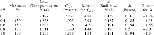
Details of maximum Reynolds number simulated for each
 $AR$
value, comparison of drag coefficients and Strouhal number with the literature.

2 Numerical details and validation
The governing equations of fluid flow and heat transfer around an arbitrarily shaped body in vector form are:
 $$\begin{eqnarray}\displaystyle & \displaystyle \unicode[STIX]{x1D735}\boldsymbol{\cdot }\boldsymbol{u}=0, & \displaystyle\end{eqnarray}$$
 $$\begin{eqnarray}\displaystyle & \displaystyle \frac{\unicode[STIX]{x2202}\boldsymbol{u}}{\unicode[STIX]{x2202}\unicode[STIX]{x1D70F}}+(\boldsymbol{u}\boldsymbol{\cdot }\unicode[STIX]{x1D735})\boldsymbol{u}=-\unicode[STIX]{x1D735}p+\frac{1}{Re}\unicode[STIX]{x1D6FB}^{2}\boldsymbol{u}+\boldsymbol{f}, & \displaystyle\end{eqnarray}$$
 $$\begin{eqnarray}\displaystyle & \displaystyle \frac{\unicode[STIX]{x2202}\boldsymbol{T}^{\,\ast }}{\unicode[STIX]{x2202}\unicode[STIX]{x1D70F}}+(\boldsymbol{u}\boldsymbol{\cdot }\unicode[STIX]{x1D735})\boldsymbol{T}^{\,\ast }=\frac{1}{RePr}\unicode[STIX]{x1D6FB}^{2}\boldsymbol{T}^{\,\ast }+\boldsymbol{q}, & \displaystyle\end{eqnarray}$$
where,
 $\boldsymbol{u},p,\unicode[STIX]{x1D70F}$
and
 $\boldsymbol{T}^{\,\ast }$
are the non-dimensional velocity, pressure, time and temperature respectively, while
 $Re$
and
 $Pr$
represent Reynolds and Prandtl numbers respectively. The Reynolds number (
 $Re$
) is given as,
 $Re=\unicode[STIX]{x1D70C}u_{\infty }2a/\unicode[STIX]{x1D707}$
, where,
 $\unicode[STIX]{x1D707}$
– viscosity of fluid. Hydraulic diameter (
 $D$
) is taken as the characteristic length to normalise the downstream distance behind the cylinder. The immersed boundary method (IBM) is used to solve the governing equations numerically. In (2.2) and (2.3), the additional terms represented by
 $\boldsymbol{f}$
and
 $\boldsymbol{q}$
are associated with the IBM which are the forcing terms for velocity and temperature fields respectively. These forcing terms are used to model the solid body and to apply velocity and thermal boundary conditions effectively. The convective and diffusive terms are discretized by the second-order central differencing scheme. Temporal discretization is done by the first-order Euler integration method. Detailed implementation of the algorithm and its preliminary validations including the grid independence study and the Lagrangian points independence study can be found in the references Raman, Prakash & Vengadesan (Reference Raman, Prakash and Vengadesan2013), Paul (Reference Paul2013), Paul et al. (Reference Paul, Arul Prakash and Vengadesan2013, Reference Paul, Arul Prakash and Vengadesan2014a
,Reference Paul, Arul Prakash and Vengadesan
b
).
The size of the computational domain is
 $-10D\leqslant x\leqslant 100D$
,
 $-10D\leqslant y\leqslant 10D$
. Uniform streamwise velocity and temperature profiles are imposed at the inlet, while fully developed flow conditions of velocity and temperature are applied at the outlet. The top and bottom sides of the computational domain are considered as free-slip walls in terms of both velocity and temperature. No-slip boundary conditions are imposed at the wall for velocity, while a uniform heat flux is imposed on the cylinder for temperature and a zero normal pressure gradient is applied for wall pressure. The elliptic cylinder is discretized with 315 Lagrangian marker points. The Eulerian domain is discretized with a non-uniform grid of 1271 and 845 grid points along the
 $x$
and
 $y$
directions respectively. A uniformly spaced grid is embedded around the elliptic cylinder for the effective use of the forcing function and to resolve the shear layer properly. The size of the uniform grid sized computational domain is (
 $-1.0D\leqslant x\leqslant 1.0D$
,
 $-1.0D\leqslant y\leqslant 1.0D$
) with the mesh size of
 $\unicode[STIX]{x0394}x=\unicode[STIX]{x0394}y=0.003$
.
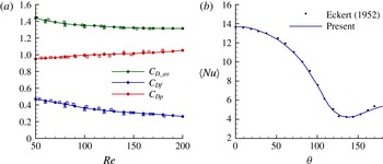
Validation of the solver pertaining to the viscous, pressure drag coefficients and the Nusselt number for the flow around circular cylinder is given in figure 1. From the figure, it is evident that current results are in good agreement with the literature. Concerning the validation for flow past the elliptic cylinder, the Strouhal number and drag coefficients for the highest
 $Re$
considered for each of the
 $AR$
values are compared with the literature (table 1). The present values are found to be in close agreement with the previous results for
 $St$
with an error of
 $\pm 2\,\%$
which is a reasonable validation. However, the drag coefficient is found to show some discrepancy which could be attributed to two factors. One is that the present results are obtained using a 5 % blockage computation domain while the paper of Thompson et al. (Reference Thompson, Radi, Rao, Sheridan and Hourigan2014) has a much lower blockage of 1 %. Secondly, we are comparing against the extrapolated values of
 $C_{D\_av}$
as Thompson et al. (Reference Thompson, Radi, Rao, Sheridan and Hourigan2014) do not have values for the
 $AR$
cases considered in this study.
(a) Comparison of viscous (
 $C_{Df}$
), pressure (
 $C_{Dp}$
) and total
 $(C_{D\_av})$
drag coefficients with literature (solid lines with symbol – present results, open triangle – Tritton (Reference Tritton1959), open squares – Henderson (Reference Henderson1995)). (b) Comparison of time-averaged Nusselt number with the results of Eckert (Reference Eckert1952) at
 $Re=180$
.

3 Results and discussion
3.1 Classification of flow regimes
The wakes are classified as: (i) regular von Kármán vortex shedding regime (R
 $v$
KVSR), (ii) broken von Kármán vortex shedding regime (B
 $v$
KVSR) and (iii) secondary von Kármán vortex shedding regime (S
 $v$
KVSR). The following subsections provide details of these wake types in terms of their flow and thermal properties in the order of: (i) vorticity pattern, (ii) evolution of wavelength of the vortex street in the wake, (iii) evolution of shape of the vortex street in the wake, (iv) streamlines pattern, (v) isotherm pattern, (vi) evolution of the mean temperature along the centreline with the mechanism of heat transport in the wake, (vii) Nusselt number profile with its heat transfer mechanism from the cylinder, (viii) temporal variation of instability and its Hopf bifurcation analysis, (ix) spatio-temporal diagram of instabilities and (x) shedding frequencies in the near and far wakes. Out of these properties, (ii) and (iii) require further explanation on how they are obtained. The wavelength of the vortex street is computed using the
 $\unicode[STIX]{x1D734}/\unicode[STIX]{x1D734}_{N}$
curve, where
 $\unicode[STIX]{x1D734}$
is the transversely integrated vorticity normalised by
 $\unicode[STIX]{x1D734}_{N}$
which is the average of the maximum absolute value of
 $\unicode[STIX]{x1D734}$
at all the
 $x/D$
locations. Subsequent maxima/minima in the
 $\unicode[STIX]{x1D734}/\unicode[STIX]{x1D734}_{N}$
curve give the wavelength of the vortex street. In order to discern the spatial evolution of shape of the vortex street, we form the following hypothesis. As vorticity is a passive object, it cannot cause changes to the flow field, rather it is the flow that acts on it. When looking at the transport equation of vorticity for a 2-D flow, it is evident that the vortex stretching term is absent, and the vortex can not be rotated or stretched by the strain-field. For two dimensions, the vorticity equation shows that the transport by flow is balanced by diffusion due to viscosity. Since diffusion is a homogeneous process, it is not expected to change the shape of a vortex. We are now left with the only remaining term, the transport by flow. Therefore, it is believed that the spatial evolution of shape of the vortex street is something to do with the flow, at least in a 2-D flow field. Based on this hypothesis, we compute the local flow behaviour and correlate it to the shape of the vortex street. As per the
 $\unicode[STIX]{x1D706}_{2}$
criterion (Jeong & Hussain Reference Jeong and Hussain1995), the flow has both shearing and swirling regions. We use the
 $\unicode[STIX]{x1D706}_{2}$
criterion to identify shearing and swirling flow regions and correlate them with vorticity through the
 $\unicode[STIX]{x1D734}_{shear}/\unicode[STIX]{x1D734}_{swirl}$
curve, where
 $\unicode[STIX]{x1D734}_{shear}$
is the transversely integrated enstrophy at all the points where
 $\unicode[STIX]{x1D740}_{2}>0$
and
 $\unicode[STIX]{x1D734}_{swirl}$
is the corresponding result for
 $\unicode[STIX]{x1D740}_{2}<0$
. Cumulative averaging is carried out on
 $\unicode[STIX]{x1D734}_{shear}$
and
 $\unicode[STIX]{x1D734}_{swirl}$
along the streamwise direction before taking the ratio between them. Here, the action of shear is to change the shape of the fluid element, and thus the vortex street, while the action of swirl is to increase the rotation of a vortex.
3.1.1 Regular von Kármán vortex shedding regime (R
 $v$
KVSR)

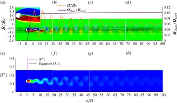
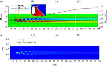
Vorticity contour of a typical R
 $v$
KVSR is shown in figure 2(a–d) for the case of
 $AR=1.0$
and
 $Re=50$
. The formation region exists close to the cylinder (from the lee of the cylinder to
 $x/D\approx 4$
) where the shear layers emanating from the top and bottom of the cylinder interact with each other. Adjacent to this region, the von Kármán region, which gains its name due to the presence of von Kármán vortex street, is observed. The vertical distance between the vortices is denoted by ‘
 $h$
’, while the horizontal distance between the similar sign vortices is marked by ‘
 $a$
’. The vortices do not seem to be changing their shape in the von Kármán region as perceived from figure 2(a–d) which provides a weak evidence that the von Kármán vortex street is non-dispersive in nature.
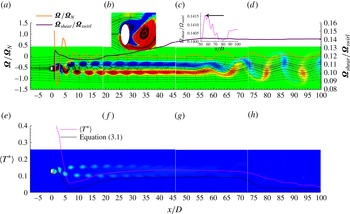
(a–d) Vorticity contour, (e–h) isotherms. Streamlines are superimposed over vorticity contours in (a–d) along with profiles of
 $\unicode[STIX]{x1D734}/\unicode[STIX]{x1D734}_{N}$
and
 $\unicode[STIX]{x1D734}_{shear}/\unicode[STIX]{x1D734}_{swirl}$
. Mean temperature evolution along the centreline is given in (e–h). Contour levels for vorticity, and temperature are:
 $-0.5$
(0.035) 0.5 and 0.011 (0.05) 0.44 respectively.

The wavelength of the vortex street is computed to be
 $8.1D$
from the
 $\unicode[STIX]{x1D734}/\unicode[STIX]{x1D734}_{N}$
curve (figure 2
a–d) for
 $AR=1.0$
and
 $Re=50$
which is in good agreement with the literature (Karasudani & Funakoshi Reference Karasudani and Funakoshi1994). This wavelength does not change or decreases only slightly in the downstream which is an inherent characteristic of the von Kármán vortex street. Decrease in amplitude of the
 $\unicode[STIX]{x1D734}/\unicode[STIX]{x1D734}_{N}$
curve shows that the energy of the vortex street is dissipated in the downstream due to diffusion. Our results re-ascertain the fact that the von Kármán vortex streets are non-dispersive travelling waves whose amplitudes decrease due to diffusion in the downstream direction (Karniadakis & Triantafyllou Reference Karniadakis and Triantafyllou1989). Although the nature of the vortex street is reported in the literature, the reason as to why they exhibit such a characteristic is not available.
Profile of
 $\unicode[STIX]{x1D734}_{shear}/\unicode[STIX]{x1D734}_{swirl}$
helps us to understand why the von Kármán vortex streets are non-dispersive. A steep positive slope of the
 $\unicode[STIX]{x1D734}_{shear}/\unicode[STIX]{x1D734}_{swirl}$
curve in the formation region indicates the action of shear domination. This means that the vorticity buildup occurs due to shear in the formation region close to the cylinder. As the flow is predominately in the
 $x$
-direction, this shear buildup causes the shear layers to stretch and orient along the streamwise direction. Around
 $x/D\approx 4$
, the slope of
 $\unicode[STIX]{x1D734}_{shear}/\unicode[STIX]{x1D734}_{swirl}$
turns to negative which shows the onset of swirl domination. This is also the location where the shear layers start to interact. It can be interpreted, therefore, that the onset of swirl domination causes the individual shearing layers (which are attached to the cylinder) to rotate, and to interact with each other. It is interesting to note that in the von Kármán region where the vortices are convected by the flow while diffusing vorticity, the curve remains a constant which is a sign that neither shear nor swirl dominates the individual vortex. This means that the vortices get convected downstream with the shape and swirl strength imposed on them by the flow at the end of the formation region. Therefore, the constant value of
 $\unicode[STIX]{x1D734}_{shear}/\unicode[STIX]{x1D734}_{swirl}$
might explain why von Kármán vortex streets are non-dispersive. Since each vortex has some swirling strength, due to the mean flow they have the tendency to move away from the centreline as they get convected. This could explain why increase in
 $h/a$
value was observed only due to increase in ‘
 $h$
’ in the previous studies (Hooker Reference Hooker1936).
Instantaneous streamline patterns of the R
 $v$
KVSR, as depicted in figure 2(a–d) show that the flow gets separated from the surface of the cylinder at two different separation points (inset figure in figure 2
a). However, a near-wall instantaneous recirculation region (NWIRcR) forms around only one separation point (it is seen in the bottom part of the cylinder in the inset figure 2
a). Standard streamlines properties such as the centre, saddle and alleyway can also be seen clearly in the inset figure. During a shedding cycle, the alleyways draw fluid from the bottom to top part of the cylinder, and the size of NWIRcR increases until it gets detached completely from the cylinder. This detachment gives rise to the formation of NWIRcR at the other separation point, and the same process continues in the reverse direction for the next half of a shedding cycle.
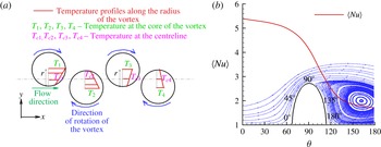
(a) Simplified schematic heat transport model for the R
 $v$
KVSR. (b) A typical
 $\langle Nu\rangle$
profile of R
 $v$
KVSR where the mean streamlines are depicted in the background.

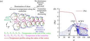
The isotherms pattern depicted in figure 2(e–h) are analogous to the vorticity patterns. The mean temperature profile along the centreline superimposed on figure 2(e–h) shows that the temperature is maximum at the wall, and it decreases monotonically to the value of the inlet temperature downstream. This variation is on the expected lines as the temperature, being a passive scalar, will only be convected downstream without causing any change to the flow characteristics. A simple heat transport model as depicted in figure 3(a) is constructed to explain the variation of mean temperature. Here, the von Kármán region is represented by repeating positive and negative vortices. Due to its rotational motion, the temperature inside the vortex is maximum at the centre, and it decreases to the free-stream temperature along the radius of a vortex. Due to the non-dispersive behaviour, these vortices get convected downstream without deteriorating in shape while diffusing energy. Therefore, at any vortex, the temperature at the centreline is less than its core temperature besides being below the centreline temperature of the previous vortex core. This explanation can be seen pictorially in figure 3(a) which shows that our model predicts qualitatively the same variation of temperature obtained by the simulation. We develop a semi-analytical expression for the variation of mean temperature along the centreline based on the aforementioned vortex dynamics. This expression is valid for all regions except the formation region. Initially, the vortex cores of individual vortices are assumed to be on the centreline, and the distribution of vortex core temperature downstream is computed by solving a 1-D heat equation with inhomogeneous boundary conditions. At the start of the von Kármán region,
 $T^{\,\ast }$
is obtained using the imposed heat flux (i.e.
 $T_{x/D=x/D_{vk}}^{\,\ast }=qD/k$
), and at the far downstream, the temperature is assumed to decay to 101 % of the free-stream value (i.e.
 $T_{x/D=100}^{\,\ast }=101\,\%\times T_{\infty }^{\,\ast }$
). Solution for this kind of equation can be found in any advanced mathematics text book and is therefore not repeated here. The vortex cores are then forced to move away from the centreline due to shear and swirl, and their movements are computed from the
 $\unicode[STIX]{x1D734}_{shear}/\unicode[STIX]{x1D734}_{swirl}$
curve. The final equation for mean temperature is:
 $$\begin{eqnarray}\langle T^{\,\ast }\rangle =\left\{\begin{array}{@{}ll@{}}\displaystyle {\displaystyle \frac{1}{\unicode[STIX]{x1D70F}_{2}-\unicode[STIX]{x1D70F}_{1}}}\int _{\unicode[STIX]{x1D70F}_{1}}^{\unicode[STIX]{x1D70F}_{2}}T^{\,\ast }(x,y_{i}(\unicode[STIX]{x1D70F}),\unicode[STIX]{x1D70F})\text{d}\unicode[STIX]{x1D70F},\quad & \text{if }y\leqslant R\\ \displaystyle {\displaystyle \frac{1}{\unicode[STIX]{x1D70F}_{2}-\unicode[STIX]{x1D70F}_{1}}}\int _{\unicode[STIX]{x1D70F}_{1}}^{\unicode[STIX]{x1D70F}_{2}}{T_{\infty }}^{\,\ast }\,\text{d}\unicode[STIX]{x1D70F},\quad & \text{otherwise},\end{array}\right.\end{eqnarray}$$
where,
 $R$
is the radius of the vortex which is equivalent to the radius of the cylinder and
 $T^{\,\ast }(x,y_{i}(\unicode[STIX]{x1D70F}),\unicode[STIX]{x1D70F})$
is given as:
 $$\begin{eqnarray}T^{\,\ast }(x,y_{i}(\unicode[STIX]{x1D70F}),\unicode[STIX]{x1D70F})={T_{1}}^{\,\ast }(x,\unicode[STIX]{x1D70F})\left[{\displaystyle \frac{R-y_{i}(\unicode[STIX]{x1D70F})}{R}}\right]+T_{\infty }\left[{\displaystyle \frac{y_{i}(\unicode[STIX]{x1D70F})}{R}}\right],\end{eqnarray}$$
where
 $T_{1}^{\,\ast }(x,\unicode[STIX]{x1D70F})$
is the solution of the inhomogeneous heat equation given in terms of steady and unsteady solution as:
 $$\begin{eqnarray}T_{1}^{\,\ast }(x,\unicode[STIX]{x1D70F})=T_{1}(x)+T_{2}(x,\unicode[STIX]{x1D70F}),\end{eqnarray}$$
where,
 $$\begin{eqnarray}T_{1}(x)=\left[\frac{T_{\infty }^{\,\ast }-\frac{qD}{k}}{L_{x}}\right]x+\frac{qD}{k},\end{eqnarray}$$
 $$\begin{eqnarray}T_{2}(x,\unicode[STIX]{x1D70F})=\frac{2}{\unicode[STIX]{x03C0}}\left[T_{\infty }-T(x)\right]\mathop{\sum }_{m=1}^{\infty }\frac{2}{2m-1}\text{e}^{-[((2m-1)\times Pr\times \unicode[STIX]{x03C0})/L_{x}]^{2}\unicode[STIX]{x1D70F}}\sin (2m-1)\frac{\unicode[STIX]{x03C0}}{L_{x}}x\end{eqnarray}$$
and
 $y_{i}$
(where ’
 $i$
’ is the index of the vortex) is the location of vortex cores obtained from the
 $\unicode[STIX]{x1D734}_{shear}/\unicode[STIX]{x1D734}_{swirl}$
curve, and is given as:
 $$\begin{eqnarray}y_{i}(\unicode[STIX]{x1D70F})=y_{i}(\unicode[STIX]{x1D70F}-\unicode[STIX]{x0394}\unicode[STIX]{x1D70F})+Y_{i},\end{eqnarray}$$
 $$\begin{eqnarray}Y_{i}={\displaystyle \frac{(-1)^{i+1}}{\sqrt{Re}}}{\displaystyle \frac{{\displaystyle \frac{\unicode[STIX]{x2202}\left({\displaystyle \frac{\unicode[STIX]{x1D734}_{shear}}{\unicode[STIX]{x1D734}_{swirl}}}\right)}{\unicode[STIX]{x2202}x}}}{\left|{\displaystyle \frac{\unicode[STIX]{x2202}\left({\displaystyle \frac{\unicode[STIX]{x1D734}_{shear}}{\unicode[STIX]{x1D734}_{swirl}}}\right)}{\unicode[STIX]{x2202}x}}\right|}}.\end{eqnarray}$$
The initial condition for
 $y_{i}(0)$
is assumed to be zero. This expression is semi-analytical due to the fact that the computation of
 $Y_{i}$
depends on the DNS data. The variation of
 $Y_{i}$
is very difficult to model as it depends on various factors including the blockage ratio. The comparison of this semi-analytical model with simulation shows satisfactory result for the R
 $v$
KVSR, as shown in figure 2(e–h).
Having discussed the heat transport in the wake, we focus now on heat transfer from the cylinder. Figure 3(b) shows the variation of the time-averaged Nusselt number (
 $\langle Nu\rangle$
) along the circumference of the cylinder from
 $0^{\circ }$
to
 $180^{\circ }$
, where
 $0^{\circ }$
is the front stagnation point,
 $180^{\circ }$
is the rear stagnation point and the variation is considered clockwise from
 $0^{\circ }$
to
 $180^{\circ }$
. The maximum heat transfer is at the front stagnation point and the heat transfer rate decreases along the circumference of the cylinder. In order to explain this
 $\langle Nu\rangle$
variation, time-averaged streamlines for the R
 $v$
KVSR are shown in the background of figure 3(b). The cold fluid from the inlet impinges first on the front stagnation point, causing the highest heat transfer at that point. Due to this impingement, it is now a warm fluid, with temperature higher than the inlet temperature, that passes over the rest of the surface causing less heat transfer than that of the front stagnation point. Around
 $100^{\circ }$
, the flow gets separated from the cylinder forming a clockwise vortex which curls through
 $110^{\circ }$
–
 $180^{\circ }$
. This clockwise vortex transports even more hot fluid towards the cylinder, which in turn decreases
 $\langle Nu\rangle$
rapidly. This trend is seen in the
 $\langle Nu\rangle$
variation in the same figure.
(a) Profiles of absolute amplitude of instabilities at different downstream locations, (b) profiles of
 $(\text{d}(\ln (|A|))/\text{d}t)$
against
 $|A|^{2}$
at different downstream locations.

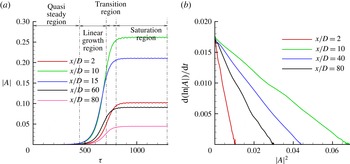
Figure 4(a) shows the variation of absolute magnitude of disturbances in time. This curve consists of four distinct regions namely, (i) quasi-steady, (ii) linear growth, (iii) transition and (iv) saturation regions. From
 $\unicode[STIX]{x1D70F}=0$
to a certain time, the flow proceeds towards a quasi-steady state where the maximum unsteadiness is very low. After the quasi-steady state, the disturbances grow linearly till the vortex shedding starts. The region where the shedding stabilises is identified by a slow, yet positive, slope of the
 $|A|$
–
 $\unicode[STIX]{x1D70F}$
curve, and it is called the transition region. After this, the disturbances reach a saturated state and the corresponding region is called the saturation region. The negative slope in the
 $(\text{d}(\ln (|A|))/\text{d}t)-|A|^{2}$
, curve as depicted in figure 4(b), indicates that the transition of R
 $v$
KVSR occurs through a supercritical Hopf bifurcation. The value of the amplification rate (
 $\unicode[STIX]{x1D6FE}$
) is calculated to be 0.01745, which matches well with the values obtained by Paul et al. (Reference Paul, Arul Prakash and Vengadesan2014b
). Also, the value of
 $\unicode[STIX]{x1D6FE}$
is global, which means its value does not change in the computational domain.
Spatio-temporal diagram of instabilities along the centreline: (a) R
 $v$
KVSR, (b) B
 $v$
KVSR, (c) S
 $v$
KVSR. (The contour levels of these figures are: 0 (0.05) 1.)

The spatio-temporal diagram of disturbances along the centreline for the R
 $v$
KVSR is shown in figure 5(a). The point
 $x/D=0$
in the figure is the location of rear stagnation point of the cylinder. For the R
 $v$
KVSR, a fixed time-dependent unstable wave packet of higher magnitude is observed downstream of the cylinder, and the magnitude of instability decreases in the downstream direction. The magnitude of the disturbance becomes almost zero near the outlet. This is because of the viscous diffusion due to higher viscosity which damps instability. At far downstream distances, the instabilities become time independent.
(a) Fast Fourier transform (FFT) analysis of velocity signals taken at different downstream locations, (b) FFT analysis for different regions at
 $x/D=40$
.

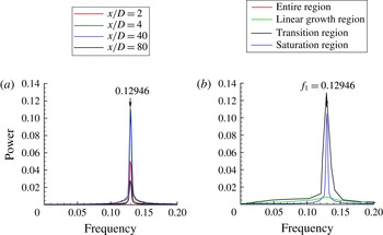
Fast Fourier transform (FFT) of velocity signals are performed in order to compute the frequency of vortex shedding. FFT analysis, as shown in figure 6(a), indicates that all the energy is concentrated at the fundamental frequency (
 $f_{1}=0.12946$
). As the flow has different regions, as shown in figure 4(a), we decompose the velocity signal to different subsignals corresponding to different regions in order to find the origin of the primary shedding frequency. FFT is then performed on these subsignals and the result is shown in figure 6(b) for
 $x/D=40$
. It can be seen from this figure that the primary frequency of vortex shedding arises from both transition and saturation regions.
3.1.2 Broken von Kármán vortex shedding regime (B
$v$
KVSR)

In order to discuss the typical characteristics of B
 $v$
KVSR, the case of
 $AR=0.4$
and
 $Re=100$
is considered. The vorticity contour has formation and von Kármán regions as shown in figure 7(a–d). At the end of the von Kármán region, the vortices become dispersive in nature as they get elongated both laterally and longitudinally. ‘Anisotropic extension’ is the term used in the literature to denote this process (Karasudani, Funakoshi & Oikawa Reference Karasudani, Funakoshi and Oikawa1989) through which the von Kármán vortex street loses its characteristics and becomes dispersive in nature. This anisotropic extension of vortices leads the primary vortex street to evolve into two rows of vortex chains where each row contains vortices of similar sign. Therefore, this region is called the parallel vortex region which is observed approximately for
 $x/D>2$
in the figure 7(a–d).
Caption is same as of figure 2.

Contours of instantaneous streamlines for the B
 $v$
KVSR, as shown in figure 7(a), reveal an interesting behaviour. The flow gets separated from the surface at two separation points located at the top and bottom parts of the cylinder, and the NWIRcR appears around both the points, which is entirely different from a single NWIRcR behaviour observed for the R
 $v$
KVSR. We call this dual near-wall instantaneous recirculation region (dual-NWIRcR) behaviour. During the first half of the B
 $v$
KVSR shedding cycle, one of these NWIRcR grows in size due to continuous pulling of fluid by the alleyways. At the end of a half stage of the cycle, the growth of this NWIRcR reaches a maximum as it merges with the other NWIRcR, and they move away from the cylinder as a single blob of closed streamlines. This process repeats itself for the next half of the shedding cycle. In the parallel vortex region, the streamlines appear near straight lines.
Variation of length of von Kármán region with respect to
 $Re$
for the case of the B
 $v$
KVSR at
 $AR=0.4$
.

The important thing to notice in the streamlines pattern of the B
 $v$
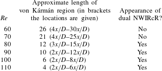
KVSR is the appearance of dual NWIRcR. After a detailed analysis of all the cases considered in this study, it is found that the appearance of a dual NWIRcR is dependent on the length of the von Kármán region. For example, the authors have computed the length of the von Kármán region besides checking for the NWIRcR for the cases which are classified under B
 $v$
KVSR. The results are presented in table 2 for
 $AR=0.4$
. From the table, it can be clearly seen that not all vortex shedding regions that belong to the B
 $v$
KVSR exhibit the dual-NWIRcR behaviour, but it strongly depends on length of the von Kármán region. For higher lengths, there is no appearance of the dual NWIRcR. When the length of the von Kármán region becomes short, the dual NWIRcR appears. After this analysis, we propose as a rule of thumb that in order for the dual NWIRcR to appear, the length of the von Kármán region should be less than
 $15x/D$
. This solves the puzzle and explains why previous studies on circular cylinder at low Reynolds numbers did not predict this phenomenon even though flow past circular cylinder above
 $Re=150$
falls under the category of B
 $v$
KVSR. As the length of the von Kármán region is of the order of
 $30x/D$
for flow around a circular cylinder in the laminar region (i.e. for
 $Re\leqslant 200$
), the dual-NWIRcR behaviour cannot be observed there.
The
 $\unicode[STIX]{x1D734}/\unicode[STIX]{x1D734}_{N}$
curve for the B
 $v$
KVSR, as depicted in figure 7(a–d), shows oscillations in the formation and the von Kármán regions which measure the wavelength of the primary vortex street. These oscillations die out completely in the parallel vortex region which shows suppression of the primary vortex street. Unlike the R
 $v$
KVSR, where vorticity buildup due to shear happened for a relatively longer distance, the steep slope in the
 $\unicode[STIX]{x1D734}_{shear}/\unicode[STIX]{x1D734}_{swirl}$
curve for the B
 $v$
KVSR is very short, and then the slope changes to negative. The slope change in
 $\unicode[STIX]{x1D734}_{shear}/\unicode[STIX]{x1D734}_{swirl}$
for the B
 $v$
KVSR also happens instantly (this slope change was slow for the R
 $v$
KVSR), and the negative slope exists for a longer distance. This evidence shows that the shear layers from the cylinder are stretched along the streamwise direction only for a short distance (which also accounts for a very short formation region) and the flow exports a higher amount of swirl in order for the individual vortices to form. These higher swirlings give the individual vortices the tendency to move away from the centreline, which in turn increases the
 $h/a$
ratio. The value of
 $\unicode[STIX]{x1D734}_{shear}/\unicode[STIX]{x1D734}_{swirl}$
is not constant, as in the case of R
 $v$
KVSR, but increases along the von Kármán and the parallel-flow regions which indicates the continuous stretching of the individual vortices along the streamwise direction. As a result, the individual vortices of the von Kármán vortex street changes its shape and gets oriented along the streamwise direction. In summary, the genesis of the individual vortices is marked by higher swirl at the end of the formation region, and the vortices are then under the constant action of shear for the entire computational domain. Due to these, the usual von Kármán breaks down and becomes dispersive in nature.
The contour of isotherm for the case of B
 $v$
KVSR is also analogous to its vorticity contour (figure 7
e–h). The mean temperature profile in the von Kármán region of the B
 $v$
KVSR is qualitatively similar to that of the R
 $v$
KVSR where the temperature decreases monotonically from the wall. Therefore, the model discussed for the R
 $v$
KVSR can be used in these regions to study the transport of heat. It is very interesting to see from figure 7(e–h) that the temperature starts to increase from the point of vortex street breakdown to the end of the parallel vortex region. It is computed that a 35 % increase in temperature happens locally in these regions. This is a perplexing situation as it is intuitive that the magnitude of a passive scalar such as the temperature cannot increase suddenly without any source of heating. The authors have constructed an effective simple model to answer this question. The model is depicted in figure 8(a), and it is applicable for the parallel vortex region. The physical mechanism involved in this model is discussed as follows.
(a) Simplified schematic heat transport model for the B
 $v$
KVSR. (b) A typical
 $\langle Nu\rangle$
profile of B
 $v$
KVSR where the mean streamlines are depicted in the background.

At the beginning of the parallel vortex region, the horizontal distance between the same sign vortices (represented as
 $w_{1}$
in figure 8
a) and the vertical distances (represented as
 $h_{1}$
in figure 8
a) between the vortex pair (i.e. vortices of opposite signs) are larger because of the movement of vortices away from the centreline due to the fact that the flow exerts higher swirl on fluid element as discussed from the
 $\unicode[STIX]{x1D734}_{shear}/\unicode[STIX]{x1D734}_{swirl}$
curve. It is observed from the heat flux vector plots that the core temperatures of the individual vortices in each of these vortex pair are almost equal. For simplicity purpose, let us take these values as equal and at
 $T_{1}$
. Since the distance between vortices in a vortex pair is high for the first vortex, temperature varies for a longer distance. As a result, temperature at the centreline will be lower. As already discussed, shear starts dominating in the parallel vortex region. This causes individual vortices to shrink and come closer to each other as well as closer to the centreline. Therefore, for the second vortex pair, the temperature varies for a shorter distance because of its locality. Due to this, the temperature at the centreline will be higher than
 $T_{c1}$
even though
 $T_{2}\approx T_{1}$
. This process repeats and the vortices of the vortex pair continues to move closer to each other as long as the shear domination exists. At the end of the shear domination region, temperature along the centreline will read as
 $T_{c1}$
 ${<}$
 $T_{c2}$
 ${<}$
 $T_{c3}$
 ${<}$
 $T_{c4}$
which is also manifested in the temperature profile obtained through the simulation. From this, it is evident that our model predicts the similar temperature profile obtained in our simulation. Besides this, we are able to understand the mechanism of transport of heat when the shedding pattern is B
 $v$
KVSR. Our semi-analytical model is again applied for this wake type, and found to be producing similar trend of the mean temperature obtained from the simulation. The values obtained from (3.1) are slightly off mainly because of the difficulty in arriving at an accurate boundary condition for
 $T^{\,\ast }$
at the starting of the von Kármán region. This is because of the complexities involved with the dual NWIRcR due to which the temperature at the wall varies drastically. However, our model still succeeded in arriving at the trend of mean temperature which also validates the hypothesis used for constructing the heat transport model.
The mean streamlines of B
 $v$
KVSR with single NWIRcR is observed to be similar to that of the R
 $v$
KVSR. Therefore, the surface heat transfer mechanism discussed for R
 $v$
KVSR holds true for B
 $v$
KVSR cases with single NWIRcR. Distribution of
 $\langle Nu\rangle$
for the B
 $v$
KVSR with dual NWIRcR is shown in figure 8(b). The interesting thing to observe here is the secondary peak in the
 $\langle Nu\rangle$
which is marked as a red coloured arrow in figure 8(b). In order to discuss the source of this secondary peak, the time-averaged streamlines are given in the background image of figure 8(b). As analysed earlier, these patterns exhibit dual NWIRcR which manifest into two mean vortices for each of the NWIRcR when the flow is averaged in time as seen in figure 8(b). In the leeward surface, the flow gets separated from the cylinder. However, due to the dual-NWIRcR phenomenon, two counter-rotating vortices are present from
 $95^{\circ }$
to
 $180^{\circ }$
. The clockwise vortex which lies along
 $95^{\circ }$
–
 $128^{\circ }$
(marked as CWV in figure 8
b) takes hot fluid towards the cylinder and thus an equivalent decrease in
 $\langle Nu\rangle$
is observed. Close to the clockwise vortex, there exists a counter-clockwise vortex along the region of
 $125^{\circ }$
–
 $180^{\circ }$
which is marked as ACWV in figure 8(b). This anti-clockwise vortex takes cold fluid into the surface and thus increases the heat transfer. This is why the Nusselt number curve starts increasing after
 $125^{\circ }$
. Therefore, it is evident that the flow patterns with dual NWIRcR will have heat transfer increase in both the windward and leeward surfaces of the cylinder, and the physical mechanism responsible for such heat transfer enhancement is identified.
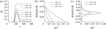
(a) Profiles of amplitude of disturbances at different downstream locations, (b,c) profiles of
 $(\text{d}(\ln (|A|))/\text{d}t)$
against
 $|A|^{2}$
at different downstream locations.

Temporal evolution of disturbances for the B
 $v$
KVSR is shown in figure 9(a). As observed in the R
 $v$
KVSR, here also four distinct regions can be seen in the profile. However, the main difference is spotted in the nonlinear transition region (for
 $200<\unicode[STIX]{x1D70F}<300$
) where the slope of
 $|A|$
–
 $\unicode[STIX]{x1D70F}$
becomes negative. This shows that the disturbances start decreasing or damping out before the vortex shedding stabilises. In other words, transition to saturation state in the B
 $v$
KVSR occurs through a nonlinear transition which is characterised by a negative slope in
 $|A|$
–
 $\unicode[STIX]{x1D70F}$
curve. The saturation amplitude continues to decrease along the downstream, in fact this value reaches zero for
 $x/D=50$
. Therefore, the flow in the parallel vortex region can be considered as a nominally steady flow.
The nonlinear transition characteristics of the B
 $v$
KVSR system as depicted in figure 9(b,c) show another intriguing behaviour. In the regions where single frequency is captured, the
 $(\text{d}(\ln (|A|))/\text{d}t)-|A|^{2}$
curves are perfectly straight lines with a negative slope near the
 $y$
-axis. Therefore, the transition type of B
 $v$
KVSR in the von Kármán region is the supercritical Hopf bifurcation. However, whenever multiple frequencies are observed, the transition characteristic curve no longer remains a straight line (figure 9
c). This is possible either because of the occurrence of double Hopf bifurcation at the same time instant, or the order of the Landau equation considered in this study is no longer sufficient for the B
 $v$
KVSR, and higher-order terms should be included in the Landau equation. This question is left open here as this requires further studies on this issue. It should also be noted that the Landau constants are not global for the B
 $v$
KVSR.
The spatio-temporal variation of instabilities at the centreline are shown in figure 5(b). Near the rear stagnation point, a higher magnitude of fixed instability wave packet is present in the spatial variation of instability whose trend is observed to be highly sensitive to time. For example, at some lower intermediate time, say
 $\unicode[STIX]{x1D70F}=210$
, the magnitude of the instabilities continues to decrease downstream. This indicates that at that time instant, only von Kármán vortex shedding is present throughout the downstream portion. At some higher intermediate time, for example at
 $\unicode[STIX]{x1D70F}=350$
, instabilities formed behind the cylinder decay rapidly and then it gains in magnitude and propagates again closer to the outlet. This can be interpreted as formation of primary shedding behind the cylinder, and then a parallel vortex region followed by a secondary shedding. At a higher time of the simulation, say at
 $\unicode[STIX]{x1D70F}=600$
, the instabilities created behind the cylinder decay rapidly to zero within a fewer downstream distance from the cylinder, and never regain their magnitudes downstream until the outlet. This behaviour shows that the secondary vortex shedding observed at some higher intermediate time has somehow vanished at larger times. This particular observation leads to a statement that the secondary shedding may be a time-dependent phenomenon even though we do not have a definite conclusion at this moment.
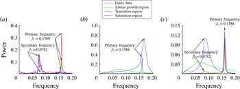
(a) FFT analysis of velocity signals taken at different downstream locations. (b) Signal decomposition method applied for a signal at
 $x/D=8$
. (c) Signal decomposition method applied for a signal at
 $x/D=32$
.

FFT performed on the near-wake velocity signals indicate that the energy is concentrated in one particular frequency which is the frequency of the von Kármán shedding (figure 10
a). Secondary frequencies start to appear around
 $x/D=28$
although they are not dominant frequencies at that location. Power of this secondary frequency grows downstream and becomes a dominant frequency around
 $x/D=50$
. After
 $x/D=50$
, the secondary frequency increases in power. Though some tertiary frequencies appear after
 $x/D=50$
, they are not definite in value (i.e. they keep changing their values from one location to another) besides, they are not dominant frequencies.
As mentioned earlier, Johnson et al. (Reference Johnson, Thompson and Hourigan2004) were the first to detect low-frequency unsteadiness in their numerical simulation of flow past an elliptic cylinder of
 $AR=0.25$
at
 $Re=100$
. Saha (Reference Saha2007) observed low-frequency unsteadiness in the wakes of flat plates. In this study, we try to explain this phenomenon using the signal decomposition method that we introduced earlier. When applying this method for a velocity signal taken at the von Kármán region, the result as presented in figure 10(b) shows that the primary frequency is coming from both the transition as well the saturation regions. When we probe the location where the primary and secondary frequencies are present yet the primary frequency is still the dominant frequency, the result shows that the primary frequency is arising from the saturation region while the nonlinear transition region, which has a negative
 $|A|$
–
 $\unicode[STIX]{x1D70F}$
slope, is responsible for the secondary frequency (figure 10
c). Analysing the spatial location where only the secondary frequency is present shows (figure not shown) that the secondary frequency is due to the transition region, and the saturation region does not show any meaning as velocities are zero in these locations. In summary, this study, for the first time, reports that the low secondary frequency in the far wake is coming from the transition region which should have a negative
 $|A|$
–
 $\unicode[STIX]{x1D70F}$
slope, and the saturation region is responsible only for the primary shedding frequency.
3.1.3 Secondary von Kármán vortex shedding regime (S
$v$
KVSR)

A vorticity contour of a typical S
 $v$
KVSR is shown in figure 11(a–d) for the case of
 $AR=0.4$
at
 $Re=130$
. The parallel vortex region observed in the B
 $v$
KVSR becomes unstable for higher
 $Re$
or lower
 $AR$
values, and starts to undulate in the S
 $v$
KVSR. Therefore, secondary vortex shedding (SVS) region appears adjacent to the parallel vortex region. A secondary vortex street appears in the SVS region which looks like the von Kármán vortex street.
Caption is same as of figure 2.

Streamline patterns of the S
 $v$
KVSR also exhibit the dual-NWIRcR behaviour (see the inset in figure 11
b). Since the length of the von Kármán region in the S
 $v$
KVSR is very short (of the order of
 $2x/D$
), occurrence of the dual NWIRcR here becomes completely independent of any parameter, and they appear in all the cases that are classified under the S
 $v$
KVSR. Streamlines in the SVS region are oscillatory in nature, which shows that the flow is unsteady and secondary vortex shedding exists.
The curve of
 $\unicode[STIX]{x1D734}/\unicode[STIX]{x1D734}_{N}$
shows a sinusoidal character with decreasing amplitude downstream in the formation and von Kármán regions. This sinusoidal variation denotes the existence of the primary von Kármán vortex street whose wavelength is computed to be
 $4.1D$
. In the parallel vortex region, the
 $\unicode[STIX]{x1D734}/\unicode[STIX]{x1D734}_{N}$
curve becomes a straight line of zero value which is a sign of suppression of the primary vortex street. In the SVS region, the curve starts to exhibit a sinusoidal characteristic again, but this time with increasing wavelength along the downstream. This trend is the representation of the secondary vortex street whose wavelength is calculated to be
 $11.36D$
which is almost three times that of the primary vortex street. This wavelength continues to increase downstream. This evidence reveals that both small-scale structures (primary vortex street) as well as large-scale structures (secondary vortex street) are present in the S
 $v$
KVSR.
An initially positive then a negative slope in the
 $\unicode[STIX]{x1D734}_{shear}/\unicode[STIX]{x1D734}_{swirl}$
curve is a possible answer for a very short formation region. Vorticity buildup is mainly due to shear in the parallel vortex region as the
 $\unicode[STIX]{x1D734}_{shear}/\unicode[STIX]{x1D734}_{swirl}$
exhibits a steady increase in that region. This domination of shear at the start of the parallel-flow region makes the vortices stretch, as discussed earlier. Once the parallel vortex region ends, it is very interesting to observe in the inset of figure 11(b) that the slope of the
 $\unicode[STIX]{x1D734}_{shear}/\unicode[STIX]{x1D734}_{swirl}$
curve suddenly becomes negative. This change in slope denotes the change from shear to swirl at the entrance of the SVS region. This dominant swirling motion in the SVS region causes the row of similar sign vortices to interact with each other, and causes individual vortices of higher swirl to form. Moving downstream in the SVS region, it is found that the shear and swirl are not equal, but swirl continues to increasingly dominate. This trend reveals that once the secondary vortex street is formed, its individual vortices continue to grow in swirling strength rather than only being convected like the vortices of the primary von Kármán vortex street. This explains the physical mechanism of formation of the secondary vortex street and answers why they are higher in wavelength.
Isotherms and mean temperature profiles of the S
 $v$
KVSR are shown in figure 11(e–h). Temperature decreases in the von Kármán region while it increases in the initial part of the parallel vortex region. Therefore, in the von Kármán and SVS regions, the model discussed for the R
 $v$
KVSR will explain the mechanism of heat transport, while the model of the B
 $v$
KVSR will do the same for the parallel vortex region. Once again, our semi-analytical expression for mean temperature is found to produce the trend obtained using simulation. Primarily due to the dual NWIRcR, the mean temperature values are not exactly matching with the simulation values.
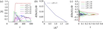
(a) Profiles of amplitude of disturbances at different downstream locations. (b,c) Profiles of
 $(\text{d}(\ln (|A|))/\text{d}t)$
against
 $|A|^{2}$
at different downstream locations.

The temporal variation of disturbances at various centreline locations are shown in figure 12(a) for the S
 $v$
KVSR. Only in the von Kármán region the disturbances grow linearly and transition to saturation state occurs with a positive slope in
 $|A|$
–
 $\unicode[STIX]{x1D70F}$
curve. In the parallel vortex and SVS regions, the disturbances grow linearly, and transition happens through a negative
 $|A|$
–
 $\unicode[STIX]{x1D70F}$
slope. The difference between the B
 $v$
KVSR and S
 $v$
KVSR regions comes in terms of the saturation region in the
 $|A|$
–
 $\unicode[STIX]{x1D70F}$
curve. While the disturbances eventually reach a saturated state with lower amplitude for the case of B
 $v$
KVSR, they never reach to the saturated state in the S
 $v$
KVSR. This trend is clearly visible in the curves plotted for
 $x/D=60$
and 80 in figure 12(a). The nonlinear transition characteristics curves in the parallel vortex and SVS regions show chaotic behaviour as depicted in figure 12(c). However, the transition of the von Kármán region occurs through a supercritical Hopf bifurcation as positive slope in
 $(\text{d}(\ln (|A|))/\text{d}t)$
–
 $|A|^{2}$
curve near the
 $y$
-axis is observed (figure 12
b).
The spatio-temporal variation of instabilities for the case of S
 $v$
KVSR draws more attention. The contour is almost similar to that of the B
 $v$
KVSR except the instabilities at the outlet do not die out. The crucial portion in the contour is the portion top of the arrow mark in figure 5(c). This region of interest contains instabilities of comparable magnitude which are nothing but the secondary vortex shedding. However, the size of this region keeps shrinking with time. If this contour follows the trend of the B
 $v$
KVSR (figure 5
b), this secondary shedding region will damp out at some point of time. However, it should be also be noted that the temporal variation of disturbances never reaches the saturation state in the S
 $v$
KVSR, and it is possible that these instabilities may never die out. Therefore, it can be stated that the secondary vortex streets are time-dependent phenomena. More studies are required to ascertain this result.
(a) FFT analysis of velocity signals taken at different downstream locations. (b) Signal decomposition method applied to a signal at
 $x/D=84$
.

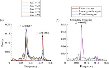
FFT of velocity signals are carried out and plotted in figure 13(a). A well-defined single frequency (the primary vortex shedding frequency) of value 0.1588 is observed for the formation and von Kármán regions. A secondary low frequency starts appearing at the initial part of the parallel vortex region (i.e.
 $x/D=12$
) but as a non-dominant frequency. This secondary frequency becomes dominant around
 $x/D=22$
with the primary frequency still apparently visible with lesser power. Around
 $x/D=58$
, the primary frequency vanishes completely and the secondary frequency becomes an absolute dominant frequency. After
 $x/D=58$
, the velocity spectrum shows only one dominant frequency with some noise. When applying the signal decomposition method in the locations where the flow does not reach the saturation state, it is observed that the transition state is fully responsible for the secondary frequency (see figure 13
b). Therefore, when the flow does not reach a saturation state, it will contain only the secondary frequency. Also, the value of the secondary frequency (0.0757) is not a multiple of the primary frequency. This evidence dismisses the possibility of secondary vortex street forming due to vortex pairing (Thompson et al.
Reference Thompson, Radi, Rao, Sheridan and Hourigan2014).
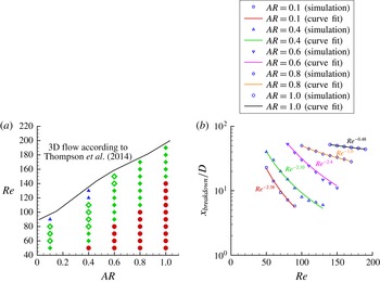
(a) Parameter space graph of all the identified flow patterns (circle – R
 $v$
KVSR, filled diamond – B
 $v$
KVSR without dual NWIRcR, open diamond – B
 $v$
KVSR with dual NWIRcR, triangle – S
 $v$
KVSR). (b) Curve fits for
 $x_{breakdown}/D$
.

We close this section by providing a parametric space graph of these three wake states. Such a graph was first constructed for flow past elliptic cylinders by Park et al. (Reference Park, Park and Hyun1989), and later by Johnson et al. (Reference Johnson, Thompson and Hourigan2001) and Johnson et al. (Reference Johnson, Thompson and Hourigan2004). Here, we provide an upgraded version of their graph which is depicted in figure 14(a). This graph not only gives information of the type of flow pattern but also helps us to study the effect of
 $AR$
,
 $Re$
on these flow regimes. It is observed from the figure that the tendency for the von Kármán vortex street to breakdown increases when the
 $AR$
of the elliptic cylinder decreases. There is no secondary shedding observed for flow around circular cylinder and elliptic cylinder of
 $AR=0.8$
within a computational domain of downstream distance of
 $100D$
. For the combination of smaller
 $AR$
values and higher
 $Re$
, a S
 $v$
KVSR type of flow pattern is observed. It is also understood from figure 14(a) that the instabilities in flow become stronger when
 $AR$
is decreased or
 $Re$
is increased.
3.2 Onset of the primary vortex street breakdown
In this section, the
 $x/D$
location at which the von Kármán vortex street breakdown occurs (
 $x_{breakdown}/D$
) is computed. Computing
 $x_{breakdown}/D$
is of importance as the mean temperature starts increasing from this very location. Two distinct approaches are utilised in order to calculate
 $x_{breakdown}/D$
. The first approach is based on flow visualisation method where vorticity contours are used to identify for the parallel vortex region. The point at which the vortex street breakdown occurs is identified by the appearance of side by side vortices. Secondly, we make use of the
 $\unicode[STIX]{x1D734}/\unicode[STIX]{x1D734}_{N}$
curve which gives the location of
 $x_{breakdown}$
when the differentiation of
 $\unicode[STIX]{x1D734}/\unicode[STIX]{x1D734}_{N}$
with
 $x$
becomes zero.
Curve fit performed over these data points helps us to study the dependence of
 $x_{breakdown}$
on
 $Re$
. For circular cylinder, the current study predicts a power-law relationship between
 $x_{breakdown}$
and
 $Re$
with the exponent value of
 $-0.48$
. Vorobieff, Georgiev & Ingber (Reference Vorobieff, Georgiev and Ingber2002) found a scaling of
 $Re^{-1/2}$
for the onset of second wake. For
 $AR=0.1$
, 0.4, 0.6 and 0.8 the scales are computed to be
 $Re^{-2.38}$
,
 $Re^{-2.1}$
,
 $Re^{-2.4}$
and
 $Re^{-1.0}$
respectively (figure 14
b).
4 Conclusions
An in-depth near- and far-wake analysis of flow past elliptic cylinders is carried out for diverse
 $Re$
and
 $AR$
values using the immersed boundary method based direct numerical simulations. Different flow patterns observed behind the elliptic cylinders are classified with the help of various postprocessing tools. Besides characterisation of flow regimes, this study also provided lucid explanations for the non-dispersive nature of the von Kármán vortex street, and the far-wake low-frequency unsteadiness. The mechanism of the secondary vortex shedding is predicted along with mechanism of the vortex street breakdown. Scaling laws for the primary vortex street breakdown are derived. Novel heat transport models are developed that solve the puzzle of abnormal temperature variation downstream to the elliptic cylinder.
Acknowledgements
The authors gratefully acknowledge the insightful and constructive comments of three anonymous reviewers, in particular of referee 2 which immensely helped to improve the quality of this paper substantially.