1 Introduction
The resonant oscillations of a water column in the gap formed between two closely spaced floating structures or the moonpools of drilling vessels have attracted extensive attention in recent decades due to their engineering significance. In addition to physical model tests, the methods of investigation mainly include two types of numerical model. One is based on potential flow theory, and the other is based on a viscous flow model using computational fluid dynamics (CFD); these types of models are referred to as the potential flow model and CFD model, respectively, hereafter. Although CFD models have recently shown reasonable success in solving gap resonance problems (Kristiansen & Faltinsen Reference Kristiansen and Faltinsen2008, Reference Kristiansen and Faltinsen2010; Lu et al. Reference Lu, Cheng, Teng and Zhao2010; Lu & Chen Reference Lu and Chen2012; Fredriksen, Kristiansen & Faltinsen Reference Fredriksen, Kristiansen and Faltinsen2015; Moradi, Zhou & Cheng Reference Moradi, Zhou and Cheng2015, Reference Moradi, Zhou and Cheng2016), they are computationally expensive for practical engineering applications. In contrast, potential flow models based on boundary/finite element methods in the frequency/time domain (e.g. Sun, Eatock Taylor & Taylor Reference Sun, Eatock Taylor and Taylor2010; Uzair & Koo Reference Uzair and Koo2012; Feng & Bai Reference Feng and Bai2015) and semi-analytical methods (Molin Reference Molin2001; McIver Reference McIver2005; Faltinsen, Rognebakke & Timokha Reference Faltinsen, Rognebakke and Timokha2007; Yeung & Seah Reference Yeung and Seah2007; Zhou, Wu & Zhang Reference Zhou, Wu and Zhang2013; McIver & Porter Reference McIver and Porter2016) are computationally efficient and widely used. However, the conventional potential flow models generally significantly over-predict the resonant response amplitudes due to the omission of the energy dissipation induced by the wall friction and flow separation. Efforts have been made to modify potential flow models by introducing an artificial viscous damping mechanism (or coefficient) while maintaining the computational efficiency (Molin et al. Reference Molin, Remy, Kimmoun and Stassen2002, Reference Molin, Remy, Camhi and Ledoux2009; Chen Reference Chen2004; Pauw, Huijsmans & Voogt Reference Pauw, Huijsmans and Voogt2007; Lu et al. Reference Lu, Teng, Cheng and Chen2011a ,Reference Lu, Teng, Sun and Chen b ; Liu & Li Reference Liu and Li2014). Modified potential flow models can predict resonant response amplitudes correctly with a predetermined damping coefficient, which is normally determined through trial-and-error tuning against experimental or CFD data. One concern about this type of modified potential flow model is whether the tuned damping coefficient remains valid for conditions that are beyond the parameter range of the experimental data or when extrapolated to prototype conditions.
Faltinsen & Timokha (Reference Faltinsen and Timokha2015) studied two-dimensional piston mode sloshing in a rectangular moonpool under forced heave motions. In their work, a pressure drop term representing the pressure discharge in the moonpool opening is directly introduced in the dynamic free-surface condition of a modified potential flow model inside the moonpool to account for the viscous damping involved in the fluid motion in/out of the moonpool. The pressure drop coefficient was determined through a known empirical formula for oscillatory flow through slotted screens (Faltinsen, Firoozkoohi & Timokha Reference Faltinsen, Firoozkoohi and Timokha2011). Significantly, the introduced damping mechanism is directly related to the underlying physics of the problem and no numerical tuning is required. The determination of the damping coefficient in the system relies on the known values for
 $b_{\ast }$
and the pressure drop coefficient
 $K(Sn,K_{c})$
(
 $Sn$
is the solidity ratio,
 $K_{c}$
is the Keulegan–Carpenter number), which are available for a moonpool entrance with sharp corners. The parameter
 $b_{\ast }$
was originally proposed by Molin (Reference Molin2001) to estimate the resonant frequency of the piston mode fluid oscillation in a moonpool and specifically represents the added mass of the oscillating fluid bulk. Faltinsen & Timokha (Reference Faltinsen and Timokha2015) assumed a pair of artificial impermeable vertical plates beneath a barge with a rectangular moonpool so that they could utilize the similarity between the piston-mode fluid motions in the moonpool and the oscillatory flow in a slot in a slatted screen. The parameter
 $b_{\ast }$
is used to denote half of the distance between the fictitious vertical plates, and the solidity ratio
 $Sn$
is defined as
 $Sn=(2b_{\ast }-1)/(2b_{\ast })$
. Because the determination method for
 $b_{\ast }$
is specifically designed for moonpool problems, it is uncertain whether the damping coefficient used in Faltinsen & Timokha (Reference Faltinsen and Timokha2015) is also applicable for gap resonance problems with a different geometry from the sharp-corner entrance and deep drafts. Despite this uncertainty, the method proposed by Faltinsen & Timokha (Reference Faltinsen and Timokha2015) is generally applicable for applications where the pressure drop coefficient is known.
The objective of the present study is to develop a viscous damping model that can be implemented in a potential flow model in the frequency domain by considering damping induced by both flow separation and wall friction. The remainder of the paper is organized as follows. The problem is stated in § 2, and a viscous damping model is introduced in § 3. The quantification method for the local and friction loss coefficients is reported in § 4. The implementation of the viscous damping model in a potential flow model is presented in § 5. Physical experiments are reported in § 6. Comparisons of the numerical results with experimental results are described in § 7. The method of estimating the frictional damping force and extensions of the presented methodology to general situations are discussed in § 8. Conclusions are finally drawn in § 9.
2 Statement of the problem
Sketch of the gap resonance between two fixed identical boxes with a curved gap entrance, where
 $\overline{h}$
is the water depth from the mean water level to the seabed,
 $\overline{B}$
is the breadth of the box,
 $L_{1}$
is the gap width,
 $\overline{d}$
is the draft of the floating boxes and
 $\overline{R}$
is the radius of the quarter circles used to form the gap entrance.

The physical problem considered in this study involves two identical, closely spaced fixed boxes subjected to incident waves from the left, as illustrated in figure 1. It is assumed that the dimension of the body in the direction perpendicular to the
 $\overline{x}$
–
 $\overline{z}$
plane is infinite. Thus, the problem can be simplified as a two-dimensional (2-D) problem. Of interest in this study is the piston-mode resonant response of the fluid trapped in the narrow gap and excited by a harmonic incident wave train. To facilitate the discussion presented in this study, the normalization method used by Faltinsen & Timokha (Reference Faltinsen and Timokha2015) is adopted. Specifically the length and time scales used in the normalization are, respectively, the gap width
 $L_{1}$
and the inverse of the angular frequency of the incident waves (
 $1/\unicode[STIX]{x1D70E}=T/2\unicode[STIX]{x03C0}$
, with
 $T$
the wave period). The following normalizations are used throughout the article unless otherwise specifically mentioned:
 $$\begin{eqnarray}\displaystyle \left.\begin{array}{@{}c@{}}\displaystyle x=\frac{\overline{x}}{L_{1}},\quad z=\frac{\overline{z}}{L_{1}},\quad t=\unicode[STIX]{x1D70E}\overline{t},\quad \unicode[STIX]{x1D6EC}=\frac{L_{1}}{g}\unicode[STIX]{x1D70E}^{2},\quad \unicode[STIX]{x1D713}(x,z,t)=\frac{\overline{\unicode[STIX]{x1D713}}(\overline{x},\overline{z},\overline{t})}{\unicode[STIX]{x1D70E}L_{1}^{2}},\\ \displaystyle h=\frac{\overline{h}}{L_{1}},\quad B=\frac{\overline{B}}{L_{1}},\quad d=\frac{\overline{d}}{L_{1}},\end{array}\right\}\qquad & & \displaystyle\end{eqnarray}$$
where variables marked by an overbar are dimensional variables,
 $\unicode[STIX]{x1D6EC}$
is the non-dimensional wave frequency,
 $\unicode[STIX]{x1D713}(x,z,t)$
is the dimensionless velocity potential,
 $g$
is the acceleration due to gravity,
 $L_{1}$
is the gap width,
 $\unicode[STIX]{x1D70E}$
is the angular frequency of the incident wave,
 $h$
is the water depth,
 $B$
is the breadth of the box and
 $d$
is the draft of the floating boxes.
The above problem can be solved by using a potential flow model where the velocity potential is written as
 $\unicode[STIX]{x1D713}(x,z,t)=\unicode[STIX]{x1D713}_{I}(x,z,t)+\unicode[STIX]{x1D713}_{s}(x,z,t)$
with
 $\unicode[STIX]{x1D713}_{I}$
the incident potential and
 $\unicode[STIX]{x1D713}_{S}$
the scattering potential. For linear water waves, the incident potential reads
 $\unicode[STIX]{x1D713}_{I}(x,z)=0.5gH_{i}\cosh k(\overline{z}+\overline{h})\sin (k\overline{x}-\unicode[STIX]{x1D70E}\overline{t})\unicode[STIX]{x1D70E}^{-2}L_{1}^{-2}(\cosh k\overline{h})^{-1}$
, where
 $H_{i}$
is the incident wave height and
 $k$
is the wavenumber. Therefore we can obtain
 $\unicode[STIX]{x1D713}$
by solving for
 $\unicode[STIX]{x1D713}_{S}$
because
 $\unicode[STIX]{x1D713}_{I}$
is known. Within the framework of linear potential flow theory the boundary value problem in figure 1 is formulated based on the mass continuity and linearized boundary conditions as follows:
 $$\begin{eqnarray}\displaystyle \left.\begin{array}{@{}c@{}}\displaystyle \unicode[STIX]{x1D6FB}^{2}\unicode[STIX]{x1D713}_{S}=0\quad \text{in }Q_{0},\quad \frac{\unicode[STIX]{x2202}\unicode[STIX]{x1D713}_{S}}{\unicode[STIX]{x2202}z}=0\quad \text{on }S_{D},\quad \frac{\unicode[STIX]{x2202}\unicode[STIX]{x1D713}_{S}}{\unicode[STIX]{x2202}\boldsymbol{n}}=-\frac{\unicode[STIX]{x2202}\unicode[STIX]{x1D713}_{I}}{\unicode[STIX]{x2202}\boldsymbol{n}}\quad \text{on }S_{B},\\ \displaystyle \frac{\unicode[STIX]{x2202}\unicode[STIX]{x1D713}_{S}}{\unicode[STIX]{x2202}x}\mp \text{i}kL_{1}\unicode[STIX]{x1D713}_{S}=0\quad \text{as }x\rightarrow \pm \infty ,\quad \frac{\unicode[STIX]{x2202}\unicode[STIX]{x1D701}}{\unicode[STIX]{x2202}t}=\frac{\unicode[STIX]{x2202}\unicode[STIX]{x1D713}_{S}}{\unicode[STIX]{x2202}z}\quad \text{and}\quad \unicode[STIX]{x1D6EC}\frac{\unicode[STIX]{x2202}\unicode[STIX]{x1D713}_{S}}{\unicode[STIX]{x2202}t}+\unicode[STIX]{x1D701}=0\quad \text{on }S_{F},\end{array}\right\} & & \displaystyle \nonumber\\ \displaystyle & & \displaystyle\end{eqnarray}$$
where
 $Q_{0}$
is the fluid domain,
 $S_{D}$
represents the horizontal seabed,
 $S_{B}$
is the wetted body surface,
 $S_{F}$
is the free surface (
 $z=0$
),
 $\unicode[STIX]{x1D701}(x,t)$
is the elevation of the free surface, and
 $\boldsymbol{n}$
is the outward unit vector normal to the fluid boundary.
It is well known that the potential flow model shown in (2.2) generally over-predicts the resonant wave amplitude in the gap due to the viscous effect being ignored. To overcome this problem, modified potential flow models have been proposed, where a damping force is introduced by modifying the free-surface boundary condition in the gap (e.g. Chen Reference Chen2004; Faltinsen & Timokha Reference Faltinsen and Timokha2015):
 $$\begin{eqnarray}\displaystyle \unicode[STIX]{x1D6EC}\frac{\unicode[STIX]{x2202}\unicode[STIX]{x1D713}}{\unicode[STIX]{x2202}t}+\unicode[STIX]{x1D702}(t)=\unicode[STIX]{x1D700}\frac{\text{d}\unicode[STIX]{x1D702}(t)}{\text{d}t}\quad \text{on }S_{GF}, & & \displaystyle\end{eqnarray}$$
where
 $\unicode[STIX]{x1D700}$
is a viscous damping coefficient,
 $\unicode[STIX]{x1D702}(t)$
is the time-dependent wave elevation in the narrow gap and
 $S_{GF}$
is the free surface in the gap. Chen (Reference Chen2004) suggested that
 $\unicode[STIX]{x1D700}$
can be determined by tuning against experimental results. Faltinsen & Timokha (Reference Faltinsen and Timokha2015) suggested the following method to estimate
 $\unicode[STIX]{x1D700}$
:
 $$\begin{eqnarray}\displaystyle \unicode[STIX]{x1D700}=\frac{\unicode[STIX]{x1D6EC}_{\ast }K(Sn,K_{c})}{16b_{\ast }^{2}}\left|\frac{\text{d}\unicode[STIX]{x1D702}(t)}{\text{d}t}\right|, & & \displaystyle\end{eqnarray}$$
where
 $\unicode[STIX]{x1D6EC}_{\ast }$
is the resonant frequency of the oscillating system,
 $K(Sn,K_{c})$
is a pressure drop coefficient,
 $Sn$
is the solidity ratio,
 $K_{c}$
is the Keulegan–Carpenter number and
 $b_{\ast }$
is an auxiliary parameter used to calculate the solidity coefficient
 $Sn$
(see Faltinsen & Timokha Reference Faltinsen and Timokha2015) that can be estimated based on the resonant frequency through the formulation proposed by Molin (Reference Molin2001). Although the right-hand side of (2.3) is a nonlinear term due to the formula for
 $\unicode[STIX]{x1D700}$
as shown in (2.4), (2.3) can be solved through the equivalent linearization method.
Following a similar approach to that by Chen (Reference Chen2004) and Faltinsen & Timokha (Reference Faltinsen and Timokha2015) the modified dynamic free-surface boundary condition defined by (2.3) is also used in this study. A simplified dynamic equation of fluid motion in the gap is employed to derive an empirical formula for
 $\unicode[STIX]{x1D700}$
, which will be detailed in the next section.
3 Viscous damping model
To identify the viscous damping mechanisms involved in the response, a simplified dynamic equation of motion for the fluid trapped in the gap is examined first. For the fluid inside the gap, which can be treated as a solid body (Molin Reference Molin2001), the simplified equation of motion can be written in the following form:
 $$\begin{eqnarray}\displaystyle \overline{M}\frac{\text{d}^{2}\overline{\unicode[STIX]{x1D702}}(\overline{t})}{\text{d}\overline{t}^{2}}+\overline{F}_{d}(\overline{t})+\unicode[STIX]{x1D70C}g\overline{\unicode[STIX]{x1D702}}(\overline{t})\cdot L_{1}=\overline{F}_{ex}(\overline{t}), & & \displaystyle\end{eqnarray}$$
where
 $\unicode[STIX]{x1D70C}$
is the density of the fluid,
 $\overline{\unicode[STIX]{x1D702}}(\overline{t})$
is the mean water elevation in the gap,
 $\overline{M}$
is the mass of the fluid bulk in the gap plus the added mass due to the fluid bulk oscillations,
 $\overline{F}_{d}(\overline{t})$
is the damping force and
 $\overline{F}_{ex}(\overline{t})$
represents the excitation force induced by the incident waves (the overbars imply dimensional values). The damping force
 $\overline{F}_{d}(\overline{t})$
, which consists of a friction force on the two side walls and a force induced by the flow separation (and turbulence) at the gap entrance can be approximated as
 $$\begin{eqnarray}\displaystyle \overline{F}_{d}(\overline{t})=2\unicode[STIX]{x1D70C}\frac{f}{2}\frac{\text{d}\overline{\unicode[STIX]{x1D702}}(\overline{t})}{\text{d}\overline{t}}\cdot \overline{d}+\unicode[STIX]{x1D70C}\frac{\unicode[STIX]{x1D709}}{2}\left|\frac{\text{d}\overline{\unicode[STIX]{x1D702}}(\overline{t})}{\text{d}\overline{t}}\right|\frac{\text{d}\overline{\unicode[STIX]{x1D702}}(\overline{t})}{\text{d}\overline{t}}\cdot L_{1}, & & \displaystyle\end{eqnarray}$$
where
 $f$
is a friction factor (dimensional parameter, unit:
 $\text{m}~\text{s}^{-1}$
) related to the shear stress on the solid walls and
 $\unicode[STIX]{x1D709}$
is the local loss coefficient (dimensionless parameter) that takes into account the overall energy loss associated with the flow separation and turbulence dissipation. The friction damping force component defined in (3.2) is written in a simplified manner, which is reasonable only for sharp-corner cases, whereas a more general formula that can be applied to round-corner cases is presented in § 8. It is noted that the friction damping force component defined in (3.2) and in § 8 does not include the contribution from pressure forces, which exist for round-corner cases with non-separated laminar flows (refer to Molin & Etienne (Reference Molin and Etienne2000) and Molin (Reference Molin2004) for details). Since the overall damping is calibrated against experimental results, the contribution to the friction component due to pressure, which is not accounted for in the friction damping force, is expected to be absorbed in the local loss coefficient
 $\unicode[STIX]{x1D709}$
. Substituting (3.2) into (3.1) and implementing normalizations, we obtain the following non-dimensional equation of motion,
 $$\begin{eqnarray}\displaystyle \frac{\text{d}^{2}\unicode[STIX]{x1D702}(t)}{\text{d}t^{2}}+\frac{\unicode[STIX]{x1D6EC}_{n}}{2}\left(\frac{2fd}{\unicode[STIX]{x1D70E}L_{1}}+\unicode[STIX]{x1D709}\left|\frac{\text{d}\unicode[STIX]{x1D702}(t)}{\text{d}t}\right|\right)\frac{\text{d}\unicode[STIX]{x1D702}(t)}{\text{d}t}+\frac{\unicode[STIX]{x1D6EC}_{n}}{\unicode[STIX]{x1D6EC}}\unicode[STIX]{x1D702}(t)=F_{ex}(t), & & \displaystyle\end{eqnarray}$$
where
 $\unicode[STIX]{x1D6EC}_{n}(=\unicode[STIX]{x1D70C}L_{1}^{2}/\overline{M})$
is the natural frequency of the oscillating system and
 $F_{ex}(t)=(\overline{F}_{ex}(t)/\unicode[STIX]{x1D70C}gL_{1}^{2})(\unicode[STIX]{x1D6EC}_{n}/\unicode[STIX]{x1D6EC})$
. Using the linearization method of Mei, Stiassnie & Yue (Reference Mei, Stiassnie and Yue2005, Article 285), the non-dimensional damping force in (3.3) can be linearized as
 $$\begin{eqnarray}\displaystyle F_{d}(t)=\frac{\unicode[STIX]{x1D6EC}_{n}}{2}\left(\frac{2fd}{\unicode[STIX]{x1D70E}L_{1}}+\unicode[STIX]{x1D709}\left|\frac{\text{d}\unicode[STIX]{x1D702}(t)}{\text{d}t}\right|\right)\frac{\text{d}\unicode[STIX]{x1D702}(t)}{\text{d}t}=\frac{\unicode[STIX]{x1D6EC}_{n}}{2}\left(\frac{2fd}{\unicode[STIX]{x1D70E}L_{1}}+\frac{8}{3\unicode[STIX]{x03C0}}\unicode[STIX]{x1D709}\left|\frac{\text{d}\unicode[STIX]{x1D702}(t)}{\text{d}t}\right|_{amp}\right)\frac{\text{d}\unicode[STIX]{x1D702}(t)}{\text{d}t}, & & \displaystyle\end{eqnarray}$$
where
 $|\text{d}\unicode[STIX]{x1D702}(t)/\text{d}t|_{amp}$
denotes the amplitude of
 $|\text{d}\unicode[STIX]{x1D702}(t)/\text{d}t|$
during one oscillatory period. The normalized damping force described by (3.4) constitutes the viscous damping model proposed in this study and is used in the modified dynamic free-surface boundary equation (2.3) to approximate the overall effect of viscous damping on the piston-mode response in the gap. Specifically, the damping forces described by (2.3) and (3.4) are equivalent, namely
 $F_{d}(t)=\unicode[STIX]{x1D700}\text{d}\unicode[STIX]{x1D702}/\text{d}t$
. Thus, the modified dynamic free-surface boundary condition described by (2.3) can be rewritten as
 $$\begin{eqnarray}\displaystyle \unicode[STIX]{x1D6EC}\frac{\unicode[STIX]{x2202}\unicode[STIX]{x1D713}}{\unicode[STIX]{x2202}t}+\unicode[STIX]{x1D702}(t)=\unicode[STIX]{x1D700}\frac{\text{d}\unicode[STIX]{x1D702}(t)}{\text{d}t}\quad \text{with }\unicode[STIX]{x1D700}=\frac{\unicode[STIX]{x1D6EC}_{n}}{2}\left(\frac{2fd}{\unicode[STIX]{x1D70E}L_{1}}+\frac{8}{3\unicode[STIX]{x03C0}}\unicode[STIX]{x1D709}\left|\frac{\text{d}\unicode[STIX]{x1D702}(t)}{\text{d}t}\right|_{amp}\right)\quad \text{on }S_{GF}. & & \displaystyle\end{eqnarray}$$
The physical meaning of the local loss coefficient
 $\unicode[STIX]{x1D709}$
is actually similar to the pressure drop coefficient
 $K(Sn,K_{c})$
in Faltinsen & Timokha (Reference Faltinsen and Timokha2015). Based on (2.3)–(2.4) and (3.3) and suggesting
 $\unicode[STIX]{x1D6EC}_{\ast }=\unicode[STIX]{x1D6EC}_{n}$
,
 $\unicode[STIX]{x1D709}$
is related to
 $K(Sn,K_{c})$
in the following manner,
 $$\begin{eqnarray}\displaystyle \unicode[STIX]{x1D709}=\frac{K(Sn,K_{c})}{8b_{\ast }^{2}}. & & \displaystyle\end{eqnarray}$$
Based on (3.6), the method proposed by Faltinsen & Timokha (Reference Faltinsen and Timokha2015) for estimating the damping coefficient can be used as an option to approximate the local loss coefficient
 $\unicode[STIX]{x1D709}$
.
Assuming a harmonic response of
 $\unicode[STIX]{x1D702}(t)=\unicode[STIX]{x1D702}_{A}\cos (t-\unicode[STIX]{x1D711})$
, where
 $\unicode[STIX]{x1D702}_{A}$
is the non-dimensional response amplitude excited by the excitation force
 $F_{ex}(t)=F_{A}\cos (t)$
from the incident waves and
 $\unicode[STIX]{x1D711}$
is the phase angle between the fluid motion in the gap and the excitation, we can obtain the following useful solutions from (3.3) after considering (3.4),
 $$\begin{eqnarray}\displaystyle \unicode[STIX]{x1D6EC}_{\ast }=\frac{\unicode[STIX]{x1D6EC}_{n}}{1+\unicode[STIX]{x1D700}^{2}},\quad \unicode[STIX]{x1D711}=\tan ^{-1}\left(\frac{\unicode[STIX]{x1D700}}{\unicode[STIX]{x1D6EC}_{n}/\unicode[STIX]{x1D6EC}-1}\right), & & \displaystyle\end{eqnarray}$$
where
 $\unicode[STIX]{x1D6EC}_{n}$
and
 $\unicode[STIX]{x1D6EC}_{\ast }$
are the natural frequency and resonant frequency of the oscillating system, respectively. The effect of viscous damping on the resonant frequency is demonstrated in (3.7a
). Equation (3.7b
) offers a possible method to calibrate the system damping coefficient
 $\unicode[STIX]{x1D700}$
through the measured phase differences between the response in the gap and the incident waves over a range of frequencies. Once
 $\unicode[STIX]{x1D700}$
is determined, we can calculate
 $\unicode[STIX]{x1D709}$
through (3.5) because the friction factor
 $f$
can be estimated using an empirical formula available in the literature, as will be shown in § 4.
4 Quantification method for
 $f$
and
$\unicode[STIX]{x1D709}$


The term accounting for the wall friction contribution introduced in (3.2) is of a form commonly used in coastal engineering applications. There are many empirical formulae in the literature for estimating the friction coefficient
 $f$
in (3.2) (e.g. Soulsby Reference Soulsby1997) that cover a wide range of flow (laminar and turbulent) and surface (smooth to rough) conditions. For the specific application in this study, the following equation (Soulsby Reference Soulsby1997) is used to estimate the shear stress
 $\unicode[STIX]{x1D70F}_{w}$
acting on the smooth side walls (dimensional form),
 $$\begin{eqnarray}\displaystyle \unicode[STIX]{x1D70F}_{w}=\frac{1}{2}\unicode[STIX]{x1D70C}f\frac{\text{d}\overline{\unicode[STIX]{x1D702}}(\overline{t})}{\text{d}\overline{t}}, & & \displaystyle\end{eqnarray}$$
where
 $$\begin{eqnarray}\displaystyle f=\unicode[STIX]{x1D6FC}(Re)^{-N}\left|\frac{\text{d}\overline{\unicode[STIX]{x1D702}}(\overline{t})}{\text{d}\overline{t}}\right|,\quad Re=\left|\frac{\text{d}\overline{\unicode[STIX]{x1D702}}(\overline{t})}{\text{d}\overline{t}}\right|\cdot \frac{A}{\unicode[STIX]{x1D708}},\quad A=\left|\frac{\text{d}\overline{\unicode[STIX]{x1D702}}(\overline{t})}{\text{d}\overline{t}}\right|\cdot \frac{1}{\unicode[STIX]{x1D70E}}, & & \displaystyle\end{eqnarray}$$
where
 $\unicode[STIX]{x1D708}$
is the kinetic viscosity of the fluid,
 $\unicode[STIX]{x1D6FC}=\sqrt{2}$
and
 $N=0.5$
for
 $Re\leqslant 5\times 10^{5}$
(laminar) and
 $\unicode[STIX]{x1D6FC}=0.052$
and
 $N=0.187$
for
 $Re>5\times 10^{5}$
(smooth turbulent). Note that the coefficient
 $\unicode[STIX]{x1D6FC}$
for the laminar flow regime in (4.2a
) (
 $\unicode[STIX]{x1D6FC}=\sqrt{2}$
) is different from that employed by Soulsby (Reference Soulsby1997) due to the phase difference
 $(0.25\unicode[STIX]{x03C0})$
between the shear stress
 $\unicode[STIX]{x1D70F}_{w}$
and the velocity
 $\text{d}\overline{\unicode[STIX]{x1D702}}/\text{d}\overline{t}$
(Molin et al.
Reference Molin, Remy, Kimmoun and Stassen2002). For laminar flow in the gap (
 $Re\leqslant 5\times 10^{5}$
), the friction coefficient defined in (4.2a
) is identical to that derived from the classical Stokes’ second problem of an oscillating flat plate with
 $f=(2\unicode[STIX]{x1D708}\unicode[STIX]{x1D70E})^{0.5}$
, which leads to
 $$\begin{eqnarray}\displaystyle \unicode[STIX]{x1D70F}_{w}=\unicode[STIX]{x1D70C}\sqrt{\frac{\unicode[STIX]{x1D70E}\unicode[STIX]{x1D708}}{2}}\frac{\text{d}\overline{\unicode[STIX]{x1D702}}(\overline{t})}{\text{d}\overline{t}}. & & \displaystyle\end{eqnarray}$$
Equation (4.3) shows that the shear stress on the side walls is linearly proportional to the oscillation velocity within the gap when the velocity and amplitude of the water oscillations are relatively small (in the laminar regime). Regarding the turbulent flow conditions, the shear stress
 $\unicode[STIX]{x1D70F}_{w}$
is no longer linearly proportional to the velocity (approximately
 $(\text{d}\overline{\unicode[STIX]{x1D702}}/\text{d}\overline{t})^{1.813}$
);
 $f$
is also dependent on the relative roughness of the surface under turbulent flow conditions should a rough surface be of concern in practical applications (refer to Soulsby (Reference Soulsby1997) for more details). The non-dimensional forms of (4.1)–(4.3) can be easily obtained using the normalizations specified in (2.1a–h
) and will not be given here. An alternative method for determining the
 $f$
values is also available in Molin et al. (Reference Molin, Remy, Kimmoun and Stassen2002), which is based on the classical Stokes boundary layer solution for a flat plate and leads to the same friction coefficient as the one specified in (4.2) for laminar flow. The advantage of (4.2) is that it is also applicable in turbulent flow regimes.
From (3.2)
 $\unicode[STIX]{x1D709}$
is essentially a local loss coefficient similar to that used in pipe flow hydraulics to explain the local head losses induced by sudden changes in the flow geometry (e.g. pipe sudden expansion/constriction, valves and elbows). The local loss coefficient
 $\unicode[STIX]{x1D709}$
is normally dependent on the flow geometry and flow velocity. Although the local loss coefficients for various flow configurations are readily available for steady flows in pipes, few data exist for oscillatory flows in other geometries. The previous work most relevant to the present flow geometries is that performed by Smith & Swift (Reference Smith and Swift2003), who investigated the local loss coefficient in oscillatory flow within a 2-D channel (similar to the present gap set-up). They found that the local loss coefficient is dependent on the radius of the channel entrance, the oscillatory flow Reynolds number based on the maximum oscillatory velocity in the channel, the viscous penetration depth
 $(2\unicode[STIX]{x1D708}/\unicode[STIX]{x1D70E})^{0.5}$
and the dimensionless stroke length based on the width of the channel and the fluid semi-excursion. Through model testing, Smith & Swift (Reference Smith and Swift2003) quantified the overall local loss coefficient by averaging the pressure loss over the oscillation period under the assumption that the local loss coefficient is independent of time during each of the blowout and suction phases. The local loss coefficient presented by Smith & Swift (Reference Smith and Swift2003) could be used directly in the present study if the parameter ranges were similar. For this reason, in this study,
 $\unicode[STIX]{x1D709}$
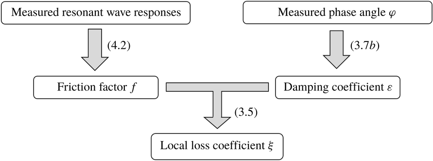
is determined via specifically designed physical model tests. The procedure used to determine the local loss coefficient
 $\unicode[STIX]{x1D709}$
in the present study is illustrated in figure 2. Through physical experiments, the friction factor
 $f$
can be determined by (4.2) with the measured wave resonant responses, and the damping coefficient
 $\unicode[STIX]{x1D700}$
can be obtained based on the measured phase angle through a correlation analysis via (3.7b
). The experiments and the obtained
 $\unicode[STIX]{x1D709}$
values will be described in § 6.
Flowchart of the procedure used to estimate the local loss coefficient
 $\unicode[STIX]{x1D709}$
based on experimental results.

5 Implementation in a linear potential flow model
The present viscous damping model is implemented in a linear potential flow model in the frequency domain, which is the same as that reported by Lu et al. (Reference Lu, Teng, Cheng and Chen2011a ,Reference Lu, Teng, Sun and Chen b ) and suitable for gaps between bodies of different shapes. The higher-order boundary element method (Teng & Eatock Taylor Reference Teng and Eatock Taylor1995) is used in the (modified) potential flow model to solve the boundary value problem formulated in § 2.
Based on the methods proposed for quantifying
 $f$
and
 $\unicode[STIX]{x1D709}$
, an iterative procedure for utilizing (3.5) in the modified potential flow model is proposed below:
(i) For any problem where
$\unicode[STIX]{x1D709}$
is known, start the potential flow computation by setting
$\unicode[STIX]{x1D700}=0$
in (3.5) for a range of frequencies until
$\unicode[STIX]{x1D6EC}_{n}$
is found.(ii) Estimate
$f$
through (4.2) and
$\unicode[STIX]{x1D700}$
through (3.5) based on the results obtained from the previous step. Note that
$\unicode[STIX]{x1D700}$
is dependent on the local flow velocity.(iii) Repeat the computations again with the new
$\unicode[STIX]{x1D700}$
and compare the numerical solutions with the results obtained from the previous step.(iv) If the difference between the wave amplitudes in the gap obtained from two consecutive iterations is smaller than a predetermined norm, stop the iteration.
(v) Otherwise, go back to step (ii) until the iteration has converged.


The above procedure will be demonstrated in § 7.
6 Physical experiments
6.1 Experimental set-up
To quantify
 $\unicode[STIX]{x1D709}$
, physical model tests were conducted in a wave flume 56 m in length, 0.7 m in width, and 0.7 m in depth at Dalian University of Technology, China. An overview of the experimental set-up is shown in figure 3. Two boxes with a draft
 $\overline{d}=0.252~\text{m}$
, gap spacing
 $L_{1}=0.05~\text{m}$
, and breadth
 $\overline{B}=0.5~\text{m}$
were fixed in the wave flume. The width of the models was 0.69 m. The small separations between the two ends of the model and the wave flume walls were less than 0.01 m and were sealed with silicon. The model boxes were fabricated from a 0.01 m-thick plexiglass plate. Six wave gauges (Techco, TWG-600S) were used to measure the wave elevations in the flume. As shown in figure 3, the wave gauge
 $G_{4}$
was located at the centre of the narrow gap, and
 $G_{3}$
and
 $G_{5}$
were arranged 0.05 m in front of the leading Box A and 0.05 m behind the rear Box B, respectively. Since the diameter (0.008 m) of the wave gauges is rather small in comparison with the gap size (0.05 m by 0.7 m), its influence on the surface elevation is expected to be small. To separate the incident wave and the reflected wave, wave gauges
 $G_{1}$
and
 $G_{2}$
were mounted at
 $1~\text{m}+\unicode[STIX]{x1D706}/4$
and 1 m in front of Box A, respectively, where
 $\unicode[STIX]{x1D706}$
denotes the incident wavelength. Wave gauge
 $G_{6}$
was situated 1 m behind the rear Box B. The acquisition rate of the wave gauges was 100 Hz and the absolute error was confirmed to be less than
 $\pm$
1.5 mm based on calibration tests.
Five groups of laboratory tests were performed in this study, in which various edge shapes were considered for the twin boxes, including one sharp corner and four round corners. The edge configuration was measured using a non-dimensional parameter of roundness defined as
 $R=\overline{R}/L_{1}$
, where
 $\overline{R}$
is the radius of the round corner as shown in figure 3. The tested values of the edge roundness
 $R$
were 0, 0.5, 1.0, 2.0 and 3.0, as listed in table 1. For the particular case with sharp corners,
 $R=0$
. Regular waves with a period ranging from 0.90 s to 1.50 s were generated in each group of tests.
An overview of the experimental set-up with a constant body draft
 $\overline{d}=0.252~\text{m}$
, identical body breadth
 $\overline{B}=0.5~\text{m}$
, gap width
 $L_{1}=0.05~\text{m}$
and water depth
 $\overline{h}=0.5~\text{m}$
(
 $d=5.04$
,
 $B=10$
and
 $h=10$
).

Corner radius of the gap entrance.

For each group of tests, approximately 30 incident wave periods were used to capture the equilibrium responses of the wave oscillation in the gap. The tests were terminated before the reflection waves from the wave maker reached the floating boxes. Approximately ten periods of steady-state time series of the free-surface elevation were used to calculate the average amplitude, with the relative root-mean-square error for the amplitude generally less than 4 %. No filtering treatment was conducted on the experimental data. The test repeatability was checked at the beginning and throughout the testing programme. The incident wave height
 $H_{i}$
was initially fixed at 0.024 m (therefore,
 $H_{i}/L_{1}=0.48$
) to identify the resonant frequency
 $\unicode[STIX]{x1D6EC}_{\ast }$
for different
 $R$
values. For this small wave amplitude with
 $H_{i}/\overline{h}=0.048$
, the corresponding wave steepness
 $H_{i}/\unicode[STIX]{x1D706}$
was estimated to be less than 0.02, which falls into the linear wave regime. After the resonant frequency for each of the
 $R$
values was obtained, the incident wave height was varied between
 $H_{i}=0.010~\text{m}$
(
 $H_{i}/L_{1}=0.2$
) and
 $H_{i}=0.045~\text{m}$
(
 $H_{i}/L_{1}=0.9$
) at the identified resonant frequency
 $\unicode[STIX]{x1D6EC}_{\ast }$
for each
 $R$
to investigate the dependence of the resonant amplitude on the incident wave height under the assumption that the resonant frequency is not very sensitive to the incident wave height. The maximum values of
 $H_{i}/\unicode[STIX]{x1D706}$
and
 $H_{i}/\overline{h}$
considered in the tests were 0.027 and 0.09, respectively. This result suggests that several of the incident waves were beyond the linear wave regime.
6.2 Experimental results
6.2.1 Resonant amplitude and frequency
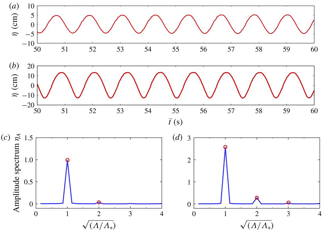
The harmonic components of the steady-state resonant responses in the narrow gap are examined first. A Fourier analysis was performed on the time history of the free-surface elevation measured at
 $G_{4}$
, as illustrated in figure 3. The time series of the free-surface elevation in the gap are shown in figure 4(a,b), and the corresponding amplitude spectra are shown in figure 4(c,d) for the case with
 $R=1.0$
and two incident wave heights
 $H_{i}/L_{1}=0.2$
and 0.9. Special attention was paid to the first and higher harmonic components of the resonant fluid responses in the narrow gap, as shown in figure 4(c,d). Although higher harmonic components were involved, the response was dominated by the first harmonic component. A relatively significant second harmonic component was found for the case shown in figure 4(d), where the largest resonant response amplitude was observed among all the cases considered in this study. The ratio of the amplitude of the second peak to the amplitude of the first peak in figure 4(d) was approximately 0.1, whereas the ratio in figure 4(c) was approximately 0.04.
(a,b) Time series of the free-surface elevations in the gap under resonant conditions for
 $d=5.04$
,
 $B=10$
,
 $R=1.0$
and
 $h=10$
: (a)
 $H_{i}/L_{1}=0.2$
; (b)
 $H_{i}/L_{1}=0.9$
; (c,d) The corresponding non-dimensional amplitude spectra
 $\unicode[STIX]{x1D702}_{A}$
normalized by
 $L_{1}$
for (a,b) with
 $\unicode[STIX]{x1D6EC}_{\ast }(=\unicode[STIX]{x1D70E}_{\ast }^{2}L_{1}/g)$
being the non-dimensional resonant frequency.

The variations of the response amplitude with the incident wave frequency for different gap entrance configurations are presented in figure 5, together with the variations of the relative resonant amplitude and dimensionless mean velocity in the gap with
 $R$
. The wave height and resonant wave height in the gap are denoted by
 $H_{g}$
and
 $H_{g\text{-}Res}$
, respectively. For the purpose of comparison, the previous independent experimental results reported by Saitoh, Miao & Ishida (Reference Saitoh, Miao and Ishida2006) for twin boxes with a sharp-corner entrance are also included in figure 5(a). The two sets of experimental results for the sharp-corner case agree well, with an almost identical resonant frequency of approximately 0.142 and a difference in the resonant wave heights of approximately 3 %.
The relative resonant wave height
 $H_{g\text{-}Res}/H_{i}$
increased dramatically from 4.90 to 7.93 as
 $R$
increased from 0 to 0.5 (see figure 5
b). This substantial increase in the resonant wave height is primarily attributable to the sudden decrease in the system damping
 $\unicode[STIX]{x1D700}$
(as confirmed by the calculated damping coefficients shown in table 2; see details in § 6.2.3). The sudden decrease in
 $\unicode[STIX]{x1D700}$
was likely induced by the disappearance of flow separation at the sharp corners, which in turn caused a significant increase in the flow velocity in the gap as shown in figure 5(b). The resonant frequency only increased slightly as
 $R$
increased from 0 to 0.5.
As
 $R$
increased further from 0.5 to 3.0, the resonant wave height
 $H_{g\text{-}Res}/H_{i}$
decreased slightly. At the largest corner radius of
 $R=3.0$
, the resonant wave height
 $H_{g\text{-}Res}/H_{i}$
decreased to 7.23, and the resonant frequency
 $\unicode[STIX]{x1D6EC}_{\ast }$
increased by approximately 30 % from 0.142 at
 $R=0.5$
to 0.183 at
 $R=3.0$
. The gently decreasing trend of the resonant response amplitude with further increases in
 $R$
beyond
 $R=0.5$
may be due to (i) the weak influence of the roundness
 $R$
on
 $\unicode[STIX]{x1D700}$
for
 $R>0$
, as shown in table 2 or (ii) the decreasing excitation force, as suggested by the increasing natural frequency. The relatively large increase in the resonant frequency with
 $R$
is mainly attributable to the decrease in the fluid mass in the narrow portion of the gap as
 $R$
increases, which leads to an increase in the natural frequency of the system (Moradi et al.
Reference Moradi, Zhou and Cheng2015).
(a) Variation in the relative wave height
 $H_{g}/H_{i}$
in the gap with a non-dimensional incident wave frequency
 $\unicode[STIX]{x1D6EC}(=\unicode[STIX]{x1D70E}^{2}L_{1}/g)$
at various corner radii of
 $R$
for
 $d=5.04$
,
 $B=10$
,
 $h=10$
and
 $H_{i}/L_{1}=0.48$
. Available experimental results from Saitoh et al. (Reference Saitoh, Miao and Ishida2006) at
 $R=0$
are included for comparison. (b) Variation in the relative resonant wave height
 $H_{g\text{-}Res}/H_{i}$
in the gap and non-dimensional resonant free-surface velocity amplitude
 $V_{g\text{-}Res}$
(
 $=|\text{d}\unicode[STIX]{x1D702}(t)/\text{d}t|_{amp}$
) with the corner radius
 $R$
.

6.2.2 Phase angle
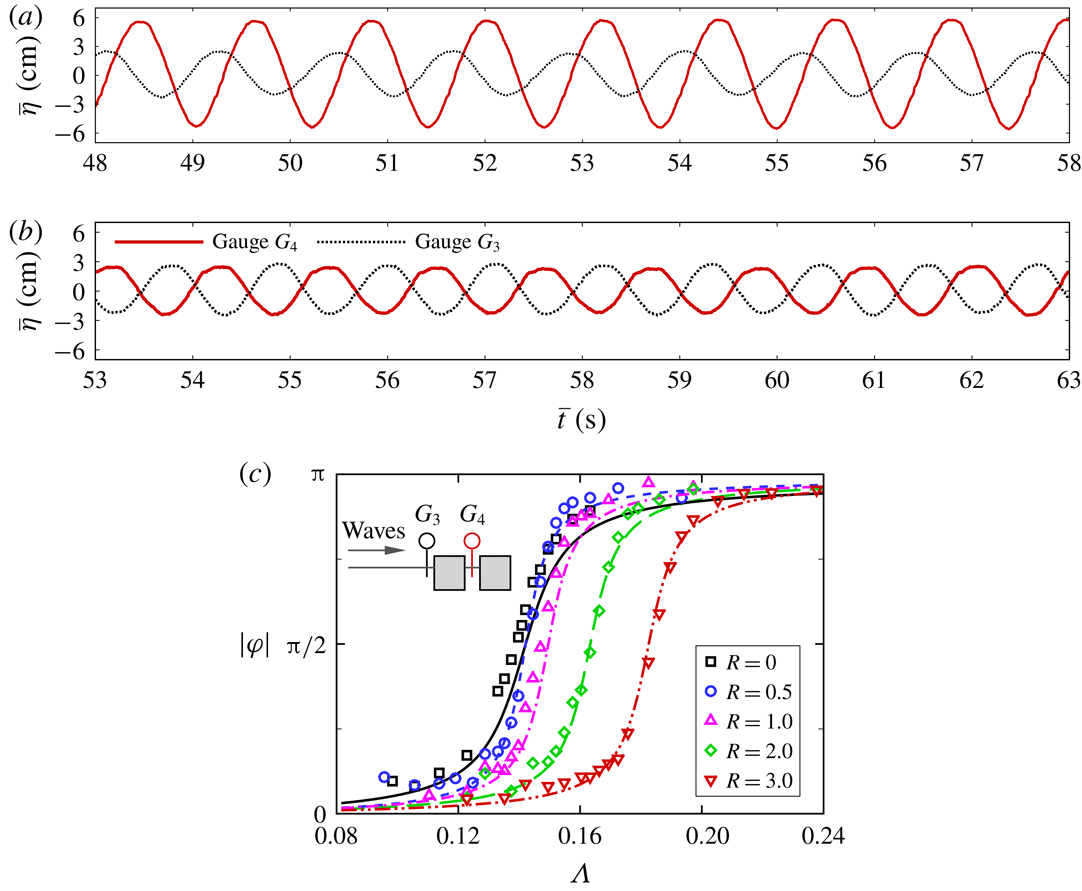
Figure 6(a,b) shows typical examples of the temporal variations of the free-surface elevation measured at the wave gauge locations of
 $G_{3}$
and
 $G_{4}$
, respectively, when the fluid oscillation in the gap was fully developed. Regarding the resonant condition with
 $\unicode[STIX]{x1D6EC}_{\ast }=0.142$
, the wave amplitude in the gap was much larger than that in front of the leading Box A, where a standing wave with an amplitude of
 $1.88H_{i}$
developed. A phase difference of approximately
 $\unicode[STIX]{x03C0}/2$
was observed between the wave oscillations measured at
 $G_{3}$
and
 $G_{4}$
at resonance. In the non-resonant condition with
 $\unicode[STIX]{x1D6EC}=0.163$
, as shown in figure 6(b), the response amplitude in the gap was of the same order of magnitude as that at the front location of the leading box, with a phase difference of approximately
 $\unicode[STIX]{x03C0}$
.
The variations of the phase difference
 $|\unicode[STIX]{x1D711}|$
(absolute value) between the free-surface elevations measured at locations
 $G_{3}$
and
 $G_{4}$
with the incident wave frequency
 $\unicode[STIX]{x1D6EC}$
are shown in figure 6(c). In general, the phase difference increased with the incident wave frequency for all cases. The phase difference
 $|\unicode[STIX]{x1D711}|$
asymptotically approached zero and
 $\unicode[STIX]{x03C0}$
as the incident wave frequency approached zero and infinity, respectively, consistent with the predictions from (3.7b
), in which
 $\unicode[STIX]{x1D700}$
was calibrated through a least-squares analysis, as will be described in the next subsection.
(a,b) Time series of the free-surface elevations in the gap and in front of Box A (corresponding to wave gauges
 $G_{4}$
and
 $G_{3}$
; see figure 3) under different non-dimensional incident wave frequencies for
 $d=5.04$
,
 $B=10$
,
 $R=0$
,
 $h=10$
and
 $H_{i}/L_{1}=0.48$
(sharp-corner case): (a)
 $\unicode[STIX]{x1D6EC}=0.142$
(resonant conditions); (b)
 $\unicode[STIX]{x1D6EC}=0.163$
(non-resonant conditions). (c) Variation in the measured phase difference
 $|\unicode[STIX]{x1D711}|$
(absolute value) with the incident wave frequency
 $\unicode[STIX]{x1D6EC}$
(symbols) for various corner radii
 $R$
. The phase difference is defined as that between the free-surface motions in the gap and in front of Box A. Theoretical predictions were made by (3.7b
), in which
 $\unicode[STIX]{x1D700}$
was calibrated through a least-squares analysis (lines):
 $R=0$
(solid);
 $R=0.5$
(dashed);
 $R=1.0$
(dashed-dot);
 $R=2.0$
(long-dashed);
 $R=3.0$
(dashed-dot-dot).

6.2.3 Damping coefficient
The damping coefficients
 $\unicode[STIX]{x1D700}$
for the tested cases were calibrated against the experimental data through a least-squares-based correlation analysis via (3.7b
). The measured phase differences between the locations at
 $G_{3}$
(in front of the leading box) and
 $G_{4}$
(in the gap) were chosen to calibrate
 $\unicode[STIX]{x1D700}$
because the phase measured at
 $G_{3}$
was representative of the phase angle of the excitation force, based on the numerical results from a CFD model (not shown here). Based on (3.7a
), the difference between
 $\unicode[STIX]{x1D6EC}_{\ast }$
and
 $\unicode[STIX]{x1D6EC}_{n}$
is expected to be negligibly small. Therefore, we calibrated
 $\unicode[STIX]{x1D700}$
via (3.7b
) with the assumption of
 $\unicode[STIX]{x1D6EC}_{n}\approx \unicode[STIX]{x1D6EC}_{\ast }$
. The calibrated results for
 $\unicode[STIX]{x1D700}$
are listed in table 2 with the corresponding correlation coefficients (R-square). The phase differences predicted by (3.7b
) based on the coefficients given in table 2 were compared with the measurements in figure 6(c), and the agreement between the measured and predicted phase differences was reasonable.
Table 2 shows that the damping coefficient
 $\unicode[STIX]{x1D700}$
decreases substantially as the edge shape changes from sharp corners to round corners with a small
 $R=0.5$
. Such a rapid drop in
 $\unicode[STIX]{x1D700}$
was somewhat expected based on our understanding gained from its steady-flow counterpart in pipes with sudden geometrical expansions/constrictions. Moreover, the damping coefficient
 $\unicode[STIX]{x1D700}$
was not very sensitive to the variation in
 $R$
for the round-corner cases (
 $R\geqslant 0.5$
). The results shown in the last column of table 2 also confirmed our earlier speculation that the values of the resonant frequencies and natural frequencies are nearly identical due to the small damping involved in these cases.
Damping coefficient
 $\unicode[STIX]{x1D700}$
for different corner radii
 $R$
.

6.2.4 Local loss and friction coefficients
Further attempts were made to quantify the local loss coefficient
 $\unicode[STIX]{x1D709}$
via the quantification method illustrated in figure 2 based on the
 $\unicode[STIX]{x1D700}$
values presented in table 2 and the friction factors
 $f$
calculated via (4.2). The
 $\unicode[STIX]{x1D709}$
and
 $f$
values are presented in figure 7, which are obtained for a constant incident wave height of
 $H_{i}/L_{1}=0.48$
. As shown in figure 7, for the sharp-corner case, the local loss coefficient
 $\unicode[STIX]{x1D709}$
was approximately 0.95, whereas for the round-corner cases,
 $\unicode[STIX]{x1D709}$
varied between 0.21 and 0.29 with an extremely gentle descending trend for
 $0.5\leqslant R\leqslant 3.0$
. For the friction factor, figure 7 shows that
 $f$
changes little with the increasing corner radius
 $R$
.
The
 $\unicode[STIX]{x1D709}$
values for various edge configurations were also estimated through extrapolations and interpolations of the graphical results presented in Smith & Swift (Reference Smith and Swift2003) and Smith (Reference Smith2004), with the parameters derived from the present experiments. The estimated
 $\unicode[STIX]{x1D709}$
values for the sharp-corner and round-corner cases based on Smith & Swift (Reference Smith and Swift2003) and Smith (Reference Smith2004) are approximately 1.08 and
 $0.2\sim 0.3$
, respectively, largely in agreement with the values estimated based on the present experimental data. Overall, these results provide a certain level of confidence that the damping coefficient of the gap resonance can be obtained by conducting physical model tests systematically for various body geometries.
Local loss coefficient
 $\unicode[STIX]{x1D709}$
and friction factor
 $f$
versus corner radius
 $R$
.

7 Modified potential flow solutions
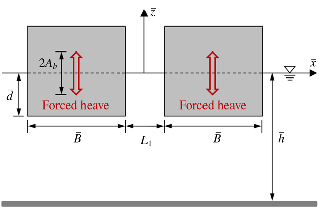
To demonstrate the validity of the present method, the modified potential flow model in the frequency domain was used to simulate the present experimental cases and those of the moonpool resonance problems presented in Faltinsen & Timokha (Reference Faltinsen and Timokha2015). The simulations were performed based on the predetermined damping coefficients. The first test case was the example presented in Faltinsen et al. (Reference Faltinsen, Rognebakke and Timokha2007) with
 $\unicode[STIX]{x1D709}$
and
 $f$
determined based on (3.6) and (4.2), respectively. Figure 8 shows a sketch of the experimental set-up of Faltinsen et al. (Reference Faltinsen, Rognebakke and Timokha2007), where a rectangular moonpool is under forced heave motions with an amplitude
 $A_{b}$
. Their flume model tests were carried out for a range of forcing frequencies
 $\unicode[STIX]{x1D6EC}$
, with three different geometric configurations, corresponding to the dimensionless parameters (normalized by
 $L_{1}$
) in table 3.
Sketch of the experimental set-up of Faltinsen et al. (Reference Faltinsen, Rognebakke and Timokha2007).

Geometric parameters and forcing amplitude
 $(A_{b}/L_{1})$
of the model tests of Faltinsen et al. (Reference Faltinsen, Rognebakke and Timokha2007).

The numerical results for the excited piston-mode fluid response are shown in figure 9, where
 $A_{g}$
denotes the amplitude of the piston-mode wave oscillations in the moonpool. The presented predictions agree well with the experimental results by Faltinsen & Timokha (Reference Faltinsen and Timokha2015). The predicted resonant amplitudes are generally lower than the semi-analytical solutions (with damping) of Faltinsen & Timokha (Reference Faltinsen and Timokha2015).
The ratio of the friction-induced damping force to that due to flow separation, denoted by
 $E_{r}$
, was evaluated based on (3.2). The results are detailed in table 4 for the cases shown in figure 9. The contribution of the damping force from the wall friction was generally less than 9 % of the flow separation for the cases investigated in Faltinsen & Timokha (Reference Faltinsen and Timokha2015). Thus, the numerical results would not be significantly affected even though the loss due to friction is completely ignored. As confirmation, the calculations were repeated by artificially setting
 $f=0$
, and the results are shown as dotted (green) lines in figure 9. The influence of the wall friction forces on the numerical results was indeed small. This influence would likely become more significant if the draft
 $d$
is increased. The contribution from the friction loss will be further discussed later in this section.
Comparison of the present predictions and previous results for the relative wave amplitude
 $A_{g}/A_{b}$
in a moonpool undergoing heave motions. The geometric parameters and forcing amplitudes
 $(A_{b}/L_{1})$
of the experiments of Faltinsen et al. (Reference Faltinsen, Rognebakke and Timokha2007) are shown in table 3. (a) Case 1
 $a$
; (b) case 1
 $b$
; (c) case 2
 $a$
; (d) case 2
 $b$
; (e) case 3. The experimental results are taken from Faltinsen & Timokha (Reference Faltinsen and Timokha2015) (▫, red) and were filtered by the reflection waves. The semi-analytical solutions with/without artificial damping are taken from Faltinsen & Timokha (Reference Faltinsen and Timokha2015) (long-dashed/dashed-dot). The present modified potential solutions with iterations are based on (3.5) (solid and dotted lines), where
 $\unicode[STIX]{x1D709}$
is estimated based on (3.6), in which the coefficients
 $K(Sn,K_{c})$
and
 $b_{\ast }$
are determined according to the method of Faltinsen & Timokha (Reference Faltinsen and Timokha2015);
 $f$
is estimated by (4.2) for the solid lines (——), and
 $f$
is artificially set at
 $f=0$
for the dotted lines (
 $\cdots \cdots$
).

Estimated ratio of the friction-induced damping force to that due to flow separation (denoted by
 $E_{r}$
) for the cases shown in figure 9.

The modified potential flow model was also applied to the flume test cases reported in this study. The numerical results are compared with the experimental data in figure 10. The present numerical results agree reasonably well with the experimental measurements, whereas the conventional potential flow model without the damping term over-predicts the resonant response amplitudes significantly. The relative differences in the resonant frequency
 $\unicode[STIX]{x1D6EC}_{\ast }$
and resonant wave height
 $H_{g\text{-}Res}/H_{i}$
were less than 4 % and 15 %, respectively. For comparison, with the aid of (3.6), the pressure drop coefficient
 $K(Sn,K_{c})$
proposed by Faltinsen & Timokha (Reference Faltinsen and Timokha2015) was directly applied to compute those cases, and the results are shown in figure 10 as dashed-dot (green) lines. The method proposed by Faltinsen & Timokha (Reference Faltinsen and Timokha2015) worked extremely well for the sharp-corner case but under-predicted the response amplitude for the round-corner cases in which the viscous damping was much smaller than that in the sharp-corner case.
Comparison of the numerical predictions of the potential flow models (with/without the damping term) and the experimental results for
 $d=5.04$
,
 $B=10$
,
 $h=10$
and
 $H_{i}/L_{1}=0.48$
. Cases with both sharp and round corners are considered: (a)
 $R=0$
; (b)
 $R=0.5$
; (c)
 $R=1.0$
; (d)
 $R=2.0$
; (e)
 $R=3.0$
. Experimental results (▫, red); linear potential solutions without the damping term (dashed line - - - -); modified potential solutions with the damping coefficient
 $\unicode[STIX]{x1D700}$
listed in table 2 (solid line ——); modified potential solutions with iterations based on (3.5) (dashed-dot line – ⋅ – ⋅ –), where
 $\unicode[STIX]{x1D709}$
was approximated by (3.6), in which the coefficients
 $K(Sn,K_{c})$
and
 $b_{\ast }$
were determined by the method of Faltinsen & Timokha (Reference Faltinsen and Timokha2015), and
 $f$
was estimated by (4.2).

The sensitivity of the numerical results to the choice of the local loss coefficient
 $\unicode[STIX]{x1D709}$
was examined by applying the
 $\unicode[STIX]{x1D709}$
value determined with a constant incident wave height of
 $H_{i}=0.024~\text{m}$
(
 $H_{i}/L_{1}=0.48$
) to a range of cases with different incident wave heights at each of the
 $R$
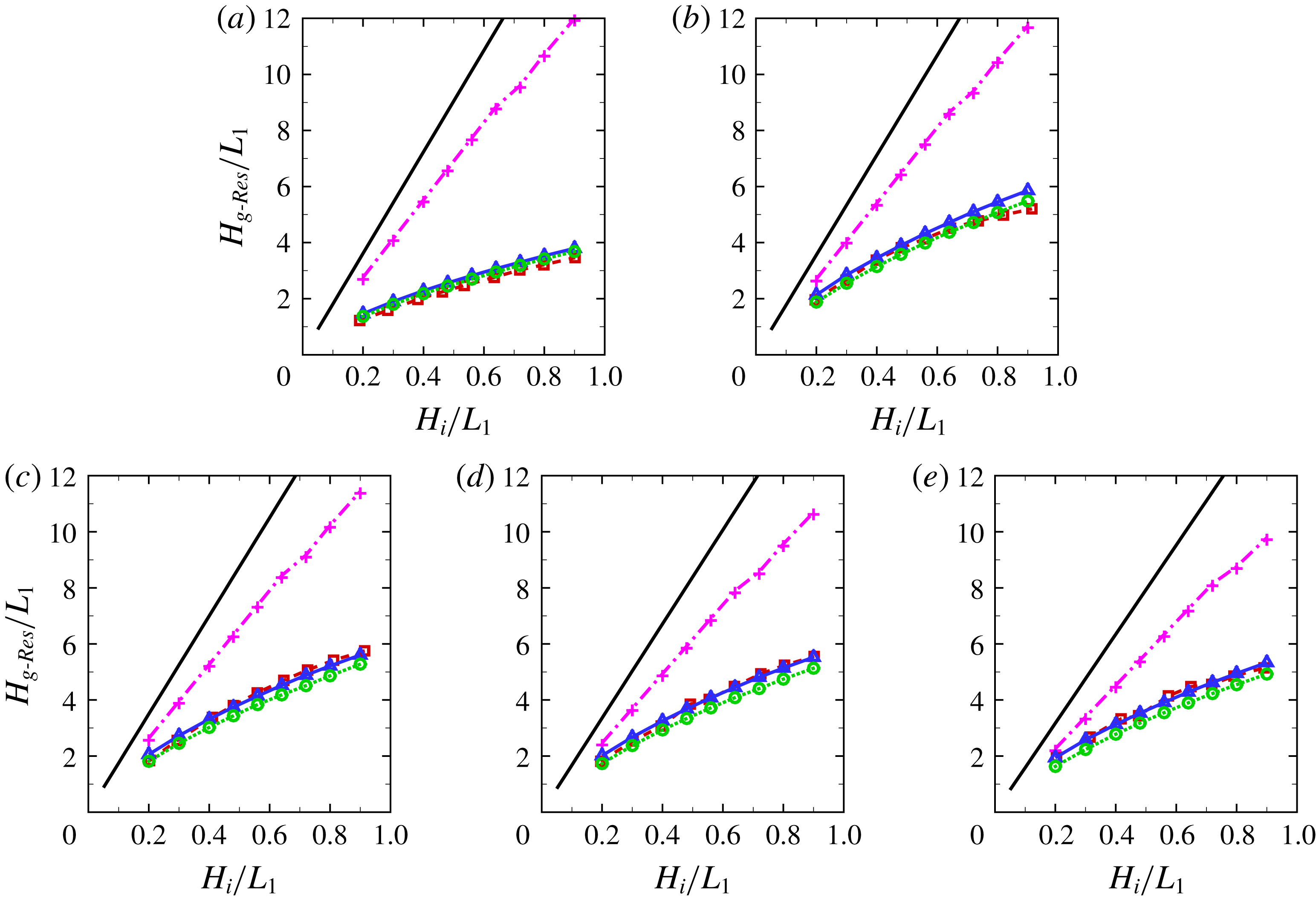
values investigated in this study. The numerical results are compared with the experimental data from this work in figure 11. To further examine the individual effects of the friction and local loss components of viscous damping on the numerical results, four different sets of numerical results are included in figure 11: (i)
 $f=0$
and
 $\unicode[STIX]{x1D709}=0$
(without damping), (ii)
 $f\neq 0$
and
 $\unicode[STIX]{x1D709}=0$
(with friction damping only), (iii)
 $f=0$
and
 $\unicode[STIX]{x1D709}\neq 0$
(with local flow separation damping only) and (iv)
 $f\neq 0$
and
 $\unicode[STIX]{x1D709}\neq 0$
(with both friction and flow separation damping). The conventional linear potential model over-predicted the resonant amplitude, particularly for the cases with large incident wave amplitudes. The numerical results with
 $f\neq 0$
and
 $\unicode[STIX]{x1D709}=0$
worked relatively well only in the round-corner cases with a large corner radius (
 $R=2.0$
and 3.0) and a small incident wave amplitude (
 $H_{i}/L_{1}=0.2$
). These results are possibly due to (i) the insignificance (relative to the friction loss) of the local energy loss induced by small-amplitude incident waves for the round-corner cases because this loss is quadratically proportional to the mean flow velocity (which is a small quantity
 ${<}$
1.0; see figure 5
b) in the gap; by contrast, the friction loss is linearly proportional to the mean flow velocity; and (ii) the local energy loss in the case with sharp corners was significant, even at small amplitudes of incident waves, due to the flow separation expected at the sharp-corner locations. The numerical model with
 $f\neq 0$
and
 $\unicode[STIX]{x1D709}=0$
significantly over-predicted the resonant response amplitude for all other cases with relatively large incident wave amplitudes because the local loss dominated the friction loss in those cases. As shown in figure 11, the resonant amplitude predicted by using
 $f\neq 0$
and
 $\unicode[STIX]{x1D709}=0$
was almost linearly proportional to the incident wave height for the entire range of incident wave heights considered in this study. This result suggests that the boundary layer flow over the side walls of the gap was in the laminar regime, as indicated by (4.3), where the shear stress on the side walls is linearly proportional to the mean velocity in the gap. This point will be further elaborated on when the results shown in figure 12 are discussed.
The numerical results with
 $f=0$
and
 $\unicode[STIX]{x1D709}\neq 0$
generally agree well with the experimental results for all cases investigated here, suggesting that the local loss dominated the friction loss, particularly for the case with sharp corners, where flow separation was expected. A general trend in figure 11 is that the differences between the experimental measurements and the numerical results with
 $f=0$
and
 $\unicode[STIX]{x1D709}\neq 0$
increased with the incident wave height
 $H_{i}/L_{1}$
. This behaviour was not necessarily caused by the dependence of
 $\unicode[STIX]{x1D709}$
on the Keulegan–Carpenter number
 $K_{c}$
. Instead, it was induced by the omission of the friction contribution (
 $f=0$
), because this trend disappeared in the numerical results with
 $f\neq 0$
and
 $\unicode[STIX]{x1D709}\neq 0$
. These observations suggest that
 $\unicode[STIX]{x1D709}$
is relatively insensitive to the incident wave height for the range of incident wave heights investigated here.
As expected, the numerical results with
 $f\neq 0$
and
 $\unicode[STIX]{x1D709}\neq 0$
generally agreed better with the experimental results than all other artificial cases with either the local loss coefficient or friction coefficient being deliberately set to zero, except in the cases with the largest three
 $R$
values investigated in this study (figure 10
c–e). Although the underlying causes might be diverse (and are not further explored due to certain limitations), these results might be due to the errors introduced in estimating the friction contribution based on the empirical formulae (4.1)–(4.3) and the simplification made in the derivation of (3.4), where the draft of the gap is assumed to be
 $d$
even for the cases with round corners. Strictly speaking, (4.1)–(4.3) are only applicable for oscillatory flow parallel to a flat surface. The flow in the gap entrance region was neither necessarily parallel to the surface, nor was the surface flat. Such an effect was more pronounced for large
 $R$
values because the wall friction contribution to the overall damping was more pronounced than that in the other cases investigated here.
Comparison of the numerical predictions and experimental results for the resonant wave height
 $H_{g\text{-}Res}/L_{1}$
with different incident wave heights
 $H_{i}/L_{1}$
and various corner radii: (a)
 $R=0$
; (b)
 $R=0.5$
; (c)
 $R=1.0$
; (d)
 $R=2.0$
; (e)
 $R=3.0$
, for
 $d=5.04$
,
 $B=10$
,
 $h=10$
. Experimental results (- - ▫ - -); linear potential flow solution without any damping term (——); modified potential solution considering viscous damping due to wall friction only (artificially setting
 $f\neq 0$
and
 $\unicode[STIX]{x1D709}=0$
) (–
 $+$
–); modified potential solution considering damping due to flow separation only (
 $f=0$
and
 $\unicode[STIX]{x1D709}\neq 0$
) (–▵–); and modified potential solution considering damping due to both flow separation and wall friction (
 $f\neq 0$
and
 $\unicode[STIX]{x1D709}\neq 0$
) (

 $\unicode[STIX]{x1D709}$
can be found in figure 7, and
 $f$
was estimated by (4.2).
Smith & Swift (Reference Smith and Swift2003) suggested that
 $\unicode[STIX]{x1D709}$
is generally dependent on the Reynolds number
 $Re$
and the Keulegan–Carpenter number
 $K_{c}$
, defined as
 $K_{c}=\overline{V}_{g}T/2\overline{R}$
, with
 $\overline{V}_{g}$
the amplitude of the oscillating velocity in the gap (the overbars imply dimensional values), for oscillatory flow through a geometry similar to the one investigated in this study. The ranges of
 $Re$
and
 $K_{c}$
covered in this study are quantified in figure 12. Note that the
 $K_{c}$
values for the sharp-corner cases are not included in figure 12(a) due to the adopted definition of
 $K_{c}$
from Smith & Swift (Reference Smith and Swift2003) with
 $\overline{R}$
as a denominator. Figure 12(a) shows that
 $K_{c}$
reached a maximum value of 16.4 at
 $H_{i}/L_{1}=0.9$
with
 $R=0.5$
and approached the minimum value of 1.0 at
 $H_{i}/L_{1}=0.2$
with
 $R=3.0$
in the present experiments. As shown in figure 12(b), the minimum
 $Re$
was
 $5\times 10^{3}$
at
 $H_{i}/L_{1}=0.2$
with
 $R=0$
, and the maximum
 $Re$
was approximately
 $10^{5}$
at
 $H_{i}/L_{1}=0.9$
with
 $R=1.0$
. These results confirm that the boundary layer flow over the side walls of the gap was in the laminar regime because the maximum
 $Re$
was smaller than
 $5\times 10^{5}$
.
(a) Variation in the Keulegan–Carpenter number
 $K_{c}$
(
 $=\overline{V}_{g}T/$
 $2\overline{R}$
) with the incident wave height
 $H_{i}/L_{1}$
and corner radius
 $R$
(corresponding to the experimental results in figure 11) for
 $d=5.04$
,
 $B=10$
,
 $h=10$
; (b) the same as (a) but for the Reynolds number
 $Re$
(defined in (4.2)).

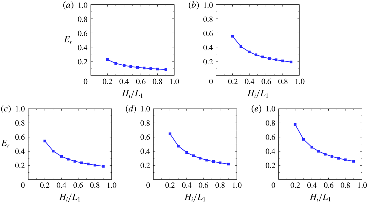
The contributions from the wall friction damping for the cases shown in figure 11 were further examined by quantifying the ratio of the friction and flow separation components of the viscous damping. The ratio of the friction-induced damping force to that due to flow separation, denoted by
 $E_{r}$
, was evaluated based on (3.2) The estimated
 $E_{r}$
values for different incident wave heights and
 $R$
values are shown in figure 13;
 $E_{r}$
generally decreased with the increasing incident wave height because the damping forces associated with local and friction energy losses are quadratically and linearly proportional to the mean velocity in the gap, respectively. As the wave height increased, the local energy loss increased much faster than the energy loss due to the wall friction;
 $E_{r}$
was less than 0.3 for the sharp-corner cases and as high as 0.8 for the case with the largest
 $R=3.0$
and the smallest
 $H_{i}/L_{1}=0.2$
. The results shown in figure 13 suggest that the contribution from the wall friction forces to the overall viscous damping could be substantial, particularly for the cases with large round edges and small incident wave amplitudes.
Estimated ratio of the friction-induced damping force to that due to flow separation
 $E_{r}$
(corresponding to numerical results of ‘
 $f\neq 0$
and
 $\unicode[STIX]{x1D709}\neq 0$
’ in figure 11) with different incident wave heights
 $H_{i}/L_{1}$
and various corner radii: (a)
 $R=0$
; (b)
 $R=0.5$
; (c)
 $R=1.0$
; (d)
 $R=2.0$
; (e)
 $R=3.0$
, for
 $d=5.04$
,
 $B=10$
,
 $h=10$
. The numerical solutions are based on the modified potential flow model with the damping coefficient
 $\unicode[STIX]{x1D700}$
estimated by (3.5) via the iterative method. The values of the local loss coefficient
 $\unicode[STIX]{x1D709}$
are shown in figure 7, and
 $f$
was calculated by (4.2).

8 Discussion
8.1 On estimating the frictional damping force
In additional to the simplified formula (3.2), the viscous damping force due to the wall friction can be evaluated in a more general and rigorous manner (Molin et al.
Reference Molin, Remy, Kimmoun and Stassen2002). First, the dissipated energy due to the wall friction over one period
 $T$
is given by
 $$\begin{eqnarray}\displaystyle \overline{E}_{f}=\int _{0}^{\overline{S}_{b}}\left(\int _{0}^{T}\unicode[STIX]{x1D70C}\frac{f}{2}(\overline{V}_{t}(\overline{S})\cos (\unicode[STIX]{x1D70E}\overline{t}-\unicode[STIX]{x1D711}))^{2}\,\text{d}\overline{t}\right)\text{d}\overline{S}=\int _{0}^{\overline{S}_{b}}\frac{\unicode[STIX]{x1D70C}\unicode[STIX]{x03C0}f}{2\unicode[STIX]{x1D70E}}(\overline{V}_{t}(\overline{S}))^{2}\,\text{d}\overline{S}, & & \displaystyle\end{eqnarray}$$
where
 $\overline{V}_{t}(\overline{S})$
is the amplitude of the tangent oscillating velocity on the wet surface of the boxes, as illustrated in figure 14, and
 $\overline{S}_{b}$
is the total length of the wet surface lines of the boxes (corresponding to the red lines). In (8.1),
 $\overline{V}_{t}(\overline{S})$
, which is difficult to measure directly in experiments, can be obtained based on potential flow solutions. Apart from (8.1), the frictional energy loss can also be evaluated by
 $$\begin{eqnarray}\displaystyle \overline{E}_{f}=\int _{0}^{T}\overline{F}_{d-f}\cos (\unicode[STIX]{x1D70E}\overline{t}-\unicode[STIX]{x1D711})\cdot \overline{V}_{g}\cos (\unicode[STIX]{x1D70E}\overline{t}-\unicode[STIX]{x1D711})\,\text{d}\overline{t}=\frac{\unicode[STIX]{x03C0}\overline{F}_{d-f}\overline{V}_{g}}{\unicode[STIX]{x1D70E}}, & & \displaystyle\end{eqnarray}$$
where
 $\overline{F}_{d-f}$
is the amplitude of the frictional damping force and
 $\overline{V}_{g}$
is the amplitude of the oscillating velocity in the gap. Based on (8.1) and (8.2), the frictional damping force can be written as
 $$\begin{eqnarray}\displaystyle \overline{F}_{d-f}\cos (\unicode[STIX]{x1D70E}\overline{t}-\unicode[STIX]{x1D711})=\frac{\displaystyle \int _{0}^{\overline{S}_{b}}\unicode[STIX]{x1D70C}f(\overline{V}_{t}(\overline{S}))^{2}\,\text{d}\overline{S}}{2\overline{V}_{g}}\cos (\unicode[STIX]{x1D70E}\overline{t}-\unicode[STIX]{x1D711}). & & \displaystyle\end{eqnarray}$$
Compared with (3.2), (8.3) is a more general and rigorous method for estimating the frictional damping force.
Sketch for estimating the frictional damping force based on potential flow solutions.

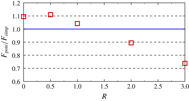
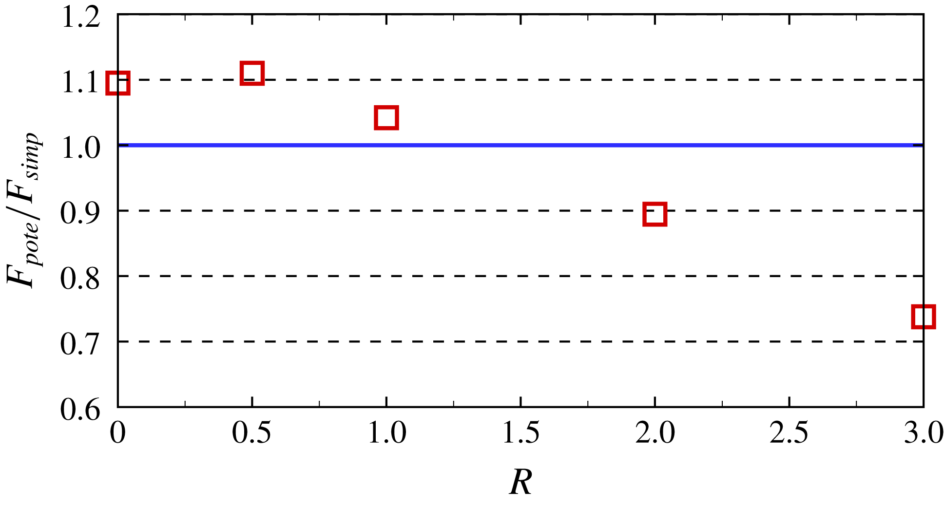
Under resonant conditions, the estimated frictional damping forces based on the two methods ((8.3) and (3.2)) for the sharp- and round-corner cases are shown in figure 15. The result based on (8.3) and linear potential flow solutions is denoted by
 $F_{pote}$
, and that estimated by the simplified method based on (3.2) is denoted by
 $F_{simp}$
. Figure 15 shows that
 $F_{pote}/F_{simp}$
is between 0.90 and 1.11 for
 $R\leqslant 2$
, suggesting that the approximation made in (3.2) is reasonably good for
 $R\leqslant 2$
. The largest difference between
 $F_{pote}$
and
 $F_{simp}$
appears in the case with the largest corner radius (
 $R=3.0$
) investigated in the present study, corresponding to
 $F_{pote}/F_{simp}=0.74$
. It is recommended that (8.3) is used in situations where
 $R>2.0$
.


8.2 Extensions of the viscous damping model
In additional to the present two identical bodies subjected to water waves, the viscous damping model can be applied in two-dimensional cases with different geometries of bodies and wave conditions as long as the local loss coefficient in the model is quantified. However, in its present form, this viscous damping model is only suitable for piston-mode responses with fixed structures. Considerable research efforts are required for extensions to problems involving moving bodies and three-dimensional problems where multiple response modes exist. For a floating body with significant motion, the relative velocity between the bodies and fluid should be considered in estimating the frictional damping force. For three-dimensional problems, the frictional damping force should be estimated through the integration method described by (8.3). Furthermore, both body motions and three-dimensional effects may influence the viscous damping due to flow separation. Hence, the local loss coefficient must be quantified under corresponding conditions. When multiple response modes exist, it may require conducting a dynamic analysis to determine the response modes in which viscous damping plays an important role.
9 Summary and conclusions
This study considers the piston-mode fluid resonance in a moonpool or the narrow gap formed by two fixed boxes. In §§ 2–5, after the statement of the problem, we introduced a modified potential flow model and a viscous damping model, presented the implementation of the viscous damping model in the (modified) potential flow model and reported quantification methods for the local and friction loss coefficients in the model. In § 6, we reported the physical experiments, and the local loss coefficient was quantified based on the measured phase difference. In § 7, the (modified) potential flow model implemented with the viscous damping model was used to predict the resonant response in a narrow gap/moonpool. Numerical predictions were carried out for varied damping conditions and compared with the available experimental and numerical data in the literature and the present experimental results. In § 8, a more general and rigorous method for estimating the frictional damping force is presented. The extensions of the present methodology to more general situations are also discussed.
A viscous damping model for energy losses due to both wall friction and flow separation is proposed for a two-dimensional fluid response in a narrow gap or moonpool. An equivalent linearized viscous damping coefficient (
 $\unicode[STIX]{x1D700}$
) dependent on the body geometries, response amplitude, natural frequency and surface roughness is devised to account for the energy dissipation. The damping component associated with the flow separation
 $(\unicode[STIX]{x1D709})$
is determined through a correlation analysis of the experimental data obtained in this study, and the friction component
 $(f)$
is calculated using a well-established empirical formula. The application of the proposed viscous damping model in the frame of potential flow theory leads to a modified potential flow model that can predict the amplitude of the piston-mode resonance for a wide range of flow conditions without artificially tuning the damping coefficient, including a sharp/round gap entrance corner and various incident wave amplitudes. Further evidence from specifically designed physical tests indicates that the viscous damping due to wall friction plays an important role for round-corner gap entrance geometries and small incident wave heights.
The physical model tests conducted in this work confirm that the gap geometries significantly influence the resonant response amplitude and resonant/natural frequency of the fluid trapped in the gap. The resonant wave amplitude becomes much higher when the shape of the gap entrance changes from a sharp corner to a round corner.
Despite the developments in this work, the method proposed by Faltinsen & Timokha (Reference Faltinsen and Timokha2015) can be extended to cases with a round gap entrance if an appropriate pressure drop coefficient is adopted. Both methods shed light on the successful prediction of resonance problems within the modified potential flow model without artificially tuning the damping coefficient. The proposed viscous damping model can also be applied in other modified potential flow models, such as that of Chen (Reference Chen2004).
Acknowledgements
This work is supported by the NSFC under grant no. 51490673 and the National Key R&D Program of China (2016YFE0200100). L.C. would like to acknowledge support from the Australian Research Council through ITRH programme grant IH140100012.