



1. Introduction
A thermogravitational column (TGC) consists of a cavity (parallelepipedal or cylindrical) filled with fluid and subjected to a temperature difference perpendicular to gravity. Buoyancy-driven flows induced by horizontal temperature gradients have been studied since the seminal work of Hadley (Reference Hadley1735), who first described fluid motion driven by gravitational effects in laterally heated systems. Later hydrodynamic formulations of this configuration, commonly referred to as Hadley or Birikh flow, established the basic reference state for thermally driven convection under horizontal temperature gradients (Birikh 1966). Comprehensive theoretical descriptions of such buoyancy-driven flows and their stability properties can be found in classical monographs such as those by Gershuni & Zhukhovitskii (Reference Gershuni and Zhukhovitskii1976) and Getling (Reference Getling1998), which provide the conceptual framework underlying more complex configurations, including the binary mixture systems considered here. In such systems confined in a TGC, this temperature difference induces a horizontal concentration gradient through the thermodiffusion phenomenon, while molecular diffusion acts to homogenise the mixture. The resulting horizontal density difference drives thermogravitational convection, enhancing species separation along the cavity height. For positive thermodiffusion coefficients, a stable linear density stratification is established. Under certain assumptions, Furry, Jones & Onsager (Reference Furry, Jones and Onsager1939) (FJO) derived an analytical expression for the steady-state dimensional vertical concentration gradient (
 ${\partial c^*}/{\partial z^*}$
), being
 \begin{equation} \frac {\partial c^*}{\partial z^*}= -504c^*_0 \big(1-c^*_0\big)\frac {\nu }{e^4\beta _{\textit{T}} g}D_T. \end{equation}
In (1.1)
 $g$
,
 $\nu$
,
 $\beta _{\textit{T}}$
,
 $c^*_0$
,
 $D_T$
and
 $e$
are the gravitational acceleration, the kinematic viscosity, the thermal expansion coefficient, the mass fraction of the densest component corresponding to the temperature
 $ T_0^*$
, the thermodiffusion coefficient and the width of the cavity gap. Thus, (1.1) has been widely used to determine positive
 $D_T$
coefficients of binary mixtures by experimentally measuring
 $\partial c^*/\partial z^*$
.
Conversely, a negative thermodiffusion coefficient generates an adverse density gradient that is dynamically unstable, as the denser component migrates towards the hot region and accumulates in the upper part of the cavity. Growing scientific interest has emerged in understanding the thermogravitational stability problem associated with negative
 $D_T$
coefficients due to its fundamental and practical relevance. Analytically and numerically, several studies have addressed this issue. Batiste, Alonso & Mercader (Reference Batiste, Alonso and Mercader2004) showed that binary mixtures with negative
 $D_T$
coefficients remain stable to two-dimensional perturbations but become unstable to three-dimensional disturbances. Zebib (Reference Zebib2007) first examined two-dimensional stability and later extended the analysis to three-dimensional disturbances (Zebib 2008), providing correlations for the onset of both longitudinal and transverse instabilities. Ryzhkov & Shevtsova (Reference Ryzhkov and Shevtsova2009b
) analysed long-wave perturbations and subsequently broadened the study to include three-dimensional disturbances, thereby covering a wider range of conditions (Ryzhkov & Shevtsova Reference Ryzhkov and Shevtsova2009a
).
All the above-mentioned works assumed that the TGC is infinite along the horizontal axis perpendicular to the temperature gradient, thereby neglecting the effects of lateral confinement. However, such confinement can significantly influence both stability conditions and the magnitude of species separation. Numerical simulations with negative
 $D_T$
performed by Seta et al. (Reference Seta, Gavalda, Bou-Ali and Ruiz2020) in Cartesian TGCs and by Kozlova, Ryzhkov & Bou-Ali (Reference Kozlova, Ryzhkov and Bou-Ali2021) in cylindrical TGCs indicated that reducing the lateral aspect ratio
 $B$
(or the ratio of cylinder radii in the cylindrical case) may stabilise the adverse density gradient. In cylindrical configurations, Bou-Ali et al. (Reference Bou-Ali, Ecenarro, Madariaga, Santamaría and Valencia1999) experimentally achieved stabilisation of a binary mixture with a negative
 $\psi$
, depending on the applied temperature difference, and subsequently reported the first measurements of
 $D_T$
for negative mixtures (Bou-Ali et al. 2000). More recently, Sanjuan et al. (Reference Sanjuan, Ali Ammar, Hirata, Ouarzazi, M. and Bou-Ali2025) presented a three-dimensional theoretical analysis of how transverse confinement in Cartesian TGCs affects steady-state species separation, showing that
 \begin{equation} \frac {\Delta c^*_{\text{3D}}}{\Delta c^*_{\textit{FJO}}}=\frac {a_{\psi }(B)}{ \frac {9!}{(Le\,{\textit{Ra}}_{\textit{T}})^2}+a_{\textit{c}}(B)}. \end{equation}
The functions
 $a_{{\psi }}(B)$
and
 $a_{\textit{c}}(B)$
involve integrals of
 $x$
- and
 $y$
-dependent series and their explicit expressions are given in Sanjuan et al. (Reference Sanjuan, Ali Ammar, Hirata, Ouarzazi, M. and Bou-Ali2025). They represent the correction factors due to the transversal confinement of the cavity with
 $a_{\psi }(B) = a_{\textit{c}}(B) = 1$
in the limit of infinite
 $B$
. We emphasise that in this limit and assuming
 ${9!}/{(Le\,{\textit{Ra}}_{\textit{T}})^2} \ll 1$
, the expression of separation
 $\Delta c^*_{\textit{FJO}}$
(1.1) obtained by Furry et al. (Reference Furry, Jones and Onsager1939) is recovered. Otherwise, as reported in Sanjuan et al. (Reference Sanjuan, Ali Ammar, Hirata, Ouarzazi, M. and Bou-Ali2025), (1.2) reveals that the steady-state species separation for stable configurations with positive
 $D_T$
increases by reducing the transversal aspect ratio
 $B$
.
Motivated by the experimental work of Bou-Ali et al. (Reference Bou-Ali, Ecenarro, Madariaga, Santamaría and Valencia1999), by the numerical results obtained by Seta et al. (Reference Seta, Gavalda, Bou-Ali and Ruiz2020) and Kozlova et al. (Reference Kozlova, Ryzhkov and Bou-Ali2021), and by the theoretical, numerical and experimental results of Sanjuan et al. (Reference Sanjuan, Ali Ammar, Hirata, Ouarzazi, M. and Bou-Ali2025), the present work aims to study the effect of the transverse aspect ratio of the cavity on the three-dimensional stability of species separation in binary mixtures with a negative thermodiffusion coefficient considering Cartesian TGCs.
The paper is structured as follows. Section 2 presents the physical description of the problem and the basic state derived in Sanjuan et al. (Reference Sanjuan, Ali Ammar, Hirata, Ouarzazi, M. and Bou-Ali2025). Section 3 addresses the linear stability analysis. Sections 4 and 5 describe, respectively, numerical simulations of the fully nonlinear three-dimensional problem and the experimental investigations. Finally, the conclusions are presented in § 6.
2. Physical problem and review of the basic state
A binary fluid mixture confined in a vertical slot of height
 $H$
, thickness
 $e$
and width
 $b$
is considered. A difference of temperature
 $\Delta T^*$
is maintained between both vertical boundaries, the temperature on the right-hand wall being higher than that on the left-hand wall. The horizontal plates at
 $z^*=\pm ({H}/{2})$
and the lateral plates at
 $y^*=\pm ({b}/{2})$
are assumed adiabatic and all the boundaries are rigid and impermeable to mass fluxes. Furthermore, the vertical slot is supposed to have a large aspect ratio height/thickness (
 $ A=H/e$
) and finite transversal aspect ratio width/thickness (
 $ B=b/e$
). The physical fields are made dimensionless by choosing
 $e$
,
 $b$
and
 $H$
for coordinates
 $x^*$
,
 $y^*$
and
 $z^*$
respectively,
 $({e^2}/{\kappa })$
for time,
 $({\kappa }/{e})$
for velocity,
 $({\mu \kappa })/{e^2}$
for pressure,
 $\Delta T^*$
for the temperature difference
 $T^*-T_0^*$
and
 $({\beta _{\textit{T}} \Delta T^*}){/\beta _{\textit{C}}}$
for the concentration difference
 $c^*-c_0^*$
.
Thus, in non-dimensional form the governing equations are
 \begin{align} &\qquad \quad \boldsymbol{\nabla }\boldsymbol{\cdot }\boldsymbol{u}=0,\end{align}
 \begin{align} \frac {\partial \boldsymbol{u}}{\partial t}+( \boldsymbol{u} \boldsymbol{\cdot }\boldsymbol{\nabla }) \boldsymbol{u} =&-\textit{Pr} \boldsymbol{\nabla }P+\textit{Pr} {\textit{Ra}}_{\textit{T}}(T-c) \boldsymbol{e}_z+Pr \boldsymbol{\nabla} ^2 \boldsymbol{u}, \end{align}
 \begin{align} &\quad \frac {\partial T}{\partial t}+ \boldsymbol{u} \boldsymbol{\cdot }\boldsymbol{\nabla }T = \boldsymbol{\nabla} ^{2} T,\end{align}
 \begin{align} \frac {\partial c}{\partial t}+&\boldsymbol{u} \boldsymbol{\cdot }\boldsymbol{\nabla }c =\frac {1}{\textit{Le}}\big(\boldsymbol{\nabla} ^{2}c+\psi \boldsymbol{\nabla} ^{2} T\big). \end{align}
The boundary conditions can be expressed as
 \begin{align}&\quad {u}= {0}\;\;\text{at}\;\;x=\pm \frac {1}{2},\quad y=\pm \frac {1}{2} \quad \text{and} \quad z=\pm \frac {1}{2}, \end{align}
 \begin{align}&\qquad T=\frac {1}{2}\;\;\text{at}\;\;x= \frac {1}{2}\;\;\;\;\text{and} \;\;\;\; T=-\frac {1}{2}\;\;\text{at}\;\;x= - \frac {1}{2}, \end{align}
 \begin{align}&\qquad\qquad\quad \frac {\partial c}{\partial x}+\psi \frac {\partial T}{\partial x}=0\;\;\text{at}\;\;x=\pm \frac {1}{2}, \end{align}
 \begin{align}& \frac {\partial T}{\partial z}= \frac {\partial c}{\partial z}= 0\;\;\text{at}\;\;z=\pm \frac {1}{2}, \quad \frac {\partial T}{\partial y}= \frac {\partial c}{\partial y}= 0\;\;\text{at}\;\;y=\pm \frac {1}{2}, \end{align}
with
 $ {\boldsymbol{\nabla }}=({\partial }/{\partial x}) \boldsymbol{e_x}+({1}/{B})({\partial }/{\partial y}) \boldsymbol{e_y}+ ( {1}/{A})({\partial }/{\partial z}) \boldsymbol{e_z}.$
In addition to the aspect ratios
 $A$
and
 $B$
, the dimensionless problem parameters (Sanjuan et al. Reference Sanjuan, Ali Ammar, Hirata, Ouarzazi, M. and Bou-Ali2025)
 \begin{equation} Pr=\displaystyle \frac {\nu }{\kappa }, \;\;\textit{Le}=\displaystyle \frac {\kappa }{D},\;\;\psi =S_T\:\displaystyle \frac {\beta _{\textit{C}}\:c_0^* \big(1-c_0^*\big)}{\beta _{\textit{T}}},\;\;{\textit{Ra}}_T=\displaystyle \frac {\beta _{\textit{T}}ge^3 \Delta T^*}{\nu \kappa } \end{equation}
are, respectively, the Prandtl number, the Lewis number, the separation ratio and the thermal Rayleigh number. Here
 $ S_T = ({D_T}/{D})$
is the Soret coefficient, where
 $ D$
is the solutal diffusion coefficient,
 $ \beta _{\textit{C}}$
is the mass expansion coefficient and
 $ \kappa$
is the thermal diffusivity.
A parallel flow approximation is used by Sanjuan et al. (Reference Sanjuan, Ali Ammar, Hirata, Ouarzazi, M. and Bou-Ali2025) to determine a three-dimensional basic steady state. The results can be briefly stated as follows:
 \begin{equation} \begin{aligned} T^{\textit{b}}(x) &= x, \quad u^{\textit{b}} = v^{\textit{b}} = 0,\quad w^{\textit{b}}(x, y) = {\textit{Ra}}_{\textit{T}}(f_1(x)+f_3(x, y, B)),\\ c^{\textit{b}}(x,y,z) &= -\psi x +\gamma A z + \gamma \textit{Le}\, {\textit{Ra}}_{\textit{T}}\left (f_2(x) + f_4(x, y, B) + f_5(x, y, B)\right ), \end{aligned} \end{equation}
where
 \begin{equation} \begin{aligned} f_1(x)& = \frac {x}{6}\left(\frac {1}{4}\;-\;x^2\right), \quad f_2(x)= \frac {1}{24}\left(-\frac {x^5}{5}+\frac {x^3}{6}-\frac {x}{16}\right),\\ f_3(x, y, B) & = \frac { 1}{4 \pi ^3}\sum _{n=1}^{+\infty } \frac {(-1)^n}{ n^3 \cosh ( n \pi B )} \sin (2 n \pi x) \cosh (2 n \pi B y),\\ f_4(x, y, B)& = \sum _{n=1}^{+\infty } \tilde {\varphi _n} \sin (2 n \pi x) y \sinh (2 n \pi B y),\\ f_5(x, y, B)& = \sum _{n=1}^{+\infty } \left ( A_n \cos (2 n \pi y) \sinh \left(\frac {2 n \pi } {B} x\right) + C_n \cosh (2 n \pi B y) \sin (2 n \pi x) \right )+ax ,\end{aligned} \end{equation}
with
 \begin{align} \tilde {\varphi _n}(B)&= \frac { B \;(-1)^n}{16 \pi ^4 n^4 \cosh ( n \pi B )}, \nonumber\\ A_n(B) & = -B \frac { 2I_{1n}(B)+I_{2n}(B)}{n\cosh (n \pi / B)} \;\;\;\textrm {for}\;\;\; m\neq 0, \\ a(B) & = \frac {2}{ \pi B^2} (-1)^{n} \frac {\sinh (n \pi B)}{n} \tilde {\varphi _n}\;\;\;\textrm {for}\;\;\; m=0, \nonumber\\ C_n(B)& = -\frac {\tilde {\varphi _n}}{2 n \pi B}\left (1+\frac { n \pi B}{\tanh ( n \pi B)}\right )\!, \nonumber \end{align}
where
 $I_{1n}$
and
 $I_{2n}$
are the following integrals:
 \begin{equation} \begin{aligned} I_{1n}(B) =\int _{-1/2}^{1/2} \left [\sum _{m=1}^{+\infty }\tilde {\varphi _m} m (-1)^m y\sinh (2m \pi By)\right ]\cos (2n \pi y)\, \text{d}y,\\ I_{2n}(B) =\int _{-1/2}^{1/2} \left [\sum _{m=1}^{+\infty }C_m m (-1)^m \cosh (2m \pi By)\right ]\cos (2n \pi y)\, \text{d}y, \end{aligned} \end{equation}
and
 $\gamma$
is the dimensionless vertical mass gradient
 $({1}/{A})({\partial c}/{\partial z})$
given by
 \begin{equation} \gamma =-\frac {504 \psi }{{\textit{Ra}}_{\textit{T}}\, Le} \frac {a_\psi (B)}{ \frac {9!}{(Le\,{\textit{Ra}}_{\textit{T}})^2}+a_{\textit{c}}(B)} \end{equation}
being
 $a_{\textit{c}} (B)=1- 9!J_1(B)$
and
 $a_\psi (B)=1+ 720\, J_2(B)$
.
The functions
 $J_1(B)$
and
 $J_2(B)$
are the correction factors due to the transversal confinement of the cavity and are, respectively, given by the integrals
 \begin{align} J_1(B) &=\int _{-1/2}^{1/2} \int _{-1/2}^{1/2} \left [f_1 (x) (f_4 (x,y)+ f_5 (x,y))+f_3(x, y) (f_2 (x)+ f_4 (x,y)\right.\nonumber\\&\quad \left.+\, f_5 (x,y))\right ]\, \text{d}x\,\text{d}y, \end{align}
 \begin{align} &\hspace{4pc} J_2(B) =\int _{-1/2}^{1/2} \int _{-1/2}^{1/2} x f_3 (x,y)\, \text{d}x\,\text{d}y. \end{align}
The first thing to notice is, as we can see later, the expressions of
 $w^{\textit{b}}(x, y)$
and
 $\varphi (x,y)$
are not needed to determine the onset of instability. However, the dimensionless vertical mass gradient
 $\gamma$
has a decisive effect on the neutral stability condition of the basic state.
According to (2.14), the vertical mass gradient
 $\gamma$
is positive for binary fluids with negative separation ratio
 $\psi$
. This means that the denser species accumulates in the upper part of the column, resulting in an adverse and typically unstable density gradient. Analysis of the impact of finite transversal aspect ratio
 $B$
of the cavity on the stability of this dynamically unstable basic state is the main objective of the next section.
3. Modal stability analysis
The classical linear stability formalism is used by replacing all variable physical fields by their base state superposed with infinitesimal perturbations. Since these perturbations are considered small, one can linearise the resulting equations to deduce the perturbation governing equations. As we assume high vertical aspect ratio of the cavity (i.e.
 $A\gg 1$
), the three dimensional disturbances are decomposed into normal modes
 $(u_{\textit{p}}, v_{\textit{p}}, w_{\textit{p}}, P_{\textit{p}}, T_{\textit{p}},c_{\textit{p}})(x, y){\rm e}^{ikL z+(\sigma +i\omega )t}$
, where
 $k$
is the vertical wavenumber such that
 $( {1}/{L}) ({\partial }/{\partial z}) = i k$
,
 $\sigma$
is the temporal growth of the perturbation and
 $\omega$
is the oscillation frequency. The governing equations for the disturbances are
 \begin{align} &\hspace{6pc} \frac {\partial u_{\textit{p}}}{\partial x} + \frac {1}{B} \frac {\partial v_{\textit{p}}}{\partial y} + ik w_{\textit{p}} =0, \end{align}
 \begin{align} &\,\frac {\partial u_{\textit{p}}}{\partial t}+ i k w^{\textit{b}} u_{\textit{p}} = - \frac {\partial P_{\textit{p}}}{\partial x} + {\textit{Pr}} \left (\frac {\partial ^2 }{\partial x^2} + \frac {1}{B^2}\frac {\partial ^2 }{\partial y^2} - k^2\right ) u_{\textit{p}}, \end{align}
 \begin{align} &\frac {\partial v_{\textit{p}}}{\partial t}+ i k w^{\textit{b}} v_{\textit{p}} = - \frac {1}{B} \frac {\partial P_{\textit{p}}}{\partial y} + {\textit{Pr}} \left (\frac {\partial ^2 }{\partial x^2} + \frac {1}{B^2}\frac {\partial ^2 }{\partial y^2} - k^2\right ) v_{\textit{p}} ,\end{align}
 \begin{align} \frac {\partial w_{\textit{p}}}{\partial t}+ u_{\textit{p}} \frac {\partial w^{\textit{b}}}{\partial x} +& \frac {v_{\textit{p}}}{B} \frac {\partial w^{\textit{b}}}{\partial y} + i k w^{\textit{b}} w_{\textit{p}} = - i k P_{\textit{p}} + {\textit{Pr}} \left (\frac {\partial ^2 }{\partial x^2} + \frac {1}{B^2}\frac {\partial ^2 }{\partial y^2} - k^2\right ) w_{\textit{p}}\nonumber\\&\qquad \qquad \qquad \qquad \quad + {\textit{Pr}} {\textit{Ra}}_{\textit{T}} (T_{\textit{p}} - c_{\textit{p}}), \end{align}
 \begin{align} &\qquad \quad \frac {\partial T_{\textit{p}}}{\partial t}+ u_{\textit{p}} + i k w^{\textit{b}} T_{\textit{p}}= \left (\frac {\partial ^2 }{\partial x^2} + \frac {1}{B^2}\frac {\partial ^2 }{\partial y^2} - k^2\right ) T_{\textit{p}}, \end{align}
 \begin{align} \frac {\partial c_{\textit{p}}}{\partial t}+ u_{\textit{p}} \frac {\partial c^{\textit{b}}}{\partial x} &+ \frac {v_{\textit{p}}}{B} \frac {\partial c^{\textit{b}}}{\partial y} + i k w^{\textit{b}} c_{\textit{p}}+\gamma w_{\textit{p}} = \frac {1}{\textit{Le}} \left (\frac {\partial ^2 }{\partial x^2} + \frac {1}{B^2}\frac {\partial ^2 }{\partial y^2} - k^2\right ) (c_{\textit{p}} + \psi T_{\textit{p}}). \end{align}
The boundary conditions are
 \begin{equation} \begin{array}{c} \boldsymbol{u_{{p}}} = \boldsymbol{0} \quad \text{at } x = \pm \displaystyle \frac {1}{2} \text{ and } y = \pm \displaystyle \frac {1}{2}, \\[8pt] \displaystyle \frac {\partial c_{\textit{p}}}{\partial x} + \psi \frac {\partial T_{\textit{p}}}{\partial x} = 0 \quad \text{at } x = \pm \frac {1}{2}, \\[10pt] \displaystyle \frac {\partial T_{\textit{p}}}{\partial y} = \frac {\partial c_{\textit{p}}}{\partial y} = 0 \quad \text{at } y = \pm \frac {1}{2}. \end{array} \end{equation}
3.1. Long-wave instability
Wooding (Reference Wooding1960) showed that for an unstably stratified fluid between infinite vertical planes, the most unstable mode corresponds to long stationary waves with
 $k=0$
. This result was later confirmed by Zebib (Reference Zebib2008) through three-dimensional numerical simulations of (3.1)–(3.6) with boundary conditions (3.7) in the limit of infinite
 $B$
. Therefore, we consider hereafter stationary long waves and set
 $k=\omega =0$
to examine the impact of finite
 $B$
on the stability properties. Since we are interested in the neutral stability condition, we consider
 $\sigma = 0$
. Introducing a stream function
 $\varphi (x, y)$
in the (
 $x$
,
 $y$
) plane such as
 $u_{\textit{p}}=({1}/{B})({\partial \varphi }/{\partial y})$
and
 $v_{\textit{p}}=-({\partial \varphi }/{\partial x})$
and eliminating the pressure gradient, the linearised perturbation equations simplify considerably and read
 \begin{align} &\qquad \quad \boldsymbol{\nabla} _{\bot }^4 \varphi = \boldsymbol{\nabla} _{\bot }^2 T_{\textit{p}} = 0, \end{align}
 \begin{align} &\qquad {\textit{Ra}}_{\textit{T}}\big(T_{\textit{p}}-c_{\textit{p}}\big) + \boldsymbol{\nabla} _{\bot }^2 w_{\textit{p}} = 0, \end{align}
 \begin{align} &\gamma w_{\textit{p}} -\frac {1}{\textit{Le}}\left(\boldsymbol{\nabla} _{\bot }^2 c_{\textit{p}} + \psi \boldsymbol{\nabla} _{\bot }^2 T_{\textit{p}}\right) =0, \end{align}
subject to the boundary conditions
 \begin{align} \varphi &= \frac {\partial \varphi }{\partial x} = w_{\textit{p}} = 0 \quad \text{at} \quad x = \pm \frac {1}{2} \quad \text{and}\quad \varphi = \frac {\partial \varphi }{\partial y} = w_{\textit{p}} = 0 \quad \text{at} \quad y = \pm \frac {1}{2}, \end{align}
 \begin{align} T_{\textit{p}} &= \frac {\partial (c_{\textit{p}} - T_{\textit{p}})}{\partial x} = 0 \quad \text{at} \quad x = \pm \frac {1}{2} \quad \text{and}\quad \frac {\partial T_{\textit{p}}}{\partial y} = \frac {\partial c_{\textit{p}}}{\partial y} = 0 \quad \text{at} \quad y = \pm \frac {1}{2}, \end{align}
with
 $\boldsymbol{\nabla} _{\bot }^2=({\partial ^2 }/{\partial x^2})+ ({1}/{B^2}) ( {\partial ^2 }/{\partial y^2})$
.
Equation (3.8) states that the function
 $\varphi (x, y)$
is a bi-harmonic function and
 $T_{\textit{p}} (x, y)$
is a harmonic function that must satisfy the boundary conditions (3.11) and (3.12), respectively. The unique solutions are those that vanish everywhere
 $\varphi = T_{\textit{p}} = 0$
. Thus, (3.9) and (3.10) can be combined in such a way as to reduce this system to only one equation for the vertical component of the perturbation velocity
 $w_{\textit{p}}$
:
 \begin{equation} \boldsymbol{\nabla} _{\bot }^4 \;w_{\textit{p}}-{\textit{Ra}}_{\textit{S}}w_{\textit{p}} =0, \end{equation}
where
 ${\textit{Ra}}_{\textit{S}}$
is the solutal Rayleigh number defined as
 ${\textit{Ra}}_{\textit{S}} = \gamma {\textit{Ra}}_{\textit{T}} Le =( {ge^4 \beta _{\textit{C}}}/{\nu D }) ( {\partial c^{*\textit{b}}}/{\partial z^*})$
.
The component
 $w_{\textit{p}}$
must satisfy the boundary conditions
 \begin{equation} w_{\textit{p}} = \boldsymbol{\nabla} _{\bot }^2\frac {\partial w_{\textit{p}}}{\partial x} = 0 \quad \text{at} \quad x = \pm \frac {1}{2} \quad \text{and}\quad w_{\textit{p}} = \boldsymbol{\nabla} _{\bot }^2\frac {\partial w_{\textit{p}}}{\partial y} = 0 \quad \text{at} \quad y = \pm \frac {1}{2}. \end{equation}
It is quite remarkable to note that (3.13) with boundary conditions (3.14) are similar to those derived by Wooding (Reference Wooding1960) (see (
 $30$
) and (
 $31$
) therein) in the case of a quiescent isothermal fluid layer. We note that
 ${\textit{Ra}}_S = 16 \lambda$
, where
 $\lambda$
is the solutal Rayleigh number used in Wooding (Reference Wooding1960) and the factor
 $16$
is due to his scaling
 $e/2$
for the spatial coordinates.
The eigenvalue problem for
 $R_S$
composed by (3.13) with boundary conditions (3.14) has been solved in Wooding (Reference Wooding1960) in the limit of infinite transversal aspect ratio
 $B$
of the cavity. Here, we extend the results by considering the effect of finite
 $B$
on the critical threshold of solutal Rayleigh number
 ${\textit{Ra}}_{\textit{S}}$
. The solution to (3.13) respecting the boundary conditions
 $w_p=0$
at
 $x=\pm ({1}/{2})$
and
 $\boldsymbol{\nabla} _{\bot }^2 ({\partial w_p}/{\partial y}) =0$
at
 $y=\pm ( {1}/{2})$
may be written in Fourier series as
 \begin{equation} \begin{aligned} w_{\textit{p}}(x, y, B, {\textit{Ra}}_{\textit{S}})&=\sum _{n=0}^{M} A_n \left [\frac {\cosh ( p_n x )}{ \cosh ( p_n / 2 )}-\frac {\cosh ( q_n x)}{ \cosh ( q_n / 2)} \right ] \sin (a_n y)\\&\quad +B_n \left [\frac {\sinh ( r_n B y )}{ r_n \cosh ( r_n B / 2 )}+\frac {\sinh ( s_n B y)}{ s_n \cosh ( s_n B / 2 )} \right ] \cos (a_n x), \end{aligned} \end{equation}
where
 $a_n=\pi (1+2n)$
,
 $p_n^2= {\textit{Ra}}_{\textit{S}} ^{1/2} + a_n^2/B^2$
,
 $q_n^2= - {\textit{Ra}}_{\textit{S}} ^{1/2} + a_n^2/B^2$
,
 $r_n^2= {\textit{Ra}}_{\textit{S}} ^{1/2} + a_n^2$
,
 $s_n^2= -{\textit{Ra}}_{\textit{S}} ^{1/2} + a_n^2$
and
 $A_n$
and
 $B_n$
are constants to be determined in such a way that the obtained solution (3.15) satisfies the two remaining boundary conditions
 $w_{\textit{p}}=0$
at
 $y=\pm ( {1}/{2})$
and
 $\boldsymbol{\nabla} _{\bot }^2 ( {\partial w_{\textit{p}}}/{\partial x}) =0$
at
 $x=\pm ( {1}/{2})$
. Doing so, and after some algebra, we arrive at a system in the form
 \begin{equation} \underline {L} \boldsymbol{X}_n =\boldsymbol{0}, \end{equation}
where
 $\boldsymbol{X}_n=(A_0, B_0, \ldots ,A_M, B_M)$
is a vector with
 $2(M+1)$
components and
 $\underline {L}$
is a
 $2(M+1)$
 $\times$
 $2(M+1)$
matrix:
 \begin{equation} \underline {L}= \begin{pmatrix} K_{00} & L_{00}& K_{01} & L_{01}&\ldots &K_{0M} &L_{0M}\\[3pt] M_{00} & N_{00}& M_{01} & N_{01}&\ldots &M_{0M} &N_{0M}\\[3pt] . & .& . & .&\ldots &. &.\\[3pt] . & .& . & .&\ldots &. &.\\[3pt] K_{M0} & L_{M0}& K_{M1} & L_{M1}&\ldots &K_{MM} &L_{MM}\\[3pt] M_{M0} & N_{M0}& M_{M1} & N_{M1}&\ldots &M_{MM} &N_{MM} \end{pmatrix}. \end{equation}
The coefficients
 $K_{\textit{mn}}$
,
 $L_{\textit{mn}}$
,
 $M_{\textit{mn}}$
and
 $N_{\textit{mn}}$
depend on the solutal Rayleigh number
 ${\textit{Ra}}_{\textit{S}}$
and the lateral aspect ratio
 $B$
and read
 \begin{equation} \begin{aligned} K_{\textit{mn}}& = \frac {\delta _{\textit{mn}}}{2} B\;\left [p_n \tanh (\frac {p_n}{2} + q_n \tanh (\frac {q_n}{2}\right ], \quad L_{\textit{mn}}=\frac { 4 {\textit{Ra}}_{\textit{S}}^{1/2} a_n (-1)^{n+m}}{\big(a_n^2 + a_m^2/B^2\big)^2 - {\textit{Ra}}_{\textit{S}}},\\ M_{\textit{mn}} &= -L_{nm},\quad N_{\textit{mn}}= \frac {\delta _{\textit{mn}}}{2} \left [\frac {\tanh (r_n B/2)}{r_n} + \frac {\tanh (s_n B/2)}{s_n}\right ], \end{aligned} \end{equation}
where
 $\delta _{\textit{mn}}$
is the Kronecker symbol.
The system (3.16) has a non-trivial solution if the associated matrix determinant
 $\det (\underline {L})$
is equal to zero. Once the determinant is set equal to zero, we obtain an implicit relation between the solutal Rayleigh number
 ${\textit{Ra}}_{\textit{S}}$
and the lateral aspect ratio
 $B$
. The eigenvalue
 ${\textit{Ra}}_{\textit{S}}$
as a function of
 $B$
is numerically determined to the order
 $M = 20$
for which the convergence is well secured. The numerical results are presented in table 1 and, for comparison purpose, we also consider
 ${\textit{Ra}}_{\textit{S}}^{\textit{w}}=16 \lambda$
obtained analytically by Wooding (Reference Wooding1960) for
 $B\gg 1$
.
Critical values of
 ${\textit{Ra}}_{\textit{S}}$
and
 ${\textit{Ra}}_{\textit{S}}^{\textit{w}}$
(Wooding Reference Wooding1960) at the neutral stability condition, obtained for different values of
 $B$
. The data in bold correspond to the experiments reported by Wooding (Reference Wooding1960), with
 ${\textit{Ra}}_{\textit{S}, \textit{Exp}}^{\textit{w}} \approx 0.296$
.

As shown in table 1, the critical
 ${\textit{Ra}}_{\textit{S}}$
decreases as
 $B$
increases and eventually tends to zero for
 $B \gg 1$
. In other words, in comparison with two-dimensional theory, strictly valid for infinite
 $B$
, the impact of the transversal confinement of the column is to stabilise the adverse density gradient. It is also seen in table 1 that Wooding’s results obtained in the framework of a long cavity in the
 $y$
direction are, as expected, in a good agreement for cells with relatively large values of
 $B$
. However, when
 $B=O(1)$
, the Wooding approximation strongly underestimated the critical solutal Rayleigh number compared with that computed in the present study.
3.2. Stability diagrams
In a second step, we discuss the interplay between the parameters
 $\psi$
,
 ${\textit{Ra}}_{\textit{T}} Le$
and
 $B$
at the onset of instability. The expression (2.14) of
 $\gamma$
yields the following relationship:
 \begin{equation} {\textit{Ra}}_{\textit{S}}=\gamma {\textit{Ra}}_{\textit{T}}\, Le=-504 \psi \frac {a_\psi (B)}{ \frac {9!}{(Le\,{\textit{Ra}}_{\textit{T}})^2}+a_{\textit{c}}(B)}. \end{equation}
Linear stability analysis of confinement-induced stabilisation. (a) Neutral stability curves in the (
 $|\psi |$
,
 ${\textit{Ra}}_{\textit{T}}Le$
) plane for different transverse aspect ratios (
 $B$
), showing expansion of the stable region with increasing confinement. (b) Stability boundary in the (
 $|\psi |$
,
 $B$
) plane, revealing a critical aspect ratio (
 $B_{\textit{c}}(\psi )$
) separating stable and unstable regimes. The solid line denotes the fitted correlation defining the stability limit for the given mixture and confinement. The circles and squares indicate the cases analysed later by non-linear simulations for
 $B = 1.00$
,
 $1.69$
,
 $3.50$
and
 $5.88$
with
 $|\psi | \approx 0.05$
and for
 $B = 1.69$
with
 $|\psi | = 0.05$
,
 $0.10$
,
 $0.25$
and
 $0.50$
, respectively. These results demonstrate that transverse confinement suppresses the transverse mode responsible for destabilisation.

The general scheme consists of fixing
 $B$
and computing
 ${\textit{Ra}}_{\textit{S}} (B)$
(see table 1). Thus, (3.19) allows one to determine the corresponding neutral stability diagram in the (
 $|\psi |$
,
 ${\textit{Ra}}_{\textit{T}} Le$
) plane. An example is shown in figure 1(a) for three lateral aspect ratios
 $B=1.69$
,
 $B=2.94$
and
 $B=3.92$
. For each prescribed
 $B$
, the corresponding curve shown in figure 1(a) separates the region of stability (below the curve) from the region of instability. As can be seen in this figure, the stability region expands when
 $B$
decreases, i.e. the lateral confinement stabilises the system. On the other hand, for fixed
 $B$
we note that
 $|\psi |$
decreases strongly with
 ${\textit{Ra}}_{\textit{T}} Le$
and the curve of neutral stability eventually flattens for sufficiently large values of
 ${\textit{Ra}}_{\textit{T}} Le$
, indicating that in this range of
 $\psi$
, the transition between stable and unstable state becomes independent of the imposed temperature difference between the vertical walls. This is not a surprising result. Indeed, we have shown in Sanjuan et al. (Reference Sanjuan, Ali Ammar, Hirata, Ouarzazi, M. and Bou-Ali2025) that, for
 ${\textit{Ra}}_{\textit{T}} Le$
higher than a specific value
 $({\textit{Ra}}_{\textit{T}}Le)_{\textit{c}}(B)$
that we have determined, the ratio
 ${a_\psi (B)}/({ {9!}/(({Le\;{\textit{Ra}}_{\textit{T}})^2}+a_{\textit{c}}(B)}))$
reaches asymptotically its optimum independently of the parameter
 ${\textit{Ra}}_{\textit{T}} Le$
. In this case, the parameter space (
 ${\textit{Ra}}_{\textit{T}} Le$
,
 $\psi$
,
 $B$
) is reduced to the (
 $\psi$
,
 $B$
) plane, where the linear stability diagram is determined and represented in figure 1(b). This figure indicates that when
 $B$
is very large, the system is generally unstable except in a narrow band of values of
 $\psi$
near
 $\psi =0$
. For
 $B=O(1)$
and a prescribed
 $\psi$
, there exists a critical value
 $B_{\textit{c}}$
such that the adverse density gradient is stable for
 $B \lt B_{\textit{c}}$
and unstable otherwise.
From linear stability analysis, the critical aspect ratio separating stable and unstable configurations follows the correlation
 \begin{equation} B_c =0.483618 (|\psi |)^{-0.500066} + 0.596108 \end{equation}
valid in the range
 $0.0 \leqslant |\psi | \leqslant 1.0$
. This relation captures how increasing the magnitude of negative thermodiffusion requires stronger confinement to suppress the transverse convection responsible for destabilisation. It accurately reproduces the curve shown in figure 1(b). For example, for the Tol
 $|$
Ch mixture (
 $|\psi |\approx 0.05$
), the correlation yields
 $B_c\approx 2.8$
, consistent with the experimental observation of instability at
 $B=5.88$
and stability at
 $B=1.69$
.
From an experimental point of view, the correlation law (3.20) is of practical importance for determining the critical lateral aspect ratio
 $B_{\textit{c}}$
below which the species separation of the considered binary mixture is linearly stable.
3.3. Energy budget analysis
A deeper physical understanding of the stability mechanism induced by the transversal confinement of the cavity can be gained by energy analysis. For that, a kinetic-energy balance is derived at the onset of instability. Equation (3.9) with
 $T_{\textit{p}} =0$
is multiplied by
 $w_{\textit{p}}$
, and after integration along
 $x$
and
 $y$
, we obtain
 \begin{equation} E_{\textit{bc}} (B) + E_{\textit{d}} (B)=0 \end{equation}
with
 \begin{equation} \begin{aligned} E_{\textit{bc}} (B)\; &=\int _{-1/2}^{1/2} \int _{-1/2}^{1/2} {\textit{Ra}}_{\textit{T}}\, w_{\textit{p}} c_{\textit{p}} \, \text{d}x\,\text{d}y,\\ E_{\textit{d}} (B)\; &=\int _{-1/2}^{1/2} \int _{-1/2}^{1/2} w_{\textit{p}} \boldsymbol{\nabla} _{\bot }^2 w_{\textit{p}} \, \text{d}x\,\text{d}y, \end{aligned} \end{equation}
where
 $ E_{\textit{bc}} (B)$
and
 $ E_{\textit{d}} (B)$
are the solutal buoyancy and the viscous dissipation contributions, respectively.
The linear eigenfunction
 $w_{\textit{p}}$
given by (3.15) is normalised by setting
 $A_n = 1$
and
 $B_n=-( {M_{nn}}/{N_{nn}})$
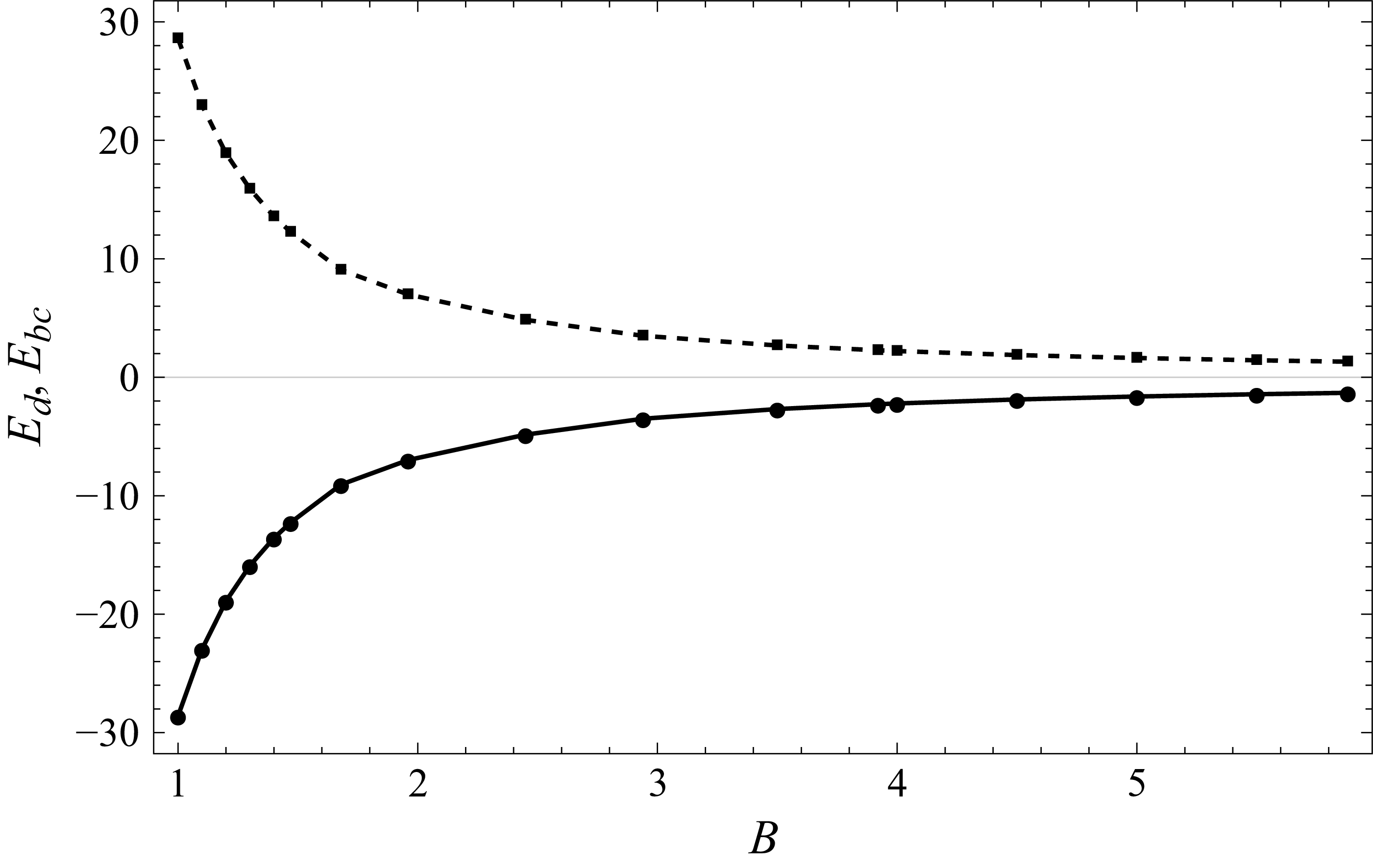
. Figure 2 shows the variations of the two contributions
 $ E_{\textit{bc}} (B)$
and
 $ E_{\textit{d}} (B)$
. It is clear that
 $ E_{\textit{d}} (B)$
is negative indicating that the viscous dissipation produces a stabilisation effect. This stabilisation is counterbalanced by a positive contribution of the solutal buoyancy
 $ E_{\textit{bc}} (B)$
acting as a source of the instability of the steady state. It is instructive to remark that
 $ |E_{\textit{d}} (B)|$
increases by reducing the aspect ratio
 $B$
, which means that the transversal confinement has a stabilisation influence at the onset of instability. Physically, the observed stabilisation is due to the additional diffusion phenomena in the
 $y$
direction induced by the transversal confinement.
Viscous dissipation contribution
 $ E_{\textit{d}}$
(solid line) and solutal buoyancy contribution
 $ E_{\textit{bc}}$
(dashed line) versus
 $B$
.

4. Numerical simulation of the three-dimensional nonlinear problem
The species transport model implemented here using the Ansys Fluent 2022 R1
 $^{\circledR }$
software is described in detail in Sanjuan et al. (Reference Sanjuan, Ali Ammar, Hirata, Ouarzazi, M. and Bou-Ali2025).
Numerical simulations are performed with four transversal aspect ratios. Two of them are chosen in a linearly stable region with
 $B=1.00$
and
 $B=1.69$
, while the others are fixed in a linearly unstable region with
 $B=3.50$
and
 $B=5.88$
. A structured hexahedral mesh of
 $75 \times 75 \times 500$
cells in the
 $x^\ast$
,
 $y^\ast$
and
 $z^\ast$
directions is used, with domain lengths
 $x^\ast = 0.51$
mm,
 $z^\ast = 30$
mm and
 $y^\ast$
ranging from
 $0.51$
to
 $3$
mm depending on the case. The corresponding spatial resolutions are
 $\Delta x^\ast = 6.8\,{\unicode{x03BC}} \mathrm{m}$
,
 $\Delta z^\ast = 60\,{\unicode{x03BC}} \mathrm{m}$
and
 $\Delta y^\ast = 6.8$
–
 $40\,{\unicode{x03BC}} \mathrm{m}$
. Mesh independence for the critical case (
 $y^\ast = 3$
mm) is verified in Sanjuan et al. (Reference Sanjuan, Ali Ammar, Hirata, Ouarzazi, M. and Bou-Ali2025), ensuring accuracy and reproducibility of the results. For the transient simulations, the maximum time-step size is set based on the maximum velocity in the
 $z$
direction, where the dominant thermogravitational convection occurs. Specifically, the time step satisfies
 $\Delta t \leqslant \Delta t_{\textit{max}} = \Delta z^\ast / w_{\textit{max}}$
for each case. This corresponds to a convective Courant–Friedrichs–Lewy condition, ensuring numerical stability. Regarding the number of iterations per time step, a convergence criterion of
 $10^{-6}$
is applied for continuity, temperature, velocity components and species.
We first simulate the transient separation of the Tol
 $|$
Ch 0.50
 $|$
0.50 mixture for different values of
 $B$
, considering
 $T_0^*$
= 298.16 K. The thermophysical properties and mass transport coefficients of that binary mixture are well documented in Lapeira et al. (Reference Lapeira, Gebhardt, Triller, Mialdun, Köhler, Shevtsova and Bou-Ali2017), and lead to
 $\psi \approx -0.05$
and
 ${\textit{Ra}}_{\textit{T}} Le=10\,000$
for
 $\Delta T^*$
= 9.833 K. For
 $\psi =-0.05$
, the linear stability analysis predicts that the transition from stable to unstable state occurs at the critical transversal aspect ratio
 $B_{\textit{c}}=2.76$
(see (3.20)).
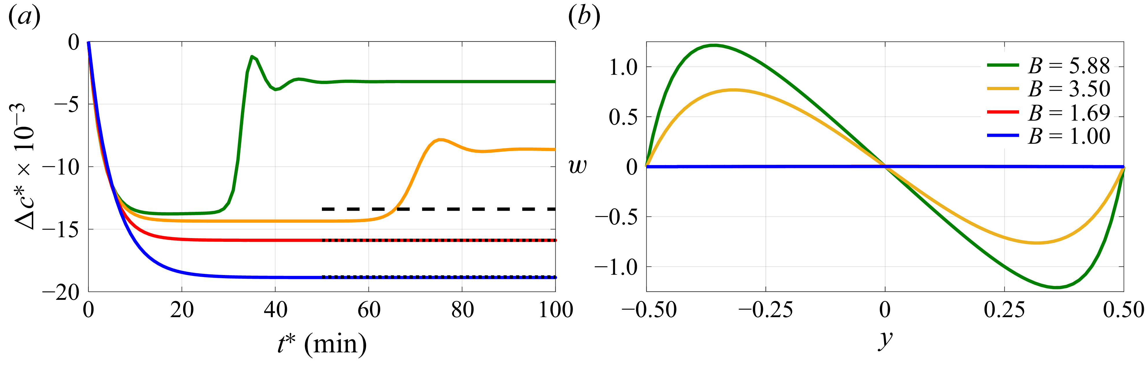
Figure 3(a) shows a negative concentration difference
 $\Delta c^*$
of the denser component between the upper and the lower limits of the cavity as a function of time. For both cases
 $B=1.00$
and
 $B=1.69$
, stable separation is reached after some time as predicted by linear stability theory. In contrast, when
 $B$
is increased to
 $3.50$
and to
 $5.88$
, the separation measured by
 $\mid \Delta c^*\mid$
in the column increases monotonically to reach a stable state over a certain period but finally becoming unstable in agreement with the linear stability analysis.
Numerical results for
 ${\textit{Ra}}_{\textit{T}}Le = 10\,000$
and
 $\psi \approx -0.05$
for different values of
 $B$
(same colour legend in both panels). (a) Time evolution of the concentration difference of the Tol component; the dashed and dotted lines indicate the steady-state separation predicted by (1.1) (two-dimensional) and (1.2) (three-dimensional), respectively. (b) Vertical velocity component as a function of
 $y$
at the mid-height of the column.

Additionally, we examine flow velocity in stable and unstable cases. According to linear stability approach, the eigenfunction
 $w_{\textit{p}}$
is given by (3.15) at the onset of instability. In this context, figure 3(b) presents the variation of the steady-state vertical velocity as a function of the horizontal coordinate
 $y$
at the centre of the column
 $x=0$
and
 $z=0$
. For unstable configurations (
 $B = 3.50$
and
 $B = 5.88$
), the odd symmetry of
 $w$
with respect to
 $y$
represents a physical signature of the descending and ascending convective currents, which enhance the mixing of the binary fluid components and disrupt the basic vertical concentration gradient. On the contrary, for both
 $B=1.69$
and
 $B=1.00$
, the vertical velocity as a function of
 $y$
is zero and the basic adverse density gradient is stable.
Numerical results: contour maps in the vertical middle planes
 $x^*=0$
and
 $y^*=0$
representing the vertical velocity component, the temperature field and the concentration of the denser species within the TGC cavity at selected time instants
 $t^*$
. (a) Unstable configuration with transverse aspect ratio
 $B = 5.88$
and (b) stable configuration with
 $B = 1.69$
.

Figure 4. Long description
Panel A: Unstable configuration with transverse aspect ratio. Three sets of contour maps are shown for different time instants (16 min, 30 min, 120 min). Each set includes vertical velocity component, temperature field, and concentration of the denser species. The vertical velocity component ranges from −4.77 to 4.76 times 10^−4 m/s, temperature ranges from 293.2 to 303.1 K, and concentration ranges from 0.4870 to 0.5129 gg^−1. The maps show changes in these parameters over time. Panel B: Stable configuration with transverse aspect ratio. Similar to Panel A, three sets of contour maps are shown for the same time instants. The vertical velocity component ranges from −3.11 to 3.13 times 10^−4 m/s, temperature ranges from 293.2 to 303.1 K, and concentration ranges from 0.4890 to 0.5110 gg^−1. The maps illustrate the distribution and evolution of these parameters over time.
In figure 4 contour maps are presented to better understand the complex spatio-temporal behaviour for the key physical quantities. Two different cases of
 $B$
are considered: the first,
 $B=5.88$
, leads to an unstable state and the second,
 $B=1.69$
, to a stable steady state. The maps show the spatial distribution of the vertical flow velocity, temperature and toluene mass fraction in dimensional form along the vertical middle planes
 $x^*=0$
and
 $y^*=0$
. Three characteristic time instants are considered. At
 $t^*$
= 16 min, the system is within the initial stability window, during which the adverse density gradient is still preserved in both configurations of
 $B$
. Thermogravitational convection is evident in the
 $x^*$
direction, driven by the applied horizontal temperature difference. We observe that for
 $B=5.88$
, early signs of convective flow begin to appear, while for
 $B=1.69$
, no such disturbances are detected. At
 $t^*$
= 30 min, the convective currents in the
 $y^*$
direction intensify for
 $B=5.88$
, leading to a progressive destabilisation of the negative mixture. This destructive flow disrupts the previously established stratification. In contrast, the system with
 $B=1.69$
remains stable, with no emergence of convection and a consistent adverse concentration gradient along the column is established. At
 $t^*$
= 120 min, the system has reached thermohydrodynamic equilibrium. For
 $B=5.88$
, the binary mixture is fully destabilised, and no concentration stratification is visible within the TGC cavity. Conversely, for
 $B=1.69$
, the cavity preserves a stable adverse density gradient, illustrating complete thermogravitational stability. Through numerical simulations, no perturbations are observed in the temperature field for either configuration, confirming that the destabilisation of the negative system is primarily driven by the onset of transverse convective flows.
Numerical characterisation of confinement-induced stabilisation. Time evolution of the normalised species separation
 $\Delta c_{\textit{Num}}^\ast / \Delta c_{\textit{FJO}}^\ast$
for different separation ratios (
 $\psi$
) at fixed transverse aspect ratio (
 $B = 1.69$
) and
 ${\textit{Ra}}_{\textit{T}}Le =10\,000$
. Mixtures with weakly negative
 $\psi$
reach a steady state, whereas larger
 $|\psi |$
leads to delayed instability. The results identify the dependence of stability on the separation ratio and support the existence of a confinement-controlled stability threshold.

Based on the numerical results obtained, it is confirmed that it is possible to stabilise the negative mixture Tol
 $|$
Ch 0.50
 $|$
0.50 (
 $\psi \approx -0.05$
) under the condition
 $B \leqslant 2.76$
, independently of the applied temperature difference, provided that the condition
 ${\textit{Ra}}_{\textit{T}}Le \geqslant ({\textit{Ra}}_{\textit{T}}Le )_{\textit{c}}(B)$
is satisfied.
In order to further investigate this behaviour, the analysis has been extended to assess the influence of the separation ratio
 $\psi$
on the thermogravitational stability of negative systems, since this parameter encapsulates the thermophysical properties and mass transport coefficients of the mixture in a dimensionless form. In this context, according to the linear stability analysis, the critical threshold of
 $\psi$
for
 $B = 1.69$
is
 $\psi _{\textit{c}} = -0.20$
. Consequently, four different values of
 $\psi$
are considered. The square symbols in figure 1(b) indicate the values of
 $\psi$
investigated numerically:
 $\psi = -0.05$
and
 $\psi = -0.10$
correspond to stable cases, whereas
 $\psi = -0.25$
and
 $\psi = -0.50$
represent unstable configurations. Within this framework, the numerical results presented in figure 5 confirm these predictions. Systems with
 $\psi = -0.05$
and
 $\psi = -0.10$
remain stable, while those with
 $\psi = -0.25$
and
 $\psi = -0.50$
exhibit instability for the configuration
 $B = 1.69$
. Moreover, it is observed that the characteristic time for the onset of instability in the case
 $\psi = -0.25$
is significantly longer than that corresponding to
 $\psi = -0.50$
. This difference can be attributed to the closer proximity of the case
 $\psi = -0.25$
to the neutral stability curve shown in figure 1(b).
The numerical analysis carried out demonstrates that the thermogravitational stability of a negative mixture strongly depends on the critical parameters
 $B$
and
 $\psi$
. As the separation ratio of the system increases, stronger transverse confinement of the cavity is required in order to suppress the onset of perturbing flows and maintain system stability. Furthermore, the numerical results show that, as
 $B$
is reduced, component separation increases, following the same behaviour observed in positive mixtures in Sanjuan et al. (Reference Sanjuan, Ali Ammar, Hirata, Ouarzazi, M. and Bou-Ali2025). This highlights the possibility of determining the thermodiffusion coefficient in negative systems using transversely confined cavities, in combination with solution (1.2).
5. Experimental validation
This section presents the experimental results obtained for the reference negative system Tol
 $|$
Ch 0.50
 $|$
0.50 with negative
 $\psi$
at
 $T_0^* = 298.16\,\textit{K}$
and under different
 ${\textit{Ra}}_{\textit{T}}Le$
conditions (
 $\psi \approx -0.05$
). First, we provide a brief summary of the experimental methodology already described in Sanjuan et al. (Reference Sanjuan, Ali Ammar, Hirata, Ouarzazi, M. and Bou-Ali2025). Thereafter, the acquired results are compared with the theoretical and numerical solutions. To further corroborate the robustness and generality of the experimental findings, the thermogravitational stability of additional negative mixtures Tol
 $|$
EtOH 0.80
 $|$
0.20 (
 $\psi \approx -0.05$
) and Tol
 $|$
MeOH 0.8420
 $|$
0.1520 (
 $\psi \approx -0.07$
) has also been examined.
5.1. Experimental methodology
Experiments were conducted using two
 $\mu$
TGCs of different transverse aspect ratios. The first
 $\mu$
TGC has dimensions
 $H = 30$
mm,
 $b = 3$
mm and
 $e = 0.51 \pm 0.025$
mm (
 $B=5.88$
), while the second one, recently installed to analyse the effect of the transverse aspect ratio
 $B$
, has dimensions
 $H = 30$
mm,
 $b = 0.98$
mm and
 $e = 0.58 \pm 0.01$
mm (
 $B=1.69$
). This selection of
 $\mu$
TGCs is motivated by the fact that the cell with
 $B = 5.88$
exhibits a higher transverse aspect ratio and, according to theoretical and numerical results, is unstable for the selected
 $|\psi |$
range
 $|\psi |\approx 0.05{-}0.07$
. The other cavity, with
 $B = 1.69$
, allows the stabilisation of an adverse density gradient, in accordance with linear stability theory. To investigate the thermogravitational behaviour of the mixture thermodiffusion experiments were conducted using optical digital interferometry, enabling real-time monitoring of species separation throughout the process. The complete methodology is documented in Sanjuan et al. (Reference Sanjuan, Ali Ammar, Hirata, Ouarzazi, M. and Bou-Ali2025).
5.2. Experimental results and comparison with linear stability and numerical solutions
We present the experimental results obtained by analysing the vertical species separation of the Tol
 $|$
Ch system in two distinct
 $\mu$
TGCs (
 $B = 5.88$
and
 $B = 1.69$
) after imposing a temperature difference. In each case, the species separation is examined for several values of
 $\Delta T^*$
, and therefore under different
 ${\textit{Ra}}_{\textit{T}} Le$
conditions, always ensuring
 ${\textit{Ra}}_{\textit{T}} Le \gt ({\textit{Ra}}_{\textit{T}}Le)_{\textit{c}} = 6225.13$
for the
 $\mu$
TGC with
 $B = 5.88$
and
 ${\textit{Ra}}_{\textit{T}}Le \gt ({\textit{Ra}}_{\textit{T}} Le)_{\textit{c}} = 7235.55$
for the
 $\mu$
TGC with
 $B = 1.69$
(see Sanjuan et al. Reference Sanjuan, Ali Ammar, Hirata, Ouarzazi, M. and Bou-Ali2025). Additionally, the experimental results are compared against the standard FJO solution (1.1), the three-dimensional theoretical model (1.2) and numerical simulations.
Figure 6(a) shows the variation of the concentration difference,
 $\Delta c^*_{\textit{Exp}}$
, for
 $B = 5.88$
as a function of time. The experimental data indicate that the solution is completely unstable, regardless of the applied temperature difference. In contrast, figure 6(b) confirms the thermogravitational stability of the component enrichments under an adverse density gradient for
 $B = 1.69$
, in agreement with predictions from linear stability theory and numerical simulations. Movies of the experimental temporal evolution of the concentration fields are provided as supplementary movies S1 (
 $B = 5.88$
) and S2 (
 $B = 1.69$
) available at https://doi.org/10.1017/jfm.2026.11755.
These results confirm that transverse confinement can fully stabilise an adverse density gradient in a negative-Soret mixture. Measurements on additional mixtures with similar and larger
 $|\psi |$
(toluene
 $|$
methanol and toluene
 $|$
ethanol) exhibited the same stabilisation behaviour for
 $B=1.69$
(see figure 7), further supporting the role of
 $\psi$
in setting the stability threshold.
Experimental evidence of confinement-induced stabilisation in a TGC. Temporal evolution of the concentration difference (
 $\Delta c^\ast _{\textit{Exp}}$
) for the Tol
 $|$
Ch 0.50
 $|$
0.50 mixture (
 $\psi \approx -0.05$
) in two microcolumns with different transverse aspect ratios. (a) Weak confinement (
 $B$
= 5.88): the system does not reach a steady-state plateau, indicating instability. (b) Stronger confinement (
 $B$
= 1.69): the system evolves towards a stable steady state with no late-time destabilisation. Insets on the right show representative interferometric concentration fields. The results demonstrate that transverse confinement suppresses the instability associated with negative Soret coefficients.

Figure 6. Long description
Panel A: A scatter plot shows the temporal evolution of the concentration difference for a mixture in a microcolumn with weak confinement. The x-axis represents time in minutes, and the y-axis represents the concentration difference. Two datasets are plotted: one with orange circles for a temperature difference of 6.6 K and another with blue squares for 8.2 K. The plot indicates that the system does not reach a steady-state plateau, suggesting instability. Insets on the right show interferometric concentration fields at specific times, with color scales indicating concentration levels. Panel B: Another scatter plot shows the temporal evolution of the concentration difference for the same mixture in a microcolumn with stronger confinement. The x-axis represents time in minutes, and the y-axis represents the concentration difference. Two datasets are plotted: one with orange circles for a temperature difference of 6.6 K and another with blue squares for 8.2 K. The plot indicates that the system evolves towards a stable steady state with no late-time destabilization. Insets on the right show interferometric concentration fields at specific times, with color scales indicating concentration levels.
Experimental temporal evolution of the concentration fields for (a) Tol
 $|$
EtOH 0.80
 $|$
0.20 and (b) Tol
 $|$
MeOH 0.8420
 $|$
0.1520 negative mixtures in the cavity with
 $B = 1.69$
. Both cases confirm stabilisation of the adverse concentration gradient under strong transverse confinement.

Steady-state vertical concentration profiles
 $c^*(z)$
of the Tol species from experiments in the Cartesian TGC (
 $B=1.69$
) for the Tol
 $|$
Ch (0.50
 $|$
0.50) mixture at different
 ${\textit{Ra}}_{\textit{T}}Le$
conditions. The linearity of profiles indicates a stable stratification along the column height.

In order to quantitatively compare the theoretical, numerical and experimental results, figure 8 shows the steady-state vertical concentration profile of the Tol component along the height of the
 $\mu$
TGC cavity for the stable case of
 $B=1.69$
and distinct
 ${\textit{Ra}}_{\textit{T}} Le$
conditions. For this comparison, the reference negative mixture (Tol
 $|$
Ch 0.50
 $|$
0.50) is selected, since the experimentally measured concentration difference is slightly larger compared with the other systems.
The profiles in figure 8 confirm that the established adverse density gradient remains stable along the height of the microcolumn and is independent of the applied temperature difference. The concentration difference
 $\Delta c^*_{\textit{Exp}}$
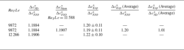
in the steady-state regime is determined from the slopes of these profiles. Table 2 then compares the experimental values with the two-dimensional FJO theory, (1.1), the three-dimensional theoretical expression, (1.2), and numerical results. A deviation greater than
 $20\,\%$
is observed for the FJO theory, whereas the maximum deviation for the three-dimensional theory does not exceed
 $2\,\%$
.


6. Conclusions
This study demonstrates that lateral confinement stabilises the adverse density gradient in a TGC. While a two-dimensional analysis (infinite layer) predicts unconditional instability, our integrated approach, combining three-dimensional linear stability theory (under the assumptions of large vertical aspect ratio
 $A \gg 1$
and stationary modes
 $k = w = 0$
), nonlinear numerical simulations and experiments, demonstrates that reducing the transverse aspect ratio
 $B$
of a parallelepipedal cavity provides a robust stabilising mechanism.
A linear stability analysis for a Cartesian TGC reveals that the critical conditions depend strongly on confinement, leading to a practical stability criterion
 $B \lt B_{\textit{c}}(\psi )$
or equivalently
 $|\psi | \lt |\psi _{\textit{c}}(B)|$
. Stability thus emerges from a competition between geometric confinement and the strength of thermodiffusive coupling, quantified by the separation ratio
 $\psi$
.
Three-dimensional nonlinear simulations performed for selected pairs (
 $\psi$
,
 $B$
) confirm these predictions. For Tol
 $|$
Ch 0.50
 $|$
0.50 with
 $\psi \approx -0.05$
, numerical simulations showed instability for
 $B=3.50$
and
 $B=5.88$
, but confirm stability for
 $B=1.69$
and
 $B= 1.00$
. Furthermore, numerical results indicated that for a prescribed value
 $B=1.69$
, the basic state is stable for
 $\psi =-0.052$
and
 $\psi =-0.10$
and unstable for
 $\psi =-0.25$
and
 $\psi =-0.50$
in agreement with linear stability results. An energy budget analysis clarifies the physical mechanisms underlying this stabilisation.
Experimental validation, based on optical interferometry in two
 $\mu$
TGCs, confirms these findings. As predicted, the analysed negative systems in the range
 $|\psi |\approx 0.05{-}0.07$
are unstable for the condition
 $B=5.88$
, while remaining stable for
 $B=1.69$
. Thus, for the first time, we demonstrate the complete stabilisation of an adverse gradient in a transversely confined Cartesian TGC, with the resulting stratification independent of the applied temperature difference
The measured steady-state concentration difference for this stable case is in excellent agreement with the three-dimensional theoretical expression (1.2). Consequently, (1.2) is validated as a reliable tool for determining the thermodiffusion coefficient
 $D_T$
from steady-state measurements in laterally confined geometries, including stabilised binary mixtures with a negative separation ratio.
Supplementary movies
Supplementary movies are available at https://doi.org/10.1017/jfm.2026.11755.
Acknowledgements
In memory of Professor. J. K. Platten, Professor. A. Zebib and Professor. J. A. Madariaga.
Funding
A.S.E. acknowledges support from the Basque Government through an FPI grant (
 $\text{PRE}\_2025\_2\_0144$
). M.M.B.-A. acknowledges financial support from the Research Group Programme (IT1902-26, Basque Government), SMART
 $\mu$
s (kk-2025/00058, Basque Government), and the projects PID2023-149539NB-C33 and PCI2024-155071-2, funded by MICINN/FEDER and MCIN/AEI, respectively (Spanish Government).
Declaration of interests
The authors report no conflict of interest.

 RaS
 RaSw
 B
 RaS,Expw≈0.296

 |ψ|
 RaTLe
 B
 |ψ|
 B
 Bc(ψ)
 B=1.00
 1.69
 3.50
 5.88
 |ψ|≈0.05
 B=1.69
 |ψ|=0.05
 0.10
 0.25
 0.50
 Ed
 Ebc
 B
 RaTLe=10000
 ψ≈−0.05
 B
 y

 x∗=0
 y∗=0
 t∗
 B=5.88
 B=1.69

 ΔcNum∗/ΔcFJO∗
 ψ
 B=1.69
 RaTLe=10000
 ψ
 |ψ|

 ΔcExp∗
 |
 |
 ψ≈−0.05
 B
 B

 |
 |
 |
 |
 B=1.69

 c∗(z)
 B=1.69
 |
 |
 RaTLe
 |
 |
 RaTLe



