2.1. Inflation can look diminished

Suppose that during each year $$j\in \{ 1,\:\,\ldots\,,\:J\} $$ for J consecutive years, we observe insurance claims that follow the folded-t distribution, which has been successfully used by Brazauskas & Kleefeld (Reference Brazauskas and Kleefeld2011, Reference Brazauskas and Kleefeld2014) and Scollnik (Reference Scollnik2014) to model insurance data. In particular, the authors have demonstrated that this distribution well captures the highly skewed and heavy-tailed nature of insurance claims. The survival function of the folded-t distribution is given by

(1) $$S_{{{\rm FT}(\nu ,\:\sigma )}} (x)=2\:S_{{{\rm T}(\nu )}} (x/\sigma ),\quad \quad x \,\gt\, 0$$

where 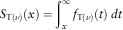$$S_{{{\rm T}(\nu )}} (x)=\mathop{\int}\nolimits_x^\infty f_{{{\rm T}(\nu )}} (t)\;dt$$ is the survival function of Student’s t distribution with $$\nu$$ degrees of freedom, and its density $$f_{{{\rm T}(\nu )}} $$ is defined by

$$f_{{{\rm T}(\nu )}} (t)={{\Gamma \left( {{{\nu {\plus}1} \over 2}} \right)} \over {\Gamma \left( {{\nu \over 2}} \right)\Gamma \left( {{1 \over 2}} \right)}}{1 \over {\sqrt \nu }}{1 \over {\left( {1{\plus}t^{2} /\nu } \right)^{{(\nu {\plus}1)/2}} }},\quad \quad {\minus}\infty \,\lt\, t \,\lt\, \infty$$

where Г denotes the gamma function. (Note that v>0 is not required to be integer.) As follows from Brazauskas & Kleefeld (Reference Brazauskas and Kleefeld2011, section 2), the mean and the median of $$X_{{{\rm FT}(\nu ,\:\sigma )}} \,\sim\,S_{{{\rm FT}(\nu ,\:\sigma )}} $$ are given by the formulas

(2) $${\rm E} \left[ {X_{{{\rm FT}(\nu ,\:\sigma )}} } \right]=\sigma \:\sqrt \nu \:{{\Gamma \left( {{{\nu {\minus}1} \over 2}} \right)} \over {\Gamma \left( {{\nu \over 2}} \right)\Gamma \left( {{1 \over 2}} \right)}},\quad \quad \nu \,\gt\, 1$$

and

(3) $${\rm median} \left[ {X_{{{\rm FT}(\nu ,\:\sigma )}} } \right]=\sigma \:F_{{{\rm T}(\nu )}}^{{{\minus}1}} (0.75)$$

where $$F_{{{\rm T}(\nu )}}^{{{\minus}1}} $$ is the quantile function of Student’s t distribution with v degrees of freedom. Now we are ready to provide our first bit of information about Figure 1.

Note 2.1. Let ν=2, σ ₀=0.93, and $$\sigma _{j} =\sigma _{0} (1{\plus}r)^{{j{\minus}1}} $$ with r=0.10. With σ _j instead of σ on the right-hand sides of equations (2) and (3), the resulting means and medians of the losses for each of the 6 years $$j=1,2,\:\,\ldots\,\:,6$$ are depicted in the top left-hand panel of Figure 1.

Furthermore, for the truncated (at d) and limited (at u) folded-t random variable, the survival function can be derived as follows:

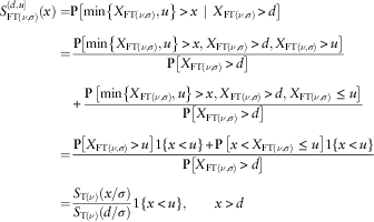(4) $$\eqalignno{ S_{{{\rm FT}(\nu ,\:\sigma )}}^{{(d,u]}} (x)= & {\bf P}\left[ {\min \left\{ {X_{{{\rm FT}(\nu ,\:\sigma )}} ,u} \right\} \,\gt\, x\,\mid\,X_{{{\rm FT}(\nu ,\:\sigma )}} \,\gt\, d} \right] \cr = & {{{\bf P}\left[ {\min \left\{ {X_{{{\rm FT}(\nu ,\:\sigma )}} ,u} \right\} \,\gt\, x,X_{{{\rm FT}(\nu ,\:\sigma )}} \,\gt\, d,\:X_{{{\rm FT}(\nu ,\:\sigma )}} \,\gt\, u} \right]} \over {{\bf P}\left[ {X_{{{\rm FT}(\nu ,\:\sigma )}} \,\gt\, d} \right]}} \cr {\plus} {{{\bf P}\,\left[ {\min \left\{ {X_{{{\rm FT}(\nu ,\:\sigma )}} ,u} \right\} \,\gt\, x,\:X_{{{\rm FT}(\nu ,\:\sigma )}} \,\gt\, d,\:X_{{{\rm FT}(\nu ,\:\sigma )}} \,\leq\, u} \right]} \over {{\bf P}\left[ {X_{{{\rm FT}(\nu ,\:\sigma )}} \,\gt\, d} \right]}} \cr = & {{{\bf P}\left[ {X_{{{\rm FT}(\nu ,\:\sigma )}} \,\gt\, u} \right]1\left\{ {x \,\lt\, u} \right\}{\plus}{\bf P}\,\left[ {x \,\lt\, X_{{{\rm FT}(\nu ,\:\sigma )}} \,\leq\, u} \right]1\left\{ {x \,\lt\, u} \right\}} \over {{\bf P}\left[ {X_{{{\rm FT}(\nu ,\:\sigma )}} \,\gt\, d} \right]}} \cr = & {{S_{{{\rm T}(\nu )}} (x/\sigma )} \over {S_{{{\rm T}(\nu )}} (d/\sigma )}}1\left\{ {x \,\lt\, u} \right\},\quad \quad x \,\gt\, d $$

where the indicator $$1\{ x \,\lt\, u\} $$ is equal to 1 when x<u and 0 when x≥u. (Note that $$S_{{{\rm FT}(\nu ,\:\sigma )}}^{{(d,u]}} (x)=1$$ for x≤d.) To derive formula for the mean of the truncated-and-limited folded-t random variable $$X_{{{\rm FT}(\nu ,\:\sigma )}}^{{(d,u]}} \,\sim\,S_{{{\rm FT}(\nu ,\:\sigma )}}^{{(d,u]}} $$ , we use expression (4), integration by parts, and straightforward simplifications:

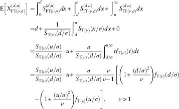(5) $$\eqalignno{ {\bf E}\left[ {X_{{{\rm FT}(\nu ,\:\sigma )}}^{{(d,u]}} } \right]= &#x0026; \mathop{\int}\nolimits_0^d S_{{{\rm FT}(\nu ,\sigma )}}^{{(d,u]}} dx{\plus}\mathop{\int}\nolimits_d^u S_{{{\rm FT}(\nu ,\sigma )}}^{{(d,u]}} dx{\plus}\mathop{\int}\nolimits_u^\infty S_{{{\rm FT}(\nu ,\sigma )}}^{{(d,u]}} dx \cr = &#x0026; d {\plus} {1 \over {S_{{{\rm T}(\nu )}} (d/\sigma )}}\mathop{\int}\nolimits_d^u S_{{{\rm T}(\nu )}} (x/\sigma )dx{\plus}0 \cr = &#x0026; {{S_{{{\rm T}(\nu )}} (u/\sigma )} \over {S_{{{\rm T}(\nu )}} (d/\sigma )}} \cdot u {\plus} {\sigma \over {S_{{{\rm T}(\nu )}} (d/\sigma )}}\mathop{\int}\nolimits_{d/\sigma }^{u/\sigma } tf_{{{\rm T}(\nu )}} (t)dt \cr = &#x0026; {{S_{{{\rm T}(\nu )}} (u/\sigma )} \over {S_{{{\rm T}(\nu )}} (d/\sigma )}} \cdot u {\plus} {\sigma \over {S_{{{\rm T}(\nu )}} (d/\sigma )}}{\nu \over {\nu {\minus}1}}\left[ {\left( {1{\plus}{{(d/\sigma )^{2} } \over \nu }} \right)f_{{{\rm T}(\nu )}} (d/\sigma )} \right. \cr {\minus} \left( {1{\plus}{{(u/\sigma )^{2} } \over \nu }} \right)f_{{{\rm T}(\nu )}} (u/\sigma )\right\Bigg],\quad \quad \nu \,\gt\, 1 $$

And expression for the median of the truncated-and-limited folded-t random variable $$X_{{{\rm FT}(\nu ,\sigma )}}^{{(d,u]}} \,\sim\,S_{{{\rm FT}(\nu ,\sigma )}}^{{(d,u]}} $$ follows directly from (4):

(6) $${\rm median}\left[ {X_{{{\rm FT}(\nu ,\sigma )}}^{{(d,u]}} } \right]=\min \left\{ {u,\sigma F_{{{\rm T}(\nu )}}^{{{\minus}1}} \left( {0.5{\plus}0.5F_{{{\rm T}(\nu )}} (d/\sigma )} \right)} \right\}$$

In particular, when $$u=\infty$$ , then we call $$X_{{{\rm FT}(\nu ,\sigma )}}^{{(d,\infty]}} $$ and $$S_{{{\rm FT}(\nu ,\sigma )}}^{{(d,\infty]}} $$ the truncated (at d) folded-t random variable and survival function, respectively. The corresponding cumulative distribution function (cdf) $$F_{{{\rm FT}(\nu ,\sigma )}}^{{(d,\infty]}} $$ for various parameter values is depicted in Figure 3.

Figure 3

Complete-but-unobservable (left-hand panel) and truncated-and-observable (right-hand panel) folded-t distributions of inflated losses with v=1.5 and various values of σ.

The mean and the median of $$X_{{{\rm FT}(\nu ,\sigma )}}^{{(d,\infty]}} $$ can be derived from equations (5) and (6) by simply setting the parameter u to ∞, in which case we obtain the following equations:

(7) $$E\left[ {X_{{{\rm FT}(\nu ,\sigma )}}^{{(d,\infty]}} } \right]=\sigma {\nu \over {\nu {\minus}1}}\left( {1{\plus}{{(d/\sigma )^{2} } \over \nu }} \right)h_{{{\rm T}(\nu )}} (d/\sigma ),\quad \quad \nu \,\gt\, 1$$

and

(8) $${\rm median}\left[ {X_{{{\rm FT}(\nu ,\sigma )}}^{{(d,\infty]}} } \right]=\sigma F_{{{\rm T}(\nu )}}^{{{\minus}1}} \left( {0.5{\plus}0.5F_{{{\rm T}(\nu )}} (d/\sigma )} \right)$$

where $$h_{{{\rm T}(\nu )}} =f_{{{\rm T}(\nu )}} /S_{{{\rm T}(\nu )}} $$ denotes the hazard rate function of Student’s t distribution with v degrees of freedom. Notice also that if we let d=0 in equations (7) and (8), they become (2) and (3), respectively.

Note 2.2. Let ν=2, σ ₀=0.93, and $$\sigma _{j} =\sigma _{0} (1{\plus}r)^{{j{\minus}1}} $$ with r=0.10. Furthermore, let d=4. Then with σ _j instead of σ on the right-hand sides of equations (7) and (8), the means and the medians of the truncated (at d) losses for each of the 6 years $$j=1,2,\,\ldots\,,6$$ are depicted in the top right-hand panel of Figure 1, with the inflation rates being 0.76% (mean based) and 0.58% (median based).

2.2. Inflation can become invisible

Suppose that during each year $$j\in \{ 1,\:\,\ldots\,\:,J\} $$ for J consecutive years, we observe insurance claims that follow the classical Pareto distribution of the first kind, also known as a single-parameter Pareto distribution in actuarial literature, which has the survival function

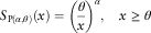(9) $$S_{{{\rm P}(\alpha ,\theta )}} (x)=\left( {{\theta \over x}} \right)^{\alpha } ,\quad x\,\geq\, \theta $$

where α>0 and θ>0 are the shape and scale parameters, respectively. Recall that the mean of this distribution is $$\alpha \theta /(\alpha {\minus}1)$$ , assuming of course $$\alpha \,\gt\, 1$$ , and the median is $$2^{{1/\alpha }} \theta $$ .

Note 2.3. Let α=2, θ ₀=0.66, and $$\theta _{j} =\theta _{0} (1{\plus}r)^{{j{\minus}1}} $$ with r=0.10. With θ _j instead of θ, the resulting means and medians of the losses for each of the 6 years $$j=1,2,\:\,\ldots\,\:,6$$ are depicted in the middle left-hand panel of Figure 1.

Furthermore, the truncated (at d) and limited (at u) Pareto random variable has the survival function (cf. equation (4)):

$$S_{{{\rm P}(\alpha ,\theta )}}^{{(d,u]}} (x)=\left( {{d \over x}} \right)^{\alpha } 1\{ x \,\lt\, u\} ,\quad \quad x \,\gt\, d$$

Hence, the corresponding mean and median are

(10) $${\bf E}\left[ {X_{{{\rm P}(\alpha ,\theta )}}^{{(d,u]}} } \right]={{\alpha d} \over {\alpha {\minus}1}}{\minus}{{u(d/u)^{\alpha } } \over {\alpha {\minus}1}},\quad \alpha \,\gt\, 1$$

and

(11) $${\rm median}\left[ {X_{{{\rm P}(\alpha ,\theta )}}^{{(d,u]}} } \right]=\min \left\{ {u,2^{{1/\alpha }} d} \right\}$$

Also, when $$u=\infty$$ , then we call $${X_{{{\rm P}(\alpha ,\theta )}}^{{(d,\infty]}} }$$ and $$S_{{{\rm P}(\alpha ,\theta )}}^{{(d,\infty]}}$$ the truncated (at d) Pareto random variable and survival function, respectively. The corresponding cdf $$F_{{{\rm P}(\alpha ,\theta )}}^{{(d,\infty]}}$$ for various parameter values is depicted in Figure 4.

Note 2.4. Let α=2, θ ₀=0.66, and $$\theta _{j} =\theta _{0} (1{\plus}r)^{{j{\minus}1}} $$ with r=0.10. Furthermore, let d=4 and $$u=\infty$$ . As equations (10) and (11) are independent of θ _j’s, we have constant means and medians of the truncated (at d) losses for each of the 6 years $$j=1,2,\:\,\ldots\,\:,6$$ . This fact is seen from the middle right-hand panel of Figure 1, where the inflation rate is 0%.

Figure 4

Complete-but-unobservable (left-hand panel) and truncated-and-observable (right-hand panel) Pareto distributions of inflated losses with $$\alpha =0.5$$ and various θ.

2.3. Inflation can look even like deflation

Suppose that during each year $$j\in \{ 1,\,\ldots\,\:,J\} $$ for J consecutive years, we observe insurance claims that follow what we call the polynomial Pareto (PP) distribution, which has the survival function

(12) $$S_{{{\rm PP}(\alpha ,\beta ,\theta )}} (x)=\left( {{\theta \over x}} \right)^{\alpha } \exp \left\{ {\beta \left( {{1 \over x}{\minus}{1 \over \theta }} \right)} \right\},\quad x\,\geq\, \theta $$

with parameters $$\alpha \,\gt\, 0$$ , $$\beta \,\geq\, 0$$ , and $$\theta \,\gt\, 0$$ . Notice that when $$\beta =0$$ , then formula (12) reduces to (9) and thus the PP model becomes the standard Pareto one. We note in passing that we have created the PP distribution specifically for the purpose of illustrating the message stated in the title of this subsection. For other similar distributions, we refer to, for example, Lai & Xie (Reference Lai and Xie2006) and Marshall & Olkin (Reference Marshall and Olkin2007).

Figure 5

Complete-but-unobservable (left-hand panel) and truncated-and-observable (right-hand panel) polynomial Pareto distributions of inflated losses with $$\alpha =0.5$$ and various values of β and θ.

Note 2.5. The hazard rate function of the PP distribution is

$$h_{{{\rm PP}(\alpha ,\beta ,\theta )}} (x)={\alpha \over x}{\plus}{\beta \over {x^{2} }},\quad x\,\geq\, \theta $$

which can be viewed as a polynomial of the standard Pareto hazard rate function 1/x, and this explains why we have decided to call this distribution “polynomial Pareto”. Note also that h _PP is a special case of the class of rational hazard rate functions (cf. e.g. Bebbington et al., Reference Bebbington, Lai, Murthy and Zitikis2011a).

Similar to the previous subsection, the truncated (at d) and limited (at u) PP random variable has the survival function

$$S_{{{\rm PP}(\alpha ,\beta ,\theta )}}^{{(d,u]}} (x)=\left( {{d \over x}} \right)^{\alpha } \exp \left\{ {\beta \left( {{1 \over x}{\minus}{1 \over d}} \right)} \right\}1\{ x \,\lt\, u\} ,\quad \quad x \,\gt\, d$$

Unlike in the previous sections, the mean and the median of this distribution cannot be reduced to simple closed-form expressions, and thus we have to evaluate them numerically.

In addition, when $$u=\infty$$ , then we call $$X_{{{\rm PP}(\alpha, \beta, \theta )}}^{{(d,\infty]}} $$ and $$S_{{{\rm PP}(\alpha, \beta, \theta)}}^{{(d,\infty]}} $$ the truncated (at d) polynomial Pareto random variable and survival function, respectively. The corresponding cdf $$F_{{{\rm PP}(\alpha ,\beta, \theta)}}^{{(d,\infty]}} $$ for various parameter values is depicted in Figure 5. Now we are ready to present our last bit of information about Figure 1.

Note 2.6. Let α=β=2, θ ₀=1, $$\beta _{j} =\beta _{0} (1{\plus}r)^{{j{\minus}1}} $$ and $$\theta _{j} =\theta _{0} (1{\plus}r)^{{j{\minus}1}} $$ with r=0.10. The means and the medians of the ground-up losses for each of the 6 years $$j=1,2,\:\,\ldots\,\:,6$$ are depicted in the bottom left-hand panel of Figure 1. Furthermore, with d=4 and $$u=\infty$$ , the means and the medians of the truncated (at d) losses for each of the 6 years $$j=1,2,\:\,\ldots\,\:,6$$ are depicted in the bottom right-hand panel of Figure 1, with the inflation rates being −1.05% (mean based) and −0.53% (median based).

3.1. Model

Suppose that during each year $$j\in \{ 1,\:\,\ldots\,\:,J\} $$ for J consecutive years, random variables $$Y_{{j,1}} ,\:\,\ldots\,\:,Y_{{j,N_{j} }} $$ manifest themselves but not all of them are actually seen. Namely, we can see only those $$Y_{{j,k}} $$ ’s whose values are in a certain layer, say in the interval $$(d_{j} ,u_{j} ]$$ ; we can think of the lower limit d _j as an insurance deductible and of the upper limit u _j as an insurance policy limit. Hence, we observe the random variables:

$$X_{{j,k}} =\min \{ Y_{{j,k}} ,u_{j} \} \,\mid\,Y_{{j,k}} \,\gt\, d_{j} $$

and there are $$M_{j} =\mathop{\sum}\nolimits_{i=1}^{N_{j} } 1\{ Y_{{j,k}} \,\gt\, d_{j} \} $$ of them with values either $$Y_{{j,k}} $$ or u _j depending on the magnitude of $$Y_{{j,k}} $$ .

Denote the distribution of the counts N _j by $${\cal P}_{j} =\{ P_{j} (n),n=0,1,2,\,\ldots\,\} $$ . These integer-valued random variables N _j are not observable; only M _j’s are observable. Denote the distribution of M _j by $${\cal Q}_{j} =\{ Q_{j} (m),m=0,1,2,\,\ldots\,\} $$ , which is given by the formula

$$Q_{j} (m)=\mathop{\sum}\limits_{n=m}^\infty P_{j} (n)\left( {\matrix{ n \cr m \cr } } \right)S_{j}^{m} (d_{j} )F_{j}^{{n{\minus}m}} (d_{j} )$$

The following examples (cf. e.g. Klugman et al., Reference Klugman, Panjer and Willmot2008) illustrate the distributions $${\cal P}_{j} $$ and $${\cal Q}_{j} $$ :

1. E1. If $$P_{j} (n)={\rm Poisson}(n\,\mid\,\lambda _{j} )$$ for all $$n=0,1,2,\,\ldots\,$$ , where $$\lambda _{j} \,\gt\, 0$$ is a parameter, then $$Q_{j} (m)={\rm Poisson}(n\,\mid\,\lambda _{j} S_{j} (d_{j} ))$$ for all $$m=0,1,2,\,\ldots\,$$ .

2. E2. If $$P_{j} (n)={\rm NB}(n\,\mid\,\alpha _{j} ,\theta _{j} )$$ for all $$n=0,1,2,\,\ldots\,$$ , where $$\alpha _{j} \,\gt\, 0$$ and $$\theta _{j} \,\gt\, 0$$ are parameters, and NB stands for the negative binomial distribution, then $$Q_{j} (m)={\rm NB}(n\,\mid\,\alpha _{j} ,\theta _{j} S_{j} (d_{j} ))$$ for all $$m=0,1,2,\,\ldots\,$$ .

3. E3. If $$P_{j} (n)=\mathop{\int} {\rm Poisson}(n\,\mid\,\lambda )dG_{j} (\lambda )$$ for all $$n=0,1,2,\,\ldots\,$$ , where $$G_{j} $$ is the cdf of a random variable, then $$Q_{j} (m)=\mathop{\int} {\rm Poisson}(n\,\mid\,\lambda S_{j} (d_{j} ))dG_{j} (\lambda )$$ for all $$m=0,1,2,\,\ldots\,$$ .

Note 3.1. When G _j is degenerate at the point $$\lambda _{j} \,\gt\, 0$$ , then (E3) reduces to (E1), and when G _j is the gamma distribution with parameters $$\alpha _{j} \,\gt\, 0$$ and $$\theta _{j} \,\gt\, 0$$ , then (E3) reduces to (E2).

Assume that all the underlying random variables $$Y_{{j,k}} $$ are independent, have densities, and let, for each year $$j\in \{ 1,\:\,\ldots\,\:,J\} $$ , the densities of the random variables $$Y_{{j,1}} ,Y_{{j,2}} ,\,\ldots\,$$ be f _j. The dependence of the density f _j on j stems from the underlying problem. Namely, we assume that there is a certain trend $$\vec {\sigma }=(\sigma _{1} ,\:\,\ldots\,\:,\sigma _{J} )$$ from year to year (think of inflation) and thus there is an underlying cdf F ₀ such that the cdf of Y _j,k is equal to $$F_{0} (y/\sigma _{j} )$$ , and thus

$$f_{j} (y)={1 \over {\sigma _{j} }}f_{0} \left( {{y \over {\sigma _{j} }}} \right)$$

where f ₀ is the density of F ₀. We also assume that $$Y_{{j,1}} ,Y_{{j,2}} ,\,\ldots\,$$ are independent of N _j, that is, the claim severities are independent of the frequencies. This is a common assumption in the classical actuarial literature (cf. e.g. Klugman et al., Reference Klugman, Panjer and Willmot2008), but there are of course many research papers that depart from it (cf. e.g. Sendova & Zitikis, Reference Sendova and Zitikis2012; Li & Sendova, Reference Li and Sendova2014; and references therein). Our task is to estimate the trend $$\vec {\sigma }$$ , keeping in mind that we observe only $$X_{{j,k}} $$ ’s, but not $$Y_{{j,k}} $$ ’s.

3.2. Estimation

To estimate the trend $$\vec {\sigma }=(\sigma _{1} ,\,\ldots\,,\sigma _{J} )$$ , we use the maximum likelihood technique and thus need to derive the complete likelihood, which is

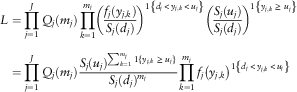(13) $$\eqalignno{ L &#x0026; =\prod\limits_{j=1}^J Q_{j} (m_{j} )\prod\limits_{k=1}^{m_{j} } \left( {{{f_{j} (y_{{j,k}} )} \over {S_{j} (d_{j} )}}} \right)^{{1\left\{ {d_{j} \,\lt\, y_{{j,k}} \,\lt\, u_{j} } \right\}}} \left( {{{S_{j} (u_{j} )} \over {S_{j} (d_{j} )}}} \right)^{{1\left\{ {y_{{j,k}} \,\geq\, u_{j} } \right\}}} \cr &#x0026; =\prod\limits_{j=1}^J Q_{j} (m_{j} ){{S_{j} (u_{j} )^{\mathop{\sum}\nolimits_{k=1}^{m_{j} } {1\{ y_{{j,k}} \,\geq\, u_{j} \} } }} \over {S_{j} (d_{j} )^{{m_{j} }} }}\prod\limits_{k=1}^{m_{j} } f_{j} \left( {y_{{j,k}} } \right)^{{1\left\{ {d_{j} \,\lt\, y_{{j,k}} \,\lt\, u_{j} } \right\}}} $$

where $$S_{j} (y)=1{\minus}F_{j} (y)$$ and m _j is the number of observed $$y_{{j,k}} $$ ’s, that is, all of those $$y_{{j,k}} $$ ’s are above d _j.

While the second equation of (13) is a simple rearrangement of the terms in the previous expression, the first equation needs some explanation. We begin by noting that, conditionally, on the number M _j=m _j of observations, the inside product on the right-hand side of the first equation multiplies the likelihoods of all the observed values: if a value $$y_{{j,k}} $$ has been recorded, then its conditional on being above d _j likelihood is $$f(y_{{j,k}} )/S_{j} (d_{j} )$$ , but if the value u _j has been recorded, then we do not know the actual value of the corresponding loss y _j,k, except that it is somewhere on or above u _j, and thus the conditional likelihood becomes $$S_{j} (u_{j} )/S_{j} (d_{j} )$$ . As the entire inside product is the conditional likelihood upon $$M_{j} =m_{j} $$ , we turn it into an unconditional likelihood by multiplying it by the probability $$Q_{j} (m_{j} )$$ of $$M_{j} =m_{j} $$ . As the losses over the J years are independent by assumption, we obtain the complete likelihood by multiplying the individual $$j=1,\:\,\ldots\,\:,J$$ likelihoods. This leads us to the complete likelihood given by formula (13).

As we observe the random variables $$X_{{j,k}} =\min \{ Y_{{j,k}} ,u_{j} \} \,\mid\,Y_{{j,k}} \,\gt\, d_{j} $$ , we next rewrite formula (13) in terms of $$x_{{j,k}} $$ ’s:

(14) $$L=\prod\limits_{j=1}^J Q_{j} (m_{j} ){{S_{j} (u_{j} )^{{\mathop{\sum}\nolimits_{k=1}^{m_{j} } {{\bf 1}\{ x_{{j,k}} =u_{j} \} } }} } \over {S_{j} \left( {d_{j} } \right)^{{m_{j} }} }}\prod\limits_{k=1}^{m_{j} } f_{j} \left( {x_{{j,k}} } \right)^{{{\bf 1}\{ x_{{j,k}} \,\lt\, u_{j} \} }} $$

We shall use formula (14) in our illustrative example below.

3.3. Example

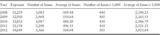
We illustrate the above ideas by considering losses of an employee group under a prescription drug coverage. Specifically, we investigate losses during the 5 consecutive years 2008–2012 for drugs prescribed to treat cancer. The data set is confidential, and we thus do not elaborate here on its source, nor provide further details, except that we do provide the necessary summary statistics that are sufficient for our following analysis and also for the appreciation of results.

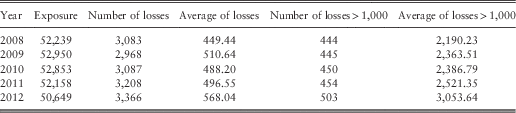
We proceed as follows. Even though our data set is complete, and we do use it to check the accuracy of our findings based on the above-described methodology, we start our considerations by first constructing a new data set by artificially imposing a deductible of 1,000 dollars on the original data. Table 1 provides summaries of the complete as well as of the truncated data that result from imposing the noted deductible. We see that there are roughly 50,000 life-years of exposure in each calendar year, meaning that ∼50,000 individuals are covered by the prescription drug insurance coverage. While the number of cancer drug losses seems high, we must recognise that a given individual may have multiple prescription drug losses in a year. Notice that a fairly small fraction of losses exceed 1,000, and that the average loss among losses above 1,000 is large owing to the long tail of the loss distribution.

Table 1

Summary of cancer drug loss data.

Histograms of the losses in each calendar year are given in the five panels of Figure 6, where we have found that it is more informative to examine histograms of the logarithms (base 10) of the losses than the histograms of the losses themselves. The distributions of the losses in excess of 1,000 are then delineated by the bars of the histograms that correspond to values greater than 3.

Figure 6

Histograms of the logarithms (base 10) of cancer drug losses for the 5 years from 2008 to 2012.

While the histograms provide information about the loss distributions, it is difficult to glean any information about the trend in loss amounts. We can calculate crude estimates of the inflation rate using the averages shown in Table 1 by the formula

$$\widehat{r}_{{{\rm crude}}} =\left( {{{{\rm average}\;{\rm loss}\;{\rm in}\;2012} \over {{\rm average}\;{\rm loss}\;{\rm in}\;2008}}} \right)^{{1/4}} {\minus}1$$

Using the averages of all loss amounts, the crude inflation rate estimate is 0.0450, but if we assume that we observe only the losses above 1,000, then the crude inflation rate estimate becomes 0.0757. We know, however, that this estimate is not an appropriate estimate because it does not correctly allow for the truncation.

In order to improve upon our estimate while still using only the observed losses that exceed 1,000, we employ the model developed above. Namely, we assume that in each year $$j=2008,\:\,\ldots\,\:,2012$$ , the number of losses follows the Poisson distribution with the mean $$\lambda _{j} =\lambda e_{j} $$ , where e _j is the exposure in the year j (see Table 1). Then the number of losses above 1,000 in the year j has a Poisson distribution with the mean $$\lambda _{j} S_{j} (1,000)$$ . We further assume that losses in each year j are independent and identically distributed, and follow the folded-t distribution with parameters v and $$\sigma _{j} =\sigma (1{\plus}r)^{{j{\minus}2008}} $$ . We have four parameters to estimate: λ, r, $$\nu$$ , and $$\sigma$$ . 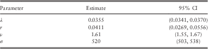Using the likelihood technique described above, we obtain the estimates reported in Table 2. A few comments follow.

Table 2

Maximum likelihood estimates of parameters with approximately 95% likelihood ratio confidence intervals.

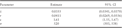
First, note that the model-based estimate 0.0411 of the true inflation rate is close to the “true” crudely estimated rate 0.0450, which is based on the entire data set. Note also that the other crude estimate 0.0757, which is based on the truncated data, is quite different from the model-based estimate.

Of course, we should bear in mind that estimates depend on how well our model describes the loss distribution for each year. We can check this for losses above 1,000. Having said this, we want to point out that given the complete data set that we actually have, we do know the loss amounts even below 1,000, but in general, we would not normally have any information about the losses below the deductible. Hence, our conclusions about loss trends would depend on some aspects of the model that may not be verifiable.

Next, our data on losses above 1,000 provide information about the product $$\lambda S_{j} (1,000)$$ , but not about λ and $$S_{j} (1,000)$$ individually. Hence, our estimates of λ and $$S_{j} (1,000)$$ may be quite poor even if our estimates of the rate at which losses above 1,000 occur and of the conditional distribution of losses above 1,000 happen to be quite good.

Finally, it would appear at least in our real-life illustrative example that having data for 5 years is not enough to obtain a very good estimate of the trend: the year-to-year variation in the loss distribution is too great. Nevertheless, the illustrative example has successfully demonstrated that with good care of the matter, one can, nevertheless, extract a reasonably accurate estimate of the true inflation rate even from data layers, such as that above deductible.