1. Introduction
Mixing is the blending of parcels of fluid that initially have different properties. Although the blending of properties relies on molecular diffusion, mixing is often collocated with occurrences of turbulence in the flow. Turbulent mixing is a two-step process comprised of stirring and diffusion (Aref Reference Aref1984; Jones Reference Jones1991). Turbulent eddies stir the fluid, sharpening density gradients and increasing the surface area over which molecular diffusion can act, leading to a more rapid blending of fluid parcels than could be achieved by laminar diffusion alone. Molecular diffusion makes mixing an irreversible process, and the change in the probability density function (p.d.f.) of the quantity being mixed allows us to identify that diffusion has occurred (Tseng & Ferziger Reference Tseng and Ferziger2001). This change in the p.d.f. is a useful and general definition of mixing. Mixing can also be characterised by various statistics linked to the change in p.d.f., e.g. the reduction in the variance of the scalar field. We focus in this paper on the use of mixing efficiency to characterise the energetics of mixing in a density stratified fluid.
Turbulent mixing involves kinetic energy to do the stirring and internal energy to drive diffusion. In the simplest case of a passive scalar, the amount of kinetic energy dissipated during a mixing event may be distinct from (or at least not closely related to) the amount of mixing achieved. The energetics of mixing in a density stratified fluid are inherently different as the change in the p.d.f. has an important impact on the potential energy of the system. The notion of ‘mixing efficiency’ seeks to understand and quantify the relationship between mixing – a change in the p.d.f. – and the energetics. It is important to recognise that the mechanical energy of the system does not define the mixing, although the energetics can impose constraints upon it.
Mixing efficiency is a commonly used parameter in models of stratified mixing in turbulent flows and the oceans (e.g. Wunsch & Ferrari Reference Wunsch and Ferrari2004). This parameter aims to quantify the fraction of energy feeding a turbulent event that is consumed by irreversible diabatic mixing, as opposed to being dissipated viscously (Winters et al. Reference Winters, Lombard, Riley and D’Asaro1995; Tailleux Reference Tailleux2009). Currently there are numerous measures of mixing efficiency, including volumetric, bulk, instantaneous and point-wise definitions, and it is often unclear how these measures are related (see Peltier & Caulfield Reference Peltier and Caulfield2003; Tailleux Reference Tailleux2009). We concentrate in this paper on a conceptually simple and widely used volumetric measure of mixing efficiency.
We may consider there to be two types of energy sources for turbulent mixing: the limiting cases corresponding to mechanically and buoyancy-driven mixing. In mechanically driven mixing, a source of kinetic energy unrelated to the stratification directly feeds the turbulence. For buoyancy-driven mixing, buoyancy forces provide the source for kinetic energy that leads to the generation of turbulence. The majority of previous work has concentrated on mechanically driven mixing, but many processes have some combination of the two energy sources and therefore measures of mixing and efficiency should be general enough to apply for either energy source (or some combination of the two).
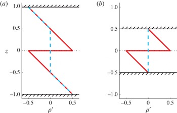
Gravitationally unstable flows (for which mixing is primarily buoyancy-driven) are often found in nature. Examples include hydrothermal plumes and radiative cooling of the ocean surface. The density profile shown in figure 1(a) can occur instantaneously during the breaking of an internal wave. Although many flows have some component of kinetic energy and will not be solely driven by buoyancy, in this paper we will make use of examples where the initial kinetic energy is zero, to illustrate specific characteristics of the mixing efficiency.
In order to avoid confusion over the various measures of mixing in a flow, we first define the mixing efficiency (§ 2.1). We compare this definition with some other commonly used measures of mixing efficiency (§ 2.2). We then demonstrate how mixing efficiency parameterisations have unexpected physical properties that require careful interpretation. These are introduced using the two examples in figure 1. Plotted are the initial and final density profiles for two initially gravitationally unstable systems. For the case where the examples begin and end with no kinetic energy, we find they have different mixing efficiencies, despite having mixing that is physically identical (i.e. the changes in the volume of each density class are the same) and identical cumulative dissipation of kinetic energy (which must be equal to the change in gravitational potential energy). The flows are effectively indistinguishable (apart from the location of the boundaries which do not play a significant role in the dynamics), but the example shown in figure 1(a) has a mixing efficiency of
 $3/4$
, whereas the example shown in figure 1(b) has a mixing efficiency of
 $2/3$
. The point is that these two flows are identical from a mixing perspective but completely different from a mixing efficiency standpoint.
Initial density profile (solid) and final density profile (dashed) for two example flows, with the same density profile in the mixing region but in differently sized tanks (hatched lines represent the upper and lower boundaries of the tank). These examples have identical mixing (identical changes in the volume of each density class), identical dissipation (net change in gravitational potential energy) but different values of mixing efficiency: (a)
 ${\it\eta}=3/4$
, (b)
 ${\it\eta}=2/3$
. Note that if there are no-flux boundary conditions there will be thin diffusion boundary layers at the top and bottom tank walls. The importance of these will depend on the ratio of the vertical to diffusion length scales.

The irreversibility of mixing occurs at the smallest scales of the flow where molecular diffusion of mass, driven by internal energy, acts to homogenise density differences. Hence, it might be expected that mixing efficiency would be independent of the large-scale turbulent flow structures at sufficiently high Reynolds number and thus dependent only upon external properties of the fluid or flow, such as the Schmidt or Richardson number (see for example Fernando Reference Fernando1991; Peltier & Caulfield Reference Peltier and Caulfield2003). This often leads to the assumption that a constant mixing efficiency is suitable for many flows if these parameters remain constant (a value often used is 0.17; Wunsch & Ferrari Reference Wunsch and Ferrari2004).
Although there has been much recent research challenging the assumption of a constant mixing efficiency (e.g. Hult, Troy & Koseff Reference Hult, Troy and Koseff2011b ; Dunckley et al. Reference Dunckley, Koseff, Steinbuck, Monismith and Genin2012; Bluteau, Jones & Ivey Reference Bluteau, Jones and Ivey2013; Lozovatsky & Fernando Reference Lozovatsky and Fernando2013; Mashayek, Caulfield & Peltier Reference Mashayek, Caulfield and Peltier2013, among others) these studies have concentrated on parameterisations of mixing using the Froude and turbulent Reynolds number in stably stratified flows, which in general have low mixing efficiencies. Higher mixing efficiencies have been found in convectively unstable stratified flows, with values of up to 0.75 measured in experiments on stratified Rayleigh–Taylor instability (Lawrie & Dalziel Reference Lawrie and Dalziel2011a ; Davies Wykes & Dalziel Reference Davies Wykes and Dalziel2014) and values approaching 1 in simulations and experiments on horizontal convection (Scotti & White Reference Scotti and White2011; Gayen et al. Reference Gayen, Griffiths, Hughes and Saenz2013). The current work emerged from a desire to understand how such high mixing efficiencies can be achieved.
As we will demonstrate in § 3.1, flows exist for which mixing efficiency depends on the density profile in regions where no motion occurs. We go on to show in § 3.2 that this effect involves ‘relabelling’ of available potential energy as background potential energy in those regions where there is no enhancement of background diffusion. In § 4, we show that this relabelling can result in a wide range of mixing efficiencies. The implications for interpretation of mixing efficiency are discussed in § 5.
2. Mixing and mixing efficiency
Consider a three-dimensional density field
 ${\it\rho}(x,y,z)$
, where
 $x$
and
 $y$
are the horizontal coordinates and
 $z$
the vertical position. Mixing of this density field will correspond to a change in the p.d.f. of density,
 ${\it\Psi}({\it\rho})$
(see Tseng & Ferziger Reference Tseng and Ferziger2001, for a definition). The p.d.f. of density for a given volume represents the fraction of that volume taken up by a particular value of density (i.e. how much of that density we have in our volume). In a closed system, the p.d.f. must change when mass diffusion occurs (as this will change how much of each density we have in our volume) and any changes in the p.d.f. must correspond directly with diffusion between fluid parcels.
Mixing is the blending of fluid parcels by diffusion, a process that is enhanced by the action of turbulence, which steepens scalar gradients and increases the isoscalar surface area over which diffusion occurs (Winters & D’Asaro Reference Winters and D’Asaro1996). It should be noted that mixing defined in this way is local: it can be defined unambiguously for a sub-volume, whereas (as we shall see shortly) both the energetic consequences of mixing and therefore mixing efficiency are global quantities that do not reflect whether mixing is localised or not. We will use the phrase ‘mixing region’ to refer to the region of the flow where turbulence is physically present, resulting in a change in the amounts of each density present in that region. For the density profiles we will consider here, the mixing region can be identified as the constant-density region in the final density profile where the density has changed from the initial conditions.
The definitions of the energetics of stratified mixing that follow are not necessarily direct measures of the homogenisation of passive scalars (e.g. nutrients, phytoplankton) unless their spatial distribution is identical to that of
 ${\it\rho}$
. There is no change in the potential energy of a system when a passive scalar is homogenised in a volume, which is not the case for mixing of a stable stratification.
2.1. Background and available potential energy
For an initially stable density profile, mixing of density raises the centre of mass of the volume and thus requires a source of energy. However, not all instantaneous increases in the centre of mass of the system are due to mixing. For a general volume, we need a method for separating changes in the potential energy due to irreversible molecular diffusion from those due to reversible processes. Following Winters et al. (Reference Winters, Lombard, Riley and D’Asaro1995), we start with gravitational potential energy in the flow, integrated over the volume
 $V$
and with gravitational acceleration
 $g$
,
 $$\begin{eqnarray}E_{p}=g\int _{V}z{\it\rho}\,\text{d}V,\end{eqnarray}$$
and partition
 $E_{p}$
into background potential energy and that which is available to do work.
For an incompressible, Boussinesq flow, the background potential energy (BPE) is the potential energy that is not available to do work in the system,
 $$\begin{eqnarray}E_{b}=g\int _{V}z\hat{{\it\rho}}\,\text{d}V,\end{eqnarray}$$
where
 $\hat{{\it\rho}}(z)$
is the sorted density profile that is created from
 ${\it\rho}(x,y,z)$
by an adiabatic, volume-conserving rearrangement of fluid parcels such that
 $\hat{{\it\rho}}(z)$
is everywhere statically stable and
 $\text{d}\hat{{\it\rho}}/\text{d}z\leqslant 0$
(Peltier & Caulfield Reference Peltier and Caulfield2003). The BPE corresponds to the lowest gravitational potential energy reachable by an adiabatic rearrangement of fluid parcels (Winters et al.
Reference Winters, Lombard, Riley and D’Asaro1995). The expression in (2.2) is equivalent to that given by Winters et al. (Reference Winters, Lombard, Riley and D’Asaro1995),
 $E_{b}=g\int _{V}\hat{z}{\it\rho}\,\text{d}V,$
where
 $\hat{z}$
is the vertical position of a parcel of fluid of density
 ${\it\rho}$
in the rearranged (sorted) state. Note that the BPE is unavailable to do work in systems where motions are constrained to be adiabatic. There exist flows where these assumptions would not be appropriate; for example, in some double-diffusive flows the BPE can be a source of available energy through differences in internal energy (for more on this see Tailleux Reference Tailleux2009); we shall not consider this possibility here.
Upon a change of variables, the BPE can also be written using
 ${\it\Psi}({\it\rho})$
, the p.d.f. of density defined across a volume of vertical height
 $2H$
, and an origin at the midpoint,
 $$\begin{eqnarray}E_{b}=4gH^{2}\int _{x}\int _{y}\int _{{\it\rho}}{\it\rho}{\it\Psi}({\it\rho})\left(\int _{{\it\rho}(0)}^{{\it\rho}}{\it\Psi}({\it\rho}_{\ast })\,\text{d}{\it\rho}_{\ast }\right)\text{d}{\it\rho}\,\text{d}y\,\text{d}x,\end{eqnarray}$$
which is used throughout this paper to calculate changes in
 $E_{b}$
(
 ${\it\rho}_{\ast }$
is a dummy variable). The p.d.f. of density uniquely determines the BPE, which is independent of the actual spatial distribution of density in the flow. In a closed system, only molecular diffusion can alter the p.d.f., reduce variance of density and change
 $E_{b}$
. We may therefore measure energy that is no longer available due to irreversible mixing by calculating the change in
 $E_{b}$
between the initial and final states (Winters et al.
Reference Winters, Lombard, Riley and D’Asaro1995). Note that the change in
 $E_{b}$
cannot be calculated from just the change in p.d.f., knowledge of the initial or final p.d.f. is also required. The magnitudes of both the BPE and PE depend on where the origin is defined to be; therefore an individual fluid parcel cannot be said to have PE or BPE, unless an origin is defined. Even then, calculation of the BPE can only occur in a defined volume and requires knowledge of the three-dimensional density structure within that volume and so this calculation cannot be considered to be local to a fluid parcel.
It is important to distinguish between the physical homogenisation of fluid parcels by molecular diffusion and the energetic consequences of such mixing. The process of mixing can be described as a change in the p.d.f. of density or as a reduction in the density variance. In a stratified flow, mixing has energetic consequences and this ‘energy change due to mixing’ is what we are measuring when we calculate the change in BPE. It must be stressed that this (
 ${\rm\Delta}E_{b}$
) is not a direct measure of the amount of mixing.
The available potential energy (APE) of a volume of fluid is the difference between the gravitational potential energy and the background potential energy,
 $$\begin{eqnarray}E_{a}=E_{p}-E_{b}=g\int _{V}z({\it\rho}-\hat{{\it\rho}})\,\text{d}V,\end{eqnarray}$$
and represents the energy stored in the buoyancy field if the fluid volume is not in gravitational equilibrium (Lorenz Reference Lorenz1955). Although a fluid parcel can be thought of as having APE (as the magnitude of the APE is independent of where the origin is defined), calculation of the APE requires knowledge of the entire three-dimensional density field
 ${\it\rho}(x,y,z)$
, as
 $\hat{{\it\rho}}$
(or
 ${\it\Psi}({\it\rho})$
) can only be calculated within a defined volume.
The total mechanical energy that is available to do work at a given time includes any kinetic energy
 $E_{k}$
(KE) in the system, in addition to the APE. This total available energy is
 $$\begin{eqnarray}E_{T}=E_{a}+E_{k}=\int _{V}\left(\frac{1}{2}{\it\rho}|\boldsymbol{u}|^{2}+gz({\it\rho}-\hat{{\it\rho}})\right)\text{d}V.\end{eqnarray}$$
We will calculate the mixing efficiency as a cumulative quantity between some initial and final state. For a turbulent event, the cumulative mixing efficiency is
 $$\begin{eqnarray}{\it\eta}=\frac{{\rm\Delta}E_{b}}{|{\rm\Delta}E_{T}|},\end{eqnarray}$$
where
 ${\rm\Delta}$
represents the change between the initial and final states of the system. This definition has been widely used in experimental and computational studies (e.g. Ivey & Imberger Reference Ivey and Imberger1991; Peltier & Caulfield Reference Peltier and Caulfield2003; Dalziel et al.
Reference Dalziel, Patterson, Caulfield and Coomaraswamy2008; Prastowo et al.
Reference Prastowo, Griffiths, Hughes and Hogg2009; Hult, Troy & Koseff Reference Hult, Troy and Koseff2011a
, among others). All the examples described in this paper will be assumed to have quiescent initial and final conditions (
 ${\rm\Delta}E_{k}=0$
) such that buoyancy instability provides the source for energy in the flow.
2.2. Alternative measures of mixing efficiency
We will now compare
 ${\it\eta}$
to some other commonly used measures of the efficiency of stratified mixing. Consider a closed system, where there is no net flux of energy or density into or out of the domain. We will continue to assume that the flow is incompressible and Boussinesq, and initialise the flow with some amount of available potential energy and kinetic energy (i.e. buoyancy and mechanical forcing). If the equation of state is linear, we can ignore net changes in the internal energy. With these assumptions, mixing results in a decrease in available energy and an increase in background potential energy. For a detailed discussion of the role of internal energy when these assumptions are relaxed, see Tailleux (Reference Tailleux2009).
In our simplified picture of mixing, any available energy that is initially present in the flow is either dissipated by viscosity or consumed by an increase in the BPE of the flow. Kinetic energy is converted to APE when fluid parcels are carried away from their neutral buoyancy level. Any increases in potential energy that result from movements of fluid parcels will be temporary unless diffusion acts to alter the density of the parcel and its surroundings, a process which increases the BPE (Peltier & Caulfield Reference Peltier and Caulfield2003). Under this model, energy within a volume is exchanged between several reservoirs, a process that can be described by the volumetric equations
 $$\begin{eqnarray}\displaystyle & \displaystyle \frac{\text{d}E_{k}}{\text{d}t}=-{\it\varepsilon}+b, & \displaystyle\end{eqnarray}$$
 $$\begin{eqnarray}\displaystyle & \displaystyle \frac{\text{d}E_{a}}{\text{d}t}=-b-m, & \displaystyle\end{eqnarray}$$
 $$\begin{eqnarray}\displaystyle & \displaystyle \frac{\text{d}E_{b}}{\text{d}t}=m+D_{{\it\rho}}, & \displaystyle\end{eqnarray}$$
 ${\it\varepsilon}$
is the rate of viscous dissipation, integrated across the domain. The buoyancy flux
 $b$
represents the net rate of transfer between APE and KE at an instant in time and integrated across the domain, while
 $m$
is the rate of irreversible energy transfer to BPE. Energy is transferred to BPE as a consequence of mixing. We will assume that the rate of transfer of internal energy to BPE (
 $D_{{\it\rho}}$
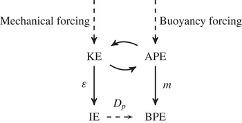
) due to laminar diffusion down the background gradient is negligible compared to the rate of increase in BPE due to turbulent mixing. The process described by these equations is illustrated by the diagram in figure 2. For a more detailed derivation of these equations see Peltier & Caulfield (Reference Peltier and Caulfield2003).
A simplified diagram of energy fluxes between kinetic energy (KE), available potential energy (APE), internal energy (IE) and background potential energy (BPE) in an incompressible, Boussinesq flow with a linear equation of state. In a closed system the source fluxes will be zero over the time interval defined by
 ${\it\Delta}$
(i.e. the forcing provides the initial energy for mixing, but is zero for
 $t>0$
).

The cumulative mixing efficiency
 ${\it\eta}$
in (2.6) is also equal to
 $$\begin{eqnarray}{\it\eta}=\frac{\displaystyle \int _{0}^{T}m\,\text{d}t}{\displaystyle \int _{0}^{T}(m+{\it\varepsilon})\,\text{d}t},\end{eqnarray}$$
where
 $T$
is a time scale that encapsulates a mixing event (Peltier & Caulfield Reference Peltier and Caulfield2003). An instantaneous mixing efficiency can be defined along the same lines,
 $$\begin{eqnarray}{\it\eta}_{i}=\frac{m}{m+{\it\varepsilon}}.\end{eqnarray}$$
In general,
 ${\it\eta}$
is not equal to the average instantaneous mixing efficiency,
 ${\it\eta}\neq (1/T)\int _{0}^{T}{\it\eta}_{i}\,\text{d}t$
. Moreover, a mixing event will usually occur over some finite time period and in this case the meaning of an instantaneous mixing efficiency would be somewhat questionable.
So far we have described only global, volumetric, energy-based measures to characterise the efficiency of mixing. Osborn (Reference Osborn1980) defined the local flux Richardson number as ‘the ratio of the buoyancy flux to the turbulent production’. Upon scaling and averaging the point-wise turbulent energy equations, Osborn (Reference Osborn1980) wrote the local flux Richardson number as
 $$\begin{eqnarray}Ri_{f}=\frac{-b^{\prime }}{-b^{\prime }+{\it\varepsilon}^{\prime }},\end{eqnarray}$$
where
 $b^{\prime }$
and
 ${\it\varepsilon}^{\prime }$
are defined at a point in space, rather than for a volume (see also Turner Reference Turner1973; Linden Reference Linden1979; Ivey & Imberger Reference Ivey and Imberger1991). Although the flux Richardson number
 $Ri_{f}$
and the instantaneous mixing efficiency
 ${\it\eta}_{i}$
share similarities in form, they are equal only in specific circumstances. The energy transfer
 $b^{\prime }$
does not differentiate between reversible and irreversible conversions to potential energy. Calculation of the efficiency of irreversible mixing is inherently non-local as it requires knowledge of the density field for the entire volume (so that we can find
 ${\it\Psi}({\it\rho})$
and calculate
 ${\rm\Delta}E_{b}$
). However, we expect the volume average of
 $Ri_{f}$
to be equal to the instantaneous mixing efficiency
 ${\it\eta}_{i}$
(and
 ${\it\eta}$
) for the special case of a domain that remains in a statistically steady state (Peltier & Caulfield Reference Peltier and Caulfield2003).
Mixing in ocean models is frequently parameterised in terms of the dissipation of local kinetic energy using the flux coefficient (also known as the mixing coefficient)
 $$\begin{eqnarray}{\it\gamma}=-b^{\prime }/{\it\varepsilon}^{\prime }.\end{eqnarray}$$
In general,
 ${\it\gamma}$
is defined as a local quantity, where
 $b^{\prime }$
and
 ${\it\varepsilon}^{\prime }$
are averaged at a point in space (Osborn Reference Osborn1980). Again,
 ${\it\gamma}$
is not guaranteed to differentiate between irreversible and reversible changes in the potential energy. We can relate the local
 $Ri_{f}$
and
 ${\it\gamma}$
as
 ${\it\gamma}=Ri_{f}/(1-Ri_{f})$
.
Confusingly, all three of
 $Ri_{f}$
,
 ${\it\gamma}$
and
 ${\it\eta}$
have been referred to as ‘the mixing efficiency’ in various papers, a situation not helped by a typical
 $Ri_{f}$
for mixing in a stably stratified shear flow being between
 $0.1$
and
 $0.2$
, a value small enough to make
 ${\it\gamma}\approx Ri_{f}$
. However, neither the flux Richardson number nor the flux coefficient are guaranteed to measure the irreversible increase of the potential energy associated with molecular diffusion. Moreover, the flux coefficient
 ${\it\gamma}$
does not correspond to an efficiency (on purely physical grounds) as it is not equal to the energy used for a particular purpose divided by the energy supplied to the system (instead
 $0\leqslant {\it\gamma}<\infty$
, whereas an efficiency
 $0\leqslant {\it\eta}\leqslant 1$
). We therefore refer throughout this paper to
 ${\it\eta}$
as the mixing efficiency.
3. Properties of mixing efficiency
Some key properties of the mixing efficiency defined by (2.6) can be illustrated by considering a class of flows – specifically types of Rayleigh–Taylor instability – where the initially available energy is all APE. Rayleigh–Taylor instability occurs in a flow when the pressure gradient
 $\boldsymbol{{\rm\nabla}}p$
opposes the density gradient
 $\boldsymbol{{\rm\nabla}}{\it\rho}$
, i.e.
 $\boldsymbol{{\rm\nabla}}p\boldsymbol{\cdot }\boldsymbol{{\rm\nabla}}{\it\rho}<0$
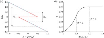
(Rayleigh Reference Rayleigh1883; Taylor Reference Taylor1950). In the example flows that follow, the instability is confined within an overall stable ambient stratification (e.g. figure 3
a). An important parameter for this type of density profile is the neutral buoyancy height
 $z_{n}$
, defined to be half the range of heights over which the density profile would change if the profile were sorted by density (essentially the length scale of the stratification).
(a) Example linear density profile with unstable interface (solid line) and the perfect mixing profile (dashed line), and the neutral buoyancy height
 $z_{n}$
and perfect mixing height
 $z_{p}$
. (b) Variation of mixing efficiency,
 ${\it\eta}$
, with normalised height of calculation
 $H/z_{n}$
.

The reason that this class of flows is so useful is that they have a well-defined final density profile, observed in both laboratory experiments (Lawrie & Dalziel Reference Lawrie and Dalziel2011b
; Davies Wykes & Dalziel Reference Davies Wykes and Dalziel2014) and numerical simulations (Lawrie & Dalziel Reference Lawrie and Dalziel2011b
). Specifically, laboratory experiments (with a fluid assumed to be miscible with a linear equation of state) have a final density profile very close to the one that we will refer to as the perfect mixing profile. This density profile has a central region of uniform density that extends to
 $-z_{p}\leqslant z\leqslant z_{p}$
, where
 $z_{p}$
is the perfect mixing height (e.g. figure 3
a). This coincides with the minimum height over which the fluid could interact to produce a stable stratification. Because this flow has easily defined initial and final states, it is relatively simple to calculate the mixing efficiency analytically, making it ideal for our purposes.
3.1. Mixing efficiency depends on regions remote from where mixing takes place
We will now return to the two idealised experiments plotted in figure 1. In the first experiment, we set up in a tank the unstable density profile shown in figure 1(a). The final density profile, measured when there is no remaining kinetic energy, will be the dashed line in figure 1(a) (known from the results of both laboratory experiments and simulations, as has been described above). Calculating the mixing efficiency from the initial and final density profiles, we find
 ${\it\eta}=3/4$
.
Now we will perform a second experiment, keeping the density gradients and discontinuity the same, but using a smaller tank (as plotted in figure 1
b). We reduce the volume of the experiment to only contain the mixing region, leaving out all the parts of the volume which do not change between the initial and final state. The initial density profile matches the profile in figure 1(a) over
 $-z_{p}\leqslant z\leqslant z_{p}$
and the final state is well-mixed, exactly as it was for the same range in the first experiment. When we calculate the mixing efficiency of this second experiment, we find
 ${\it\eta}=2/3$
.
Our two experiments have identical net changes in gravitational potential energy and therefore the viscous dissipation must be the same for both flows. The mixing is also identical (i.e. there is the same change in the volume of each density class) and yet, despite these similarities, the two flows have different values of mixing efficiency. We would observe the same behaviour if, instead of using a smaller tank, we replaced the stratified layers outside the mixing region with stable layers composed of densities outside the range of those present in the mixing region and which were not involved in the turbulent flow.
We could perform a series of experiments, each in a different sized tank (where the tank boundaries are situated at
 $z=\pm H$
). If
 $H$
is varied, the mixing efficiency
 ${\it\eta}$
changes as shown in figure 3(b). For these calculations, the density profile is sorted across
 $\pm H$
to find the BPE. For
 $|H|<z_{p}$
the flow changes in a fundamental way as the amount of mixing and change in potential energy no longer remain the same; we shall not pursue this limit further. The efficiency is seen to increase with
 $H$
until
 $H=z_{n}$
, beyond which there is no further dependence. These examples demonstrate that mixing efficiency is influenced by regions of the flow (here,
 $z_{p}<|z|\leqslant z_{n}$
) that do not change from the initial state and are not part of the turbulent mixing. This effect could be removed by always calculating the mixing efficiency only in the volume that changes from the initial conditions. However, calculating the mixing efficiency only across the mixing region artificially restricts the available energy that could be released. Thus the minimum calculation height for the mixing efficiency is the neutral buoyancy height,
 $z_{n}$
.
There are more general examples of flows where turbulent motions occur for
 $|z|>z_{n}$
, requiring extension of the principles above. In this case, the calculation height must be increased beyond
 $z_{n}$
to include all the region that can change from the initial conditions. One example is a three-layer flow with one Rayleigh–Taylor unstable interface and one stable interface (Jacobs & Dalziel Reference Jacobs and Dalziel2005). Only the two Rayleigh–Taylor unstable layers are swapped in the sorted density profile. However, Jacobs & Dalziel (Reference Jacobs and Dalziel2005) found that, in experiments, turbulence generated in the unstable region entrained fluid across the stable interface and the final mixing region extended slightly further than
 $z_{n}$
. In this case, the mixing efficiency should be based on the region that has mixed, but only because this is larger than
 $z_{n}$
.
Another example is when the initial conditions contain kinetic energy as well as APE. The above principle suggests that the calculation volume for
 ${\it\eta}$
should be the larger of
 $H=z_{n}$
and the height to which the turbulent motions could extend (aided by the initial KE). A priori determination of this height is a complicated function of the flow. However, in both examples
 ${\it\eta}$
should become independent of
 $H$
for sufficiently large
 $H$
, and this can provide a posteriori validation of the calculation.
There is class of flows for which
 $z_{n}$
is defined by the height of the domain. Examples include a buoyant plume rising in a homogeneous (or ‘weakly’ stratified) fluid, convection in either a homogeneous fluid or a sufficiently weak stratification and horizontal convection (Gayen et al.
Reference Gayen, Griffiths, Hughes and Saenz2013; Gayen, Griffiths & Hughes Reference Gayen, Griffiths and Hughes2014). In these cases, the flow is contained by the domain boundaries and the mixing efficiency calculation must involve (and is therefore a function of) the entire domain.
We can construct flows with identical mixing and identical dissipation of kinetic energy and yet different mixing efficiencies because of how we defined ‘energy used in mixing’. The background potential energy is a function of the global density profile, regardless of whether a region is turbulent or participates directly in the flow. To explain this further we will use a second example.
3.2. Removal of APE in regions remote from mixing
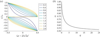
We have seen in § 3.1 that the mixing efficiency depends on the density profile outside the region where mixing physically occurs. We will examine this further by considering an initial (general polynomial) profile of the form
 $$\begin{eqnarray}\frac{{\it\rho}-\overline{{\it\rho}}}{{\it\rho}^{\prime }}=\left\{\begin{array}{@{}ll@{}}\displaystyle \frac{1}{2}-\left(\frac{z}{z_{n}}\right)^{q}\quad & \text{if }z\geqslant 0,\\ -\displaystyle \frac{1}{2}+\left(\frac{-z}{z_{n}}\right)^{q}\quad & \text{if }z<0,\end{array}\right.\end{eqnarray}$$
where
 $q>0$
(see figure 4(a) for a range of profiles with
 $q$
between
 $0.2$
and
 $2$
) and
 ${\it\rho}^{\prime }$
(
 ${>}0$
) is the maximum perturbation from the mean density
 $\overline{{\it\rho}}$
.
(a) Density profile with varying
 $0.2\leqslant q\leqslant 2$
. (b) The variation of mixing efficiency with
 $q$
, over the neutral buoyancy height
 $\pm z_{n}$

We assume that the final density profile is the perfect mixing profile described earlier (a result consistent with the experiments of Davies Wykes & Dalziel (Reference Davies Wykes and Dalziel2014)), with a constant-density region that is symmetric around the initially unstable interface and a perfect mixing height of
 $z_{p}=z_{n}\times 2^{-1/q}$
. The mixing efficiency calculated for
 $H\geqslant z_{n}$
is
 $$\begin{eqnarray}{\it\eta}_{z_{n}}=1-\frac{q^{2}}{\sqrt{{\rm\pi}}(q+2)}\frac{{\rm\Gamma}\left(\displaystyle \frac{3}{2}+\displaystyle \frac{1}{q}\right)}{{\rm\Gamma}\left(\displaystyle \frac{1}{q}\right)},\end{eqnarray}$$
where
 ${\rm\Gamma}$
is the Gamma function. The variation of
 ${\it\eta}_{z_{n}}$
with
 $q$
is plotted on figure 4(b). As
 $q\rightarrow 0$
and the mixing region becomes very thin (
 $z_{p}\rightarrow 0$
),
 ${\it\eta}_{z_{n}}$
tends to 1. As
 $q\rightarrow \infty$
, the mixing efficiency
 ${\it\eta}_{z_{n}}$
tends to
 $1/2$
(the maximum mixing efficiency for a monotonic, gravitationally unstable profile, see the Appendix).
In the examples shown in figures 3(a) and 4(a), there are parcels of fluid (outside the mixing region) that do not move or change in density between the initial and final states and whose contribution to APE in the initial state (from the gravitational instability) vanishes in the globally stable final state. The removal of APE and increase in BPE is normally viewed as a consequence of diffusion of solute from one fluid parcel to another, a process involving internal energy (Tailleux Reference Tailleux2013). However, the removal of APE in parts of the volume which are remote from the turbulent mixing region, a process we term ‘relabelling’, does not involve this pathway, does not require the local fluid to move and is a consequence of physical mixing elsewhere. This initially available energy becomes dynamically inaccessible to the flow because the profile becomes stable before that energy can be released. The example in figure 4(a) shows how, as the height of the mixing region becomes small relative to the neutral buoyancy height of the stratification (i.e.
 $q\rightarrow 0$
), the mixing efficiency tends to
 ${\it\eta}=1$
. Thus as
 $q$
decreases, a greater proportion of the initial available potential energy is relabelled and becomes inaccessible to the flow.
4. Pulse profile
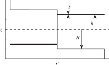
We will now describe a final example which we have called a ‘pulse’ profile (figure 5). This consists of a relatively dense sheet of fluid some distance above a relatively light sheet of fluid in an otherwise stable region of constant density,
 $$\begin{eqnarray}\frac{{\it\rho}-\overline{{\it\rho}}}{{\it\rho}^{\prime }}=\left\{\begin{array}{@{}ll@{}}-1\quad & \displaystyle \text{if }z\geqslant H\text{ or }-\!\left(h-\frac{{\it\delta}}{2}\right)\geqslant z>-\left(h+\frac{{\it\delta}}{2}\right),\\ 1\quad & \displaystyle \text{if}\left(h+\frac{{\it\delta}}{2}\right)\geqslant z>\left(h-\frac{{\it\delta}}{2}\right)\text{ or }z<-H,\\ 0\quad & \text{elsewhere,}\end{array}\right.\end{eqnarray}$$
where
 ${\it\delta}/2<h<H-{\it\delta}/2$
define the range of heights that the pulse centres can occupy, and thus the magnitude of the APE released into the flow. In this case the neutral density height
 $z_{n}$
is equal to
 $H$
. If the final state is the perfect mixing profile (i.e. well-mixed over the interval
 $\pm H$
) and the pulses of unstable fluid are much thinner than the neutral buoyancy height (
 ${\it\delta}\ll 2H$
) then
 $$\begin{eqnarray}{\it\eta}=\frac{1}{1+h/H}.\end{eqnarray}$$
A pulse profile consisting of pulses of relatively dense and light fluid, each of thickness
 ${\it\delta}$
and at heights
 $\pm h$
from the origin, suspended in a volume of total height
 $H$
.

For the purpose of calculating mixing efficiency in this example, the effect of changing the calculation height
 $H$
(or alternatively, the height of the experiment) and the density profile (by varying
 $h$
) are equivalent. If
 $h=H-{\it\delta}/2$
, then we find
 ${\it\eta}=1/2$
, the maximum mixing efficiency for any monotonic unstable density profile (see the Appendix). If
 $h\rightarrow {\it\delta}/2$
(two pulses situated either side of the origin), then
 ${\it\eta}\rightarrow 1$
. If the final profile is assumed to be well-mixed, the mixing efficiency is determined by the amount of energy we add (above the minimum APE requirement) by increasing
 $h$
. If we add the minimum amount of APE, we have a mixing efficiency of
 ${\it\eta}=1$
. If we add more APE, the mixing efficiency decreases as there is no more mixing that can occur (the final state already being well-mixed) and the additional APE must be dissipated. Therefore the mixing efficiency is lowered as
 $h$
increases.
5. Conclusions
Mixing in a density stratified fluid is typically confined to localised turbulent regions which are intermittent (or transient) in nature. It has been common practice to measure homogenisation of the density field in terms of the change in background potential energy, which can be defined formally with an energetics framework developed for such flows (Winters et al.
Reference Winters, Lombard, Riley and D’Asaro1995). The relative importance of sinks of energy in the mechanical energy budget can be related by the mixing efficiency, its numerical value often viewed as characterising the stratified turbulence, e.g. ‘mixing efficiency … seeks to provide a number quantifying the ability of a particular turbulent mixing event in dissipating [mechanical energy] ME
 $=$
APE
 $+$
KE preferentially diffusively rather than viscously’ (Tailleux Reference Tailleux2009).
In this paper we have shown that the mixing efficiency can depend on the density profile in regions of the flow that are neither turbulent nor undergo any physical mixing. Although the density profile remains unmodified in such regions, local fluid parcels can be associated with available potential energy in the initial state that is no longer present in the final state. This removal of available potential energy is a result of physical mixing elsewhere, which renders the initial available potential energy of such parcels dynamically inaccessible to the flow. For flows that are initially gravitationally stable (no initial available potential energy) and in which mixing is supported by the initial kinetic energy, the cumulative mixing efficiency between gravitationally stable initial and final states will not depend on the density profile outside the mixing region. However, the cumulative mixing efficiency between the start and some intermediate time could be affected by the density profile outside the region of physical mixing as all turbulent flows in which stratified mixing occurs must develop available potential energy at some point.
When mixing is confined by stratification (the main focus in this paper), a mixing efficiency that is independent of the volume of interest can be defined only if that volume is at least as large as the region affected by an adiabatic rearrangement of the initial density field to a statically stable state (i.e. sorted by density). In more general stratified flows, where mixing can occur outside the region estimated from adiabatic rearrangement, the mixing efficiency is well-defined only for volumes larger than that which incorporates any changes to the density field from the initial state. In some flows, such as convection or plumes, where the region in which sorting can occur is restricted only by the fluid domain, the mixing efficiency will be a function of the size of this domain.
There are other situations where the choice of calculation volume affects the calculated mixing efficiency. This can occur in stably stratified flows where there is a high spatial variability in the mixing, such as in the research of Hult et al. (Reference Hult, Troy and Koseff2011b ). They found that although there were regions of efficient mixing, when using a calculation volume that encompassed the whole flow, the mixing efficiency decreased as they were including regions of high dissipation without significant density gradients. This is in contrast to the examples we have described here where using a calculation volume that encompasses regions of the flow that do not change from the initial conditions increases the mixing efficiency due to a combined effect on the background and available potential energy.
Mixing in a closed domain can be expressed generally in terms of a change in the p.d.f. of density. An important general conclusion of this paper is that measures of mixing based on the energetics, including the mixing efficiency, must be regarded as quantities that can only be well-defined in a global sense. For instance, the change in background potential energy is not only a function of the change in the p.d.f., but also the p.d.f. itself. Moreover, we have shown that flows exist where, due to how the mixing efficiency
 ${\it\eta}$
is defined, it is possible to change the value of
 ${\it\eta}$
without changing the turbulent flow or amount of homogenised fluid. Our results highlight the need to consider alternative methods of characterising stratified mixing in such cases.
These results have significant implications for how mixing efficiency and energetics-based measures of mixing are used in oceanography where, rather than global density fields, only point and profile field measurements are typically available. It is often assumed that dissipation of available potential energy by mixing is equal to some fraction of the kinetic energy dissipation on a point-wise basis, in order to deduce the diapycnal mass diffusion from measurements of kinetic energy dissipation (i.e. using the flux Richardson number
 $Ri_{f}$
or flux coefficient
 ${\it\gamma}$
). This assumption almost certainly breaks down where gravitationally unstable regions are present, as has been demonstrated here. New methods of parameterising stratified mixing in a form suitable for use in the point-wise equations is an important area for future work.
Acknowledgements
G.O.H. was supported by Australian Research Council Future Fellowship FT100100869 and was hosted by DAMTP during this work. M.S.D.W. was funded by EPSRC (grant no. EP/P505445/1) and an AWE CASE award (AWE contract no. 30174006). This work is © British Crown Copyright 2014/AWE. This paper does not rely on data or other information beyond what is contained within this paper and the references cited herein.
Appendix. Maximum mixing efficiency for a one-dimensional gravitationally unstable monotonic stratification
The maximum mixing efficiency for any one-dimensional gravitationally unstable monotonic stratification is
 ${\it\eta}=1/2$
. The initial background potential energy for
 ${\it\rho}=f(z)$
, where
 $z=0$
is the mid-depth of the domain, can be calculated upon substituting the sorted profile
 $\hat{{\it\rho}}=f(-z)$
into (2.2). The initial background potential energy
 $E_{b}=-E_{p}$
(the initial gravitational potential energy) and the initial available potential energy
 $E_{a}=2E_{b}$
. A well-mixed final state has gravitational potential energy
 $E_{p}=0$
, as the well-mixed region is symmetric about the origin. This results in a mixing efficiency of
 ${\it\eta}=1/2$
. This is the maximum possible mixing efficiency because no more mixing can occur (we cannot do better than a well-mixed state). This result holds regardless of the exact analytical form of
 $f(z)$
.