2.1. The non-dimensional equations and multiple scales approach

The two-dimensional rSWE, in dimensional form and linearised about a state of rest, are

(2.1)\begin{equation} \left.\begin{gathered} \boldsymbol{u}_t + f \boldsymbol{k} \times \boldsymbol{u} ={-} g \boldsymbol{\nabla} \eta, \\ \eta_t + \boldsymbol{\nabla}\boldsymbol{\cdot} (h \boldsymbol{u}) = 0. \end{gathered}\right\} \end{equation}

Here, $ \boldsymbol {u}$ is the horizontal velocity and $\eta$ the free-surface displacement, $ \boldsymbol {k}$ is the unit vector in the vertical direction, $h$ is the depth of the undisturbed ocean which varies on a horizontal scale $l$ due to the presence of bottom topography, $f=f_0+\beta y$ is the local Coriolis parameter, with $\beta$ denoting the Rossby parameter, and $g$ is the acceleration due to gravity.

In order to apply asymptotic analysis consistently, it is convenient to work with non-dimensional equations. It will be assumed in all that follows that $l \ll L, L_\beta$, where $L=\sqrt {gH_0}/f_0$ is the Rossby radius and $L_\beta =f_0/\beta$ is the length scale associated with the planetary vorticity gradient. Since our interest here is in waves with wavelength longer than $l$, it is convenient to take the Rossby radius $L$ as our horizontal scale, and to treat the non-dimensional parameter $b=L/L_\beta$ as order unity. Choosing a time scale $f_0^{-1}$, a velocity scale $U$, and free-surface displacement scale $f_0 U L /g$, the non-dimensional equations are found to be

(2.2)\begin{equation} \left.\begin{gathered} \boldsymbol{u}_t + (1+ b y) \boldsymbol{k} \times \boldsymbol{u} ={-} \boldsymbol{\nabla} \eta, \\ \eta_t + \boldsymbol{\nabla}\boldsymbol{\cdot} (h \boldsymbol{u}) = 0. \end{gathered}\right\} \end{equation}

For ease of notation in (2.2), the same variable names have been retained as for their dimensional counterparts in (2.1). Notice that the velocity scale $U$ in the treatment above is arbitrary, except that it must be sufficiently small for the linear equations to remain valid.

Below, we will also make use of the linear potential vorticity (PV) equation, which follows from (2.2) by taking the curl of the momentum equation and then substituting in the continuity equation

(2.3)\begin{equation} \frac{1}{h} \frac{\partial}{\partial t} \left( \zeta - \frac{(1+by) \eta}{h} \right) + \boldsymbol{u} \boldsymbol{\cdot}\boldsymbol{\nabla} \left( \frac{1+by}{h} \right) = 0,\end{equation}

where $\zeta = \boldsymbol {k} \boldsymbol {\cdot }\boldsymbol {\nabla } \times \boldsymbol {u}$ is the relative vorticity.

To exploit the horizontal scale separation between the topography and the length scales of the waves of interest, a small parameter $\varepsilon = l / L \ll 1$ can now be introduced. To permit multiple-scale analysis, the spatial variable $ \boldsymbol {X}= \boldsymbol {x}/ \varepsilon$ can be defined, which describes spatial variations on the scale of the topography. Importantly, we treat $ \boldsymbol {x}$ and $ \boldsymbol {X}$ as independent variables in the following analysis. In general, the topography $h( \boldsymbol {X}, \boldsymbol {x})$ can also be allowed to vary on the long length scale associated with $ \boldsymbol {x}$, as would be useful for example to describe a large-scale topographic slope covered in small-scale seamounts.

Next, we introduce an average $\langle \cdot \rangle$ over the short scales, which can be applied to any function $g( \boldsymbol {X}, \boldsymbol {x})$,

(2.4)\begin{equation} \langle g \rangle = \frac{1}{|\varOmega|} \int_\varOmega g(\boldsymbol{X},\boldsymbol{x})\,\textrm{d}\boldsymbol{X}. \end{equation}

In the following sections, two main cases will be considered. The first, most tractable case, is that of a regular periodic lattice of seamounts, in which case $\varOmega$ is a single doubly periodic cell ($|\varOmega |$ denotes its area). The second case is that of randomly distributed topography, in which case $\varOmega$ can be taken to be a spatial average over a ‘mesoscale’ region which is (asymptotically) intermediate in size between the small and large scales. In the asymptotic limit, the number of mountains in the mesoscale region will tend to infinity, and the mesoscale average will be independent of the particular distribution of the topography and will therefore be equivalent to an ensemble average. The analysis which follows in the rest of this section applies equally in both regimes. Averaged variables will be denoted below by capitals, e.g. applying the spatial average to the topography gives

(2.5)\begin{equation} H(\boldsymbol{x})= \langle h(\boldsymbol{X},\boldsymbol{x}) \rangle. \end{equation}

Finally, replacing horizontal derivatives according to the multi-scale formalism, using the chain rule (i.e. $\boldsymbol {\nabla } \to \varepsilon ^{-1} \boldsymbol {\nabla }_{ \boldsymbol {X}} + \boldsymbol {\nabla }_{ \boldsymbol {x}}$) gives

(2.6)\begin{equation} \left.\begin{gathered} \varepsilon \boldsymbol{u}_t + \varepsilon (1+by) \boldsymbol{k} \times \boldsymbol{u} ={-} \boldsymbol{\nabla}_{\boldsymbol{X}} \eta - \varepsilon \boldsymbol{\nabla}_{\boldsymbol{x}} \eta, \\ \varepsilon \eta_t + \boldsymbol{\nabla}_{\boldsymbol{X}} \boldsymbol{\cdot} (h \boldsymbol{u})+ \varepsilon \boldsymbol{\nabla}_{\boldsymbol{x}} \boldsymbol{\cdot} (h \boldsymbol{u}) = 0. \end{gathered}\right\} \end{equation}

The equations (2.6) are the starting point for the analysis to follow.

2.2. The homogenised equations

The large-scale homogenised equations can be obtained from (2.6) by seeking a multiple-scale perturbation solution of the form

(2.7)\begin{equation} \left.\begin{gathered} \eta(\boldsymbol{X},\boldsymbol{x},t; \varepsilon) = \eta_0(\boldsymbol{X},\boldsymbol{x},t)+\varepsilon \eta_1(\boldsymbol{X},\boldsymbol{x},t)+\cdots \\ \boldsymbol{u}(\boldsymbol{X},\boldsymbol{x},t; \varepsilon) = \boldsymbol{u}_0(\boldsymbol{X},\boldsymbol{x},t)+\varepsilon \boldsymbol{u}_1(\boldsymbol{X},\boldsymbol{x},t)+\cdots. \end{gathered}\right\} \end{equation}

Inserting (2.7) in (2.6) gives, at leading order

(2.8a,b)\begin{equation} \boldsymbol{\nabla}_{\boldsymbol{X}} \eta_0=0,\quad \boldsymbol{\nabla}_{\boldsymbol{X}} \boldsymbol{\cdot} ( h \boldsymbol{u}_0)=0. \end{equation}

From this we deduce that $\eta _0=\varPi ( \boldsymbol {x},t)$ is independent of the small-scale variable $ \boldsymbol {X}$ (i.e. $\eta _0=\langle \eta _0\rangle := \varPi$), and that

(2.9)\begin{equation} \boldsymbol{u}_0(\boldsymbol{X},\boldsymbol{x},t) = \frac{\boldsymbol{U} H + \boldsymbol{\nabla}^{{\perp}}_{\boldsymbol{X}} \psi}{h}, \end{equation}

where $\boldsymbol {\nabla }^{\perp }_{ \boldsymbol {X}} \equiv \boldsymbol {k}\times \boldsymbol {\nabla }_{ \boldsymbol {X}}$ is the skew-gradient operator, and

(2.10)\begin{equation} \boldsymbol{U}(\boldsymbol{x},t)= \frac{\langle \boldsymbol{u}_0 h \rangle}{\langle h \rangle} \end{equation}

is the depth-weighted average velocity. Here $\psi ( \boldsymbol {X}, \boldsymbol {x},t)$ is an unknown scalar function to be determined.

Next, applying the averaging operator to the multi-scale equations (2.6), after multiplying the momentum equation by $h$, gives, at leading order

(2.11)\begin{equation} \left.\begin{gathered} \boldsymbol{U}_t + (1+by) \boldsymbol{k} \times \boldsymbol{U} ={-} \boldsymbol{\nabla}_{\boldsymbol{x}} \varPi + \frac{\langle \eta_1 \boldsymbol{\nabla}_{\boldsymbol{X}}h \rangle }{H}, \\ \varPi_{t} + \boldsymbol{\nabla}_{\boldsymbol{x}} \boldsymbol{\cdot} \left( H \boldsymbol{U} \right) = 0. \end{gathered}\right\} \end{equation}

Equations (2.11) govern the evolution of long waves in the presence of topography, except that to close the equations it remains necessary to evaluate the correlation term $\langle \eta _1 \boldsymbol {\nabla }_{ \boldsymbol {X}}h \rangle$ in terms of the averaged variables $ \boldsymbol {U}$, $\varPi$ and $H$.

To evaluate the correlation term $\eta _1$ must be determined, and to do so it is necessary to consider the momentum equation of (2.6) at next order. Multiplying by $h$ and taking the divergence $\boldsymbol {\nabla }_{ \boldsymbol {X}} \boldsymbol {\cdot } (\cdot )$, gives

(2.12)\begin{equation} \boldsymbol{\nabla}_{\boldsymbol{X}} \boldsymbol{\cdot} \left( h \boldsymbol{\nabla}_{\boldsymbol{X}} \eta_1 \right) - (1+by) \boldsymbol{\nabla}_{\boldsymbol{X}}^{2} \psi ={-} \boldsymbol{\nabla}_{\boldsymbol{X}} h \boldsymbol{\cdot} \boldsymbol{\nabla}_{\boldsymbol{x}} \varPi. \end{equation}

This is an elliptic equation for $\eta _1$ which involves the other unknown function $\psi$. Evidently another equation is needed to close the system, which can be determined most easily from the PV equation (2.3), which at leading order in $\varepsilon$ is

(2.13)\begin{align} \boldsymbol{\nabla}_{\boldsymbol{X}} \boldsymbol{\cdot} \left( \frac{\boldsymbol{\nabla}_{\boldsymbol{X}} \psi_t}{h} \right) - (1+by) \boldsymbol{\nabla}_{\boldsymbol{X}} \psi \boldsymbol{\cdot}\boldsymbol{\nabla}_{\boldsymbol{X}}^{{\perp}} \left(\frac{1}{h}\right) ={-} H \left((1+by) \boldsymbol{U} -\boldsymbol{k} \times \boldsymbol{U}_t \right) \boldsymbol{\cdot}\boldsymbol{\nabla}_{\boldsymbol{X}}\left(\frac{1}{h}\right).\end{align}

Notice that (2.12) and (2.13) have both been written with terms involving the unknown $\psi$ and $\eta _1$ on the left, and ‘source’ terms involving $h$ and the averaged variables on the right. Before $\eta _1$ can be found in terms of the sources from (2.12), (2.13) must first be solved for $\psi$. The time dependence in (2.13) is an expected feature, and arises because the rotation adds new physics to the shallow water equations, namely that topography at any horizontal scale will support the motion of trapped topographic Rossby waves (Longuet-Higgins Reference Longuet-Higgins1967; Jansons & Johnson Reference Jansons and Johnson1988). As discussed in the quasi-geostrophic context by Vanneste (Reference Vanneste2000b) and Benilov (Reference Benilov2000), these trapped Rossby waves can be excited resonantly by the large-scale motion.

In general, because (2.12)–(2.13) are linear in $\psi$ and $\eta _1$, the solution for $\eta _1$ can be expressed formally using a Green's function approach, in the form of history integral over the past state of the system. This approach, broadly following that of (Vanneste Reference Vanneste2000a), is followed in Appendix B, and results in an integro-differential equation (B6) for the time-evolution of the momentum $ \boldsymbol {U}$.

However, our primary interest here is in the impact of the topography on the dispersion relations of periodic waves, therefore solutions $\propto \exp {(-\textrm {i}\omega t)}$ will henceforth be sought, allowing the substitution $\partial _t \to -\textrm {i}\omega$. It follows that (2.13) becomes

(2.14)\begin{align} \boldsymbol{\nabla}_{\boldsymbol{X}} \boldsymbol{\cdot} \left( \frac{\boldsymbol{\nabla}_{\boldsymbol{X}} \psi}{h} \right) - \mathrm{i} \frac{1+by}{\omega} \boldsymbol{\nabla}_{\boldsymbol{X}} \psi \boldsymbol{\cdot} \boldsymbol{\nabla}_{\boldsymbol{X}}^{{\perp}}\left(\frac{1}{h}\right) ={-} H \left(\mathrm{i} \frac{1+by}{\omega} \boldsymbol{U}-\boldsymbol{k} \times \boldsymbol{U} \right) \boldsymbol{\cdot}\boldsymbol{\nabla}_{\boldsymbol{X}}\left(\frac{1}{h}\right), \end{align}

and the solution $\eta _1$ of (2.12) and (2.14) can be expressed as

(2.15)\begin{equation} \eta_1 = \boldsymbol{\varPhi} \boldsymbol{\cdot}\boldsymbol{\nabla}_{\boldsymbol{x}} \varPi + H(1+by) \boldsymbol{\varPsi}_{(1+by)/\omega} \cdot \left(\mathrm{i}\frac{1+by}{\omega} \boldsymbol{U} -\boldsymbol{k}\times\boldsymbol{U} \right). \end{equation}

In (2.15) the vectors $ \boldsymbol {\varPhi }=(\varPhi _1,\varPhi _2)^{\textrm {T}}$ and $ \boldsymbol {\varPsi }_\alpha =(\varPsi _{1,\alpha },\varPsi _{2,\alpha })^{\textrm {T}}$ are obtained by solving the so-called ‘cell problems’

(2.16)\begin{equation} \boldsymbol{\nabla}_{\boldsymbol{X}}\boldsymbol{\cdot} \left( h \boldsymbol{\nabla}_{\boldsymbol{X}} \varPhi_i \right) ={-} \partial_{X_i} h, \end{equation}

and

(2.17)\begin{equation} \left.\begin{gathered} \boldsymbol{\nabla}_{\boldsymbol{X}} \boldsymbol{\cdot} \left( h \boldsymbol{\nabla}_{\boldsymbol{X}} \varPsi_{i,\alpha} \right) = \boldsymbol{\nabla}_{\boldsymbol{X}} ^{2} G_i, \\ \boldsymbol{\nabla}_{\boldsymbol{X}} \boldsymbol{\cdot} \left( \frac{\boldsymbol{\nabla}_{\boldsymbol{X}} G_i}{h} \right) - \textrm{i} \alpha \boldsymbol{\nabla}_{\boldsymbol{X}} G_i \boldsymbol{\cdot} \boldsymbol{\nabla}_{\boldsymbol{X}}^{{\perp}} \left( \frac{1}{h} \right) ={-} \partial_{X_i} \left( \frac{1}{h} \right), \end{gathered}\right\} \end{equation}

respectively, where $\alpha >0$ is a parameter. The cell problems are elliptic equations defined on $\varOmega$, and have unique solutions up to arbitrary functions of the large-scale variables only (see e.g. § 5.3.2 of Holmes Reference Holmes2012). The arbitrary functions can be ignored since they do not contribute to the correlation term in (2.11).

It is important to emphasise that the solutions $ \boldsymbol {\varPhi }$ and $ \boldsymbol {\varPsi }_\alpha$ of the cell problems depend only on the details of the topography, not on the waves being studied or on dynamical parameters such as $b$. The first cell problem (2.16) is, for reasons to be explained below, identical to that most commonly arising in classical two-dimensional homogenisation problems of mathematical physics, such as heat transfer through heterogeneous media, the study of which dates back to Rayleigh (Reference Rayleigh1892). The second cell problem (2.17), which is perhaps more accurately described as a one-parameter family of cell problems parametrised by $\alpha$, is introduced by the presence of rotation and the associated topographic Rossby waves. An important point is that for real $\alpha$, $ \boldsymbol {\varPsi }_\alpha = \boldsymbol {\varPsi }_{-\alpha }^{*}$, as can be seen by making the substitutions $\alpha \rightarrow -\alpha$ and $G_i \rightarrow G_i^{*}$ (complex conjugate).

Inserting our expression for $\eta _1$ from (2.15) leads to

(2.18)\begin{align} & -\textrm{i}\omega \left(\boldsymbol{\mathcal{I}} + \left( \frac{1+by}{\omega} \right)^{2} \boldsymbol{\mathcal{K}}_{(1+by)/\omega} \right) \cdot \boldsymbol{U} + \left(1+by \right) \left( \boldsymbol{\mathcal{I}} + \boldsymbol{\mathcal{K}}_{(1+by)/\omega} \right) \cdot \boldsymbol{k} \times\boldsymbol{U} \nonumber\\ &\quad ={-}\left( \boldsymbol{\mathcal{I}} + \boldsymbol{\mathcal{D}} \right) \boldsymbol{\cdot}\boldsymbol{\nabla}_{\boldsymbol{x}}\varPi, \end{align}

where $ \boldsymbol {\mathcal {I}}$ is the identity matrix and the matrices $ \boldsymbol {\mathcal {D}}$ and $ \boldsymbol {\mathcal {K}}_\alpha$ are given by

(2.19a,b) \begin{equation} \boldsymbol{\mathcal{D}} ={-}\frac{1}{H} \left(\begin{array}{@{}cc@{}} \langle \varPhi_1 \partial_{X_1} h \rangle & \langle \varPhi_2 \partial_{X_1} h \rangle \\ \langle \varPhi_1 \partial_{X_2} h \rangle & \langle \varPhi_2 \partial_{X_2} h \rangle \end{array}\right),\quad \boldsymbol{\mathcal{K}}_\alpha = \left( \begin{array}{@{}cc@{}} \langle \varPsi_{1,\alpha} \partial_{X_1} h \rangle & \langle \varPsi_{2,\alpha} \partial_{X_1} h \rangle \\ \langle \varPsi_{1,\alpha} \partial_{X_2} h \rangle & \langle \varPsi_{2,\alpha} \partial_{X_2} h \rangle \end{array} \right). \end{equation}

For cell problems with a fourfold rotational symmetry, for example axisymmetric seamounts arranged in a regular square lattice, these matrices simplify to $ \boldsymbol {\mathcal {D}}=D \boldsymbol {\mathcal {I}}$ and

(2.20)\begin{equation} \boldsymbol{\mathcal{K}}_\alpha=\left(\begin{array}{@{}cc@{}} K_1(\alpha) & -\textrm{i} K_2(\alpha) \\ \textrm{i}K_2(\alpha) & K_1(\alpha) \end{array}\right), \end{equation}

for real, scalar functions $K_1(\alpha )$ and $K_2(\alpha )$, which hereafter we will call the ‘topographic resonance functions’. The cell-averaged linear rSWE then simplify to

(2.21)\begin{equation} \left.\begin{gathered} -\textrm{i}\omega \left( 1 + \left( \frac{1+by}{\omega} \right)^{2} K_1 \left(\frac{1+by}{\omega}\right)+ \left( \frac{1+by}{\omega} \right)K_2 \left(\frac{1+by}{\omega}\right) \right) \boldsymbol{U} \\ \quad + (1+by)\left( 1+ K_1\left(\frac{1+by}{\omega}\right)+ \left(\frac{1+by}{\omega} \right)K_2\left(\frac{1+by}{\omega}\right)\right)\boldsymbol{k} \times \boldsymbol{U}\\ ={-}(1+D) \boldsymbol{\nabla}_{\boldsymbol{x}} \varPi, \\ -\textrm{i}\omega\varPi + \boldsymbol{\nabla}_{\boldsymbol{x}} \boldsymbol{\cdot} \left( H \boldsymbol{U} \right) = 0, \end{gathered}\right\} \end{equation}

where again, we emphasise that $D$, $K_1(\alpha )$ and $K_2(\alpha )$ are properties of the topography alone.

The system of (2.21) can be solved to obtain expressions determining the dispersion relations of the Poincaré, Kelvin and Rossby waves solutions of the rSWE on the $\beta$-plane. In §§ 3 and 4 below numerical and analytical results are presented which illustrate the extent to which different topographies affect the dispersion relations of these waves. The results of this section have counterparts when Ekman friction is included in the governing equations, but for simplicity our main focus here is on the frictionless case. However, as in the quasi-geostrophic problem (Vanneste Reference Vanneste2000a,Reference Vannesteb), it is necessary to include a regularising process such as Ekman friction in order to make physical sense of behaviours when there is a resonance between the waves of interest and topographic Rossby waves on the seamounts. Other dissipative processes, such as eddy diffusivity of momentum, could also play a regularising role. Additionally, nonlinearity will also likely act to remove the singularity at the resonances as occurs in the theory of Bragg scattering of water waves (see e.g. the weakly nonlinear analysis of Hara & Mei Reference Hara and Mei1987). Here, following Vanneste (Reference Vanneste2000b), only Ekman friction is considered and in Appendix A the results above are generalised to include this effect. The analogue of the equations (2.21) are shown there to be (A12).

Next, we consider some relevant limits of (2.11) and (2.21).

2.3. Quasi-geostrophic limit of the homogenised equations

The quasi-geostrophic limit of the homogenised equations (2.11) can be obtained by considering the joint limit $b\ll 1$, in which $h=1 - b h_b$, i.e. deviations from a uniform depth of unity are small, and are described by the re-scaled bottom topography $h_b( \boldsymbol {X})$ (as for the full system, $h_b$ can be allowed to depend on $ \boldsymbol {x}$ if required). Time must also be rescaled to the slower timescale $T=b t$. Expanding

(2.22a,b)\begin{equation} \varPi= \varPi^{(0)}+b \varPi^{(1)}+b^{2} \varPi^{(2)}+\cdots,\quad \boldsymbol{U}=\boldsymbol{U}^{(0)}+ b \boldsymbol{U}^{(1)}+b^{2} \boldsymbol{U}^{(2)} + \cdots, \end{equation}

leads to geostrophic balance at leading order $-\boldsymbol {\nabla }_{ \boldsymbol {x}}\varPi ^{(0)}= \boldsymbol {k} \times \boldsymbol {U}^{(0)}$ (equivalently $ \boldsymbol {U}^{(0)}=\boldsymbol {\nabla }_{ \boldsymbol {x}}^{\perp } \varPi ^{(0)}$), and at next order

(2.23)\begin{equation} \left.\begin{gathered} \partial_T \boldsymbol{U}^{(0)} + \boldsymbol{k} \times \boldsymbol{U}^{(1)} + y \boldsymbol{k} \times \boldsymbol{U}^{(0)} ={-} \boldsymbol{\nabla}_{\boldsymbol{x}} \varPi^{(1)} - \langle \eta_1^{(0)} \boldsymbol{\nabla}_{\boldsymbol{X}}h_b \rangle, \\ \partial_T\varPi^{(0)} + \boldsymbol{\nabla}_{\boldsymbol{x}} \boldsymbol{\cdot} \boldsymbol{U}^{(1)} = 0. \end{gathered}\right\} \end{equation}

Applying $\boldsymbol {\nabla }_{ \boldsymbol {x}}^{\perp } \boldsymbol {\cdot }$ to the momentum equation in (2.23), and using the free-surface displacement equation to eliminate $\boldsymbol {\nabla }_{ \boldsymbol {x}} \boldsymbol {\cdot } \boldsymbol {U}^{(1)}$, leads to the quasi-geostrophic potential vorticity equation

(2.24)\begin{equation} \partial_T \left( \nabla^{2}_{\boldsymbol{x}} \varPi^{(0)} - \varPi^{(0)} \right) + \varPi_{x}^{(0)} + \boldsymbol{\nabla}_{\boldsymbol{x}} \boldsymbol{\cdot} \langle h_b \boldsymbol{\nabla}^{{\perp}}_{\boldsymbol{X}} \eta_1^{(0)} \rangle = 0. \end{equation}

Here, $\eta _{1}^{(0)}$ is determined by the leading-order terms in (2.12) and (2.13) which can be simplified to

(2.25)\begin{equation} \partial_T \boldsymbol{\nabla}_{\boldsymbol{X}}^{2} \eta_{1}^{(0)} - \boldsymbol{\nabla}_{\boldsymbol{X}} \eta_{1}^{(0)} \boldsymbol{\cdot}\boldsymbol{\nabla}_{\boldsymbol{X}}^{{\perp}} h_b = \boldsymbol{\nabla}_{\boldsymbol{x}} \varPi^{(0)} \boldsymbol{\cdot}\boldsymbol{\nabla}^{{\perp}}_{\boldsymbol{X}}h_b. \end{equation}

Equations (2.24) and (2.25) are the homogenised equations of the quasi-geostrophic system of Vanneste (Reference Vanneste2000a,Reference Vannesteb) in the absence of friction. If we seek solutions $\propto \exp (-\textrm {i}\varOmega T)$, where $\varOmega =\omega /b$ is the frequency on the slow time scale, then the solution $\eta _1^{(0)}$ is found from the leading-order terms in (2.15) to be

(2.26)\begin{equation} \eta_1^{(0)}=\frac{\textrm{i}}{\varOmega} \tilde{\boldsymbol{\varPsi}}_{1/\varOmega} \boldsymbol{\cdot} \boldsymbol{\nabla_{\boldsymbol{x}}}^{{\perp}} \varPi, \end{equation}

where the vector $\tilde { \boldsymbol {\varPsi }}_\alpha = \textrm {Re}(\tilde {\varPsi }_{1,\alpha },\tilde {\varPsi }_{2,\alpha })^{\textrm {T}}$ has components which solve the cell problem (2.17) at leading order in $b$,

(2.27)\begin{equation} \boldsymbol{\nabla}_{\boldsymbol{X}}^{2} \tilde{\varPsi}_{i,\alpha} -\textrm{i} \alpha \boldsymbol{\nabla}_{\boldsymbol{X}}\tilde{\varPsi}_{i,\alpha} \boldsymbol{\cdot}\boldsymbol{\nabla}_{\boldsymbol{X}}^{{\perp}} h_b ={-} \partial_{X_i} h_b.\end{equation}

Focusing on symmetric topography, defining $\tilde {K}(\alpha )=- \langle \tilde {\varPsi }_{1,\alpha } \partial _{X_1} h_b \rangle$ to be the quasi-geostrophic analogue of $K_1(\alpha )$ (the quasi-geostrophic analogue of $K_2(\alpha )$ vanishes), and then substituting $\varOmega = \omega / b$ allows the eigenvalue equation for the homogenised quasi-geostrophic system to be written as

(2.28)\begin{equation} -\textrm{i}\omega \left(1+\frac{b^{2}}{\omega^{2}}\tilde{K} \left(\frac{b}{\omega}\right)\right)\nabla_{\boldsymbol{x}}^{2}\varPi^{(0)}+\textrm{i}\omega \varPi^{(0)}+b\varPi_{x}^{(0)}=0,\end{equation}

recovering the result of Vanneste (Reference Vanneste2000a).

The derivation of (2.24)–(2.28) above differs from that of Vanneste (Reference Vanneste2000a) in a significant way. Here, we have obtained (2.24)–(2.28) by first deriving the homogenised equations (2.11) and then taking the quasi-geostrophic limit, corresponding to the following ordering of the small parameters: $\varepsilon \ll b \ll 1$. Vanneste, by contrast, applied the homogenisation procedure to the quasi-geostrophic equations themselves, consistent with the ordering $b \ll \varepsilon \ll 1$. The fact that the same equations are found in each case gives a clear indication that the result is independent of the value of the ratio $\varepsilon / b=l L_\beta / L^{2}$ (where $l$ is the topography length scale, $L$ is the Rossby radius and $L_\beta =f_0/\beta$). In fact, independence of $\varepsilon / b$ can be shown more explicitly by a direct asymptotic treatment of (2.6) with $\varepsilon \sim b$ (details not given here). In other words, there is no restriction on the topographic length scale $l$, beyond the shallow water scaling $l \gg H_0$, for (2.24)–(2.25) to hold, a result which extends that of Vanneste, which covers only the case $l \gg L^{2} / L_\beta$.

2.4. Non-rotating homogenised equations

To introduce our main results below, it is helpful to first consider (2.11) in the absence of rotation

(2.29)\begin{equation} \left.\begin{gathered} \boldsymbol{U}_t ={-} \boldsymbol{\nabla}_{\boldsymbol{x}} \varPi + \frac{\langle \eta_1 \boldsymbol{\nabla}_{\boldsymbol{X}}h \rangle}{H}, \\ \varPi_{t} + \boldsymbol{\nabla}_{\boldsymbol{x}} \boldsymbol{\cdot} \left( H \boldsymbol{U} \right) = 0, \end{gathered}\right\} \end{equation}

where in this case $\eta _1= \boldsymbol {\varPhi } \boldsymbol {\cdot }\boldsymbol {\nabla }_{ \boldsymbol {x}} \varPi$, with $ \boldsymbol {\varPhi }=(\varPhi _1,\varPhi _2)^{\textrm {T}}$, and $\varPhi _i$ is determined by the cell problem (2.16). In this case, taking the time derivative of the free-surface equation and substituting for $ \boldsymbol {U}_t$ results in the wave equation

(2.30)\begin{equation} \varPi_{tt} = \boldsymbol{\nabla}_{\boldsymbol{x}} \boldsymbol{\cdot} \left( H(\boldsymbol{\mathcal{I}} + \boldsymbol{\mathcal{D}} ) \boldsymbol{\cdot}\boldsymbol{\nabla}_{\boldsymbol{x}} \varPi \right), \end{equation}

with $ \boldsymbol {\mathcal {D}}$ given by (2.19a). The result (2.30) shows that, as expected, shallow water gravity waves obey the wave equation. For symmetric arrays of seamounts with $ \boldsymbol {\mathcal {D}}=D \boldsymbol {\mathcal {I}}$, the local gravity wave speed is given by $H_{eff}^{1/2}$, where $H_{eff}=H(1+D)$ is the non-dimensional effective depth (the dimensional units here being $\sqrt {gH_0})$. As discussed in the introduction, functional analysis techniques (e.g. Nandakumaran (Reference Nandakumaran2007), Allaire (Reference Allaire2012) and Mei & Vernescu (Reference Mei and Vernescu2010), § 5.5) applied to (2.30) when $ \boldsymbol {\mathcal {D}}=D \boldsymbol {\mathcal {I}}$ reveals the Reuss–Voigt bounds $\bar {H}\equiv \langle h^{-1} \rangle ^{-1} \le H_{eff} \le \langle h \rangle \equiv H$, with the lower (harmonic mean or Reuss) bound being attained exactly for propagation over a one-dimensional topography. In § 3.3 below the two-dimensional case is discussed in detail for the case of regular periodic arrays of circular cylinders.

3.1. The $\beta $-channel dispersion relation in the absence of topography

To set the scene for a quantitative assessment of topographic effects on the dispersion relations, it is helpful to recall the characteristics of Rossby, Kelvin and Poincaré waves in the flat-bottomed case. While (2.21) can be used to investigate wave dispersion in arbitrary domains, including bounded ocean basins and the equatorial $\beta$-plane, for definiteness we consider a semi-infinite midlatitude $\beta$-channel bounded by sidewalls at $y=\pm w$, where $w$ is the ratio of the half-width of the channel to the Rossby radius. The approach closely follows that of Paldor et al. (Reference Paldor, Rubin and Mariano2007) and Paldor & Sigalov (Reference Paldor and Sigalov2008) to which the reader is referred for more detail. The channel width parameter is set as $w=1$ hereafter, because, while it is the case that $w$ does affect the branches of the dispersion relation by determining the quantisation of the meridional wavenumber in the channel, varying $w$ is found to have a minimal effect on the relative change of each branch due to the topography.

In the absence of topography, $D=K_i(\alpha )=0$ and $H$ is constant in (2.21), and the equations can be simplified by eliminating $U$ and $\varPi$ to obtain

(3.1)\begin{equation} \nabla_{\boldsymbol{x}}^{2} V+\frac{1}{H}\left(\omega^{2}V-(1+by)^{2}V\right)+\textrm{i} \frac{b}{\omega}V_x=0. \end{equation}

Seeking periodic solutions in $x$ by substituting $V(x,y) \to V(y)\ \textrm {e}^{\textrm {i}kx}$ (abusing notation by retaining the variable name $V$) gives the Sturm–Liouville problem

(3.2)\begin{equation} \frac{{\textrm{d}}^{2} V}{{\textrm{d}y}^{2}}+\left( \frac{\omega^{2}}{H}- k^{2}- \frac{bk}{\omega}-\frac{(1+by)^{2}}{H}\right)V=0,\quad V({\pm} 1)=0. \end{equation}

The problem is standard once the Sturm–Liouville eigenvalues $\{E_n,\ n=1,2,3\cdots \}$ are identified with $E(\omega ,k)=\omega ^{2}/H-k^{2}-bk/\omega$. In general the $\{E_n\}$, which since $w$ is fixed depend only on $b$, can be calculated numerically and the Poincaré and Rossby branches of the dispersion relation follow from finding the roots of the cubic

(3.3)\begin{equation} \frac{\omega^{2}}{H}-k^{2}-\frac{bk}{\omega}=E_n(b). \end{equation}

The Kelvin wave, which has $V=0$ everywhere, is solved for separately and has dispersion relation $\omega =\sqrt {H}k$.

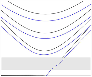
Figure 1 (dotted curves) shows the first three branches of the dispersion relation, obtained from (3.3) after solving (3.2) to obtain $E_1$, $E_2$ and $E_3$ using a standard Chebyshev spectral discretisation (e.g. Trefethen (Reference Trefethen2000), 48 points are used), for parameters $b=0.5$ and $H=0.7135$ (chosen to match the average depth when topography is present). The value of $b=0.5$ chosen is larger than that typically obtained from the planetary vorticity gradient in the midlatitude open ocean ($b \approx 0.005$) or in the atmosphere ($b\approx 0.05$). However, as is well known (e.g. Pedlosky (Reference Pedlosky1987), § 3.10), large-scale gradients in the ocean depth $H$ result in a gradient in the PV which also support Rossby wave propagation, and therefore larger values of $b$ may be more representative of typical ocean conditions. Regardless, the relative frequency changes due to topography of each branch of the dispersion relation are in fact found to be insensitive to the value of $b$.

Figure 1.

Dispersion relations for Poincaré, Rossby and Kelvin waves with beta parameter $b=0.5$, over (black curves) a flat-bottomed ocean of depth $H=0.7135$, and (blue curves) a regular array of cylindrical seamounts with $h_+=1$, $h_-=0.1$ (i.e. cylinder height $h_t=h_+-h_-=0.9$) covering area fraction $A=1/{\rm \pi}$. Only the first three branches of Poincaré and Rossby waves are shown in panel (a), and panel (b) zooms in to show the Rossby waves more clearly. The dashed blue curve in the resonant frequency band shows the Kelvin wave solution in the extended equations when Ekman friction is present (see text).

It is useful to recall that analytical approximations to the curves in figure 1 are easily obtained in the limit $b\ll 1$. At leading order in $b$ these are (e.g. Paldor et al. Reference Paldor, Rubin and Mariano2007), for Poincaré, Rossby and Kelvin waves respectively,

(3.4a–c)\begin{align} \omega_P={\pm}\sqrt{ 1+H \left(k^{2}+n^{2}{\rm \pi}^{2}/4\right)},\quad \omega_R={-}\frac{bkH}{1+H \left(k^{2}+n^{2}{\rm \pi}^{2}/4 \right)},\quad \hbox{and}\quad \omega_K=\sqrt{H}k. \end{align}

Corrections to (3.4a–c) at next order in $b$ are given in Paldor & Sigalov (Reference Paldor and Sigalov2008).

3.2. The effect of small-scale topography on the dispersion relation: a summary

Next, a summary of results quantifying the effect of small-scale topography on the $\beta$-channel dispersion relations will be presented and discussed. Details of how the results are actually obtained, by numerical solution of (2.21), are postponed to the sections below. Results will be for regular periodic arrays of cylindrical seamounts, for which the topography is arranged in doubly periodic cells $\varOmega$ defined on $ \boldsymbol {X} \in (-{\rm \pi} ,{\rm \pi} ] \times (-{\rm \pi} ,{\rm \pi} ]$. The ocean depth is then given by

(3.5)\begin{equation} h (\boldsymbol{X}) = \left\{\begin{array}{@{}cc} h_- & |\boldsymbol{X}| \le R \\ h_+ & |\boldsymbol{X}|>R \end{array}\right., \end{equation}

i.e. the cylindrical seamounts have radius $R$, or cover area fraction $A=R^{2}/4{\rm \pi}$, and have height $h_t=h_+-h_-$.

First, to give an idea of the extent of the possible impact of small-scale topography, the blue curves in figure 1 show how the dispersion relation is changed in the presence of a rather extreme topography, for which $h_t=0.9$, i.e. the height of the cylinders is $90\,\%$ of the depth of the background ocean ($h_+=1$, $h_-=0.1$), and the cylinder area fraction is $A=1/{\rm \pi}$ ($R=2$). The average ocean depth is the same as for the flat-bottomed case (black curves). The main results, summarising the effect of topography on the waves, are as follows: Poincaré waves are slightly slower, typically by around 20 % including near-inertial waves, and Rossby waves are significantly slower, with their phase speed reduced by around 50 %–60 %. The Kelvin wave is slightly faster at small wavenumbers and slower at large wavenumbers, with the two regimes separated by a band of resonant wavenumbers within which Ekman friction effects must be considered to obtain physically reasonable results. The dashed blue curve shows a separate calculation for this region, based on numerical solutions of the extended equations (A12), which include Ekman friction.

To illustrate how the results in figure 1 depend upon the topographic parameters, figure 2 shows the relative change in frequency for a set of representative waves. In (a), the frequency change is shown as a function of area fraction $A$ (note that $A<{\rm \pi} /4$, since $A={\rm \pi} /4$ corresponds to the cylinders touching), for the gravest inertial wave ($k=0$, $n=1$), a representative Poincaré wave ($k=5$, $n=1$), a relatively short Kelvin wave ($k=5$, chosen so that it is outside the resonant frequency band in figure 1), and both short $(k=-20)$ and long $(k=-2)$ Rossby waves. The topographic height is chosen as $h_t=0.5$ (lower than for figure 1 where $h_t=0.9$) and the beta parameter as $b=0.5$. The results reinforce the impression from figure 1 that Rossby waves are affected much more than Kelvin or Poincaré waves. In fact, the contrast is even greater for the lower topography, because, as will be seen below, Rossby wave corrections are driven by resonances (or near resonances) with topographic Rossby waves on the seamounts, which can have a large effect even for low topography.

Figure 2.

The effect of topography on the frequency of various wave types for $b=0.5$, $h_+=1$, $h_-=1-h_t$ and cylinder area fraction $A$. (a) Frequency change as a function of $A$ for fixed topographic height $h_t=0.5$. Note that the curves for the inertial, Poincaré and Kelvin waves are near indistinguishable. (b) Frequency change as a function of $h_t$ for fixed area fraction $A=1/{\rm \pi}$. The shading shows the resonant regions for (I) the short Rossby wave, (II) the long Rossby wave, and (III) the inertial wave (for details see text). In both panels (a,b), curves with open circles show results when Ekman friction is present. These additional solutions are only plotted within and close to the relevant resonant regions.

Panel (b) shows how the results depend on the topographic height $h_t$. Curves for the six cases shown in (a) are plotted along with three further curves showing calculations with Ekman friction, which are included in order to give some indication of the behaviour in the (shaded) resonant regions. (Region (I) is resonant for the short Rossby wave, region (II) for the long Rossby wave and region (III) for the inertial wave.) The topography-induced change to the frequency for both the short and the long Rossby waves is seen to change sign as the resonant region is traversed, and the Ekman friction calculations give an idea of how the curves join in practice. The value of the Ekman friction $r$ is chosen in each case to be close to the minimum required to obtain stable numerical results from (A12) across the resonant region. As seen in the previous panel, Rossby waves are slowed by large-amplitude topography, but here can be seen to be accelerated by small-amplitude topography. Ekman friction, however, suppresses the acceleration at low amplitudes, and has comparatively little effect when the topography is large. The effect on inertial, Poincaré and Kelvin waves is once again relatively small except at extremely large $h_t$, when the inertial waves experience resonance and are slowed significantly (when Ekman friction is present).

In summary, all rSWE waves can experience resonance when their frequency approaches that of the trapped topographic Rossby waves, as has been reported for quasi-geostrophic Rossby waves by Vanneste (Reference Vanneste2000a,Reference Vannesteb) and Benilov (Reference Benilov2000). The details vary by wave type. Rossby waves resonate only with relatively low-amplitude topography, and inertial/Poincaré waves only for very large-amplitude topography. Kelvin waves will always experience resonance for some wavenumbers, for any topography supporting trapped waves, because their dispersion relation spans all frequencies.

Next, the calculations necessary to create figures 1 and 2 will be explained.

3.3. The first cell problem and the effective depth

Before an attempt can be made to solve (2.21), it is necessary to first solve the cell problems (2.16) and (2.17) defined on the doubly periodic cell $\varOmega$. The first of these, (2.16), is of particular interest because its solution allows the effective depth $H_\textrm {eff}$ in the non-rotating problem to be determined.

For the case of the periodic array of cylindrical seamounts given by (3.5), (2.16) (dropping the $i$ index as the problem is now identical up to a rotation for $i=1$ and $2$) simplifies to

(3.6a,b)\begin{equation} \boldsymbol{\nabla}_{\boldsymbol{X}}^{2} \varPhi^{+} = 0, \quad \mbox{and} \quad \boldsymbol{\nabla}_{\boldsymbol{X}}^{2} \varPhi^{-}=0, \end{equation}

where the ‘$+$’ and ‘$-$’ indices correspond to parts of the solution in $| \boldsymbol {X}|>R$, and $| \boldsymbol {X}|< R$ respectively. The outer solution $\varPhi ^{+}$ takes periodic boundary conditions on the edge of $\varOmega$. At the cylinder edge, the boundary conditions are

(3.7)\begin{equation} \left.\begin{gathered} \varPhi^{+}=\varPhi^{-}, \\ h_+ \partial_\rho \varPhi^{+} -h_- \partial_\rho \varPhi^{-} ={-} \left(h_+{-}h_-\right) \cos{\theta}, \end{gathered}\right\} \end{equation}

on $| \boldsymbol {X}| = R$, where $(\rho ,\theta )$ are the usual polar coordinates for $ \boldsymbol {X}$. For further discussion of the cylinder edge boundary conditions see Appendix C.

The cell problem (3.6a,b) and (3.7) is a canonical problem arising in many areas of mathematical physics, most classically heat conduction through a two-dimensional porous medium with cylindrical occlusions (Rayleigh Reference Rayleigh1892; Keller Reference Keller1963; McPhedran, Poladian & Milton Reference McPhedran, Poladian and Milton1988; Balagurov & Kashin Reference Balagurov and Kashin2001) but also in electrostatics and optics (McPhedran & McKenzie Reference McPhedran and McKenzie1980) and in determining dielectric permittivity (Godin Reference Godin2013). Our approach to solving (3.6a,b) and (3.7), closely follows that of Godin (Reference Godin2013), and is based on a multipole expansion which exploits the rapid convergence of the Laurent series of the Weierstrass zeta function. Details are given in Appendix D.

Godin's method (see also Balagurov & Kashin Reference Balagurov and Kashin2001) results in an infinite linear system which must be inverted in order to solve for $\varPhi ^{+}$ and $\varPhi ^{-}$ and thus obtain $H_{eff}$ exactly. However, it turns out that truncation of the system at very low order results in a sequence of increasingly accurate Padé approximants to the exact solution. Moreover, at low order these can be easily evaluated, for example the first three are given by

(3.8)\begin{equation} \left.\begin{gathered} H_{eff}^{(0)} = h_+ \left( 1- 2\gamma A \right) + O(A^{5/2}), \\ H_{eff}^{(1)} = h_+ \left( \frac{1- \gamma A}{1+\gamma A}\right) + O(A^{9/2}), \\ H_{eff}^{(2)} = h_+ \left( \frac{1-\gamma A-g_4 \gamma^{2} A^{4}}{1+\gamma A-g_4 \gamma^{2} A^{4}}\right)+ O(A^{17/2}). \end{gathered}\right\} \end{equation}

Here, $A$ is the cylinder area fraction (in our set-up $A=R^{2}/4{\rm \pi}$) and $\gamma = (h_+-h_-)/(h_++h_-)$, which hereafter will be termed the ‘topography parameter’, as it mediates how the topography influences the effective depth. Notice that $-1< \gamma \le 1$, with $\gamma =1$ corresponding to an island, $\gamma =0$ no topography and $\gamma \to -1$ a bottomless pit. For small topography of height $h_b$, $\gamma \approx h_b/2h_+$. The constant $g_4\approx 0.305$ is obtained from the multipole expansion described in detail in Appendix D.

Figure 3 shows the effective depth $H_{eff}$ for cylinders with height (a) $h_t=0.9$ and (b) $h_t=0.5$, as a function of the cylinder area fraction $A$. Note that the maximum possible area fraction is $A={\rm \pi} /4$, when the cylinders touch, and Godin's approach breaks down (Keller (Reference Keller1963), describes the ‘near-touching’ regime). In each case $H_\textrm {eff}$ (black circles) is obtained by a numerical calculation in which the linear system is truncated at 24 terms, which is found to be sufficient for convergence to machine precision for all results shown. As anticipated, $\bar {H}\le H_{eff} \le H$, i.e. $H_{eff}$ in each case is seen to lie within the Reuss–Voigt bounds (dotted grey curves). Also plotted are the approximants $H_{eff}^{(0)}$, $H_{eff}^{(1)}$ and $H_{eff}^{(2)}$, showing that $H_{eff}^{(2)}$ gives an excellent approximation to the numerical result right up until the cylinders nearly touch. The zeroth-order approximant $H_{eff}^{(0)}$ is accurate for small area fraction, but diverges significantly from the numerical solution at larger $A$, and is is seen to violate the Reuss bound. This fact is important in assessing the limitations of results for randomly distributed seamounts in § 4, because the sparse seamount approximation ($A \ll 1$) used there turns out to be equivalent to using $H_{eff}^{(0)}$ to approximate $H_{eff}$. The results (3.8) have been further verified against figure 3 of Hu & Chan (Reference Hu and Chan2005), who plot the refractive index $(H/H_{eff})^{1/2}$ for the case of islands ($\gamma =1$) as a function of area fraction $A$ (see also Mei & Vernescu (Reference Mei and Vernescu2010), § 7.1, for an analogous result for acoustic waves). Excellent agreement is found (results not shown).

Figure 3.

Effective depth $H_{eff}$ (black circles) as a function of cylinder area fraction $A$ in the cylindrical array problem with $h_+=1$, and topographic heights (a) $h_t\equiv h_+-h_-=0.9$ and (b) $h_t=0.5$. Also plotted are the approximants $H_{eff}^{(i)}$ for $i=0,1,2$ (green line, blue line, red line) and the arithmetic ($H$)/harmonic ($\bar {H}$) mean depths (upper/lower dotted grey lines).

Finally, note that the difference between the effective depth $H_{eff}$ and the mean depth $H$ accounts entirely for the differences between the Poincaré and Kelvin wave dispersion relations at large wavenumber $k$ seen in figure 1, because in the large $k$ limit these waves do not feel rotation.

3.4. The second (rotating) cell problem

In this section the method used to solve the rotating cell problem (2.17), which is a new feature of the rSWE, is described. Recall that solutions of (2.17) are required in order to evaluate the topographic resonance functions $K_1(\alpha )$, and $K_2(\alpha )$ which appear in (2.21). In the cylindrical seamount case given by (3.5), (2.17) becomes (dropping the $i$ index, and focusing on the $i=1$ problem, which is sufficient due to symmetry)

(3.9)\begin{equation} \nabla_{\boldsymbol{X}}^{2}\varPsi_{\alpha}^{{\pm}}=\nabla_{\boldsymbol{X}}^{2} G^{{\pm}}=0, \end{equation}

with the boundary conditions

(3.10)\begin{equation} \left.\begin{gathered} \varPsi_{\alpha}^{+}=\varPsi_{\alpha}^{-},\quad \partial_\theta G^{+}=\partial_\theta G^{-}, \\ h_+\partial_\rho \varPsi_{\alpha}-h_-\partial_\rho \varPsi_{\alpha}= \partial_\rho G^{+}-\partial_\rho G^{-}, \\ \frac{\partial_\rho G^{+}}{h_+}-\frac{\partial_\rho G^{-}}{h_-}-\frac{\textrm{i}\alpha }{R}\left( \frac{\partial_\theta G^{+}}{h_+}-\frac{\partial_\theta G^{-}}{h_-}\right)={-}\left(\frac{1}{h_+}-\frac{1}{h_-}\right)\cos{\theta}, \end{gathered}\right\} \end{equation}

on $| \boldsymbol {X}|=R$. Here, the notation closely follows that for the non-rotating problem, and detailed derivations of the boundary conditions can be found in Appendix C. Full details of how the multipole expansion method of Godin (Reference Godin2013) is adapted to solve (3.9) and (3.10) are given in Appendix D.

Following the method for $H_{eff}$ described above, the topographic resonance functions $K_1(\alpha )$ and $K_2(\alpha )$ are obtained from Godin's method by truncating and solving infinite linear systems, in which $\alpha$ appears as a parameter. The lowest-order truncations result in Padé approximants for $K_i(\alpha )$, namely $K_i^{(0)}$, $K_i^{(1)}$ etc., and explicit expressions for the leading three are given in (D23) and (D24).

The convergence of the sequences $K_{1,2}^{(i)}(\alpha ) \to K_{1,2}(\alpha )$ is, however, more complicated than for $H_{eff}^{(i)} \to H_{eff}$ discussed above. To illustrate, figure 4 shows results for $i=0,1,2$ (green/blue/red curves) and $i=24$ (black circles). The complexity is introduced because the approximant functions $K_{1,2}^{(i)}(\alpha )$ each have $i$ singularities (for $i>1$) in $\alpha >1$. In the limit $i \to \infty$, there are evidently an infinite number of these singularities, meaning that the ‘true’ $K_{1,2}(\alpha )$ cannot be described by rational functions of $\alpha$. A similar problem, arising in electrostatics and optics, is analysed in McPhedran & McKenzie (Reference McPhedran and McKenzie1980). Adapting their results to the present context, the locations of the singularities $\alpha _p$ (in $\alpha >0$) are given by the formula

(3.11)\begin{equation} \alpha_{p}=\sqrt{\frac{1-\lambda_p\gamma^{2}}{(1-\lambda_p)\gamma^{2}}}, \end{equation}

where $\lambda _p$ is the $p$th eigenvalue of the infinite matrix $( \boldsymbol {D} \boldsymbol {E}^{\textrm {T}} \boldsymbol {D})^{2}$, given in Appendix D. Further, it follows that the $\alpha _p$ converge to an essential singularity at $\alpha _\infty =\lim _{p\to \infty } \alpha _{p}=\gamma ^{-1}$. It turns out that, as is suggested by figure 4, all singularities are confined to a narrow range of $\alpha$, which expands slowly as the area fraction increases towards its maximum value. The low-order approximants do a good job away from the resonant band, and as the order increases they capture the location of the leading singularities with increasing accuracy. Physically, the singularities in $K_{1,2}(\alpha )$ at $\alpha =\alpha _p$ ($p\ge 1$) occur due to the excitation of the normal modes of the topographic Rossby waves which propagate around the edges of the cylindrical seamounts (Longuet-Higgins Reference Longuet-Higgins1967; Jansons & Johnson Reference Jansons and Johnson1988; Benilov Reference Benilov2000; Vanneste Reference Vanneste2000a). That the singularities all occur in $\alpha >1$ is related to the topographic Rossby waves frequencies being bounded above by the inertial frequency. If a large-scale wave has a frequency which matches the frequency of one of these normal modes, a resonant excitation will occur which requires Ekman friction or another form of dissipation to regularise. The structure of the streamfunction of the first three normal modes is shown in figure 5. In practice, if a small amount of friction is added to the system, the effect of the higher modes is negligible compared with the first mode, due to the weak correlation between their fine-scale structure and that of the topography itself. Panels (c) and (d) in figure 4 show how $K_{1,2}(\alpha )$ depend on the area fraction of the topography, for fixed $\alpha =1.45$. The resonant band is seen to be located around $A\approx 0.64$.

Figure 4.

Values of $K_{1,2}^{(i)}(\alpha )$ plotted as functions of $\alpha$ and $A$. The low-order Padé approximants ($i=0,1,2$) are shown with green, blue, and red lines respectively, and the ‘true’ Padé approximants ($i=24$) are shown with circles. To give an idea of the convergence, only the main solution branches are plotted for each curve, e.g. in panel (a) the ‘true’ $K_1$ has an infinite number of singularities in $1.2 \lesssim \alpha \lesssim 1.5$, which would be impossible to plot. The topographic height is fixed at $h_t=0.9$, the area fraction and $\alpha$ are fixed at $A=49/25{\rm \pi}$, and $\alpha =1.45$ in panels (a,b) and panels (c,d) respectively.

Figure 5.

Spatial structure of the first three normal modes of the topographic array, illustrated by contouring $G_R=\textrm {Re}\lbrace \psi \rbrace$. The cylindrical seamounts have radius $R=2$ (area fraction $A=1/{\rm \pi}$) and height $h_t\equiv h_+-h_-=0.9$.

In summary, the convergence issues with the functions $K_i(\alpha )$ present difficulties for the numerical solution of (2.21). Consequently, solutions of (2.21) are treated as valid only if no singularities of $K_i( (1+by) / \omega )$ are present within the computational domain. This condition defines the ‘resonant regions’ in figures 1 and 2) (or, strictly speaking, the non-resonant region). Solutions given within the resonant regions use the extended system (A12) to include Ekman friction, and are therefore regularised.

3.5. Numerical solution of (2.21)

Once the functions $K_1(\alpha )$ and $K_2(\alpha )$ are found to the required accuracy, (2.21) can be solved numerically. The numerical method used is as follows. First, solutions $\propto \exp (\textrm {i}kx)$ are sought for fixed wavenumber $k$, reducing the system to a first-order system of ordinary differential equations in the $y$-variable, defined on the interval $[-1,1]$. This system is suited to a Chebyshev spectral method (e.g. Trefethen Reference Trefethen2000), in which the $y$-grid is discretised into $N+1$ points ($N=96$ is used) located at the zeros of the Chebyshev polynomial of order $N+1$. Standard techniques allow the differentiation matrix $ \boldsymbol {\mathcal {D}}_y$ to be obtained for the grid, which, for the flat-bottomed case with $K_1(\alpha )=K_2(\alpha )=D=0$. allow the discretised version of (2.21) to be written as a generalised eigenvalue problem of the form

(3.12)\begin{equation} -\textrm{i}\omega \boldsymbol{A}\boldsymbol{v}+\boldsymbol{B}\boldsymbol{v}=0, \end{equation}

where $ \boldsymbol {v}=(U_1,\ldots ,U_{N+1},V_2,\ldots ,V_N,\varPi _1,\ldots ,\varPi _{N+1})^{\textrm {T}}$, and $ \boldsymbol {A}, \boldsymbol {B}$ are square block matrices of size $3N+1$. Note that the discretised $V$-equation spans only the interior Chebyshev points, with the block matrices being adjusted accordingly, in order that the boundary conditions $V(\pm 1)=0$ are satisfied. The values of $\omega$ and $ \boldsymbol {v}$ satisfying (3.12) can then be found using standard numerical eigenvalue routines.

When topography is present the matrices $ \boldsymbol {A}$ and $ \boldsymbol {B}$ in (3.12) themselves depend on $\omega$, through the arguments of $K_1(\cdot )$ and $K_2(\cdot )$, and the method above must be adapted. Our approach is to use a fixed-point iteration method, by writing

(3.13)\begin{equation} -\textrm{i}\omega_{n} \boldsymbol{A}\left(\omega_{n-1}\right)\boldsymbol{v}_{n}+\boldsymbol{B}\left(\omega_{n-1}\right)\boldsymbol{v}_{n}=0, \end{equation}

for iteration $n$, and using the flat-bottomed frequency for the initial guess $\omega _0$. The idea is that repeated solution of (3.13) will lead to the convergence of $\omega _n$ and $ \boldsymbol {v}_{n}$ to the desired solutions $\omega$ and $ \boldsymbol {v}$. While basic, this method works well in the sense that analogues of all flat-bottomed solutions can be routinely found using around 20 iterations (for near-machine accuracy), even for extreme topographies.

A further constraint on the numerical solutions is that, once $\omega$ is known, $K_i((1+by)/\omega )$ must be non-singular throughout the domain $y \in [-1,1]$. Otherwise a resonance is evidently present, and the numerical solution of (3.13) does not make sense, not least because the discrete grid cannot handle singularities. For each singular point $\alpha _p$ of $K_i(\alpha )$, all frequencies in the interval $\omega \in [(1-b)\alpha _p^{-1},(1+b)\alpha _p^{-1}]$ will have a singularity somewhere in the domain. The resonant frequency band is therefore defined to be the union over all $p$ of these intervals. To find meaningful solutions in the resonant frequency band, it is necessary to add finite Ekman friction to the system and solve the resulting extended equations detailed in Appendix A. These Ekman friction calculations have been implemented by the same method, allowing our calculations to be extended into the resonant band.

3.6. Approximate formulae for the dispersion relations

Numerical calculation of the dispersion relation using (2.21) is, as described above, a complicated multi-step process. In practice it is arguably more insightful to have approximate formulae for the topographic effect, for example analogues of the $b \ll 1$ dispersion relations (3.4a–c) for the flat-bottomed case. It turns out that different approaches to obtain such formulae are necessary for Poincaré and Kelvin waves versus Rossby waves, and each will be considered in turn. It is important to emphasise that the limit $b \ll 1$ does not equate to the quasi-geostrophic limit, which also requires the topography to be $O(b)$, and that the results in the following two subsections are therefore valid for finite topographies.

3.6.1. Poincaré and Kelvin waves

Consider the limit $b\ll 1$ in which Poincaré waves and Kelvin waves have frequencies of order unity. (A separate regime in which the Kelvin wave has frequency $O(b)$ is not considered here.) In the limit $b \ll 1$, the Taylor expansion

(3.14)\begin{equation} K_{1,2}\left(\frac{1}{\omega}+b\frac{y}{\omega}\right)=K_{1,2} \left(\frac{1}{\omega}\right)+b\frac{y}{\omega}K_{1,2}'\left(\frac{1}{\omega}\right)+O(b^{2}), \end{equation}

can be used to simplify (2.21), which at leading order in $b$ becomes

(3.15)\begin{align} \left.\begin{gathered} -\textrm{i} \omega\left( 1+\frac{1}{\omega^{2}}K_1\left(\frac{1}{\omega}\right)+ \frac{1}{\omega}K_2\left(\frac{1}{\omega}\right)\right) \boldsymbol{U}+ \left( 1+K_1\left(\frac{1}{\omega}\right)+\frac{1}{\omega}K_2 \left(\frac{1}{\omega}\right)\right)\boldsymbol{k}\times \boldsymbol{U} \\ ={-}\left(1+D\right)\boldsymbol{\nabla_{\boldsymbol{x}}}\varPi, \\ -\textrm{i}\omega \varPi+H\boldsymbol{\nabla_{\boldsymbol{x}}}\boldsymbol{\cdot} \boldsymbol{U} =0, \end{gathered}\right\} \end{align}

with channel wall boundary conditions $V(\pm 1)=0$. Mathematically, the absence of explicit $y$-dependence in (3.15) simplifies matters compared with (2.21), and harmonic wave solutions $\propto \exp (\textrm {i} (kx+ly))$ can be sought (we take $l=n{\rm \pi} /2$ for ease of comparison with the results above). The result is the following nonlinear equation determining the dispersion relation

(3.16)\begin{align} & \left(1-\omega^{2}\right)\left[K_1\left(\frac{1}{\omega} \right)^{2}- \left(\omega+K_2\left(\frac{1}{\omega}\right)\right)^{2}\right] \nonumber\\ &\quad -H_{eff} \left(\omega^{2}+K_1\left(\frac{1}{\omega}\right)+\omega K_2\left(\frac{1}{\omega}\right)\right)\kappa_n^{2}=0, \end{align}

where $\kappa _n^{2}=k^{2}+n^{2}{\rm \pi} ^{2}/4$. In general, the solution branches of (3.16) must be found numerically using a standard root finding method, although, because it is a single-variable equation, this is evidently much simpler than solving (2.21). For short waves with $\omega \gg 1$ (i.e. $\kappa _n \gg 1$), the resonance functions $K_{1,2}(\alpha )$ can be approximated by their value at $\alpha =0$, and using the fact that $K_2(0)=0$, the result simplifies further to

(3.17)\begin{equation} \omega_P^{2} = \tfrac{1}{2} \left( 1+ \kappa_n^{2} H_{eff} + K_0^{2} \right) + \tfrac{1}{2} \left( (1+ \kappa_n^{2} H_{eff} + K_0^{2})^{2} + 4 K_0^{2}- 4K_0\kappa_n^{2} H_{eff} \right)^{1/2} .\end{equation}

Here, $H_{eff}$ and $K_0\equiv K_1(0)$ are constants determined by the topography which, in the case of regular cylinders, allows for progressively more accurate approximations to be obtained from (3.8) and (D23) respectively. For example, the zeroth-order approximations are $H_{eff}=h_+ (1-2\gamma A)$ and $K_0=-2\gamma ^{2} A$, which are accurate for low area fraction $A$. The result (3.17) can be compared with the flat-bottomed formula (3.4a), which is recovered by setting $\gamma = 0$ or $A=0$.

For the Kelvin wave it suffices to set $V=0$ in (3.15) and, following the analysis of the flat-bottomed case, it follows that

(3.18)\begin{equation} \omega^{2}+K_1\left(\frac{1}{\omega}\right)+\omega K_2\left(\frac{1}{\omega}\right)= k^{2} H_{eff}. \end{equation}

Once again, this is a nonlinear equation, which must be solved numerically using a root finding method to obtain the Kelvin wave dispersion relation. The short wave result ($\omega \gg 1$) is

(3.19)\begin{equation} \omega_K^{2} = k^{2} H_{eff} - K_0, \end{equation}

which can be compared with (3.4c).

3.6.2. Rossby waves

Rossby waves frequencies are $O(b)$ in the limit $b \ll 1$, therefore to obtain approximate formulae the asymptotic forms of $K_1(\alpha )$ and $K_2(\alpha )$ are required for $\alpha \gg 1$. For the case of the regular array of cylinders they are

(3.20a,b)\begin{equation} K_1\left(\alpha\right) =\frac{c_2}{\alpha^{2}}+\frac{c_4}{\alpha^{4}}+ \cdots,\quad K_2\left(\alpha\right) =\frac{d_1}{\alpha}+\frac{d_3}{\alpha^{3}}+ \cdots, \end{equation}

where the sequence of constants $\{ c_i \}$ and $\{ d_i \}$ can be determined to the required accuracy by expanding the formulae in (D23)–(D24). For example, the zeroth-order approximations to the first coefficients are $c_2=2A$ and $d_1=-2\gamma A$.

Retaining terms in (2.21) up to $O(b)$, it follows that

(3.21)\begin{equation} \left.\begin{gathered} -\textrm{i} \omega \left( 1+c_2 +d_1 \right) \boldsymbol{U}+\left(1+by\right) \left(1+d_1\right)\boldsymbol{k}\times \boldsymbol{U} ={-}\left(1+D\right)\boldsymbol{\nabla_{\boldsymbol{x}}}\varPi, \\ -\textrm{i}\omega \varPi+H\boldsymbol{\nabla_{\boldsymbol{x}}}\boldsymbol{\cdot} \boldsymbol{U} =0. \end{gathered}\right\} \end{equation}

The leading-order Rossby wave dispersion relation is then found to be

(3.22)\begin{align} \omega_R &={-}\frac{kb\left(1+d_1\right)H_{eff}}{\left(1+d_1\right)^{2}+(1+c_2+d_1)H_{eff}\kappa_n^{2}}, \nonumber\\ &\approx{-}\frac{kb h_+\left(1-2 \gamma A \right)}{\left(1-2\gamma A\right)+(1+2(1-\gamma)A)\kappa_n^{2} h_+}, \end{align}

where the second expression uses the zeroth-order approximations for $H_{eff}$, $c_2$ and $d_1$, which are valid for low area fraction $A \ll 1$. The dispersion relation (3.22) can be compared with its flat-bottomed counterpart (3.4b).

Some asymptotic dispersion relations are plotted in figure 6 for a topography with relatively large height ($h_t=0.9$), and area fraction ($A=1/{\rm \pi}$), and at finite $b=0.5$, in order to test the validity of the approximations by comparison with numerical solutions of (2.21). Because $A$ is relatively large, the second-order approximants are used for $H_{eff}$ and $K_{1,2}$. Agreement between the full solution of (2.21) and the asymptotics is seen to be good, even at this relatively large value of $b$, and further tests with lower values of $b$ have confirmed the expected rate of convergence.

Figure 6.

Frequency plotted against wavenumber for the Kelvin wave, and the first three modes $(n=1,2,3)$ of the Rossby waves and Poincaré waves for $b=0.5$, $h_+=1$ and cylinder height $h_t=h_+-h_-=0.9$. Shown here is the full numerical solution to (2.21) (blue lines), and the leading-order asymptotics (3.16)–(3.22), using the approximants $H_{eff}^{(2)}$, $K_{1,2}^{(2)}(\alpha )$ (black circles). Panel (a) shows the dispersion relations for all three wave types, and panel (b) shows a close-up of the Rossby waves.

3.7. Quasi-geostrophic regime

In this section our focus is the quasi-geostrophic regime which, as discussed in § 2.3 above, requires not only $b\ll 1$, as in the preceding sections, but also $O(b)$ topography. Writing $h_t=bh_b$, and applying the methods described above to (2.28) results in the following nonlinear equation for the Rossby wave dispersion relation for the scaled frequency $\varOmega =\omega /b$,

(3.23)\begin{equation} \varOmega+\frac{k}{1+\kappa_n^{2}}+\frac{\kappa_n^{2}}{\varOmega(1+\kappa_n^{2})} \tilde{K}\left(\frac{1}{\varOmega}\right)=0. \end{equation}

The function $\tilde {K}(\alpha )$ is defined using the solution of the quasi-geostrophic cell problem (2.27), and is the quasi-geostrophic analogue of $K_1$ ($K_2 \to 0$ in the quasi-geostrophic limit). The first three approximants are given by (D25). Using the zeroth-order approximant in (3.23) recovers the dispersion relation found in Vanneste (Reference Vanneste2000b) and Benilov (Reference Benilov2000) for widely separated seamounts. The use of more accurate approximants for $\tilde {K}$ in (D25) therefore extends these previous results to the case of more densely packed regular topography.

It is interesting that the quasi-geostrophic limit results in a qualitatively different formula (3.23) for the Rossby wave dispersion relation compared with the finite topography limit (3.22). Specifically, the quasi-geostrophic formula allows for the possibility of resonant behaviour, while the finite topography formula involves just a quantitative modification of the flat-bottomed formula. The explanation is that the finite topography, $b\ll 1$ limit excludes resonance because the long Rossby wave frequency becomes $O(b)$ while the trapped topographic Rossby waves retain $O(1)$ frequency. In the quasi-geostrophic limit, by contrast, both the long waves and the trapped waves have $O(b)$ frequency, and therefore resonance remains possible.

To investigate the regimes of validity of the quasi-geostrophic and finite topography approximations, figure 7 compares the calculated frequencies to those of the full rSWE, obtained from numerical solutions of (2.21). The comparison is for $b=0.1$, and a topography of regular periodic cylinders across the full range of topographic heights $h_t$, with cylinder area fraction $A=1/{\rm \pi}$. In the full system resonance is found to occur when $h_t$ is around 0.04 to 0.06, which can be regularised with e.g. Ekman friction. The quasi-geostrophic formula (3.23) captures the full dispersion curve behaviour quite accurately close to the resonance, while the finite topography result (3.22) evidently does not. As the topography amplitude is increased beyond $h_t \approx 0.3$, however, the quasi-geostrophic approximation is increasingly inaccurate, and the finite topography result captures the full rSWE behaviour well. In practice, therefore, each approximation has its own domain of validity.

Figure 7.

Rossby wave frequency against topographic depth for a fixed wavenumber $(k,l)=(-{\rm \pi} /2,{\rm \pi} /2)$, $b=0.1$ and area fraction $1/{\rm \pi}$. Shown are the full numerical solution (black curves), the finite topography approximation calculated using $K_{1,2}^{(2)}(\alpha )$ (red circles), and the quasi-geostrophic approximation calculated using $\tilde {K}^{(2)}(\alpha )$ (blue circles). The shaded region indicates the range of frequencies which are prohibited by resonance, and the numerical solution including friction $(r=0.17)$ is included, joining the two solution regions.