

Nobody has ever doubted, though some people grumble about it, that language always changes over time, and that it changes differently in different places giving rise to what we perceive as language varieties, dialects. Changes in a language get started somewhere, among a few speakers, and then diffuse unevenly across space and time through large populations of speakers. There are no cases in history when a natural language has not done so. And yet we know little about the operation of change in action. Historical linguistics offers us theories about change, such as the chain shift hypothesis, but these theories have most often been proposed top-down from the point of view of abstract language systems, not bottom up from where the speakers talk. In this paper we would like to demonstrate by means of two computer simulations how we believe the process of language change and diffusion operates in populations of speakers. We offer a program called a “cellular automaton” (CA) that shows how simple update rules for individual nodes in a matrix can lead to complex behavior from which patterns emerge, patterns of the kind we typically see in data from the Linguistic Atlas Project. The simulation available with the paper will allow users to see for themselves how manipulation of the rules changes the outcomes of the process.
1. Diffusion
Linguistic diffusion is usually considered from the point of view of the language as a system. How does a change in a language occur? The two processes most often cited are NeoGrammarian change and lexical diffusion. In Kerswill's concise description (Reference Kerswill2002b:188):
NeoGrammarian change is ‘regular’ in the sense of being unaffected by non-phonetic factors, including morphological structure and semantic and psychological factors, while being phonetically gradual (cf. Hock, Reference Hock1991:35; Labov, Reference Labov1981:268, Reference Labov1992:42). In cases of lexical diffusion, “words change their pronunciations by discrete, perceptible increments (i.e. phonetically abrupt), but severally at a time (i.e. lexically gradual)” (Wang & Cheng, 1977:150, cited in Labov, Reference Labov1981:270). It is clear that, for Labov, a corollary of the ‘phonetic abruptness’ of lexical diffusion is that phoneme substitution may be present (1992:42).
In either NeoGrammarian change or lexical diffusion, the outcome of change is that the pronunciation of a segment within a word class has a new value when compared to the pronunciation of the same segment at a previous time. A common way to talk about American sound change from the point of view of NeoGrammarian change is the assertion of chain shifts (see e.g. Labov, Reference Labov1994), such as the Northern Cities Shift in which a number of vowel phonemes appear to be undergoing change all at once. In a typical example from further back in the history of English, the Great Vowel Shift, the pronunciation of long vowel segments is taken to have been raised between 1400 and 1700, so that words like mite, meet, meat, mate were pronounced differently, starting with their vowels as [i, eІ, æ,
 ] and later becoming [
 І, i, i, eІ]. From the NeoGrammarian point of view, the regular change over time occurred in two steps, so that in the second step we see a merger in the pronunciation of two formerly distinct word classes. From the lexical diffusion point of view, we can see that some words appear to have resisted regular change (e.g. great, break, steak, which did not undergo the second step of raising; see Labov Reference Labov1994 for detailed commentary on these issues). In these processes, discussion takes place at the level of the system, what is happening with the phonemes, not at the level of the speakers, i.e., which speakers are saying what. Kerswill (Reference Kerswill2002b) finds evidence for lexical diffusion in his British dialect data, and is led to question the notion of phonetic gradualness in NeoGrammarian change, in contrast to the large-scale defense of NeoGrammarian change in Labov (Reference Labov1994).
To these processes, Kerswill wishes to add two different alternatives, geographical diffusion and leveling (Reference Kerswill2002b:187–188):
The first is geographical diffusion, by which features spread out from a populous and economically and culturally dominant centre (Trudgill, Reference Trudgill1983; Britain, Reference Britain2002). The spread is wave-like, but modified by the likelihood that nearby towns and cities will adopt the feature before the more rural parts in between. At the individual level in such a diffusion model, speakers are in face-to-face contact with others who have already adopted the new feature, and (for various reasons) they are motivated to adopt it themselves.
The second mechanism is levelling, which implies “the reduction or attrition of marked variants” (Trudgill, Reference Trudgill1986:98; emphasis in original). . . . In a situation (such as in a new town) where speakers of different, but mutually intelligible dialects come together, countless individual acts of short-term accommodation over a period of time lead to long-term accommodation in those same speakers (Trudgill, Reference Trudgill1986:1–38). The outcome is the levelling of differences among what was at first a conglomeration of varieties, often leading to a new variety (see discussion in Kerswill, Reference Kerswill2002a:680–689).
Diffusion in these processes includes the individual speaker, who either adopts a new feature or not as a result of face-to-face contact in geographical diffusion, or who accommodates speakers of other mutually intelligible dialects, say in the mixed population of a new town, which eventually leads to the formation of a new, levelled variety. Kerswill refers to Trudgill's Gravity Model (Reference Trudgill1974), in which features can appear to jump between population centers before they appear in rural areas in between. While Kerswill includes individual speakers, his emphasis remains on the linguistic system, whether within a variety for geographical diffusion or in the formation of a new variety for levelling. Kerswill's British dialect evidence leads him to claim that, while levelling must be taken into account, “(other things, especially media influences, being equal) that geographical diffusion is the more likely mechanism” (2002b:212).
Nerbonne has used advanced statistical methods to measure the effects of the wave theory (which he cites as arising from Schmidt, Reference Schmidt1872, and Bloomfield, Reference Bloomfield1933) and the gravity model on linguistic diffusion. Nerbonne applies the technique of Levenshtein Distance (or edit distance) to aggregated data as a dialectometric measure of how different the locations in a geographic area might be. Nerbonne found that, while the gravity model based on different population sizes might account for about 6% of the variance in the aggregated data (2010:11),
there is a simple, measurable and normally sublinear influence which geography exerts on aggregate linguistic differences. It is an empirical finding, not a theoretical prediction that geography accounts for 16% to about 37% of the linguistic variation in these data sets (100 × r2). We note that the potential disturbances caused by migration, occupation, and recent settlement appear insubstantial enough in the cases examined so as not to disturb the overall tendency first noted by Séguy, namely that variation increases as a sublinear function of geography.
Nerbonne then went one step further, and simulated the diffusion of change across 1,000 different locations among what amount to 100 features, each of which was considered either to be on or off as the result of a random decision. The result (2010:13):
Although the results clearly point to a linear effect of geography on the likelihood of an individual linguistic item differing from that of another site, we acknowledge that further simulations would be useful to be certain of the influence of some parameters, including the relatively great distance used at initialization, the effective ceiling of 50% on average differences caused by restricting the model to binary choices, and the relatively constant variance in the simulations.
The simulations thus support the findings from actual data from surveys in several places (2010:9: Bantu, Bulgaria, Germany, America, Netherlands, Norway) that geography plays a strong role in diffusion. Here, too, the emphasis is on the system, the binary difference between an original state and a changed state at different locations in the aggregated data.Footnote 1 Whether we consider NeoGrammarian change, lexical diffusion, geographical diffusion, or levelling, and however we measure diffusion, we see that change is binary—one state of a phoneme becomes another state, an individual adopts a feature or does not—and the binary change is considered to mark the status of two different linguistic systems.
2. Complex Systems
The process of diffusion certainly occurs as a result of cultural interaction—massive numbers of people talking (and more recently writing) to each other. As opposed to the traditional approaches to linguistic diffusion within linguistic systems, we can choose to consider what all of the people say. The scientific model that best fits this process is called complex systems, or complex adaptive systems. Let us offer a brief description. Complex systems, as described in physics, evolutionary biology, and many other sciences, are made up of massive numbers of components continually interacting with one another, and this results in self-organization and emergent order. For speech (as described in Kretzschmar, Reference Kretzschmar2009, Reference Kretzschmar2010), the randomly interacting “components” are all of the different variant realizations of linguistic features as they are deployed by human agents, speakers. These “variants” might be different pronunciations, or different words for the same thing, or different ways of saying or writing the same thing— really any aspect of speech that is recognizable for itself and therefore countable. The activity in the system consists of all of our conversations and writing. The exchange of information is not the same as sharing the meaningful content of what we say and write (which is exchange in a different sense), but instead our implicit comparison of the use of different components by different speakers and writers, as they use them in different kinds of conversations and writings. Such a comparison involves the exchange of information between speakers on a different level, but not less significantly, than the linguistic message: We speakers are always measuring ourselves against one another with language and with other aspects of culture like clothing styles, foodways, or social expectations for interpersonal behavior, in order to negotiate our membership in all of the different regional and social populations in which we participate. As Zelinsky has written, for example, we may be members of different social and occupational groups, “males and females, farmers, ditchdiggers, Presbyterians, mountain climbers, convicts, Freemasons, bowlers, and drug addicts” (Reference Zelinsky1992:72)—and we may well belong to more than one of these at the same time. Our feedback from the exchange of information in conjunction with different populations causes reinforcement, in that speakers and writers are more likely to employ particular components in future occurrences of particular circumstances for conversations and writing. We learn what works best for us in our different groups, and we make choices of linguistic variants, or other aspects of culture, that suit our particular situation at any moment. So, if we are in a Chinese restaurant, we should not think that the food is bad because there are no hamburgers there. Similarly, we talk and write differently in the different situations of our lives, whether we are within the family or in a classroom or in a courtroom. It is thus evident that every individual must command different variant realizations of any feature, and groups of speakers must maintain an inventory of different variants of any feature, in order to allow different choices for different situations. Human agents can think about and choose how to deploy linguistic variants, but that does not change the basic operation of feedback and reinforcement; we all make choices inside of the complex system of speech, in relation to current circumstances.
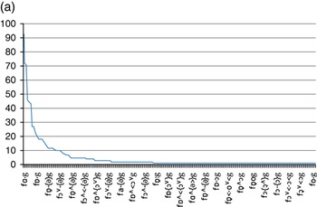
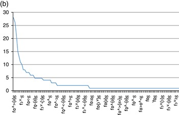
As shown in Figure 1 for realizations of the vowel in fog from the Middle and South Atlantic survey (called LAMSAS) of the American Linguistic Atlas, the order that emerges in speech when considered as a complex system is simply the frequency patterns of different possible variants, whether particular words, pronunciations, or constructions, that come to occur in the local communities, regional and social, and in the occasions for speech and writing, text types and registers, in which we actually communicate. A great many more variants per linguistic feature than we might imagine are in competition: LAMSAS field workers recorded 154 different phonetic strings to represent the fog vowel among the 1,162 speakers in the whole sample (see Kretzschmar, Reference Kretzschmar2010:275–276). While the differences in transcriptions are subtle, they represent how the highly-trained field workers were able to employ the IPA resources available to them. If we were to use acoustic phonetic methods (as illustrated in Kretzschmar, Kretzschmar & Brockman, 2013), we achieve similar results.

Realizations of fog in LAMSAS, overall vs. women only.

Of course the different regional and social and textual occasions overlap at different levels of scale, which makes speech inherently multidimensional, as shown here for the survey overall and for women. Even though the women are part of the overall sample, they commonly have more diphthongal pronunciations at high frequencies for this vowel than we observe in the whole sample, men and women together. The nonlinear shape of the frequency pattern is about the same at every scale and for every group (see Kretzschmar etal., Reference Kretzschmar, Kretzschmar and Brockman2013 for differences in curves at different scales), but different variants have different relative frequencies at different scales, as here. These frequency differences, the result of feedback in the complex system, differentiate the speech of different groups of people. The process at work in complex systems just explains better what we already knew: We tend to talk like the people nearby, either physically near or socially near, or both, and we tend to use the same linguistic tools that others do when we write or say the same kind of thing.
All speakers (n = 1162), top 20 responses
Chart (a) of 154 different responses Overall by frequency

Women speakers (n = 360), top 20 responses
Chart (b) of the 118 different Women's responses by frequency

Consideration of the complex system of speech, then, differs essentially from work on traditional models of diffusion. Rather than any hierarchical system of linguistic types in which entries change over time, what changes in a complex system is the frequency profile of a large number of variants. Rather than having a single value for a linguistic feature change from one state to another in any traditional model of diffusion, a binary change, the complex system of speech always has large numbers of competing variants which all change in frequency over time. Moreover, the scaling factor of complex systems accounts for the simultaneous coexistence of many varieties of the same language because the patterns of frequencies for different variants will be different for different populations, at the same time that we can describe the pattern of frequencies for population as a whole. Problems with description of the number of variants, as well as their frequencies at different times in different populations, no doubt help to create the contention discussed above between different traditional models for diffusion.
3. Introduction to Cellular Automata
As for diffusion in a complex system, as new variants of features arise, they compete with the many existing variants and may or may not come to be shared by an increasing number of speakers. As demonstrated by Nerbonne (Reference Nerbonne2010), the main factor in the process is proximity: Speakers have to be able to talk or write to each other in order for feedback and reinforcement to occur. The process of diffusion takes time, as reinforcement changes the frequency of the competing variants, and changes it differently in different places and groups and occasions for speech. We cannot observe diffusion directly because it happens too slowly and across too many speakers for us to watch, and in linguistics it has never been feasible to collect the time series data required to do so over stretches of time—imagine doing big surveys like the Linguistic Atlas or DARE or the Survey of English Dialects over and over and over again on an annual basis.2 We collect information at that rate and scale to chart the weather and the financial markets, but we may never do so for speech. Data gathered at one time, as from survey research, gives us a window on the state of the complex system of speech for one area at one time, for the frequency profiles for the linguistic variants sought for the survey. However useful that information is, it will never show the diffusion process itself in action. Computer simulation is the only way that we can model diffusion as the adaptive aspect of complex systems in speech and culture, so that we can watch it happen in one sitting.
To this end, the authors have built computer models, CAs, for use as a simulation for diffusion in a complex system. Holland, one of the fathers of computer modeling, has laid out its basic principles (Reference Holland1998): Define the state of the system, what operations may be performed by or on each of the components, and the conditions, or rules, under which an operation is performed. Running the model consists of starting with a given state and applying the rules to each of the components in one iteration of the model; then the rules are applied again for another iteration on the new state of the model; iterations of the model then can continue for as long as the states keep changing.
A CA is a particular kind of computer model (see Sarkar, Reference Sarkar2000 for a more mathematical survey of CAs than provided here). CAs can be constructed in one dimension, a line of locations, or in two dimensions as in our simulations, usually in a square matrix (more dimensions and other matrix types are possible but unusual; see Torrens & Benensen, Reference Torrens and Benenson2005, for examples). Given a starting state of the matrix, simple rules are applied at each iteration, the status of all the cells in the matrix is updated, and further iterations can then continue as long as need be. The concept of a CA was first introduced in the 1940s by Ulam and von Neumann (see von Neumann & Burks, Reference Von Neumann and Burks1966), but only received wider interest after Conway's Game of Life (GoL) simulation became available in the 1970s (Gardner, Reference Gardner1970). The GoL simulation is a simple CA in which each location in the matrix exists in one of two states (called “alive” or “dead”). GoL attempts to mimic the growth and change mechanisms of real-world dynamical systems, such as naturally occurring populations of the same species. The simulation has been studied as an entity of its own, but it—and CAs more generally— is also applicable to the study of other phenomena that can be modeled as systems consisting of individual actors following a common set of rules. CAs have been applied to the study of a multitude of physical, chemical, biological, and mathematical phenomena from river systems (Topa, Reference Topa2006) and traffic flows (Evans, Rajewsky & Speer, Reference Evans, Rajewsky and Speer1999) to the generation of random numbers (Tomassini, Sipper & Perrenoud, Reference Tomassini, Sipper and Perrenoud2000). Most CAs applied to physical phenomena in recent studies have been two-dimensional or three-dimensional in nature, and utilize rule sets more intricate than the rules of the GoL simulation.
CAs are generally classified according to their dimension and the type of patterns that appear during simulation. Wolfram (Reference Wolfram2002) famously carried out extensive experiments with one-dimensional CAs, and later terminology and concepts are based on this work. The patterns that CAs produce are generally classified into four groups following Wolfram's model (see also Sarkar, Reference Sarkar2000:94–96): 1) stable homogenity (e.g. all cells die), 2) oscillating structures (sometimes called “blinkers,” e.g. a blinking traffic light, or the three-light series of a normal traffic light, or sequential activation of cells around a wheel), 3) chaotic structures (e.g. random noise), and 4) complex structures (e.g. moving “gliders” in GoL, or complicated self-similar patterns). Of these types of patterns the last group has received the most attention when CAs are studied as an entity by themselves, but in real-world applications outcomes belonging to one of the other groups may also be valuable if they provide insight into the phenomenon under investigation. Group 1 patterns are easy to achieve with rules applied to sparse starting positions, or rules that allow adoption in most circumstances, and such outcomes are therefore usually viewed as uninteresting. For rules and starting positions leading to other patterns in the other groups, inhibition of uncontrolled growth is a major topic. In the GoL simulation this is addressed by specifying deterministic rules for both birth and survival conditions so that both birth and staying alive require enough neighbors to be present to overcome “loneliness” but having too many neighbors leads to death as a result of “overcrowding.” In more recent CAs similar behavioral control has been implemented via the introduction of a) cell memory of previous states, b) probabilistic rules, and c) rules that evolve over the generations of the CA. Alonso-Sanz and Margarita (Reference Alonso-Sanz and Margarita2003) provide an example of a one-dimensional CA where previous cell states affect the next state of a given cell. Factoring in past states causes a conservation effect that acts to confine any potential disruptions and also has the potential of transforming otherwise chaotic structures (Group 3) into stable or oscillating structures (Group 2) as the influence of memory is increased. Probabilistic rules can be used for the opposite goal of enabling disruptions by either allowing fully probabilistic cell states so that cells can be in several states at the same time, or simply to introduce a random factor to overturn rule decisions (Evans etal., Reference Evans, Rajewsky and Speer1999). Evolving rules may, for example, vary the birth and death requirements or the size and definition of neighborhoods (Mitchell, Crutchfield & Das, Reference Mitchell, Crutchfield and Das1996). CAs are inherently spatial in nature so it is not surprising that they have had applications in the study of phenomena where geography plays a significant part. Torrens and Benensen (Reference Torrens and Benenson2005) describe work on fusing a CA and a Multi-Agent System in order to create a CA with both fixed and non-fixed actors for use in urban simulations. This work is not unlike the work we present in this paper, although the system we propose takes a less mobile view of the actors.
In the social sciences, CAs have a long and continuous history of development. Two well-known foundational studies are Schelling (Reference Schelling1978) and Axelrod (2006), which used a CA to create, respectively, a dynamic model of segregation (how a racially-mixed population self-organizes into racially-similar housing clusters), and to demonstrate that “tit-for-tat” cooperation is the most successful strategy for social relations in the Prisoner's Dilemma game. So, for Schelling, each location became “black” or “white” according to update rules based on the current status of nearby locations, which altered the status of each location at each successive state of the matrix; over time clusters of black and white locations formed, which suggested how small differences in people's choices could lead to big differences in housing patterns. More recently, agent-based modeling has increased the number of dimensions for simulation over simpler CAs, so that update rules can apply to many characteristics for any location in a matrix, not just to a binary status like black or white; agents can also live and die, or change their locations. Gilbert and Troitzsch (Reference Gilbert and Troitzsch2005) and Gilbert (Reference Gilbert2008) provide a thorough introduction to agent-based modeling for the social sciences. Miller and Page (Reference Miller and Page2007) surveys principles of modeling as well as covering both CAs and agent-based models.
We are aware of only three earlier descriptions of CAs in language variation studies: Kretzschmar (Reference Kretzschmar1992) described the operation of a CA for the purpose of language diffusion studies; Keller (Reference Keller1994) reported unpublished work on an early cellular automaton that he compared to linguistic distributions; and Grieve, Speelman and Geeraerts (Reference Grieve, Speelman and Geeraerts2010) implemented a CA but without specific discussion of how its operation illustrated diffusion. Kretzschmar (Reference Kretzschmar1992) (the published version of a paper delivered in 1989) offered the rule-based process from CAs as an alternative to the subjectivity of drawing isoglosses; his experiments were not automated. Keller (Reference Keller1994:100–101; this is an English translation of his original book published in German reports the work of Levin from an otherwise unpublished 1988 mimeograph from the University of California-Riverside. Levin had created a small (55 × 55 cells) CA, in which he randomly seeded black and white cells. Keller reports Levin's rules as having the target cell stay the same if all of its neighbors had the same status, and that a white cell had a 51% chance of staying white if four of its neighbors were white and four were black. Keller offers a series of illustrations from Levin's CA that show how the random seeding, after many iterations, forms stable, coherent regions of black squares, and compared these regions to a map of dialect regions in Germany. Keller quotes Levin as saying that (1994:101)
I regard this as only a very primitive and abstract preliminary model that hopefully mimics linguistic interaction . . . Although my students became convinced that the grid was a territory, the squares villages or individual speakers, and the two variants [black or white squares] real language variants, I knew better.
Keller did quote Levin as saying that language change may “be understood on a grand scale as a kind of dynamic pattern emerging from simple and understandable interactive principles” (1994:101). We will return to this idea, now with greater justification from survey research and complex systems.
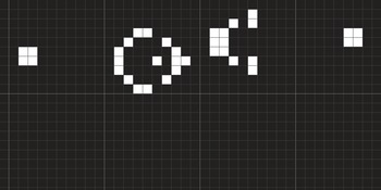
To offer a concrete illustration of the operation of a CA from the most famous CA, GoL (Gardner, Reference Gardner1970), if any black (or “dead”) cell is next to exactly three white cells, it becomes white (or “alive”); if any white cell is next to two or three other white cells, it stays white; in any other condition, the cell stays dark or becomes dark. These simple rules generate changes in iterations across successive time steps. When the starting position in Figure 2 is run with these rules, gliders continually form and appear to move across the matrix (this moving pattern is known as the Gosper Glider Gun). The application of rules constitutes exchange of information between cells, feedback, which then influences activity in the next iteration, reinforcement. CAs thus represent an appropriate method to model complex systems like speech.
Starting position for Conway's Game of Life (GoL) that generates “gliders.”

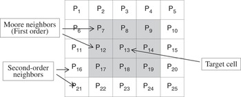
Just to be clear about what happens in a CA, Figure 3 is an illustration of a portion of a matrix (adapted from Mitchell Reference Mitchell2009: Fig. 14.4).
Moore neighborhood in a CA (adapted from Mitchell, Reference Mitchell2009).

The target location for the application of a rule is P13. The simulation looks at the first-order neighbors around the target to see how many are “alive” in order to see if the rule will make the target location either become “alive” or stay “alive.” In the Game of Life rules, P13 would have to have three of its gray neighbors, called the Moore neighborhood, be alive for it to become alive itself, or two or three live Moore neighbors to stay alive if P13 were already alive. It is also possible to consider second-order neighbors, but the usual practice in geography is to invoke the inverse square rule (not the same as a CA rule), which says that second order neighbors will have only 25% of the influence of immediate neighbors. Immediate proximity has the greatest effect. In sociolinguistics, Trudgill's Gravity Model for diffusion (Reference Trudgill1974) appears to break the proximity rule but actually it does not. Trudgill assumes that speakers from big cities have more contact with each other than with rural speakers in between, so he has substituted social proximity for geographical proximity and thus supports the idea that the most proximate speakers have the most influence on each other. As Nerbonne found, however, the effect of the Gravity Model is much less than the effect of immediate proximity.
4. Two Cellular Automata as Simulations
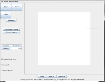
In our CAs we use the same basic tools--a matrix of cells, and simple rules to turn them on and off—but on a much larger scale than the earlier illustration of GoL. Our first CA, called GEM, has been programmed in Java by Bailey (Figure 4; GEM is available online at the journal site to download and use).
The GEM CA (screenshot).

Input rules for GEM are limited to the Moore neighborhood, i.e. to the eight cells immediately proximate to a target cell, and it is possible to select the number of neighbors required for the target cell to be “born” if it was dead, or to stay alive if it was already alive. The opening screen offers a 50 × 50 cell matrix, without living cells; the size of the “board” is adjustable, and it is possible to load maps. The user can draw (and save, if desired) a starting position of living cells, or generate a random starting pattern. It is also possible to draw “impassable” cells that are neither alive nor dead. These are useful for marking the borders of a region, or for creating barriers within a matrix, say to simulate mountains within a region.
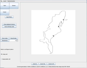
Figure 5 shows the boundaries of the LAMSAS survey region as they have been drawn with impassable cells, so that simulations can be run just within the survey area (this starting position is available online with the GEM CA). The board has also been expanded to 200 × 300, and living cells have been inserted near the locations of New York, Philadelphia, eastern Virginia, and Charleston, important colonial sites in America. Live cells in both of our CAs are black in color.
GEM with the LAMSAS region, living cells in four colonial sites (screenshot).

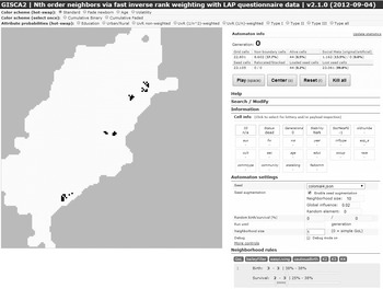
In our second CA, programmed in Javascript by Juuso and called GISCA2, the starting position includes 8,602 active cells, in the shape of the LAMSAS survey area (Figure 6).
The GISCA2 CA (screenshot).

The matrix is geocoded, so that each cell corresponds to a particular longitude and latitude and we can associate each cell with information we have about that location. Simulations begin with seeding of characteristics across the live cells of a large matrix, say, with a linguistic variant seeded along the coast to model original settlement. Here we start with just 44 live cells, where the Atlas interviewed speakers in Manhattan, Philadelphia, colonial Eastern Virginia, and Charleston, about one-half of one percent of the active cells in the matrix. Again, our live cells in both CAs are black in color. The borders of the LAMSAS survey region are buffered with additional live cells in GISCA2 to deal with what are called “edge effects,” and so our coastal locations appear to be a little bit inland.
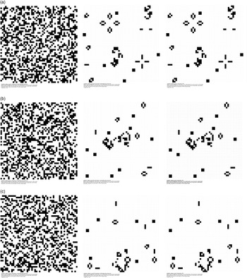
In order to be sure that our results from the two CAs came from the application of the rules we set, and not from differences in programming, we tested the programs against each other using the same starting positions and rule sets (Figure 7). The starting positions were randomly generated by GEM in a 50 × 50 matrix, and we applied the GoL rule set.
Three tests to validate equal performance of the two CAs (screenshot).

In each case we can see that the result after many iterations is exactly the same (i.e., if we overlay the two images, we will see no difference between the patterns of black squares). The experiment thus validates not only that it is the operation of the rules in these two CAs that create the final patterns, but that, in consequence, other properly programmed CAs will also be able to create the same patterns, given the same starting positions and rules. It is an important point to note that the computer does the same thing each time with a given starting position and rule set, and that the exchange of information that the computer executes on the CA is what is responsible for the pattern. When we get complex patterns from starting positions and rule sets, it is the interaction within the complex system that is responsible for the outcome.
4.1 Complex Systems and Cellular Automata
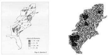
To return to speech, throughout hundreds of iterations that correspond to the daily interaction of speakers across time, we can observe distributional patterns as they emerge when speakers “adopt” or “maintain” a new linguistic variant. The key feature of this simulation, one not yet attempted to our knowledge, is that we also validate it with respect to the emergent “clustered” linguistic distributions known to occur in LAMSAS, not the actual patterns but instead the sort of pattern that emerges (Figure 8).
Clusters from real survey data and from the simulation.

We know that we have achieved a successful simulation of speech, not just a successful operation of a CA, if the result after hundreds of iterations is a complex system that shows the clustered distributions we expect in LAMSAS feature maps. As shown in Kretzschmar (Reference Kretzschmar2009), all LAMSAS distributions that we have measured tend to be clustered, as opposed to being regularly distributed, and of the features with moderate frequencies for which the statistic applies, fully three-quarters of the distributions are statistically significantly clustered. For example, at left we see a density estimation map of where LAMSAS speakers were likely to say chest of drawers, a feature studied extensively by Burkette (Reference Burkette2001, Reference Burkette2009). The map has clusters of places where the term is used more frequently than in the rest of the LAMSAS region, which represents the frequency profile we illustrated earlier for complex systems. At right, we see the output of a simulation that also has several clusters, not exactly the same ones as chest of drawers, but clusters, the dark patches, just like the ones from the real data. The point of our simulation, then, is a visualization. In the future we expect our simulations to achieve other parallels with LAMSAS data, like the regional and social nonlinear frequency distributions and scale-free networks that we always observe in our real data. We also expect to provide measures of clustering, and to explore the interaction of the length of time iterations are allowed to proceed and the degree of formation of clusters. However, for now we are satisfied with reproducing the appearance of the scattered clusters that we always see when we chart LAMSAS data.
4.2 Running the Simulation
As the simulation runs live and one watches the iterations (readers are invited to try the GEM simulation available online), the thing to see is that the map looks alive. What happens at any given location changes frequently, so that the whole map seems to flicker. It does not take many iterations for the target variant to occupy the rest of the area from the original seeds in colonial cities, as from the starting position in the illustrations above, but occupying the space does not mean that any of the locations permanently changes, becomes alive for good. Instead, the best characterization of what the simulation is telling us is constant motion. This kind of continuing activity does not arise as a consideration in traditional models of diffusion. Complex systems like speech, or like the human immune system, depend upon continuing interactions, this kind of constant motion, in order to adapt to circumstances and to allow the emergence of patterns appropriate to current conditions. A complex system is not a once-and-done process: If your immune system only created a set of antibodies once, you would not do well when you encountered a new pathogen. In language we must also adapt to new conditions, but our capacity to adapt to new circumstances also means that every part of our speech has to stay in motion like this, and so is subject to the emergence of new patterns. In a review of Kretzschmar's (Reference Kretzschmar2009) book, which focused on the nonlinear distributions and scaling properties discussed earlier, Larsen-Freeman (Reference Larsen-Freeman2011) asked where in the description of complex adaptive systems the adaptation was. This is it.
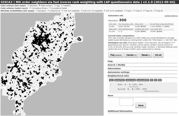
We can observe the motion of the system better with two advanced visualization tools built into the GISCA2 simulation. The first one fades out the new adoptions, so that we can see persistent patterns better, as shown in Figure 9 in a simulation stopped after 300 iterations (GEM has a similar tool that links age and opacity of cells). The cells that have only been alive for one generation are turned into a light grey color.
GISCA2 Fade tool for newborn cells (screenshot).

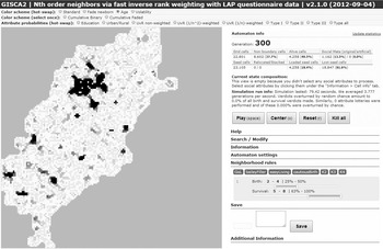
The visualization shows us two things. First, the simulation has a high number of such newborn, temporarily live locations, over 50% of the live locations, and a smaller number of patterns that stay alive over a longer time. We believe that this is intuitively similar to what happens in real speech, as speakers use many variants of constructions or pronunciations or words, perhaps on purpose but also by accident in the rapid stream of speech. This behavior accounts for the nonlinear pattern we always see, in which a few forms are very common but there is always a large number of infrequent forms. The second thing to see with the Fade tool is even clearer with the next visualization tool, an Age tool that colors locations by age so that we can see persistent patterns better. Figure 10 shows the same point in simulation, at 300 iterations, as in the previous figure. Cells that have been alive for 10% of the time of the longest living cell (e.g., for 12 generations if the longest living cell is 120 generations old) are colored black, with younger cells in shades of gray.
GISCA2 Age tool that shades cells by relative age (screenshot).

Like the temporarily live locations, most patterns are also not persistent. While many small clusters are formed, most of them disappear across the iterations. Even though this is the same state of the simulation, only a few of the black clusters remain from the visualization that fades only newborn cells. The visualization thus suggests that any patterns that might exist at one state at any given time will soon be gone. Some of the temporary patterns are moderately large and still completely fade away. Even the oldest patterns have gaps and constantly change at their edges. While the simulation does in the end produce persistent, stable patterns of locations that have been alive for a long time, which we can consider to parallel our perceptions of local and regional dialect areas (some of them of very long standing, such as modern British English dialect areas that occur in roughly the same areas as Anglo-Saxon kingdoms), we should understand just how rare these are, and how all patterns emerge from continuing activity within the complex system.
In our simulations we do not use the GoL rules, but instead a set of rules discovered by Bailey that we call the Bailey set or Bailey filler: A location in the matrix will adopt the target variant (become alive) if two, three, or four of its neighbors use the feature. A location in the matrix will maintain the variant when already alive if five, six, seven, or eight of its neighbors use the variant. The Bailey set is rare among possible rule sets. As documented by Wolfram for one-dimensional cellular automata and discussed above, rule sets may lead to four general categories of results. The first two are the most common but of little interest for speech: Rule sets that quickly result in a fixed state or a “blinking” state. Another kind of result is chaotic, in which locations just stay in motion turning on and off, and do not allow persistent patterns to emerge. This one also is not what we find in speech, where we do expect patterns to emerge. The last kind of result is what we want, the complex state that some have said is “at the edge of chaos” (Kauffman, Reference Kauffman1995). The Bailey set is the best one that we have found, one of only two or three possibilities for rule sets at the edge of chaos out of hundreds that we have tested in our two-dimensional CAs. We do not have enough information about the rules employed by Levin in 1988, as reported in Keller (Reference Keller1994), to assess how the Levin rules compare with the Bailey set.Footnote 3 Even the Bailey set is not enough by itself, as was apparently not the case for Levin's rules: After thousands of iterations it eventually produces one large cluster that fills the matrix. In order to slow down the progress towards one large cluster, in the GISCA2 CA we can include a random factor for overturning what the rules would have done. Speakers sometimes refuse to do what their neighbors do, just because they do not feel like it, and we have found that overturning the rules up to .06% of the time, six cases out of 10,000, slows down the unchecked expansion of clusters. Applying the random factor at .06%, though, keeps the Bailey set of rules from producing persistent clusters at all, because it appears to be the boundary for a transition to the chaotic result type. In the GEM CA, we can achieve a similar result by enabling random small-world neighbors, a few randomly chosen cells not in the Moore neighborhood for our target cell, but again the number of small-world neighbors selected will determine the result. So, slowly, across the iterations, we see that persistent clusters develop under the right conditions, though because of the random element even long-term clusters may in time disappear.
5. Conclusion
Our CAs, we believe, give us a successful simulation of diffusion. There is much more that we could say about the mechanics of CAs. Suffice it to say now that, in our work to date, we have demonstrated that stable clusters do emerge in the simulation as the result of restricted rule sets with a random component included. We have simulated the process of adaptation and diffusion, and we could not have done so without the foundation that the complex systems model provides. In contrast to work on traditional models of diffusion, our CAs show clearly how energetic interaction and feedback creates a dynamic adaptive system. Continual movement in the behavior of different locations, whether these are taken to be individuals or communities, certainly appears to be at the heart of diffusion, as we simulate change in operation. Of course, we have shown how diffusion works for only a single feature. Our future work will focus on the simultaneous diffusion of the variants of many features, so that it can help us to watch the emergence of the multidimensional scale-free network of speech that we perceive to be all around us every day. We do not believe that our simulations, or that our application of complex systems, argue against traditional models of linguistic diffusion, which clearly proceed from different assumptions. We do, however, believe that our simulations offer traditional studies of diffusion a new viewpoint from which to consider language change.
Supplementary Materials
To view supplementary material for this article, please visit http://dx.doi.org/10.1017/jlg.2014.2
Appendix
Directions for using the GEM Cellular Automaton
-
1. Download the GEM - Public.jar file and the two .json files, LAMSAS2CX3C.json and LAMSAS2CX3C-colonial4.json, from here (hyperlink to <http://dx.doi.org/10.1017/jlg.2014.2>).
-
2. You must have Java installed on your computer to run GEM. Most computers already have it these days. If you do not, go to http://java.com/en/download/index.jsp for a free copy, and install the program.
-
3. Double click on GEM – Public.jar to start the program. It should initiate and look like this

-
4. In order to load the LAMSAS map, click on File, then on Read Current State from JSON File. Navigate to the folder in which you downloaded the .json files, and select LAMSAS2CX3C-colonial4.json. Your screen should now look like this:
-
5. Click on the Input Rules box in order to select the rules you want. The default is the Bailey set of rules, 2, 3, and 4 for birth conditions, and 5, 6, 7, and 8 for life conditions. If you want to use the GoL set, click on 3 for birth conditions and 2 and 3 for life conditions. Of course, you can experiment with any rules you want to try.
-
6. Click the Start button to begin the simulation. You can make it go Faster or Slower with those buttons, and you can stop the simulation with the Stop button (in the same place as the Start button). If you want to save the state of the simulation, click the File tab and select Write Current State to JSON File.
-
7. You can clear the simulation and start over by clicking the Clear all living cells button. You must then use the cursor to draw in new seeds before hitting the Start button again: click the box for Living cell and click anywhere on the board to establish a living cell. You can also click the box for Impassable cell to make your own outline, like the outline of the LAMSAS region from the LAMSAS2CX3C-colonial4.json file; in addition, you could draw obstacles within an area to see how diffusion flows around them, say impassable cells in the LAMSAS region where there are mountains. Alternatively, if you click the Randomize button, it will randomly fill the matrix with cells up to the density you select (50 is the default). It will fill the whole matrix, not just the LAMSAS survey area. You can choose the Randomization method in Randomization tab at the top.
-
8. You may wish to try other options in the Board tab. If you click either the Link age and opacity box, or the Use small world neighbors box, a new setting box will open on screen for you to set the parameters you like.