

Published online by Cambridge University Press: 08 June 2005
This essay corrects the results reported in Gerber and Green 2000 and replies to Imai (2005). When data-processing errors are repaired, the original substantive findings from the New Haven experiment remain unchanged. As previously reported, brief phone calls do not increase voter turnout. The “correction” that Imai (2005) offers, which purports to show that these phone calls produce large, significant, and robust increases in voter turnout, is shown to contain statistical, computational, and reporting errors that invalidate its conclusions about the effectiveness and cost-effectiveness of phone calls and mail. A replication of the New Haven experiment reproduces both the findings reported in Gerber and Green 2000 and the biases of Imai's statistical analysis.
We are grateful to Kosuke Imai, who, in the course of replicating and extending our experimental analysis (Gerber and Green 2000), brought to our attention data-processing problems associated with our 1998 experiments on voter mobilization. However, the “correction” of our findings reported in Imai 2005 contains numerous statistical, computational, and reporting errors. The purpose of this essay is twofold: to offer a correction of our original findings and to demonstrate that the statistical analysis conducted by Professor Imai is systematically biased in favor of finding spurious effects.
The following section presents the corrected estimates from Gerber and Green 2000. The new version of the New Haven dataset shows no signs of randomization failure and generates statistical results that are substantively indistinguishable from what was reported in Gerber and Green 2000. Face-to-face visits increased turnout substantially; direct mail, modestly. Brief paid phone calls were ineffective. The section concludes with a replication of the New Haven study involving more than a million subjects. The results again show phone calls to be ineffective. The 6.5–percentage point effect claimed by Professor Imai (2005) is rejected at a significance level of less than one in a trillion.
The subsequent section explains why Professor Imai's statistical approach exaggerates the effectiveness of phone calls. We describe the faulty assumptions underlying his model and the nonstandard way in which he implemented propensity score matching. Replication of Professor Imai's (2005) analysis reveals a series of errors that call into question the magnitude, significance, and robustness of his matching estimates. This section concludes by showing that the biases of Professor Imai's matching analysis are not specific to the New Haven study; they can be reproduced using other experimental data.
Professor Imai raises a number of interesting and important methodological topics, ranging from research design to data analysis. However, this essay alerts readers to several instances in which Professor Imai's methodological advice is ungrounded in statistical theory and deviates from standard practice. The randomization check that he proposes produces incorrect p values and does not properly detect problems in the random assignment of experimental groups. His assurance that propensity score matching reliably estimates treatment effects is based on a dated and selective reading of the relevant literature, and at no point does he establish, analytically or empirically, the superiority of matching over other estimation methods, either in general or in this application. We show also that Professor Imai's advice about how to compare the cost-effectiveness of alternative get-out-the-vote tactics rests on an algebra mistake; using the correct formula confirms our original conclusions. His criticism of factorial design is groundless, both empirically and theoretically. His essay repeatedly points out the importance of assorted interactions and nonlinearities yet neglects to subject any of them to significance tests; doing so reveals that they are all insignificant. In sum, not one of the key substantive or methodological claims of Professor Imai's essay survives scrutiny.
Returning to the original data files, we reconstructed both the household-level and the individual-level New Haven study for purposes of preparing this correction. We corrected errors associated with (1) imperfect matches among names returned by the phone bank, names returned by canvassers, and names on the original master file, (2) a miscommunication between us and the phone bank about which treatment groups were to be assigned a get-out-the-vote appeal, and (3) data manipulation errors that caused some people in the control group to be incorrectly labeled as treatment subjects.1
The datasets that we prepared for Professor Imai in June 2002 addressed problems 2 and 3. The correction to problem 3 accounts for the change in the number of treatment group observations from 958 to 805 in his Tables 1 and 2 and explains the slight increase in the contact rate reported in his Table 4. Problem 1 did not become apparent until a year later, when, with the assistance of a database programmer, we reconstructed the dataset from the four original data files (the master file of treatment assignments, the names and contact information reported by the phone bank, vote histories, and results from the door-to-door canvass). This process also corrected errors in the party and age variables.
Before analyzing the data, we first demonstrate that nothing is amiss in the random assignment of subjects to treatment groups. Since the data were randomized at the level of the household, this randomization check must also be performed at the household level (N=23, 450). Performing the randomization check at the individual level, as Professor Imai does (his Table 6), provides grossly misleading results because individuals living in the same household share the same background characteristics, such as voting ward. Monte Carlo simulations reported by Arceneaux, Gerber, and Green (2004) demonstrate that even when the household-level assignments to mail, phone calls, and visits are generated at random, estimating the randomization check at the individual level incorrectly declares one or more of these randomizations flawed in more than 95% of the simulated experiments. Professor Imai cites McCullagh and Nelder (1989, 119) as an authority for his test, but they warn (118, assumption 1) that their result hinges on the assumption that the observations are independent. Due to this error, all of the p-values reported in his Table 6 are incorrect.
Using logistic regression, we regressed each experimental assignment—mail, phone, and face-to-face canvassing—on all of the background information available for each household: the ward of residence, the number of voters in the household, the age of each voter, a dummy variable for missing age information, dummies indicating whether each voter abstained in 1996, dummies indicating whether each voter voted in 1996 (the omitted category was not being on the voter rolls in 1996), and dummies indicating whether each voter was registered with one of the two major parties. This exercise generates chi-square statistics with 39 degrees of freedom. We do not follow Professor Imai's procedure of including more than 100 first-order interactions among these variables.2
In his footnote 18, Professor Imai (2003) advocates the use of even more interactions and higher-order terms than he was able to implement in this application. For an example of a properly conducted randomization check, see Ansolabehere and Iyengar 1995, 172.
Applying the proper randomization check to these data reveals that the p-values from these regressions are nonsignificant: .95 for mail, .78 for phone, and .39 for face-to-face canvassing. A superior way to assess randomization is to analyze assignment to all eight experimental permutations simultaneously. A multinomial logistic regression with 273 degrees of freedom produces a nonsignificant χ2 of 261 (p=.70). (Employing Professor Imai's method of including all first-order interactions raises the number of degrees of freedom to 1,764 and decreases the p-value to .27.) After deleting households that did not have valid voting data in 1998, we obtain similar results (N=22, 449); the p-value for mail is .93; phone, .76; and face-to-face canvassing, .43. The multinomial regression produces a p-value of .60.3
Nonsignificant p-values are also obtained for all the subsamples that Professor Imai analyzes: p=.54 when excluding households that received multiple treatments and p=.66 when further excluding households that received a placebo phone call asking for a blood donation.
Professor Imai (2005, 290) concedes that two-stage least-squares (2SLS) is the best estimator for gauging treatment effects when the treatments are assigned at random. This estimator is the multivariate generalization of the instrumental variables estimator proposed by Angrist, Imbens, and Rubin (1996). The vote is regressed on actual treatment using treatment assignment as an instrumental variable (see Statistical Implications of Failure to Treat, below). The next section applies this estimator to the corrected experimental data.
Using the corrected individual-level data, Table 1 reports the 2SLS regression estimates. Looking first at the model without covariates, we see that the estimated effect of face-to-face canvassing changes from 8.7 (published) to 8.4 (corrected). Mail's effect changes from 0.58 (published) to 0.51 (corrected). The coefficient estimate for phone calls remains negative. The published value of −4.7 is corrected to be −1.9. A similar pattern holds when we estimate the treatment effects controlling for voting history, age, party registration, and ward of residence. Again, the published estimates change from 9.8 to 9.0 (face-to-face canvassing), from 0.63 to 0.59 (mail), and from −3.5 to −1.7 (phone). The inclusion of covariates reduces the standard errors slightly but otherwise has little effect on the results.
Correcting the coding errors in the New Haven study changes none of the substantive conclusions that flow from it. Door-to-door canvassing's effects are large and statistically significant using a one-tailed test. Mail's effects are small and borderline significant using a one-tailed test. Phone's estimates are negative and, of course, not significantly greater than zero using a one-tailed test.
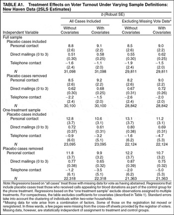
The results do not change when one discards the experiment's factorial design. Professor Imai sharply criticizes factorial designs, referring to them in the text and tables as “incorrect.” (This usage has the unfortunate consequence of creating confusion between our data-processing errors and the supposed “error” of assigning observations to multiple treatments.) His approach is to throw out all observations that were assigned to more than one type of voter mobilization treatment. We have more to say about this practice below. For the moment, note that the estimated effects of the phone treatment do not change substantively when one restricts the sample to this subset of observations, although the standard errors grow considerably because the N in the phone treatment group (excluding those assigned to the placebo condition) drops from 6,562 to 815. The phone treatment effect becomes −2.0 (SE=6.2); with covariates, the estimate is −5.0 (SE=5.3). Professor Imai leaves the impression that the negative estimates produced by the New Haven study reflect randomization failures or the misguided use of a factorial design. It is now clear that the negative estimates have nothing to do with randomization failure or use of multiple treatments. Table A1 (Appendix) shows that, regardless of sample definition or model specification, all of the models produce negative estimates. Some estimates are more negative than the results reported in Gerber and Green 2000.
What substantive inference do we draw from these negative estimates? Notwithstanding the title Professor Imai selected for his essay, at no point did we assert that get-out-the-vote phone calls reduce turnout. What we said (Gerber and Green 2000, 660) was, “Given our initial expectation that telephoning increases turnout, we take this to mean that the null hypothesis of no effect cannot be rejected using a one-tailed test.”4
Professor Imai relegates a fragment of this quotation to a footnote and inserts into his text a quotation from a paper on a different experiment published in another journal (Gerber and Green 2001). He quotes from a footnote in the 2001 article, where, after finding insignificant negative coefficients, we offer a speculation about why the commercial phone bank “conceivably” could have had a negative effect. The text of Gerber and Green 2001 (cf. 76, 80, 81, 82) leaves no ambiguity about our interpretation. We observed that “phone canvassing did not seem to affect voter turnout in our experiment” and that “get-out-the-vote calls produced no statistically significant increase in voting rates.”
Gerber and Green (2000, 660) describe the negative effect of get-out-the-vote calls as “one of the most surprising results to emerge from our experiment.”
We also conducted a replication study of sufficient size to potentially refute our earlier conclusions. This study was designed to be above complaints about factorial designs or the inclusion of multiple individuals from the same household. Two national phone banks read a script much like the ones used in the 1998 study.5
The script read: “Hello, may I speak with [name of person] please? Hi. This is [caller's name] calling from Vote 2002, a non-partisan effort working to encourage citizens to vote. We just wanted to remind you that elections are being held this Tuesday. The success of our democracy depends on whether we exercise our right to vote or not, so we hope you'll come out and vote this Tuesday. Can I count on you to vote next Tuesday?”
The populations used for this study were registered voters in Iowa and Michigan. These states were chosen because they maintain high-quality computerized voter files with the vote history of each registered voter. We use this information later, when we apply matching to these data. The congressional districts of each state were divided into “competitive” and “uncompetitive” strata. Within each stratum, households containing one or two registered voters were randomly assigned to treatment and control groups.6
As a randomization check, we used logistic regression to predict treatment based on vote in 2000, age, number of registered voters in a household, and state house district. As expected, the chi-squares for each stratum are nonsignificant: Iowa noncompetitive (df=24, p=.49), Iowa competitive (df=63, p=.72), Michigan noncompetitive (df=95, p=.60), and Michigan competitive (df=31, p=.23).
Given the enormous sample size, the experiment can easily detect the 6.5–percentage point effect that Professor Imai reports in his Table 9. The 2002 results, however, closely resemble our 1998 findings. The effect of the treatment-on-the-treated, controlling for the design strata (competitiveness levels within each state), is 0.4 percentage point.7
The effects of phone banks are similar across states (Iowa, b=0.6, SE=0.6; Michigan, b=0.1, SE=0.8), competitiveness strata (uncompetitive districts, b=1.0, SE=0.7; competitive districts, b=−0.3, SE=0.7), and commercial phone bank firms (first phone bank, b=0.6, SE=0.9; second phone bank, b=0.2, SE=0.6). The results remain unchanged when controls are introduced for past voting behavior and age (b=0.4, SE=0.4).
The experiments just summarized do not mean that all forms of phone canvassing are doomed to fail. As we stated (Gerber and Green 2000, 661), these findings demonstrate only that brief, mechanically delivered reminders to vote conducted by commercial phone banks have negligible effects on voter turnout. In subsequent research, we studied alternative phoning strategies to see how phone banking might be conducted more effectively. In Green and Gerber 2001, we drew the distinction between the commercial phone banks studied in Gerber and Green 2000, 2001 and volunteer phone banks delivering chatty, informal scripts. Ignoring this distinction (which is spelled out explicitly in the second paragraph), Professor Imai (2005, 298) cites this report as evidence that his “correction” squares with other results showing that phone banks increase turnout significantly. The thesis of Gerber and Green 2000 is not that door-to-door canvassing invariably works while phone calls invariably fail; it is that the effectiveness of alternative forms of voter mobilization increases when messages are delivered in an authentic, personal manner.
Professor Imai's central substantive claim is that we have overestimated the cost-effectiveness of personal visits vis-à-vis phone calls and direct mail. The experimental studies cited above show that calls from commercial phone banks have negligible effects on voter turnout. If four votes are produced for each 1000 people who are contacted by a commercial phone bank and if one pays 50 cents per contacted person, each additional vote costs $125. Commercial phone banks delivering brief nonpartisan get-out-the-vote calls are clearly not a cost-effective way to increase voter turnout (see Cardy 2005 and McNulty 2005 for similar findings regarding partisan calls from commercial phone banks). Let us now turn to Professor Imai's further claims concerning direct mail.
Professor Imai (2005, 290) contends that we have “underestimated the effectiveness of sending postcards by incorrectly comparing the estimated ITT [intent-to-treat] effects for postcards with the estimated treatment effects for visits.”8
See below for a discussion of ITT effects.
To calculate the cost per vote of a mailing regimen, we reasoned as follows (Gerber and Green 2000, 661): “At fifty cents per mailer, sending three mailings to each household (containing an average of 1.5 voters) nets roughly one additional voter per $40 spent.” This figure was calculated based on our two-stage probit estimates using the following formula:

Using propensity score matching, Professor Imai reports in his Table 9 that three mailings increase turnout by 1.5 percentage points (SE=1.0). This statistically insignificant estimate implies a cost-per-vote estimate that is even higher than ours: $1.50/(1.5×0.015)=$66.67.
Next, we take up the charge that our comparison of the relative effectiveness of mail and visits is miscalculated. Here is how we calculated the cost-effectiveness of visits (Gerber and Green 2000, 661): “Similar calculations, using $1.50 as the cost per personal contact (10 contacts per hour at $15 per hour), produce an estimate of approximately one more voter for each $8 spent.” Expressed algebraically, that calculation looks like this:

Professor Imai's matching estimate of 9.2 percentage points (see his Table 9) generates a cost-per-vote estimate of $10.87 for personal visits. Either way, personal visits are more cost-effective than direct mail.
These calculations produce the same answers if we use ITT estimates and rescale the calculation to eliminate contact rates. Let Ca be the cost per attempted treatment, and let Ta be the number of votes produced per attempted treatment. The cost per vote of this intervention may be calculated as Ca/Ta. If, instead, we define Cr to be the cost of actually contacting someone, Cr is equal to Ca (the cost of attempting to treat) divided by α (the proportion of people in the treatment group who are actually treated). The number of votes produced per actual treatment is Tr, which equals Ta/α, since the treatment-on-treated effect is the intent-to-treat effect divided by the contact rate. It follows, therefore, that cost per vote equals

This equation refutes Professor Imai's (2005, 290) assertion that it is “inconsistent” to calculate cost per vote using treatment effects for visits and ITT effects for mail. Suppose we take Professor Imai's advice to allow for the fact that some people do not read their mail. That means dividing both the numerator and the denominator by α, which leaves the estimated cost-efficiency unchanged.9
For example, if one believes that only one-fourth of those who were sent mail read it, the treatment-on-treated effect for mail would be four times greater than the ITT effect. However, the cost per actual treatment would also be four times higher than the cost per attempted treatment.
The experimental evidence leaves little doubt about whether brief nonpartisan phone calls from telemarketing firms are effective. The remaining question is why Professor Imai's matching analysis produced inaccurate estimates. This section traces the bias in Professor Imai's estimator to two sources, the assumptions underlying the method and the problematic way in which it was implemented and reported. First, we model the selection problem that this matching procedure purports to solve. Second, we note several instances in which Professor Imai exaggerates the inadequacies of instrumental variables estimation as a method for analyzing experimental data. Third, we show that the matching estimator that he offers as an alternative relies on much stronger substantive assumptions. Fourth, a review of the matching literature reveals that the general properties Professor Imai ascribes to this method are not supported by the empirical track record of this technique. Fifth, we show that the evidence that Professor Imai marshals to demonstrate the significance and robustness of his estimates is marred by computational errors and discrepancies between the results of his computer programs and what he reports. When these defects are corrected, it turns out that his method fails both of the specification tests that he proposes as ways of detecting bias in propensity score matching, as well as two further specification tests that follow from the logic of his model. Finally, we demonstrate that the biases of Professor Imai's estimator are not specific to the New Haven study. Applying matching to the replication experiments conducted in 2002 shows that this estimator again severely overestimates the effects of brief nonpartisan phone calls.
When estimating experimental treatment effects, analysts must attend to complications that arise when some of the people who are assigned to the treatment are not actually treated. In the case of the New Haven experiment, for example, 32% of the 5,275 households assigned to receive get-out-the-vote phone calls in fact received them. The remaining 68% had unknown or nonworking telephone numbers, never answered the phone, or hung up on callers before they could read their scripts. Failure to treat a portion of the assigned treatment group creates a selection problem: if those reached by phone have a greater propensity to vote than those who were not, a comparison of the treated group (those actually reached by phone) and the control group will overstate the effects of phone calls. Even if the phone calls truly have no effect on turnout, they may appear to have large effects.
In Gerber and Green 2000, we presented a model of the selection process and used it to derive an estimator of the treatment effect that is consistent even in the presence of this selection problem. Suppose that for a given canvassing effort, the population can be divided into two groups, those who are reachable and those who are not. Let α be the proportion of the population that is reachable. Let
be the probability that a nonreachable person votes. Let pr be the probability that a reachable person votes in the absence of an experimental treatment, and let pr+t be the probability that a reachable person votes after exposure to the experimental treatment.10
The parameter t can vary across those contacted, in which case t is interpreted as the average treatment effect among those actually treated.
In the control group, we do not observe who is reachable and who is not. What we observe is the voting rate for the group as a whole. The expected voting rate in the control group (PC) is

When treatment and control groups are formed randomly, both groups have the same expected proportions of reachable and nonreachable people. In this case, the expected voting rate in the treatment group is

Manipulating these equations and solving for t suggests the instrumental variables (IV) estimator for the treatment effect:

The numerator of this equation is the estimated ITT effect: it is simply the difference between the voting rate in the assigned treatment group (the subjects the experimenter intended to treat) and the voting rate in the control group. The denominator contains the “contact rate”: the fraction of people in the treatment group who were actually treated. Both quantities are easily calculated from experimental data. Because the contact rate is positive, ITT and t always share the same sign. We show below that Professor Imai's matching analysis does not satisfy this logical requirement. When analyzing the effects of phone calls, matching generates a negative estimate of the ITT but a positive estimate of the treatment effect.
Professor Imai concedes that when experimental groups are assigned randomly, IV is the appropriate estimator of the treatment-on-treated effect (often referred to as simply the “treatment effect”). He argues that when groups are not assigned randomly, the IV estimator generates biased results. This argument is moot with respect to the experimental evidence presented above; the updated version of the New Haven dataset, as well as the Iowa and Michigan replication studies, shows no signs of randomization problems. This is not the only concern that Professor Imai raises about IV, however. To justify matching, Professor Imai advances a number of additional criticisms of IV estimation. These criticisms rest on three flawed arguments.
Professor Imai (2005) writes that it is “important to note” the finite sample bias of IV estimation and claims that the small size of our treatment groups “suggests the importance of finite sample considerations” (his footnote 18). However, the “importance” of small sample bias in our particular case is merely an assertion. It is easy to assess the small sample bias, under various contact rates, using simulation methods. Doing so reveals Professor Imai's concerns to be groundless (for Monte Carlo results, see Gerber and Green 2004b).
In his footnote 18, Professor Imai contends that IV is “inefficient” and cites Bound, Jaeger, and Baker (1995) for support. Bound et al. make no such claim. This appears to be one of several instances where the term of art “inefficient” is misused as a synonym for “large standard error.” Professor Imai attempts to bolster this theoretical claim with evidence, repeatedly assailing the IV estimator on the grounds that its estimates are sometimes positive and sometimes negative when applied to the New Haven study. This line of argumentation conflates the properties of estimators (algorithms) with the behavior of estimates (statistics obtained from a particular sample). Professor Imai fails to explain that the apparent volatility of his IV estimates stems not from the properties of the IV estimator but rather from the simple fact that he restricts his attention to small subsamples of the New Haven data. To produce the astonishing −27 estimate that he twice mentions on the first page of his article, Professor Imai takes the subjects who were assigned to the phone treatment, discards those who were also assigned to receive mail or visits, and then discards those who reside in households with two registered voters. That leaves 7% of the original treatment group. It is hardly surprising that dramatic reductions in sample size increase the volatility of the IV estimates.
In the model presented above, randomization ensures that both the treatment and the control groups have the same expected proportions (α) of reachable and nonreachable people. In any given dataset, these proportions may differ due to sampling error. Professor Imai's discussion of randomization frequently confuses the properties of randomization as a procedure with the outcome that results from a given random assignment. Randomization is an unbiased procedure even if in a particular experiment it produces a treatment group with too many young people or too many people in a certain section of town. To the extent that randomization generates observable differences between treatment and control groups, an appropriate corrective is to control for these differences. For this reason, Gerber and Green 2000 reports the experimental estimates both with and without controls for background characteristics. This point is glossed over in the “replication” tables presented in Imai 2005, which exclude covariates.
How is the IV estimator affected when randomization is compromised by clerical error? Suppose that certain subjects had a greater probability of being assigned to the treatment group. This failing is not a sufficient cause of bias. Bias results only when the experimental assignment is correlated with omitted causes of the vote. Thus, even if Professor Imai had obtained significant results from a properly performed randomization check, he would not have established that the systematic patterns in the experimental assignment produced biased estimates. Professor Imai attempts to fill this logical gap by demonstrating that the treatment and control groups have different propensities to vote. He reports that in select subsamples, there are small and marginally significant correlations with past voting (Imai 2005, 293). Professor Imai neglects to mention that none of the treatment groups (phone, mail, or visit) bears a significant relationship to past voting in the sample as a whole. Nor are the treatment assignments correlated with age, number of voters in the household, or party registration. The largest absolute correlation between the phone treatment and any of these variables is .01 (nonsignificant), and jointly they do not significantly predict any treatment assignment in a logistic regression. It is not surprising, therefore, that correcting the clerical errors in the original New Haven data had little effect on the results.
We now turn our attention to propensity score matching, which Professor Imai represents as a superior statistical method.
IV compares the turnout rates of those assigned to the treatment group with the turnout rates of those assigned to the control group, because these groups have been formed in a way that ensures their comparability. The point of performing randomized experiments is to liberate analysts from making strong assumptions about the unknown values of pr and
.
Professor Imai's matching analysis, by contrast, compares those who actually received the treatment to the control group, after controlling for background characteristics. (This type of comparison has been shown to produce biased estimates in fields such as biostatistics; see Lee, Ellenberg, Hirtz, and Nelson 1991.) Suppose one were to restrict the sample to subjects who share exactly the same background characteristics, such as age, party, and voting history. For this subgroup, Imai's estimator may be expressed as

The last term in this equation represents the bias in the matching estimator. When
, this last term cancels, and the bias is zero. In other words, the matching approach will work if, after controlling for background characteristics, reachable and nonreachable people become interchangeable. This is a very strong (and demonstrably false) assumption. Bear in mind that in the version of the New Haven data that Professor Imai analyzed, the voting rate among those reached by phone was 64.8%, compared to 44.4% among those in the control group. By controlling for background characteristics, Professor Imai whittles this 20.4–percentage point gap down to 6.5 percentage points. The question is whether the background information that he used was sufficient to control for all of the unobserved factors that could account for higher voting rates among those who answered the phone. The experimental results as well as the specification tests presented below demonstrate that the answer is no.
Because Professor Imai's estimator compares those actually treated to a comparison group of untreated individuals, it must overcome a selection problem. Although he declares that “when treatment assignment is not completely random and important covariates are observed, propensity score matching is the best available statistical method” (295), his enthusiasm is not shared even by authors of the articles that he cites. Heckman et al. (1998, 1019), for example, caution:
In general, matching is not guaranteed to reduce bias and may increase it…. Moreover, matching is open to many of the same criticisms that have been directed against traditional econometric estimators because the method relies on arbitrary assumptions. Even with the rich data at our disposal, the method of matching is not, in general, an effective evaluation method.
Propensity score matching's mixed record is not reflected in Professor Imai's essay. He does not cite a single work on propensity scores written by others in the past six years, with the lone exception of Dehija and Wahba (1999). Professor Imai (2005) cites this article to bolster the claim that “matching is known to effectively reduce bias caused by nonrandom treatment” (295) but neglects to report a well-known critique of their work, which claims that Dehija and Wahba's results were an artifact of questionable sample restrictions and faulty analysis (Smith and Todd 2001).
Are there any special reasons why propensity score matching is particularly well suited to gauging the effects of voter mobilization campaigns in the New Haven study? Professor Imai (2005, 295) offers three reasons to believe so:
First, since the large control group roughly represents the population, we know that potential compliers exist in this group. Second, as shown later, I find many exact and close matches, indicating that the bias due to inexact matches is minimal. Third, when the covariates measuring important characteristics of the subjects are available, propensity score matching is a powerful method for reducing bias.
Professor Imai's second argument avoids the central issue, which is the possibility that individuals who are successfully treated are different from individuals in the control group who share the same background characteristics. This argument also turns out to be misleading since the matching estimates reported in his Table 9 for the phone treatment are not based on exact matching. When estimating the effects of phone calls, Professor Imai matches each person who received a call to five people in the control group with the nearest propensity scores. Only a small proportion of these matches is exact. As we show below, the problem of inexact matches contributes to the bias in Professor Imai's estimates.
Professor Imai's third argument repeats his unsupported assertion about the power of matching to reduce bias in general. The analytic and empirical literatures on the subject give no such assurances about the general properties of the method.
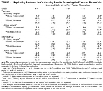
Table 2 shows that Professor Imai also exaggerates the magnitude, significance, and robustness of his matching estimates. We summarize four errors in Professor Imai's text and tables; interested readers may replicate these results for themselves using the replication programs we posted.
Bootstrapping is “a tool for developing inferential statistics (i.e., confidence intervals and bias estimators), not point estimators of parameters” (Mooney and Duval 1993, 60). The point estimates that Professor Imai reports in his Table 9, however, were obtained by drawing N observations with replacement from the actual sample and then averaging over 500 replications of this procedure. This bootstrapping procedure generates distorted results. Table 2 compares bootstrapped estimates with estimates from the actual sample. The estimated effects of phone calls fall to insignificance when based on the actual sample. His matching program generates an estimate of 5.1 (SE=3.3) when performing one-to-five matching on the actual sample, and this number drops to 3.6 (SE=4.5) when one-to-five matching is performed with replacement.
Table 9 of Imai 2005 exaggerates the significance of the phone effect by reporting a coefficient of 6.5 with a standard error of 3.2. These numbers imply a t-ratio of 2.03, which tells the reader at a glance that the effect is statistically significant using a two-sided test (p<.05). When these numbers are replicated using 500,000 bootstrap samples rather than 500, the correct estimate is 6.2, with a t-ratio of 1.87 (see Table 2). When we repeated Professor Imai's procedure of 500 bootstrap samples 1,000 times, only 2% of the time did we obtain a t-ratio as high as 2.03.
Professor Imai describes two sensitivity tests for his implementation of one-to-five matching. The first test indicates that the results do not depend on whether one performs one-to-five matching or one-to-one matching. Acknowledging that one-to-many matching causes the match quality to deteriorate, Professor Imai (2005, 299) notes, “If the results based on one-to-many matching are significantly different from those of one-to-one matching … we may conclude that the former suffers from large bias.” His Table 9 indicates that one-to-five matching produces an estimate of 6.5; his text reports that one-to-one matching generates an estimate of “six” (299). This is incorrect. The one-to-one matching estimate is in fact 4.3, with a standard error of 4.1. Moreover, as the first row in Table 2 indicates, there is a clear relationship between the number of matches and the size of the estimated treatment effect: the greater the number of matches, the larger the estimated effect. The second sensitivity test is found in Professor Imai's footnote 24: “I report the results for matching without replacement, but the sensitivity analysis using matching with replacement produced similar results.” The exact numbers behind these “similar results” are not reported. We report them in Table 2. Using Professor Imai's program, we find that the bootstrap estimate for one-to-five matching with replacement is 4.0 (SE=4.5). For one-to-one matching, the figure is 3.7 (SE=4.8). These numbers convey a different impression of the treatment effect from the estimate of 6.5 (SE=3.2) reported in his Table 9.
A recurrent theme of Professor Imai's paper is the superior performance of matching when applied to subsamples of the New Haven data, such as those living in households with either one or two registered voters. His argument is that a good estimator produces similar results across subgroups.11
This hypothesis shifted over successive versions of Professor Imai's APSR article. Professor Imai (2002, 25) earlier predicted a larger effect for one-voter households. The matching estimates reported in that paper supported his prediction.
When reporting the corrected results, we have followed Professor Imai's practice of dividing the sample according to whether the treated subjects live in one- or two-person households. Professor Imai's program matches these subjects to the nearest propensity scores in the control group, regardless of whether these control subjects reside in one- or two-person households. He does not alert the reader to this fact, which invalidates the comparison between matching and IV for one- and two-voter subgroups. The computer error does not affect his estimates for mail. Without explanation, he estimated these matching models separately for one- and two-person households.
Two important errors of omission must also be mentioned. The first concerns the negative ITT effects of phone calls. Logically, the effect of assigning people to be called must be the same sign as the effect of actually calling them. Although Professor Imai reports the ITT estimates using regression and claims that ITT estimates are needed for cost-effectiveness comparisons, he reports the matching estimates of the ITT effect only for mail, not for phone calls. Instead, the reader is shown only the positive matching estimates for the phone treatment effects and is informed that the negative estimates generated by OLS and 2SLS somehow reflect the deficiencies of these estimators when applied to flawed experimental data. Table 2 shows that the negative ITT estimates have nothing to do with the use of linear, parametric estimators. Using Professor Imai's matching program, we estimated the ITT effect of phone calls. Regardless of the number of matches and regardless of whether one uses the actual sample or bootstrap samples, propensity score matching always produces insignificant negative ITT estimates, ranging from −2.8 to −2.1, with standard errors ranging from 1.9 to 2.6. (Bowers and Hansen 2005, analyzing the same data, also obtain weakly negative ITT estimates using matching.) The implication is that the effects of phone calls were statistically indistinguishable from zero.
The second omission is the failure to check whether the nontreated vote at the same rate as the control group. The key identifying assumption in Professor Imai's estimator is that the people who are reached by phone (the “treated” group) are identical to the people in the control group who share background characteristics. This reasoning leads him to infer the causal effect of phone calls from the fact that these two groups vote at different rates. Looking only at Professor Imai's results, one cannot know whether the observed differences between the treated group and the matched control group reflect a true positive effect of the treatment or the upward bias of the matching procedure (see Eq. [4] above). But the same logic also implies that people who were assigned to the treatment group but not contacted will vote at the same rate as those in the control group with similar background characteristics (see Imai 2005, Figure 1). Since there can be no treatment effect without a treatment, the difference between the untreated and their matched counterparts can only be attributed to the bias of the matching estimator.
Using Professor Imai's matching program to compare the noncontacted members of the treatment group to the control group reveals that those who could not be reached by phone vote at substantially lower rates. The estimate produced by one-to-five propensity score matching is −5.6, with a standard error of 2.3.13
The propensity score model used to generate this estimate uses all of the main effects and first-order interactions among the background variables. This model passes the balancing tests described by Professor Imai.
The remaining question is whether the pattern of biases detected in the New Haven data can be reproduced in other studies. The answer is yes. When we apply matching to the enormous Iowa and Michigan samples, using covariates similar to those available in the New Haven study, we obtain upwardly biased estimates of 4.2 (SE=0.4) and 3.2 (SE=0.5), respectively, for the effects of phone calls.14
The large sample sizes of these studies enable us to use exact matching, rather than propensity score matching (see Rosenbaum and Rubin 1985 on the superiority of exact matching). Because the treated and control observations share exactly the same values of the covariates, the two groups are automatically “balanced.” In Iowa, 10,299 of the treated observations (75%) were matched to 132,577 observations in the control group. In Michigan, 9,565 of the treated (85%) were matched to 167,599 observations in the control group. To mimic the New Haven study, the control groups in Iowa and Michigan included randomly selected individuals without known telephone numbers.
Professor Imai contends that, when properly analyzed, the New Haven experiment shows that phone calls dramatically increase voter turnout. Due to the ready availability of experimental data, Professor Imai's conclusion can be evaluated with rare precision. The New Haven experiment and other large-scale field experiments demonstrate the ineffectiveness of brief calls from commercial phone banks. The probability that the treatment effect is as large as the 6.5 that Professor Imai presents is effectively zero.
Having addressed Professor Imai's main statistical claim, we conclude by briefly responding to three further criticisms that he levies against the analysis presented in Gerber and Green 2000. These criticisms allege that (1) the use of factorial design in the New Haven experiment was “incorrect” and “inefficient,” (2) we failed to take notice of many important nonlinearities and interactions, and (3) we resist the use of advanced statistical methods.
Professor Imai (287–288) sharply criticizes the use of factorial design and declares the use of multiple treatments “incorrect” and “inefficient.” Asserting that “in principle, it is advisable to minimize the number of treatments in field experiments” (288), his correction to the New Haven study is to discard all observations assigned to multiple treatments (289). We would caution readers that Professor Imai's practice of discarding all observations assigned to multiple treatments is highly idiosyncratic. He cites no authorities, provides no statistical analysis, and ignores the large and trenchant literature that endorses factorial design, particularly in the early phases of a research program (see Mead 1988, 584–85).
Professor Imai's discussion of factorial design is predicated on a mistaken understanding of what it means to estimate the “marginal effect” of a treatment. This endeavor does not require one to compare a single treatment to a pure control group. On the contrary, a marginal effect refers to a change from one experimental condition to another, holding other factors constant. For example, to estimate the marginal effect of a visit, we might compare those who were assigned only visits to those who were assigned nothing. But we might also look at those who received visits and mail to those who received only mail. The latter simulates the effects of visits in a campaign environment in which voters are receiving mail. Neither can be deemed “correct” unless one stipulates that only certain kinds of campaign environments are worth studying. To characterize the design of the New Haven study as “inefficient” because it did not focus on just a single type of marginal effect fails to appreciate the aims of the experiment, which sought to explore treatment effects across a range of different conditions. And to denounce the use of factorial design because it requires the analyst to impose “assumptions” about the additivity of treatment effects fails to understand that these supposed “assumptions” are the questions that a factorial design addresses empirically.
In addition to these general misgivings, Professor Imai also marshals a specific substantive claim to justify discarding 89% of the observations that received the phone treatment. He argues that the effects of phone calls could be diminished among those receiving mail or personal visits (287). The New Haven data, however, provide no empirical support for this particular conjecture; the phone effects turn out to be slightly larger among those who received multiple treatments. In sum, Professor Imai's forceful rejection of the use of factorial design is groundless. For a further analysis of the statistical properties of Professor Imai's approach, see Gerber and Green 2004a.
The leitmotif of Imai 2005 is the importance of recognizing interactions and nonlinearities that might otherwise be ignored in a parametric statistical analysis. The reader is repeatedly alerted to nuances in the experimental data that were evidently ignored or concealed in Gerber and Green 2000. On page 290, Professor Imai asserts that turnout is a nonlinear function of the number of mailings (in particular, he contends that the effects of mail increase in the number of mailers sent, which contradicts the diminishing-returns rationale he advances when rejecting factorial design); on page 292, he argues that the effect of the phone treatment varies according to the message used; on page 298, he maintains that mail has more influence on two-person households than one-person households. Not one of these ex post hypotheses is subjected to a statistical test. Doing so reveals each of these interactions to be insignificant, even at a charitable .10 significance threshold.
The broader thesis of Professor Imai's (2005) essay, reflected in its title, is that “statistical methods are essential to the analysis of field experiments” (299). We do not disagree with the bromide that statistical methods are essential. Indeed, Gerber and Green 2000 presents the first analysis of a voter turnout experiment to make explicit statistical allowance for failure to treat all members of the assigned treatment group. Prior experimental studies, the results of which Professor Imai cites to support his conclusions, produced biased statistical results because they ignored failures to treat or categorized untreated subjects as though they had been assigned to the control group.
Finding no resistance to statistical methods in Gerber and Green 2000, Professor Imai takes aim at a quotation from our State of the Discipline essay in which we point out that when data are generated using random assignment, “Rudimentary data analysis replaces scores of regressions, freeing the researcher from the scientific and moral hazards of data mining” (Green and Gerber 2002, 810—11). He dismisses our suggestion that analytic methods that follow directly from the experimental design might have important advantages.
The argument we advanced in our State of the Discipline essay stems not from an antiquarian taste for the simple but rather from a recognition that transparent statistical analysis limits the discretion that analysts have when extracting conclusions from data. The more opaque and complex the procedure, the more opportunities for the analyst's conscious or unconscious biases to intrude. Lest the reader think this merely a theoretical concern, consider the role of discretion in Professor Imai's matching analysis. Professor Imai faced a wide array of choices when devising his matching procedure: whether to match with or without replacement, how many matches to select for each person who received a treatment, and whether to report the results from the actual data or from samples simulated using bootstrapping procedures. As we have shown, each of these choices is consequential for the estimates he obtains.15
This list could be expanded to include the specification of the propensity score model on which matching was based. The specifications Professor Imai employed were not obtained using a well-defined model selection algorithm, and multiple models satisfy the criteria he lists on page 296. For an example of a well-defined model selection algorithm that does not involve looking at the matching estimates, see Diamond and Sekhon 2005. Furthermore, the performance of matching in this application shows that the balancing statistics that he reports are not sufficient to ensure that matching produces accurate treatment effect estimates.
By rejecting Professor Imai's methodological recommendations, we do not mean to signal a resistance to statistical innovation or advice. The design and analysis of the New Haven experiment left room for improvement. First, the fact that randomization occurred at the household level means that the standard errors associated with analysis at the individual level must be corrected for within-household correlation. The tables presented here make that correction, but our original paper did not. Second, the power of the study could have been improved if we had randomized the phone treatment after identifying the population of households that had known telephone numbers. Instead, we randomly assigned the treatment group and obtained updated phone numbers for it. Some of these households were found to have no working number. Because these households could not be reached, the contact rate in the treatment group suffered, raising the standard errors of our estimates.
At a more basic level, our data contained clerical errors. Even though they did not affect our conclusions, we find these errors distressing and apologize for them. Professor Imai offers the consolation that “randomization of treatment assignment is not as easy to accomplish as one might expect” (293). Tempting as it may be for us to blame our mistakes on the inherent difficulty of randomizing treatment assignments, the fact is that randomization is a simple procedure. Maintaining the integrity of randomization after assignment is a matter of being alert to potential problems associated with data processing, such as merging administrative records from different sources.
The authors are deeply indebted to Kevin Arceneaux, who helped with every facet of this project. They also wish to thank Jack Citrin, Mo Fiorina, John Geer, John Krasno, Jeff Lewis, Doug Rivers, Jas Sekhon, Jeff Smith, Petra Todd, and three anonymous reviewers who commented on earlier drafts, and Robert Gentleman and John Immel, for their technical help.
Published and Corrected Regression Results
Replicating Professor Imai's Matching Results Assessing the Effects of Phone Calls
Treatment Effects on Voter Turnout Under Varying Sample Definitions: New Haven Data (2SLS Estimates)
Comments
No Comments have been published for this article.