Introduction
The choice of numerical and taxonomic resolution is crucial in analyzing ecological data sets. Taxonomic resolution refers to the level of the systematic hierarchy (e.g., species vs. genus or family) (Warwick Reference Warwick1988), and numerical resolution corresponds to the severity of numerical transformation leading to differential weighting of abundant and rare taxa (i.e., abundance vs. presence–absence) (Clarke and Green 1988). Hundreds of studies have dealt with so-called taxonomic sufficiency, that is, the use of higher taxa as a surrogate for species (for a review, see Bevilacqua et al. Reference Bevilacqua, Terlizzi, Claudet, Fraschetti and Boero2012). This approach was extended to paleontological data sets (Pandolfi Reference Pandolfi2001; Forcino et al. Reference Forcino, Stafford and Leighton2012) and to studies comparing live and death assemblages (Albano et al. Reference Albano, Tomašových, Stachowitsch and Zuschin2016), which evaluate the fidelity of ecological information that can be preserved in fossil assemblages (Kidwell Reference Kidwell2013). Taxonomic sufficiency has its roots in conservation biology and is primarily a matter of cost-efficiency (Ellis Reference Ellis1985), especially important when facing limited taxonomic expertise. This approach shows that higher taxa, most notably genera and families, can closely reflect anthropogenic contamination (e.g., Dauvin et al. Reference Dauvin, Gomez Gesteira and Salvande Fraga2003) and natural ecological gradients in living assemblages (e.g., Włodarska-Kowalczuk and Kędra Reference Włodarska-Kowalczuk and Kędra2007), although the underlying reasons that might make taxonomic surrogacy effective for detecting diversity changes are not fully understood (Bevilacqua et al. Reference Bevilacqua, Terlizzi, Claudet, Fraschetti and Boero2012). In the context of taxonomic sufficiency, numerical transformations are also frequently studied, but their significance for community discrimination is rarely discussed (e.g., Olsgard et al. Reference Olsgard, Somerfield and Carr1998; Tomašových and Kidwell Reference Tomašových and Kidwell2009b). The choice of taxonomic and numerical resolution also has macroecological and macroevolutionary implications, because the perception of temporal and spatial community persistence depends (1) on the spatial and temporal scale of observation (Andrew and Mapstone Reference Andrew and Mapstone1987; Wiens Reference Wiens1989; Levin Reference Levin1992; Dungan et al. Reference Dungan, Perry, Dale, Legendre, Citron-Pousty, Fortin, Jakomulska, Miriti and Rosenberg2002), (2) on the number of habitats and environmental gradients involved (DiMichele et al. Reference DiMichele, Behrensmeyer, Olszewski, Labandeira, Pandolfi, Wing and Bobe2004), and (3) on taxonomic and numerical levels of resolution (Ricklefs Reference Ricklefs1987; Rahel Reference Rahel1990; Levin Reference Levin1992; Anderson et al. Reference Anderson, Connell, Gillanders, Diebel, Bloms, Daunders and Landers2005).
The approach used here is to study the consequences of varying numerical and taxonomic resolutions on the discrimination of paleoenvironmental gradients. Rather than merely testing whether higher taxonomic levels and presence–absence data faithfully reproduce similarities among samples based on species’ relative abundances, we explicitly address their ability to indicate the effects of changing abiotic conditions. For this purpose, we use an extensive quantitative data set on molluscan assemblages from the lower and middle Miocene of the Paratethys and combine them with independent paleoenvironmental proxies (foraminifera and stable isotopes). We distinguish two environmental gradients, water depth and salinity, which are among the most important factors in structuring benthic communities (e.g., Gray and Elliott Reference Gray and Elliott2009; Patzkowsky and Holland Reference Patzkowsky and Holland2012; Amorosi et al. Reference Amorosi, Rossi, Scarponi, Vaiani and Ghosh2014; Wittmer et al. Reference Wittmer, Dexter, Scarponi, Amorosi and Kowalewski2014). The combination of water depth and salinity defines four broad habitats: estuarine intertidal, marine intertidal, estuarine subtidal, and marine subtidal. We trace the compositional separation between these habitats, and thus the expression of the two gradients captured by the multivariate community data, at three taxonomic (species, genus, and family) and four numerical (untransformed, square-root-transformed, and fourth-root-transformed proportional abundances, and presence–absence data) levels. We thus effectively search for/identify the taxonomic and numerical level at which the communities from the four habitats show the strongest compositional segregation.
On one hand, if congeneric species preferentially occupy different portions of an environmental gradient (niche divergence), using genus- or family-level data should lead to loss of ecological resolution and decrease in the perceived magnitude of community turnover along the gradient at higher taxonomic levels. On the other hand, if congeneric species tend to have similar ecological tolerances (niche conservatism; Wiens and Graham Reference Wiens and Graham2005), then lumping species to genera and families should reduce within-habitat patchiness in occurrence and variability in abundance (e.g., Ferraro and Cole Reference Ferraro and Cole1990). This would preserve or even increase the strength of the environmental signal. The relative importance of niche divergence and conservatism will likely depend on the specific context of a study and the abiotic factor considered. We therefore hypothesize that species-level abundance data may not always result in the best habitat separation.
Materials and Methods
Geological Setting
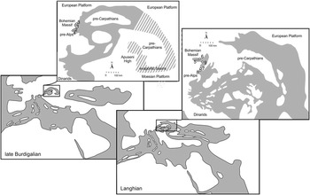
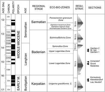
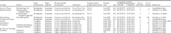
The present study focuses on lower and middle Miocene benthic assemblages of the Vienna Basin and the North Alpine Foreland Basin. These basins were part of the Central Paratethys, which ranged from southern Germany in the west to the Carpathian Foredeep in the Ukraine in the east, and from Bulgaria in the south to Poland in the north (Fig. 1). Due to the complex geodynamic history, a regional chronostratigraphic stage system (Fig. 2) is used in the Central Paratethys. We studied benthic mollusks from nine localities where the Karpatian (upper Burdigalian) and the lower Badenian (Langhian) strata were suitable for bulk sampling (Fig. 1, Table 1). All samples are from unlithified, siliciclastic pelitic, sandy, and gravelly sediments, are characterized by aragonite and calcite preservation, and were sieved through a 1 mm mesh. Detailed paleoecological and taphonomic studies have been published on some of the sections (see references in Table 1). The shell beds of the respective localities were deposited between 16.5 and 13.8 Ma and belong to five formations, three third-order stratigraphic sequences (Tb.2.2 to Tb.2.4 of Hardenbol et al. Reference Hardenbol, Thierry, Farley and Jacquin1998), and mostly capture highstand systems tracts (HST); only one section belongs to a transgressive systems tract (TST) (Strauss et al. Reference Strauss, Harzhauser, Hinsch and Wagreich2006). Samples from the TST show no evidence of extensive condensation or reworking (Zuschin et al. Reference Zuschin, Harzhauser and Mandic2007). Previous studies show that benthic assemblages of the two stages were similarly distributed along a single depth-related environmental gradient over less than 3 Myr (Zuschin et al. Reference Zuschin, Harzhauser and Mandic2011, Reference Zuschin, Harzhauser, Hengst, Mandic and Roetzel2014).
Karpatian and Badenian paleogeography of the Central Paratethys (modified after Rögl [Reference Rögl1998] and Kováč et al. [Reference Kováč, Andreyeva-Grigorovich, Brzobohatý, Fodor, Harzhauser, Oszczypko, Pavelic, Rögl, Saftic, Sliva and Stranik2004, Reference Kováč, Andreyeva-Grigorovich, Bajraktarevic, Brzobohaty, Filipescu, Fodor, Harzhauser, Nagymarosy, Oszczypko, Pavelic, Rögl, Saftic, Sliva and Studencka2007]) with approximate positions of studied localities in Austria. Karpatian (i.e., late Burdigalian) localities include: 1. Laa a.d. Thaya; 2. Kleinebersdorf; 3. Neudorf bei Staatz; 4. Korneuburg SPK. Lower Badenian (i.e., Langhian) localities include: 5. Grund; 6. Immendorf; 7. Gainfarn; 8. St. Veit; 9. Niederleis. White = land; gray = sea.

Stratigraphic details for the studied sections.

Provenance data of the studied assemblages. Third-order stratigraphic sequences (Tb.2.2 to Tb.2.4) after Hardenbol et al. (1998)

For the purpose of this study, we focus on the major transitions along the depth and salinity gradient: intertidal–subtidal and brackish–normal marine, respectively. Consequently, we environmentally assign samples to two water-depth and two salinity zones. Water-depth zones are (1) the intertidal to very shallow sublittoral (≤1 m water depth), and (2) the deeper sublittoral (a few meters to several tens of meters of water depth), hereafter termed “intertidal” and “subtidal,” respectively. Salinity zones are (1) brackish water (represented by estuarine succession in the Korneuburg Basin; Zuschin et al. Reference Zuschin, Harzhauser, Hengst, Mandic and Roetzel2014) and (2) normal marine (successions in the Vienna Basin and Alpine Foredeep; Zuschin et al. Reference Zuschin, Harzhauser and Mandic2011). The combination of these two environmental gradients generates four broad habitats: estuarine intertidal, marine intertidal, estuarine subtidal, and marine subtidal. We trace faunal turnover between the intertidal and subtidal zones in conditions of either predominantly brackish (estuarine depth gradient) or normal salinity (marine depth gradient). For the salinity gradient, we evaluate community change between the brackish and normal salinity regime in either the intertidal (intertidal salinity gradient) or subtidal zone (subtidal salinity gradient). The paleoenvironmental designations of samples rely on the paleogeographic positions of localities, actualistic environmental requirements of dominant molluscan taxa, and data from foraminifera and stable isotope analyses (for details, see Zuschin et al. [Reference Zuschin, Harzhauser and Mandic2011, Reference Zuschin, Harzhauser, Hengst, Mandic and Roetzel2014] and case studies cited in Table 1).
Data Analyses
Small sample sizes may obscure paleoecological patterns (e.g., Forcino Reference Forcino2012). We therefore removed all samples with fewer than 50 individuals from the data set. As in many other paleoecological studies, the number of samples varied between habitats, depending on the number and outcrop conditions of fossiliferous localities (Table 2). First, to account for the unequal number of samples per habitat, 15 samples were drawn without replacement from each environmental zone, which is the minimum number of samples per habitat. Second, the size of each selected sample was standardized to 50 individuals by rarefaction to account for the unequal number of specimens. This subsampling procedure was repeated 1000 times to obtain mean values and corresponding 95% confidence intervals (CIs) for all measured statistics. All subsequent analyses were performed on such double-standardized data sets (Tomašových and Kidwell Reference Tomašových and Kidwell2009a).
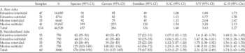
Number of samples, specimens (N) and taxa, and taxonomic ratios for each habitat in the original data set and corresponding median values for the double-standardized data (1000 random sets of 15 samples per habitat and 50 individuals per sample drawn without replacement from the ordinal data). S/G, ratio of species richness to genus richness; S/F, ratio of species richness to family richness; G/F, ratio of genus richness to family richness.

Species abundance data were (1) aggregated into genera and families and (2) subjected to a sequence of transformations that gradually shift the emphasis of analyses from the most dominant to rare taxa (untransformed, square-root-transformed, and fourth-root-transformed proportions, and presence–absence data). The paleocommunities of the four habitats were characterized by rank abundance distributions, Hulbert’s probability of an interspecific encounter (PIE) diversity index (a measure of evenness), and the proportion of singletons (a measure of rarity) for all three taxonomic levels. Because the ratio of lower to higher taxa can strongly influence the results of taxonomic sufficiency analyses (e.g., Wright et al. Reference Wright, Chessman, Fairweather and Benson1995), we calculated ratios of species to genus and species to family for the total assemblage and all four habitats.
Nonmetric multidimensional scaling (NMDS) based on the Bray-Curtis dissimilarity was used to visualize the effects of taxonomic and numerical resolution on variation in community composition among samples from different environmental zones (Clarke Reference Clarke1993). To facilitate the comparison of the results, NMDS solutions were rotated using principal components analysis, so that the variance among samples was maximized along the first axis, and rescaled according to the underlying dissimilarity matrix using the metaMDS function (Oksanen et al. Reference Oksanen, Blanchet, Kindt, Legendre, Minchin, O’Hara, Simpson, Solymos, Stevens and Wagner2015). Because each double-standardized subsample of the full data set requires a separate ordination, we show NMDS for a single, randomly chosen subsample and compare it with the ordination of the complete nonstandardized data set to evaluate the consistency of the results.
Similarity in multivariate community patterns between the three taxonomic levels was evaluated by computing Spearman rank correlations (ρ) between pairs of Bray-Curtis dissimilarity matrices. This method is commonly applied in assessments of taxonomic sufficiency in marine pollution studies (Somerfield and Clarke Reference Somerfield and Clarke1995; Bevilacqua et al. Reference Bevilacqua, Terlizzi, Claudet, Fraschetti and Boero2012). The underlying assumption is that species and proportional abundances are the best choices to detect changes along ecological gradients. The permutation-based Mantel test was used to determine the significance of the correlation. We used the same procedure to assess the congruence between different numerical resolutions of the data. In this case, the proportional abundance data set served as a baseline against which other transformations were compared.
The sensitivity of habitat discrimination to changes in taxonomic and numerical resolution was evaluated by tracking the proportion of multivariate variation in the assemblage composition explained by the environmental classification at different levels of taxonomic aggregation and numerical transformation. For this purpose, we used permutational multivariate analysis of variance (PERMANOVA; Anderson Reference Anderson2001) based on Bray-Curtis dissimilarities and samples grouped into four habitats. PERMANOVA partitions sums of squared dissimilarities within and among habitats and constructs a pseudo–F-statistic from a dissimilarity matrix analogous to the F-ratio in ANOVA. Random permutations of observations among habitats are then used to obtain p-values for the null hypothesis of no difference in the location of centroids of habitats. We performed PERMANOVA and a Mantel test on double-standardized data so that multivariate dispersion of individual habitats is not obscured by differences in the number of samples (Anderson and Walsh Reference Anderson and Walsh2013); the distribution of p-values across all subsampling iterations was used for statistical inference. The proportion of variation in the whole data set estimated by PERMANOVA (R 2) served as a measure of compositional separation between the four habitats and corresponds to the variation explained simultaneously by depth and salinity. Separate analyses were performed on subsets of the data representing pairs of habitats along a gradient (e.g., marine intertidal and marine subtidal samples) to check whether decreasing taxonomic and numerical resolution have consistent effects on both environmental gradients. All statistical analyses were performed in R, Version 3.2 (R Core Team 2015) using the ‘vegan’ package (Oksanen et al. Reference Oksanen, Blanchet, Kindt, Legendre, Minchin, O’Hara, Simpson, Solymos, Stevens and Wagner2015).
Results
Paleocommunities of the Four Habitats
Much higher numbers of species, genera, and families are recorded from marine subtidal samples compared with the other three habitats, which show similarly low richness (Table 2). At all taxonomic levels, the marine subtidal assemblage is also characterized by a very distinct rank abundance distribution (Supplementary Fig. S1) and by the highest share of rare taxa (Supplementary Fig. S2). Evenness as measured by PIE is higher in the two subtidal habitats (Supplementary Fig. S2). The ratios of taxonomic levels tend to be slightly higher in marine than estuarine habitats, but they are all consistently low (Table 2). The species:family ratio in the size-standardized data set never exceeds 2.0 for individual habitats and reaches 2.31 for the total assemblage; species:genus and genus:family ratios are correspondingly lower (Table 2).
Rank Correlation between Bray-Curtis Similarity Matrices
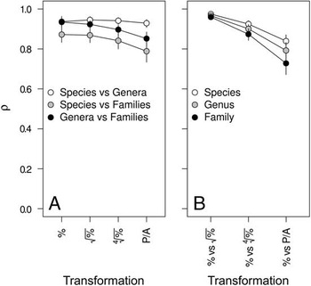
In the total data set, Spearman rank correlations between dissimilarity matrices representing different taxonomic levels are high and significant for all numerical transformations (ρ=0.79–0.95; for all comparisons, Mantel test median p=0.001; Fig. 3A). For proportional abundances, the correlation is similarly strong for species versus genera and genera versus families and is somewhat lower for species versus families. The effects of numerical transformation are visible only for the latter two comparisons as a decrease in rank correlation for fourth-root-transformed percentages and presence–absence data (Fig. 3A). Rank correlations between dissimilarities at different numerical levels are also high (ρ=0.73–0.98, p=0.001; Fig. 3B). The square-root-transformed proportional abundances show the strongest correlation with proportional abundances, and correlations decrease with increasing level of numerical transformation. This decrease is smallest for species and strongest for families (Fig. 3B).
Spearman rank correlation between Bray-Curtis dissimilarity matrices in the total data set. A, Correlation between taxonomic levels at different numerical resolutions. Numerical transformation of proportional abundances increases from left to right along the x-axis. %, no transformation;
 $\sqrt \%\, $
, square-root transformation;
 $\root 4 \of \%\, $
, fourth-root transformation; P/A, presence–absence transformation. B, Correlation between proportional abundance data and higher levels of numerical transformation. Shown are mean values and 95% CI for double-standardized data; see “Materials and Methods” for details.

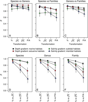
When subsets of the data representing pairs of habitats positioned along the gradients are considered separately, rank correlations between matrices representing different taxonomic levels are similar to those in the total data set (ρ>0.8; Fig. 4A–C). Two exceptions are correlations for the salinity gradient in intertidal habitats (marine and estuarine intertidal samples), which strongly decrease with numerical transformation (from 0.96 to 0.60 for comparison of species- and family-level matrices), and the rank correlation of species versus families in subtidal habitats, which is stable at a relatively low ρ around 0.75 (Fig. 4B). In all four environments, rank correlations are highest for proportional abundances (vs. square-root-transformed proportional abundances) and decrease with increasing numerical transformation. Although this drop is especially strong in estuarine and intertidal habitats (down to ρ=0.37 for intertidal samples; Fig. 4D–F), all correlations remain significant (Mantel test median p=0.001 in all cases; Supplementary Fig. S3).
Spearman rank correlation (mean values and 95% CI for double-standardized data) between Bray-Curtis dissimilarity matrices along environmental gradients between taxonomic levels at different numerical resolutions (A–C) and for proportional abundance data and higher levels of numerical transformation (D–F). For an explanation of the x-axis, see Fig. 3.

Ordination Patterns
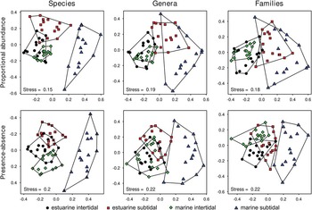
NMDS ordinations differ substantially between taxonomic and numerical levels of analysis (Fig. 5), even though the underlying dissimilarity matrices are significantly and positively correlated. The relative positions of samples representing the four habitats change with decreasing numerical and taxonomic resolution, although with varying directions and intensities (Fig. 5, Supplementary Fig. S4). Ordinations based on the nonstandardized data set show very similar patterns (Supplementary Fig. S5). The segregation between the marine and estuarine intertidal is weakly affected by the loss in taxonomic resolution but is much stronger for presence–absence data than for proportional abundances. The differences between marine intertidal and marine subtidal are high and remain equally strong at all levels of numerical and taxonomic transformation. For abundance data, the estuarine subtidal shifts from overlaps with the estuarine intertidal (species) to strong overlap with the marine subtidal (genus and family). For presence–absence data, the differences between the marine subtidal and all other habitats, and the differences between the estuarine subtidal and the two intertidal habitats, decrease from species to family level (Fig. 5).
Effect of taxonomic aggregation and numerical transformation on NMDS ordination patterns in a double-standardized subsample of the total data set. Results for square-root-transformed and fourth-root-transformed proportions were omitted for clarity and showed patterns intermediate between proportional and presence–absence data.

Proportion of Variation in the Data Set Explained by Environmental Classification
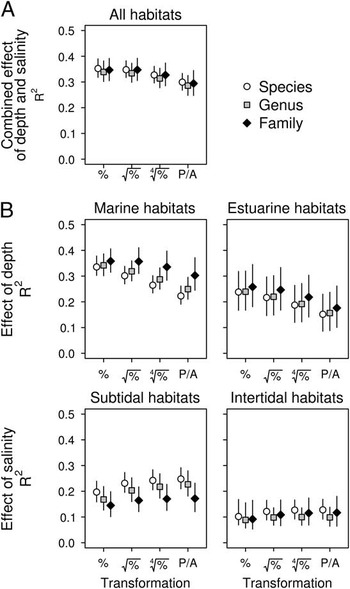
At all taxonomic and numerical levels, PERMANOVA detects significant differences in molluscan assemblages among the four habitats (p=0.001). Water depth and salinity explain together between 29% and 35% of the compositional variability (Fig. 6A). R 2 is highest for untransformed and square-root-transformed proportions and decreases slightly with further numerical transformation. The differences between taxonomic levels are minor at all levels of numerical resolution (Fig. 6A).
Effect of taxonomic aggregation and numerical transformation on the proportion of compositional variation explained by environmental classification as estimated by PERMANOVA (mean values and 95% CI for double-standardized data) in the total data set (A, all four habitats considered) and along environmental gradients (B, pairwise comparisons between habitats). For an explanation of the x-axis, see Fig. 3.

This relatively high percentage of variation explained in the total data set (Fig. 6A) masks significant variation in the strength of the environmental effects along the two gradients, because completely different patterns are evident for the separation of depth and salinity zones (Fig. 6B). On one hand, proportional abundances separate best between depth zones (intertidal vs. subtidal), and any further numerical transformation decreases their ability to distinguish between habitats. Family data always perform better than genus and species data. On the other hand, in contrast to water depth, the ability to separate between salinity zones (estuarine vs. marine) increases gradually with numerical transformation toward presence–absence data and is always better for species than for genera and families (Fig. 6B). The intertidal and subtidal habitats are better separated in the marine (R 2=0.22–0.36) than in the estuarine environment (R 2=0.15–0.26). In contrast, communities from habitats of different salinity levels are more distinct in the subtidal (R 2=0.14–0.25) than in the intertidal zone (R 2=0.09–0.13; Fig. 6B). The number of significant pairwise PERMANOVA tests between habitats is little affected by the taxonomic and numerical resolution (median p=0.001 in all cases; Supplementary Fig. S6). The exception is the comparison of the two intertidal habitats, where median p-values, all below 0.05, decrease with increasing severity of transformation and are consistently lower for species than for genera and families (Supplementary Fig. S6).
Discussion
Taxonomic and Numerical Sufficiency with Respect to Explicit Environmental Gradients
This study suggests that there is no unique appropriate taxonomic and numerical resolution to reveal the changes that occur along different environmental gradients. Moreover, even though the differences between molluscan assemblages from the four habitats remain significant irrespective of taxonomic aggregation and numerical transformation, the patterns in ordination and the proportion of variation explained by the environmental classification change in a complex manner (Figs. 5 and 6). The effect of change with depth, as estimated by R 2, is strongest for family data, decreases gradually with numerical transformation, and is higher in marine than in estuarine habitats. In contrast, the effect of shift in salinity is highest for species-level data, increases gradually with numerical transformation, and is higher in subtidal than in intertidal habitats (Fig. 6B). Because of these opposing patterns, the global R 2—measuring the combined effect of both gradients in the total data set—is little affected by a shift in taxonomic or numerical resolution (Fig. 6A). However, when each environmental factor is considered separately, the changes in the apparent strength of their effects lead to contrasting conclusions about the relative importance of depth and salinity in structuring benthic communities.
Most studies on numerical and taxonomic resolution have dealt with sufficiency and cost-efficiency (e.g., Ellis Reference Ellis1985; Warwick Reference Warwick1988; Dauvin et al. Reference Dauvin, Gomez Gesteira and Salvande Fraga2003; Bevilacqua et al. Reference Bevilacqua, Terlizzi, Claudet, Fraschetti and Boero2012), but the effects of transformation on the effects of environmental gradients on community composition are rarely considered (Chapman Reference Chapman1998; Anderson et al. Reference Anderson, Connell, Gillanders, Diebel, Bloms, Daunders and Landers2005; Dethier and Schoch Reference Dethier and Schoch2006; Tomašových and Kidwell Reference Tomašových and Kidwell2009b). On one hand, studies that have used multivariate analyses to evaluate numerical and taxonomic sufficiency have reported similar results: statistically significant differences between environmentally defined groups of samples are retained at higher levels of numerical transformation and taxonomic aggregation at least up to the family level. On the other hand, however, the degree of separation between assemblages from different environments (measured by R 2 or by other metrics, such as R in analysis of similarities; Clarke Reference Clarke1993) can change considerably and can vary among studies and among regions (Somerfield and Clarke Reference Somerfield and Clarke1995; Olsgard et al. Reference Olsgard, Somerfield and Carr1998; Pandolfi Reference Pandolfi2001; Bertasi et al. Reference Bertasi, Colangelo, Colosio, Gregorio, Abbiati and Ceccherelli2009). Finally, the overall ordination pattern can also be affected (Pandolfi Reference Pandolfi2001; Forcino et al. Reference Forcino, Stafford and Leighton2012).
The results of this study underline the observations that statistical significance of environmental forcing of community differentiation is rarely affected by numerical transformations or taxonomic aggregation up to the family level. Nonetheless, inferences on the relationships between the assemblages based on unconstrained ordination patterns and, more importantly, quantitative evaluations of the environmental effect size (i.e., the magnitude of compositional separation among different habitats) depend strongly on the taxonomic and numerical scale of the analyses, affecting paleoecological interpretations on the assembly of communities along environmental gradients.
Rank correlation between Bray-Curtis similarity matrices at different taxonomic levels is frequently used in analyses of taxonomic sufficiency (e.g., Somerfield and Clarke Reference Somerfield and Clarke1995; De Biasi et al. Reference De Biasi, Bianchi and Morri2003; Włodarska-Kowalczuk and Kędra Reference Włodarska-Kowalczuk and Kędra2007). The underlying assumption is that species and proportional abundances are the best choice to detect changes along ecological gradients. Decrease in the rank correlation coefficient at higher taxonomic levels and increasing numerical transformation (vs. analysis at the species level and proportional data) is interpreted as an information loss (Karakassis and Hatziyanni Reference Karakassis and Hatziyanni2000).
Results are in line with these previous studies, in that rank correlations of data sets between species and higher taxa (most notably genera and families) are very high for proportional abundance data (e.g., Somerfield and Clarke Reference Somerfield and Clarke1995; De Biasi et al. Reference De Biasi, Bianchi and Morri2003; Włodarska-Kowalczuk and Kędra Reference Włodarska-Kowalczuk and Kędra2007; Souza and Barros Reference Souza and Barros2015). Low taxonomic resolution combined with numerical data transformation may lead to putative information loss, that is, community patterns different from those observed on the species level (Olsgard et al. Reference Olsgard, Somerfield and Carr1998; Lasiak Reference Lasiak2003; Musco et al. Reference Musco, Mikac, Tataranni, Giangrande and Terlizzi2011). Also, in our case the rank correlations between data sets decrease disproportionally with higher orders of numerical transformation, most notably in the intertidal habitats. The reduction to presence–absence data, however, can still yield a good discrimination of habitats, as indicated by statistically significant differences between habitats at all levels of numerical transformation. The segregation between assemblages can even improve relative to the abundance data, as observed along the salinity gradient in this data set. This does not mean that qualitative sampling alone is sufficient to discriminate communities from different environments: presence–absence data derive from an intensive quantitative sampling program, not from a priori qualitative sampling. Occurrence data are therefore suitable as long as they derive from intensive random sampling using bulk samples, which are used to record the presence of species.
Effects of Numerical Resolution on Detecting Environmental Gradients
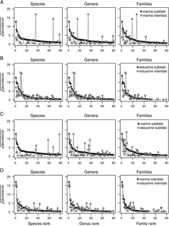
In contrast to previous studies, our work shows that taxonomic aggregation and the loss in numerical resolution may actually improve the ability to capture environmental gradients. Therefore, low concordance with species-abundance data does not necessarily translate to loss of environmental resolution. Moreover, the two gradients respond in contrasting ways to changes in numerical and taxonomic scale. This variation in the outcome of multivariate analyses reflects different magnitudes of turnover in taxonomic composition and shifts in abundance of taxa between habitats. This is evident when comparing habitat-specific species pools after pooling their constituent samples (Fig. 7). Much higher evenness and richness characterizes the marine subtidal (vs. the three other habitats; Supplementary Figs. S1 and S2). Consequently, the marine subtidal shares few taxa along the depth gradient with the marine intertidal, and those that are shared have very different abundances, irrespective of the taxonomic level considered (Fig. 7A). In contrast, the shift in abundance among the few species shared along the salinity gradient between the marine and estuarine subtidal is not as strong, and the differences decrease among genera and families (Fig. 7C). The overlap in species composition of habitats along the estuarine depth gradient and along the intertidal salinity gradient is much larger (Figs. 7B,D). Along the depth gradient, abundances between estuarine species differ strongly, but the change is very small for species shared between the two intertidal habitats. In other words, proportional abundance data maximize the separation of habitats along the bathymetric gradient because, in addition to a change in taxonomic composition (species identity), there is a strong shift in the relative abundance of species that do cross the intertidal–subtidal transition (Fig. 7). Presence–absence data, in turn, perform better for the salinity gradient, because changes in abundance are less pronounced here and at least some taxa tend to dominate both estuarine and marine assemblages.
Changes in the abundance of dominant taxa between habitats along the depth gradient (A and B) and along the salinity gradient (C and D). Each point represents the absolute abundance of a taxon in a given habitat after pooling all constituent samples in double-standardized data (mean value across 1000 resampling iterations; the total abundance in each habitat always sums up to 750 individuals). Note much stronger shift in abundance across the intertidal–subtidal transition (i.e., along the depth gradient).

Effects of Taxonomic Resolution on Detecting Environmental Gradients
Aggregating species into higher taxa can result in good community and paleocommunity discrimination for several reasons. First, closely related species often have similar environmental requirements (e.g., Wright et al. Reference Wright, Chessman, Fairweather and Benson1995), that is, they are characterized by high niche conservatism (Wiens and Graham Reference Wiens and Graham2005). This is likely true for many molluscan species (e.g., Stanley Reference Stanley1970; Saupe et al. Reference Saupe, Hendricks, Portell, Dowsett, Haywood, Hunter and Lieberman2014), and grouping them into higher taxa would therefore preserve the environmental signal. For example, marine congeneric bivalves tend to show conservative latitudinal range limits, likely reflecting similar thermal preferences (Roy et al. Reference Roy, Hunt, Jablonski, Krug and Valentine2009). Second, if the number of species in higher taxa is low, then the patterns of higher taxa should closely follow those of the constituent species (e.g., Pandolfi Reference Pandolfi2001; Bavilacqua et al. 2012). In this data set, the average ratio of taxonomic levels is generally very low and differences in taxonomic ratios between habitats are small. Third, for abundance data, the pattern of the most abundant species will drive the analysis at a higher taxonomic level (James et al. 1995). Strong dominance of one particular species in a higher taxon is also a typical feature of these samples. Fourth, reducing taxonomic resolution also reduces the number of variables and the number of zeros in the data set (Vanderklift et al. Reference Vanderklift, Ward and Jacoby1996); this may dampen the natural variability in patterns in community composition (Ferraro and Cole Reference Ferraro and Cole1990; Frost et al. Reference Frost, Carpenter and Kratz1992). This latter factor, combined with high niche conservatism, can be responsible for the improved separation of habitats along the depth gradient when family-level data are used. Taxonomic aggregation will average out patchy occurrences of species across individual samples if families tend to group species with similar bathymetric preferences. In contrast, lumping species to genera and families reduces the segregation between estuarine and marine assemblages, suggesting that tolerance for reduced salinity varies strongly among closely related species.
Multiscale Analyses rather than Selecting a Best Single Scale
This study supports the view that different processes drive variation in a given ecosystem at different levels of taxonomic and numerical resolution, and thus community patterns should be analyzed and interpreted at more than one scale (e.g., Rahel Reference Rahel1990; Anderson et al. Reference Anderson, Connell, Gillanders, Diebel, Bloms, Daunders and Landers2005). These findings have implications for studies evaluating temporal and spatial community persistence (DiMichele et al. Reference DiMichele, Behrensmeyer, Olszewski, Labandeira, Pandolfi, Wing and Bobe2004). The choice of numerical resolution, the exclusion of rare taxa, and the analytical approach all apparently affect the tests for stability (Visaggi and Ivany Reference Visaggi and Ivany2010). Benthic faunas show stability at larger scales (Ivany et al. Reference Ivany, Brett, Wall, Wall and Handley2009) and when presence–absence data are used (Brett and Baird Reference Brett and Baird1995), but not at small scales (Bonuso et al. Reference Bonuso, Newton, Brower and Ivany2002) and when abundance data are used (Brett et al. Reference Brett, Bartholomew and Baird2007). However, the patterns of community turnover along environmental gradients can also show various degrees of stability and change through time (Holland and Patzkowsky Reference Holland and Patzkowsky2007; Bonelli and Patzkowsky Reference Bonelli and Patzkowsky2008; Balseiro et al. Reference Balseiro, Waisfeld and Vaccari2011; Kowalewski et al. Reference Kowalewski, Wittmer, Dexter, Amorosi and Scarponi2015; Balseiro Reference Balseiro2016). For example, higher temporal persistence of molluscan communities in offshore than in onshore habitats is visible only at genus and family levels at timescales exceeding several millions of years (Tomašových et al. Reference Tomašových, Dominici, Zuschin and Merle2014). Expression of community gradients at different numerical scales depends on the relative importance of changes in species identity as opposed to changes in relative abundance among habitats, which in turn reflects the degree of ecological specialization. Effects of taxonomic aggregation, in contrast, are primarily governed by the strength of niche conservatism and by the ratio of species to higher taxa related to diversification rates (e.g., Foote Reference Foote2012). Therefore, explicit comparison of paleocommunity patterns recovered at multiple numerical and taxonomic scales along environmental gradients can provide information on ecological and evolutionary dynamics underlying ecological gradients and their relative stability.
Conclusions
Analysis of the Miocene metacommunity of the Central Paratethys shows that taxonomic aggregation and numerical transformation of data result in very different ordination plots. Rank correlations of Bray-Curtis similarity matrices between species and the higher levels (genus, family) are very high for proportional abundance data in the whole data set and in individual habitats, but they decrease disproportionally strongly with higher orders of numerical transformation, most notably in the two intertidal habitats. This effect, however, is not much stronger for families than for species, and we therefore conclude that numerical transformation is responsible for most of the differences observed in these comparisons.
The proportion of variation explained by environmental classification shows contrasting patterns along the water-depth and salinity gradients: compositional segregation between assemblages representing different habitats is maximized with family-level abundance data along the depth gradient and with species-level presence–absence data along the salinity gradient. Changes of patterns in ordination and in the proportion of variation in community composition related to environmental factors are complex, because turnover of taxa and their abundances along gradients is not uniform.
These results suggest that there is no single best taxonomic and numerical level of resolution for the analysis of ecological data sets: the ability to discriminate an environmentally driven community gradient is a function of a gradient itself and thus can be strongly context specific. Importantly, the “best” resolution—the one maximizing the separation between assemblages along a gradient—depends on the nature of response of communities to the environmental factor considered. Consequently, changes in multivariate community patterns emerging when data are analyzed at different taxonomic or numerical levels should not be regarded as an artifact or a loss of ecological information. Rather, the different results yield complementary insights into processes shaping ecological gradients.
Acknowledgments
This study was financially supported by projects P13745-Bio and P19013-B17 of the Austrian Science Fund (FWF). R.N. was supported by a uni:doc fellowship of the University of Vienna, and A.T. by the Slovak Scientific Grant Agency (VEGA 0136-15). Tom Olszewski, an anonymous colleague, and Michael Stachowitsch provided helpful comments on the manuscript.
Supplementary materials
Data available from the Dryad Digital Repository: http://dx.doi.org/10.5061/dryad.r7s92