Moderator (Miss C. R. Drummond, F.I.A.): The 2024 winners of the prestigious Brian Hey Prize now present the findings from their award-winning research on parameterising capital modelling volatility in the context of changing business volumes.

The paper addresses a critical challenge that is faced by both capital modelling experts and validators of capital models. When you have assessed your volatility assumptions based on a specific book of business, how do you appropriately reflect changes to your portfolio size and structure for a future capital model?

The approach the team has come up with bridges a key gap in current practice. It offers a helpful rule of thumb, which strikes a balance between technical robustness and real-world applicability. This work goes beyond an academic contribution; it is highly relevant and actionable for anyone working in the capital modelling and validation space.

Our speakers for this evening are Neil Gedalla, Adam Smylie and Jade Lagrue.

Neil is a Principal at Lane Clark & Peacock (LCP) with extensive experience in capital modelling and validation work. Neil has held a variety of roles across the insurance industry, and he is also a member of the IFoA’s General Insurance Capital Research Group.

Adam is an Associate Consultant at LCP with experience across capital, validation, reserving, and risk management. Prior to joining LCP, Adam worked at Probitas 1492 as a capital modelling analyst.

Jade is an Associate Consultant at LCP, specialising in internal model validation, reserving, and reinsurance modelling. Jade supports LCP’s analytics modelling, which is helping to develop software to assess reserve risk and analyse trends in reserve deteriorations. She is the co-chair of the London Market Student Group.

Mr N. M. Gedalla, F.I.A.: The problem, or rather the series of related problems, that we are trying to solve concern what to do when volatility assumptions become disconnected from the volumes that they were originally derived from, in the context of capital modelling. The relationship between volume and volatility in the context of insurance is fundamental. The principle by which insurance works is that by bringing together lots of risks, we can create a more predictable outcome. This increased diversification between risks means that an insurance company has a more predictable outcome than any of the individual underlying risks. The question we are focused on is what is that relationship? Can we boil that relationship down to a simple formula that allows us to manipulate capital modelling assumptions?

We set this out in the context of the actuarial control cycle. I will specify the problem that needs to be solved. Adam (Smylie) and Jade (Lagrue) will then talk through the analysis that we have done to try to find a solution to these problems. They will focus on two different approaches. The first approach looks at actual historical reserve movements, and the relationship between volume and volatility that we see within that. The second approach looks at bootstrapping techniques to try to derive what we see as the theoretical volatility and the relationship that has with reserve volume. We will then talk through the results of the LCP survey benchmarking data, which we collate on an annual basis to help our clients understand what the market is doing in terms of selecting volatility parameters. Finally, I will talk a little bit about the overall results, some use cases, and what we see as potential next steps for research.

I will begin by specifying the problem, and provide some background about what we are trying to do here. We have identified some case studies that demonstrate how volatility assumptions can be disconnected from the volume assumptions that they were derived from. Starting with reserve risk, in capital modelling the parameterisation of this risk often happens at a different point from when the assumptions are going to be used. A typical example of this might be just after the year end, when capital modellers are thinking about what the coefficient of variation might be for the different reserve books they are trying to model. Those parameters won’t be used in the model until the next year-end date. They might be rolled forward six or twelve months and, because the reserve volumes will have changed by that point, they will become disconnected from the volume assumptions they were derived from.

Another example is validation. Often validation involves trying to sense check a selected volatility parameter against some sort of benchmark. That might be another firm, a collection of other firms, or an industry level benchmark. That presents a problem because, as we know, stacking lots of risks together makes them more predictable and less volatile. Therefore, trying to compare an individual firm’s volatility selection with the market becomes complex because they are not determined on a like-for-like basis. We expect the market to have a lower volatility. How do we adjust one of these assumptions to ensure that we have a like-for-like comparison that is meaningful in a validation context?

Thirdly, sensitivity and scenario testing. Capital modellers are often asked to run models with different business plan assumptions. For example, they might be asked what the capital requirement would be if certain business lines increased, or if they were to stop writing certain classes of business. Changing the volume assumptions necessitates some sort of adjustment to the volatility if the results are going to be meaningful. However, if the capital modelling team is asked for lots of these scenarios in a short period of time, they won’t have the bandwidth to re-parameterise all the volatility assumptions to allow for the changes. They will need a more systemic way of algorithmically adjusting the volatility to allow for these changes in volume.

Finally, we think about new classes of business. Often capital modellers are required to parameterise lots of different classes of business. They might choose to focus on a subset of those for which they have extensive data volumes or which are the most material. They might need a quick way of calculating assumptions for the remaining classes. What we are thinking about here is a way to take a reference class of business (a larger book with a known volatility) and scale that volatility to become appropriate for a smaller class of business. For example, a class where there is insufficient data. Those case studies are examples of some of the problems that we are trying to solve.

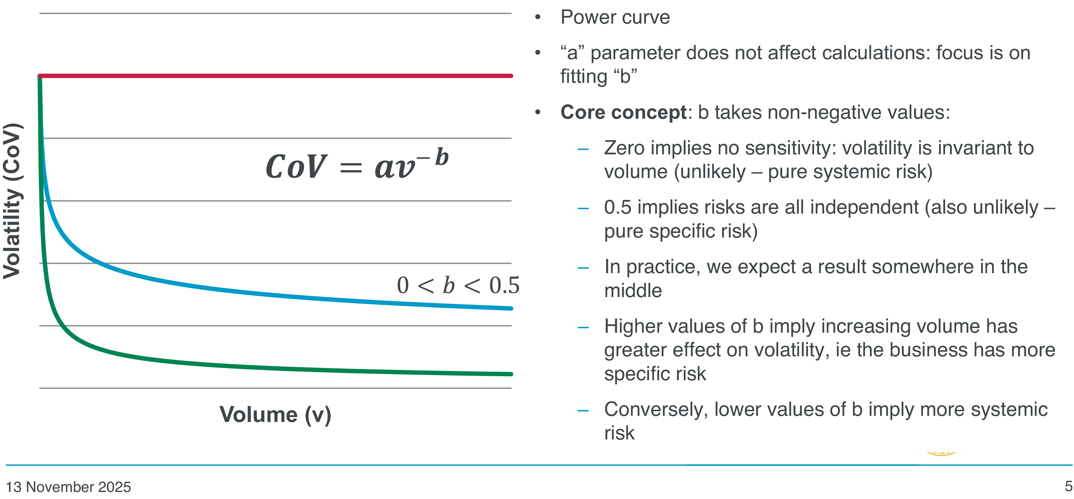
Figure 1 shows the model that, in our paper, is demonstrated to be a good fit to the historical data in terms of the relationship between volume and volatility. Specifically, we are saying that the coefficient of variation is equal to the volume, V, raised to the power -b (so an exponential parameter) multiplied by another constant, a. So there are two constants, a and b. We will show that the constant a can be dropped from the equation, as it cancels out and does not play any part in the formula. What we are doing is trying to find a value for the parameter b. There are lots of other models that we could use to fit this sort of relationship, where the volatility decreases as volume increases. In Appendix 4 of our paper we discuss another model, which we are calling the Theoretical Model. We demonstrate in our paper why the model in Figure 1 provides a better fit to the data than the other models.

Figure 1.

The model.

We have a few notes on the relationship and on parameter b. We can put some bounds on the relationship of how volatility decreases as volume increases. We know that b must take non-negative values. If b takes a negative value, that implies that the volatility increases as volume increases, which intuitively feels wrong. We know that diversification should result in a lower volatility, as volume increases. In practice, that is a lower bound of 0. The red horizontal line in Figure 1 is equivalent to a b parameter of 0. That implies no sensitivity of volatility to volume, and as volume increases, the volatility stays the same. That is equivalent to some sort of model or market where there is no diversification allowable. For example, this could be something like market risk, where buying more corporate bonds does not decrease your volatility because you are still exposed to the same underlying interest rate risk. In practice, in insurance, this very rarely happens as usually there will be some diversification and some specific risk. We do not have a market that is purely systematic risk, but that would be represented by that horizontal line. On the other side of the equation, we have an upper bound for the b parameter of 0.5. In the paper we go through the derivation that explains why that is the upper bound. Essentially, that is equivalent to a model in which all the risks are independent and there is no systemic volatility present at all. A model with purely specific risk results in an upper bound of 0.5. We are looking for a value for the b parameter in the range 0 to 0.5. In practice, we expect it to be somewhere in the middle. Where b falls in that range will be determined by the balance of specific and systemic risk within a given portfolio. Higher values of b, closer to 0.5, imply that we are looking at a case with more specific risk, and lower values of b imply that there is more systemic risk.

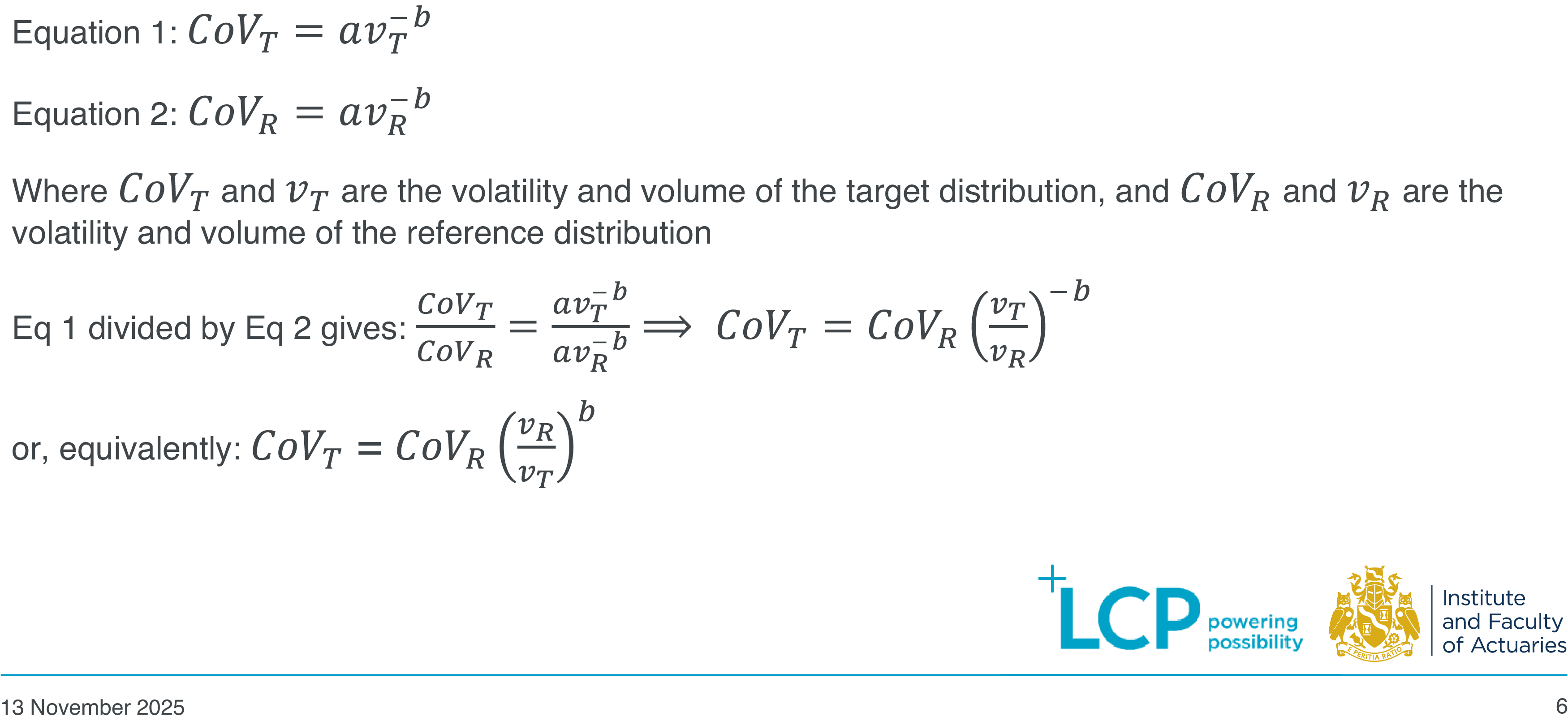
In Figure 2, we show the equation from Figure 1, with respect to a reference and a target distribution. The volatility of the target distribution is equal to a times v to the -b, and similarly for a reference distribution. Taking Equation 1 divided by Equation 2, we can show that the a parameters cancel. We can rearrange to show the coefficient of variation of the target distribution in terms of the volatility of the reference distribution, the volume of the target distribution, the volume of the reference distribution, and the parameter b. The volatility of the target distribution, which is what we are trying to solve for, is equal to the ratio of the volumes of the reference and target distribution, raised to the power of -b. That parameter acts as a scaling factor on the reference volatility, which is the parameter that we start with. Figure 2 shows two equivalent versions of this formula.

Figure 2.

Mathematics from Figure 1.

Moving on to the approach that we took, we are focusing on analysis on Schedule P data. Schedule P is a data set that results from the returns to the National Association of Insurance Commissioners (NAIC), which is the major regulator of insurers in the United States. We are focusing on that data set because it has lots of data in a standardised form that is very easy to download and query.

We are looking at two high-level approaches. We are thinking about these as complementary methods that each have different pros and cons, and different ways of looking at the data. The first approach is bucket analysis. Using bucket analysis, we take actual reserve movements that have been observed historically within the Schedule P data, and look at how volatile they are for different levels of the starting reserve volume. The second approach is bootstrapping of reserve triangles. This takes the triangles at a given point in time and applies a mechanical bootstrapping technique to come up with an estimated CoV. We look at how that estimated CoV changes as the volume of reserves increases.

We have done some additional analysis. We have considered class of business and/or cohort for both the bucket analysis and the bootstrapping. We are also looking at data from other geographical regions. The Australian Prudential Regulation Authority (APRA) provides some data, but it has weaknesses compared to Schedule P. In particular, there are significantly lower data volumes, and we do not have access to reserves. We only have incurred data from APRA and we can only apply bootstrapping, which is why it is not part of the main analysis.

As mentioned earlier, we have supplemented the main analyses with data from the annual LCP capital benchmarking survey, to see what data selected by practitioners can tell us. Does it imply that practitioners are taking proper account of the relationship between volume and volatility when they select CoVs?

The primary basis we are focusing on is around reserve risk, mainly because that is easier to calculate from the data sources that we have. We believe this would be applicable also to underwriting risk, but it is harder to demonstrate that. We are talking about a fundamental relationship between volume and volatility within the context of insurance. We do not see any reason why this would not also hold for underwriting risk, but tactically we have focused on reserve risk.

In terms of one-year and ultimate, the bucket analysis is based on one-year reserve movements, because that is easier to arrive at from the data. The bootstrapping is based on an ultimate bootstrap. A potential further research point would be to investigate whether there is a difference between one-year and ultimate. We do not believe that there would be, but it is not something that we have covered in our primary research.

Going back to the Schedule P data set, this is a large data set, with total reserves of just under $1 trillion. We were looking at 13 standardised reserving classes over a period of 12 completed calendar years. We have tried to preserve as much of the data as possible, in order to not bias the investigations, but we have done some data cleaning. We completed some light-touch cleaning to make sure that the data is as consistent with a typical capital modelling use case as possible. We have removed the obvious negative reserves and we have also removed some outlier reserve deteriorations. The cut-off point for that is 500%. Reserve deteriorations of more than 500% were excluded because, typically, capital modelling practitioners would not be dealing with movements of that size.

Figure 3 shows three things. On the left-hand axis, the chart shows the volume of reserves by class of business. On the right-hand axis, the dots show the number of reserving triangles. We split the data by duration of the tail. We split it into short, medium, and long-tailed business, because we had an intuition that there might be some differences in the b parameter between these groups.

Figure 3.

Schedule P dataset.

Mr A. Smylie, A.I.A.: I am going to talk through the methodology of the bucket analysis, the results, and some uncertainties that we have dealt with. Using the Schedule P data set we looked for a pattern that would explain the relationship between volume and volatility. The first step in the analysis was calculating the calendar year percentage reserve movements. Then, we wanted to relate each of those reserve movements to a corresponding reserve size. As an example, if we had a reserve of 100 million at the start of the year, and it went to 120 million at the end of the year, the reserve movement would be 20%. The corresponding reserve size would be 100 million, the reserve at the start of the year. In Schedule P we had 60,000 reserve movements, and Figure 4 shows each reserve movement plotted against the corresponding reserve size.

Figure 4.

Bucket analysis.

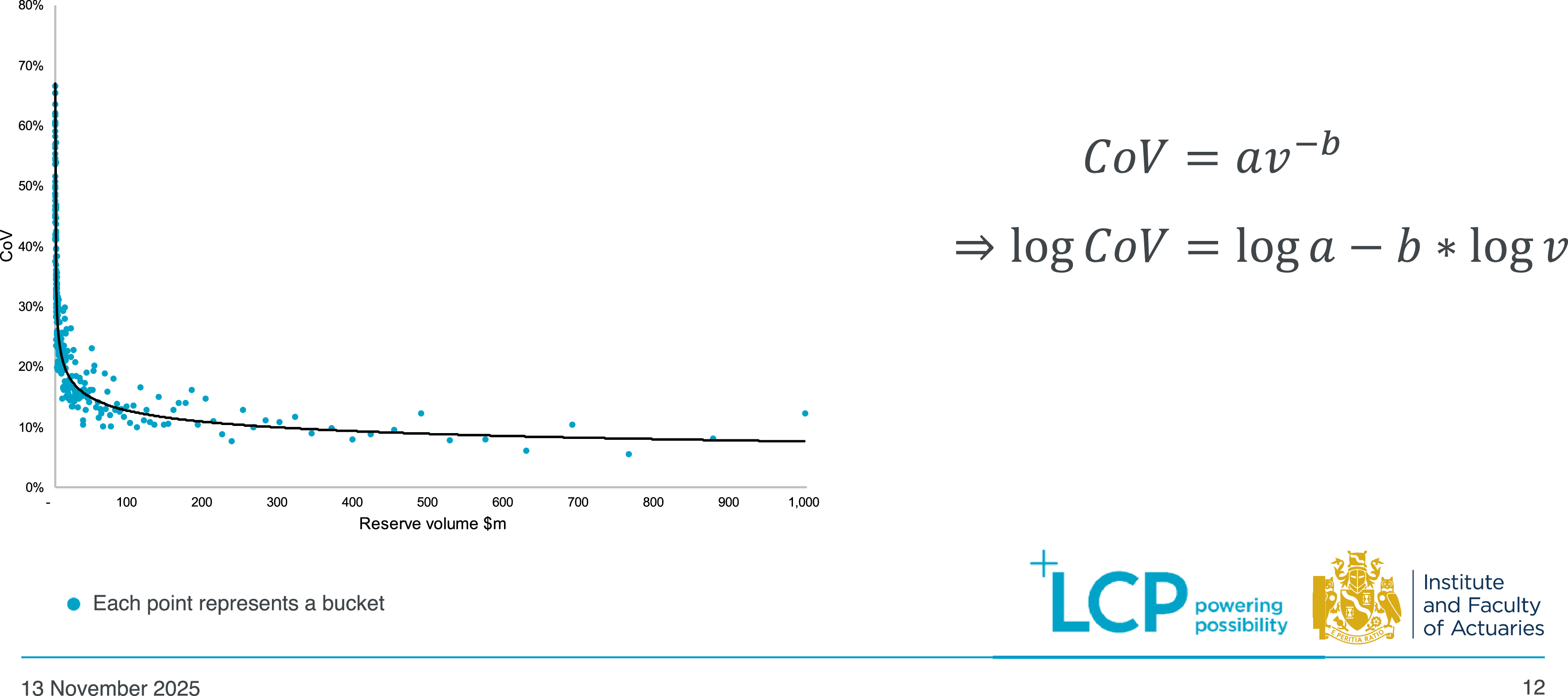
The first thing you can see from Figure 4 is the funnel shape of the reserve movements. It shows a tighter spread of reserve movements for larger reserve volumes. We were expecting some diversification and this confirms that diversification exists, at least in the US. At a high level, volatility decreases as volume increases. The next step is determining the rate of diversification as volume increases. We put the data into buckets based on reserve size. To do this, we order the reserve movements by reserve size and put the first 200 movements into the first bucket, the next 200 movements into the second bucket, and so on. In total we had 300 buckets. For each bucket we calculated a volume measure by taking the average reserve size of the data points in that bucket. We calculated the volatility measure for each bucket by taking the standard deviation of the percentage reserve movements. Figure 5 shows the volume measure plotted against the volatility measure, for each bucket.

Figure 5.

Bucket analysis – results part one.

We took logs of both sides of the equation, CoV=av ^-b and plotted the results. Figure 6 shows that this results in a graph with a negative gradient straight line. It shows a strong log linear relationship between reserve volume and volatility, and that implies the relationship CoV=av ^-b holds. Measuring the gradient of the line gives a value for b of 0.22.

Figure 6.

Bucket analysis – results part two.

You can see from Figure 6 that the blue dots are quite tightly packed around the trend line, so visually we can see that the model fit is good. We also calculated the R-squared metric, which is a measure of how much the model explains the variation of the data. The R-squared value is between 0 and 1, with 0 representing a very bad model fit and 1 representing a very good model fit. We calculated an R-squared value of 0.91, so it is a very good model fit.

We also attempted to fit a model CoV=av ^-b + $\gamma$ . Gamma here represents undiversifiable volatility. The question we were looking to answer was, as volume increases to something very large, does the volatility go to 0 or does it go to some minimum above 0? Is there a portion of reserve volatility that is undiversifiable or is it the case that as you increase reserve volumes to larger and larger volumes the volatility goes to 0? We found that gamma equal to 0 provided the best model fit, which is maybe a little bit unintuitive. As Neil (Gedalla) mentioned earlier, the b value represents the level of systemic and specific risk in the portfolio. A b value of 0.22 implies that there is some degree of systemic risk. However, the bucket analysis of Schedule P suggests that there is no evidence of undiversifiable volatility. This shows that you can have systemic risk but no undiversifiable volatility. If gamma was greater than 0, we would start to see the blue dots in Figure 6 level off horizontally for large enough reserve volumes. But Figure 6 shows that, even for very large reserve volumes, the blue dots continue in a downward fashion. The rightmost blue dots represent reserve volumes in the region of $50 billion, and up to those reserve volumes there is no evidence of undiversifiable volatility. If the data set was bigger, and we had reserve volumes in the hundreds of billions or the trillions, maybe we would start seeing this undiversifiable volatility, but there is no evidence of it in the Schedule P data set.

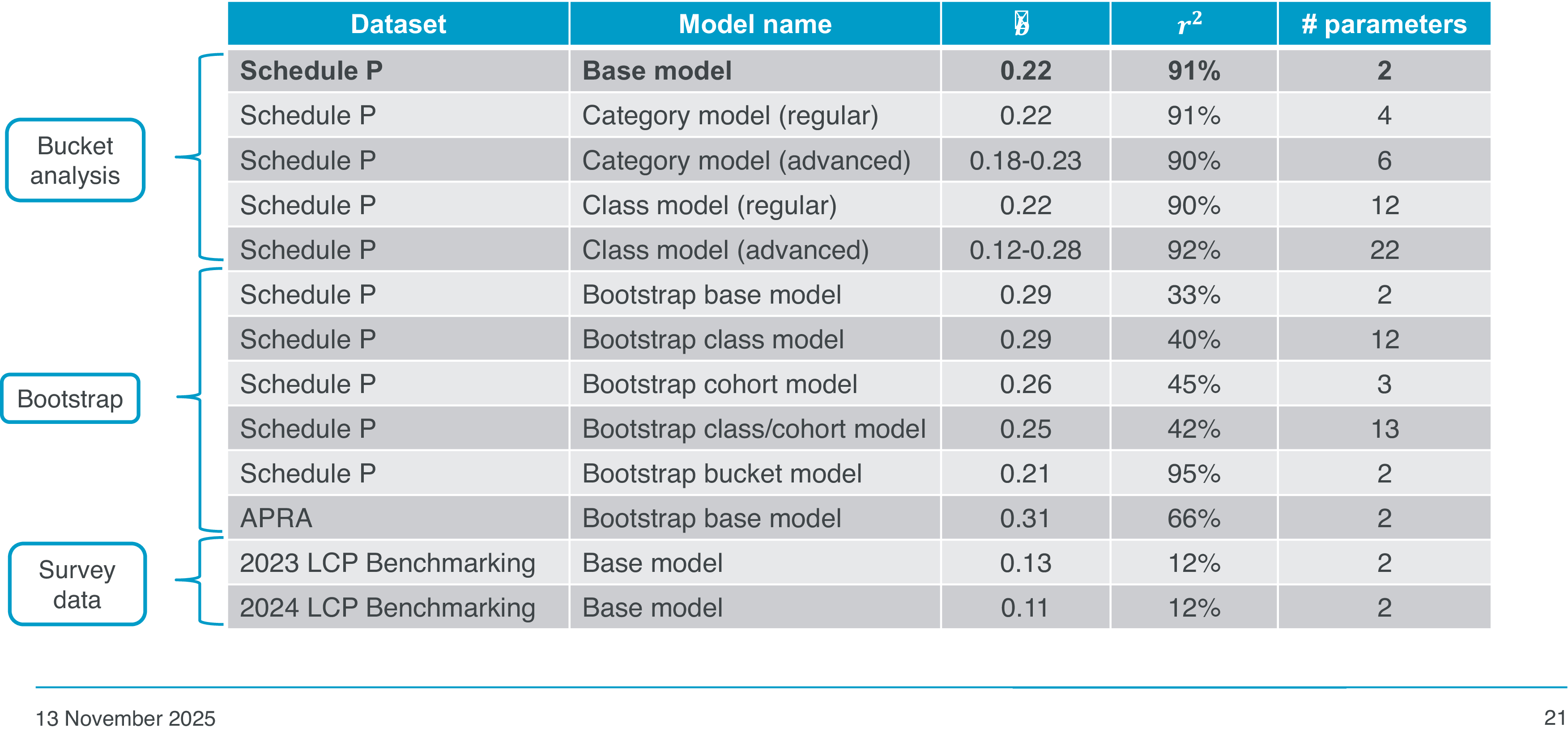
We did not just fit our base model. We looked at refining our model to include interactions for class and duration. That is what the four rows on the left-hand side of Figure 7 represent. In the table, the base model with the b parameter of 0.22 is in the first row. The second row has the parameters for a regular class model. For this model, instead of a universal a value, we let a vary across the classes of business. We kept the universal b value, so the gradient of the trend line is the same for each class of business, but they each have a different intercept. It is a more refined model. Looking at the results, the value for b is 0.22, which is consistent. The reason for looking into the additional models was to see if they were consistent with the base model. We are seeing that consistency. Again, the R-squared is 0.9, so model fit is good.

Figure 7.

Bucket analysis - granular level results.

In the third row is the advanced class model. For this model, we allowed different values for a and b. Instead of fitting one straight line, we now have a different straight line for each class of business because the intercept and the gradient vary. We calculated a range of b values, from 0.12 to 0.28. The central b value of 0.22 fits within that range. The R-squared value is a little bit lower for this model, at 0.6. The reason for that is that bucketing is quite a data-intensive process. With this model, we are sub-dividing that data set of 300 points into 12 classes. You are left with maybe tens of data points for each class that you are fitting this model to, which is not sufficient to have a very good R-squared metric.

The final two models are duration models. They are very similar to the regular and advanced class models, but instead of fitting to each class, we fit to each duration: short-tailed, medium-tailed, and long-tailed.

We also looked into the different b values that we calculated using the advanced class model, to see the impact of the class of business. The graph on the right-hand side of Figure 7 shows the different b values for the different classes of business from the advanced class model. In the paper we suggest that the b values change across the different classes of business with the level of systemic risk. We suggest that the five classes with the lowest b values are classes with lower systemic risk. It is difficult to prove this because it is a qualitative conjecture. You could try to find a quantitative metric that represents the degree of systemic risk for a class, but you might look at something like the sensitivity of diversification to volume, from which you could end up with the b value. It gets quite circular, and it is difficult to prove.

If you take auto physical damage, which has the lowest b value, as an example, what is going to cause a large reserve movement? Is it going to be large individual claims movements or something systemic like inflation? We think it is more likely to be something systemic, and as such we think that classes like auto physical damage, with lower b values, are more systemic. This is something that we want to try to expand on in the future.

We identified two main forms of uncertainty in the bucket analysis: parameter uncertainty and bucket uncertainty.

We have defined parameter uncertainty as the uncertainty in estimating our b parameter using a linear model. If you are fitting a statistical model to any data, you will get parameter uncertainty. As this is quite a well-known form of uncertainty, we can directly measure it by measuring the standard area of this parameter estimate b. This gives a value of 0.004, which as a proportion of 0.22 is very small. Therefore, we think that the materiality of this uncertainty is very low.

The second form of uncertainty that we identified is a little bit more nuanced. This is bucket uncertainty, and the graph in Figure 8 is illustrating this uncertainty. On the x-axis, the log of the reserve volume has been plotted. The reserve volume for each bucket was calculated as the average reserve size of the points in that bucket. Using the average size was somewhat arbitrary. We could have taken the median, the maximum, the minimum, and so on. The average reserve size has been used to determine the position of each blue dot in Figure 8, and any changes to those positions could potentially change the slope of the black line. We have defined bucket uncertainty as the uncertainty in quantifying reserve size for each bucket. Figure 8 has horizontal error bars on each of the blue dots to illustrate the range of reserve sizes within each bucket.

Figure 8.

Bucket analysis – uncertainty.

For a lot of the points the error bars are very small, but the bars on the right-hand side of the graph are visible. This highlights that we are seeing larger bucket uncertainty for the larger reserve sizes. This is because the data are sparse for large reserve volumes. We have much more data in Schedule P where the reserve volume is in the region of 10–100 million, compared to 50 billion. As the reserve size increases to this level, the buckets are having to become wider to contain 200 data points.

The paper contains more detail on the bucket uncertainty analysis. We ran a range of stability tests and showed that using different metrics, such as the median, maximum and minimum, instead of the average, barely changed the b parameter value. We are comfortable that the materiality of bucket uncertainty is low.

Miss J. Lagrue, A.I.A.: The next part of our analysis employed a bootstrapping technique to measure volatility. Bootstrapping is a resampling technique that we use to estimate the distribution of reserves from which a CoV can then be derived. We used an over-dispersed Poisson (ODP) bootstrap framework. This involved fitting a generalised linear model (GLM) with a log link function and an ODP area distribution to the incremental claims triangle. This process is the same as fitting a chain ladder to the triangle. The residuals are then calculated from the fitted model. We sampled with replacement the residuals to create a pseudo-triangle. The GLM is then refitted to the pseudo data set to produce a new estimate of the reserves, and this is repeated 10,000 times to derive a forecast output for each pseudo data set, which gives a distribution of reserve estimates. We had 9,403 claims triangles in the Schedule P data and we first filtered entities with greater than one million reserves just to provide some stability. That left us with 5,666 triangles to bootstrap. Each one of those triangles was bootstrapped with 10,000 simulations from which we then derived a CoV and a mean reserve for each cohort in the triangle.

Doing this meant that we could use the same data as Adam (Smylie) used in the bucket analysis, but with a very different technique to measure the volatility. However, the main reason to do this is that it is purely data-driven, so we do not have to rely on any judgement or actuarial estimates. As for all bootstrapping techniques, there are a number of well-known limitations including the fact that it is computationally intensive, especially when using this amount of data. Bootstrapping is also not guaranteed to converge to the true value. This is why we first filtered for entities with larger reserve sizes, to provide greater stability in the results. There are some additional limitations for this specific exercise. As I mentioned, this is a fully data-driven method. It is an automated approach on a lot of data, over 5,000 triangles. As a result, we are not applying any judgement. We did not do any smoothing of the data and we did not apply any tail factors. Schedule P is also market data, so some of the triangles are quite jumpy. One feature of the bootstrap is that if you get an unusual year of development, you can get a very high CoV.

After we had derived a CoV and a mean reserve for each cohort in the triangle, we took the logs of the CoVs and reserves and fitted a linear model. Figure 9 shows our base model, which is a linear model fitting the log CoVs to the log reserve volumes of our bootstrapping. That resulted in a b parameter estimate of 0.29. While the R-squared of this model is not great, at 33%, it is likely driven by those more sparse outliers that you can see in the chart. As I said earlier, due to the nature of the data, it is quite jumpy. When you run a bootstrap analysis on raw data, if you have spiky data, you can get very high CoVs and you would typically go and analyse those residuals. However, that just was not practical given the amount of data we were working with. Figure 9 also shows that the standard error of the b parameter estimate is very small at only 0.002, so there is very little uncertainty around that estimate.

Figure 9.

Bootstrapping analysis results.

As shown, we also fit a class model to the bootstrapping data, which improved the fit a little bit. We then fit a cohort model to see if the cohort had any effect, which it does not seem to have. The fit is a little better than the bootstrap base model and it reduced the b parameter slightly. Fitting a class and cohort model improved the fit again, and further reduced the b parameter estimate to 0.25. We used the same data but a very different technique and, whilst the fit of the model is lower than in Adam (Smylie)’s bucket analysis, the b parameter estimate for the base model is 0.29, which you can compare with Adam (Smylie)’s estimate of 0.22. Allowing for the outliers inherent in the data, and the bootstrapping method, you can see that trend line in the chart in Figure 9.

Next, we looked at combining bucketing and bootstrapping. We grouped the bootstrapping output into buckets by reserve size, and we again used buckets of size 200, to be consistent with the earlier analysis. We took the median log reserve and median log CoV for each bucket. We chose to use this median because the mean would have been skewed by those extreme outliers that we saw in Figure 9. Fitting this model resulted in a b parameter of 0.21, which is very close to our base model. Bucketing also improved the fit, achieving an R-squared of 95%. Along with simply reducing the noise in the data set, bucketing allowed us to effectively zoom out and get the bigger picture. It reduced the effect of other factors like class and cohort.

In Figure 10 we can see a levelling-off at those higher reserve sizes. This could be evidence of the undiversifiable volatility that we identified earlier. This minimum that we are seeing in Figure 10 works out to be a CoV of about 15.5%.

Figure 10.

Bucketing the bootstrapping results.

We also looked at the data from our LCP capital benchmarking survey. We collected data on reserve volumes and the actual selected CoVs for each respondent’s class of business. The data shown in Figure 11 is from our 2023 and 2024 surveys. The 2023 data is shown in blue, and the 2024 data is shown in pink. We have overlaid this benchmarking data against the raw unbucketed Schedule P data, which is shown in grey. By fitting a linear model to the 2024 benchmarking data, we obtained a b parameter of 0.11, and a similar result was obtained when fitting a model to the 2023 benchmarking data, with a b parameter of 0.13. These parameters are both lower than what we have seen so far. It is suggesting that actual selected CoVs are less sensitive to volume than we have seen in the other results. This can be seen in Figure 11, where the black line is the fitted model of the 2024 benchmarking data. It is much flatter than the dashed grey line of the bootstrapped base model. This is perhaps evidence of practitioners not taking volume sufficiently into account when selecting CoVs. You can also see in Figure 11 that the benchmark CoVs for smaller reserves are below the line, and the benchmark CoVs for very large reserves sit above this bootstrap baseline. This implies that the CoVs for smaller reserves are too low, whilst the CoVs for very large reserves are slightly too high. The break-even point where these two lines intercept suggests the average capital actuary’s mental reference point for volume is about 50 million, and that corresponds to a CoV of about 25%.

Figure 11.

LCP capital benchmarking survey.

We also looked at a different data set, the APRA data. This is much smaller than the Schedule P data, with total reserves of less than $50 billion (AUD). There are only 16 triangles in this data set, one for each class of business that is reported. We bootstrapped these triangles and took the logs of the CoVs and reserve volumes. As you can see in Figure 12, the data is much more sparse, but you can see a trend. This is confirmed by an R-squared of 66%, which is an improvement on the bootstrapped Schedule P model. It is interesting to note that the b value is higher for this data at 0.31, which suggests a greater sensitivity of volume on volatility for this APRA data. We have used a different technique and a different data set and found that the outcomes are reinforcing the results that we have already seen.

Figure 12.

Other market datasets: APRA.

Figure 13 shows a summary of the results. The key result is the base model result, which is on the actual historic reserve deteriorations. This model produced a really good fit and has amongst the fewest parameters. The bootstrapping then typically results in slightly higher estimates for b, which implies more sensitivity to volume in the triangles than in the actual selected reserves. However, this could largely be attributed to the data artefacts and would likely disappear if the trials were smoother and outliers were excluded. This was seen when we bucketed the bootstrap output. It improved the fit and also reduced the b parameter estimate to 0.21, which is more consistent with and very close to the 0.22 in the base model. The benchmarking data of actual selected CoVs suggests less sensitivity to volume than we have seen in the other results, which could be evidence of people perhaps not fully allowing for the effect of volume when parameterising CoVs.

Figure 13.

Summary of results.

Mr Gedalla: Bringing back the use cases or the case studies that we introduced right at the start of the presentation, we now have ways of adjusting reserve risk CoVs to allow for changes in reserve volume from year to year. We have a way of scaling down the volatility or scaling up the volatility of a market benchmark in order for it to be on a like-for-like comparison basis with selected CoVs for a given firm. We have a way for capital modellers to adjust the selected parameters in their model to take account of sensitivities or scenario testing, in particular looking at different business plan outcomes. We also have a way of scaling up the volatility for existing distributions to allow for additional volatility on smaller books.

In Figure 14, the impact on CoVs for some typical potential use cases is shown. It shows the impact and target CoV if you take a reference volume and reference CoV and scale that by an order of magnitude. For example, for a reference volume of 100, having a target volume of 10 increases the CoV from 30% up to just under 50%. That is a two-thirds increase. Conversely, increasing the target volume to 1,000 reduces the CoV by around 40%.

Figure 14.

Worked examples.

These are not huge adjustments. You might think that increasing the volume or reducing the volume by an order of magnitude would imply a very large impact on the volatility, but this is not the case. These are not the sort of assumptions that would break capital models. These are relatively minor adjustments that would result in sensible movements in overall capital. As shown in Figure 14, this method assumes that nothing is changing in the risk profile when the volumes change. We assume that the underlying nature of the reserves is the same, going from a reserve volume from one year to the next. These assumptions start to break down if we are talking about writing lots of different classes of business, or different claim types, that have not been included in the data before. We would suggest that this is used within the parameters that we are selecting here, in particular going up or down by an order of magnitude. The method will still work for larger movements, going from one million to 100 million for example. However, we do not recommend doing that. It is highly unlikely that volume will be the only change with that level of movement. It is quite likely that there will be some change in risk profile as well.

We have demonstrated that the power curve describes the relationship between reserve volume and reserve volatility well. Our suggested exponential parameter for b is 0.22 and that is supported by various approaches. However, we have uncovered some potential evidence of anchoring bias when practitioners select their reserve risk CoVs. In particular, CoVs for reserve volumes smaller than the tens of millions might well be overstated and CoVs for volumes greater than the tens of millions might be understated.

There are some possible refinements to the model that we would like to explore. We would like to understand the impact of class, for example why some classes seem to have different b parameters than others. Is that just pure random chance or is that something fundamental in the nature of those classes that is driving the difference? In particular, if we extended this analysis to underwriting risk, would we see similar class effects or does that balance between systemic and specific risk break down or possibly transform into something else when we look at claims that are in the future rather than in the past?

It would be good to understand how this works in different geographies. We have looked at the United States. We have verified to the best of our ability that Australia matches those results in the broad sense, but obviously more data and more results from different parts of the world would help support the core analysis.

Moderator (starting the Q&A session)

Mr J. M. Tomlin, F.I.A.: On the idea that there is more systemic risk in some classes than others, and that it might be an inflationary driver, for example. To what extent does your data set include economic inflationary shocks, for example? Is there potential value in looking to exclude those?

Mr Gedalla: The range of the data set ends in 2022 so possibly does not include the big inflationary spike that we saw in 2022/2023. We have not looked at the cohort effects by class in that degree of detail, and possibly you just start to get noise at that point. But it is certainly possible that inflation and similar drivers would be the reason for the different effects.

Mr E. Harrison, F.I.A.: What suggestions would you have for people who are interested in implementing this theory into their parameter setting processes? Specifically, what advice would you have around picking an appropriate b parameter for your company or portfolio, and then justifying that to validators later in the process?

Mr Smylie: Our suggestion would be to use the b value of 0.22. You could adjust that for class. We would need to do more research to be 100% sure that the level of systemic risk in a class does indeed lower the b value. We are broadly confident that the direction is correct, and that more systemic risk does imply a lower b value. Work is required to determine how much it lowers the b value. You could take a broad-brush approach if you know your class is quite systemic, for example motor. You could make a broad-brush adjustment to that 0.22 parameter with some expert judgement applied.

Question online: Are Ogden rate changes or other regulatory changes an example of non-diversifiable risk?

Mr Gedalla: They are in the sense that they are a one-off systemic shock. They will affect all blocks of business across the whole market and would also potentially affect lots of different claims within the same portfolio. The question is just about how much of a shock those are, to what extent they affect all claims, and whether it is on a size basis. Ogden, for example, would affect claims of a certain size and above. It would have much less of an effect on smaller claims. For regulatory changes, it is harder to see how that might impact a portfolio in that way. I guess we are thinking more about things like legal precedence. A change in a legal precedent that results in all claims in a portfolio going up would start to come through. We are looking at the overall relationship without thinking about individual events.

Mr Smylie: We did not see any evidence of undiversifiable volatility from the bucket analysis with Schedule P. However, the data set is only from 2010 to 2022, so we could do more analysis to see if there were any regulatory shocks in that time. It would be interesting to look at the systemic events that impacted the US over that time to see whether they came through in the data.

Mr Gedalla: I think that is something that is very much class specific. We are trying to come up with a parameter and a view for the whole market irrespective of class. There are going to be specific factors that affect individual classes of business and that is the sort of analysis that firms with sufficient data might want to look at.

Mr A. J. Newman, F.I.A.: You show in the paper, and you mentioned here, that a b value of 0.5 would be equivalent to all risks being independent. A b value of 0 would show all risks being dependent on each other. Have you considered what relationship between risks would be indicated by a b value of 0.22? For example, imagine company A and company B. Company B has reserves that are four times the size of company A’s reserves. You find that that is partly because of the number of risks it takes on – it takes on twice as many risks – and partly because of the line size that it is writing. It is writing lines that are twice as large, so it ends up with reserves of four times the size. Intuitively, that would give me a b value of something like 0.25. I wondered if you had thought about that sort of thing?

Mr Gedalla: We get a straight line when we plot this in log space. That is equivalent to saying that the effect is constant across all volumes. This implies that your hypothesis, which I agree is compelling intuitively, makes sense, but is not reflected in the data. There are various possible reasons for that. The key that it comes back to is that we are thinking very much about real-world applications. There are lots of academic type papers where it is useful to think about a sample portfolio that has a certain number of risks. It has assumptions, such as all or nothing loss, and various other assumptions that we do not see in the real world. We are focused on actual reserve movements that we see for reserve portfolios that exist. The data imply that everything cancels or there are enough other things going on that those types of relationships do not apply. We can resolve everything down to a single constant rate of change of volatility with volume.

Mr Smylie: Going into the research we expected a b parameter of 0.25 because we expected there to be some specific risks and some systemic risks. Therefore, it would be somewhere in-between 0 and 0.5, and the mid-point seemed reasonable.

Moderator: Have you had any feedback in terms of how people are using the results in practice?

Mr Gedalla: Various people have been in touch to say that this is useful. There are lots of other implementations of this relationship in the market. If you talk to capital modellers, lots of them will tell you that they have their own preferred way of making this adjustment. People have said that this is useful in parameterisation as a sense check on movement of numbers from year to year. If you have a CoV from last year, and you know that the reserve has moved in a particular direction since then, it provides a useful sense check on the new parameterised volatility. That is one example. Another example is in validation, and being able to sense check data against the market. You can look at market level statistics or published data from companies and then you are able to apply that to a like-for-like comparison point.

Mr Newman: You restricted your use cases to those in capital models. It strikes me that one very common use of a CoV and reserve relationship is in calculating the risk margin under Solvency II. This might be where you have a claims portfolio with risks paying off over time and you have to estimate what the solvency capital requirement is in future years. People are often doing that using a relationship such as this, so now they can move from b=0.25 to b=0.22.

Mr Gedalla: The risk margin is an interesting one and this has come up a few times. We have had some interesting conversations about it. The usual assumption for the risk margin run-off is the square root approach. That is effectively the key assumption that people use to simulate how future capital requirements evolve over time. The square root rule is obviously equivalent to the 0.5 b parameter that we showed being in fact the upper bound of the possible range of outcomes. The explanation is that the risk margin run-off is trying to do two things. It is firstly looking at the reduction in volumes as the capital runs off to ultimate, but it is also looking at the increase in certainty as claims start to be reported and settled and moved through that process. That is why it is a different assumption to the one that we have come up with and they do not contradict each other. If you look at it properly, the two support each other.

Moderator: A key part of the analysis you did was based on the Schedule P US data. What differences might you expect to see if the analysis had been run on UK data instead?

Mr Gedalla: I looked at UK data around ten years ago and managed to get the same result, or very similar results, between Schedule P and what used to be the Financial Services Authority (FSA) returns (previously the Department of Trade and Industry (DTI) returns). My understanding is that those returns are no longer available in a way that we can query. If anyone has the power to bring back those returns, that would be very much appreciated.

Moderator: Are there any extra considerations that people should be making to mitigate the reliance on industry data?

Mr Gedalla: With industry data there is the need to make sure that it is covered appropriately under Solvency II. The key element here is around sensitivity testing; to understand to what extent this parameter matters in the context of capital modelling. What we have found is that this is an assumption that can be systemic. For example, if it is used in the reserve risk process for calculating the final CoVs, that is potentially something that could affect every class. It might be something that moves every class in a particular direction, or there might be ups and downs, for example if it used as a way of moving from year to year in a steady state portfolio. You would not expect that to influence the results in any particular way. However, either way it should be straightforward to take a cut of the reserve risk process with a different value for b. If we take 0.22, then a sensitivity test might be, say, 0.18 or 0.3. My hope would be that there would not be a material impact on the overall Solvency Capital Requirement (SCR), but it would be great to hear from people who have managed to do that and have proven or disproven that hypothesis.

Mr T. G. Durkin, F.I.A.: I would love to hear a little bit more about the journey that you went on in terms of the parts of the research where you had eureka moments, and maybe the bits that were more frustrating?

Miss Lagrue: The start of the bootstrapping process was quite difficult. Trying to set up a process to bootstrap all those triangles was very difficult. Once we got that going it opened up a lot more data for us. One eureka moment was when we decided to look at bucketing the bootstrap output. When we had bucketed it and we saw the fit around the line and calculated the R-squared of 95%, it solidified the whole process. Seeing that element of levelling off that we expected from the undiversifiable volatility made us think it could be there, and it needs a bit more work to try and find what level it is at.

Mr Smylie: The bucket analysis was smooth. Seeing the results of the bucket and the bootstrap combination was a pretty special moment. It was one or two days before we were due to give the talk. Neil (Gedalla) was very adamant that we were not to do any more research, but we had this idea on the back of the bootstrap and it worked out quite nicely. We had a bit of a head scratch with the differences in b values across the classes of business. I think that is something that we would like to have a look at later.

Mr Gedalla: Referring back to Figure 11, this shows the relationship between what the data suggests and what practitioners actually choose. It shows that there is less sensitivity in the selections than there should be, or at least than the data implied that there should be. For me, that is great. It is something that is implied by the whole market rather than something that you can see in any one capital actuary’s selections or any one firm’s selections. As consultants, this is the sort of value that we can add – telling people that something is not quite stacking up that they would not necessarily be able to see for themselves.

Mr M. J. Botcherby, F.I.A.: When you presented the results from the Australia data set and the difference in the b value was shown as being closer to 0.5, my immediate reaction was that it is a feature of the very different population size and density. Had you given any thought to that and whether that would serve as a useful rule of thumb for each geography?

Mr Gedalla: It is potentially also a feature of a very different actuarial regime. Australian actuaries have different ways of thinking about things, in particular reserving. They tend to use more stochastic methods and they think more deeply about the range of possible outcomes from a given reserve. Another possibility is that it could just be noise. We are focusing on the relationship between the 0.31 from APRA and the 0.29 from the bootstrap-based model. Those are the two like-for-like comparison points and they are fairly close. With Schedule P we can do more with the data set because it is bigger – we are able to adjust that number down. They are quite close on a like-for-like basis. There are potentially a number of reasons why that might be.

Questioner: On the risk margin point, if you have got a specific run-off portfolio would you then be saying that your b factor should be much closer to 0.5?

Mr Gedalla: At one point the 0.22 is fine because in that data set there are portfolios that are new, in run-off, growing, shrinking, and so on. Once you get right into the tail of the run-off with the risk margins that assumption becomes inappropriate, because it is trying to simulate the change in capital. It is a change in underlying risk profile rather than just a pure volume change. In terms of going from, say, one year to the next, it is probably not enough of a factor to matter, but in terms of several years’ development, especially with short tail classes, then potentially, yes.

Mr Smylie: In the bucket analysis, when we were looking at the percentage reserve movements, we did not allow for run-off as volatility. If the reserve went from three million to one million over the calendar year because two million was paid, that was not considered as volatility. We would make sure to add back the paid amount. Effectively, we are looking at percentage movement as an ultimate.

Moderator: What is next in terms of building on this analysis and extrapolating it further? Are there any new areas that you are planning to look into?

Mr Gedalla: In terms of this piece, it is not closed. We have got to a good place where the results are reliable and can be used. As we mentioned, there are still some things to understand. We would be delighted to hear from other people who would like to pick up that challenge and try to explain what is going on or to replicate the results. We are looking to move into different areas. One of the things that we tried to do along the way was to look at the reserve risk CoV. What is intrinsically the reserve risk pattern that we see in the data? Dos that correspond to the lognormal distribution that firms typically choose? There were some challenges with doing that in this piece of work and in terms of scope we chose not to focus on that, but we are keen to pick that one back up.

Moderator: Thank you to everyone for participating in the discussion, and thank you very much to Neil (Gedalla), Jade (Lagrue) and Adam (Smylie).