1. Introduction
Nowadays, the rising demand for automation and robotics across different industries has highlighted the importance of online trajectory optimization in robotic and mechatronic systems [Reference Liu, Huang, Liu, Guo, Wang and Tan1–Reference Zhang, Zhou and Li3]. As these systems are increasingly employed in diverse manufacturing and robotic applications, there is a growing need for accurate dynamic modeling techniques and motion planning optimization to meet the demands of minimizing execution time and energy consumption [Reference Li, Lan, Jiang, Cao and Zhou4, Reference Clochiatti, Scalera, Boscariol and Gasparetto5]. For instance, approaches to minimize the energy consumption of robotic systems include the optimization of the parameters that define the robot trajectories [Reference Carabin and Scalera6, Reference Vanbecelaere, Van Oosterwyck, Derammelaere, Cuyt, Monte and Stockman7], the optimal positioning of the desired task within the robot workspace [Reference Vidussi, Boscariol, Scalera and Gasparetto8, Reference Fabris, Scalera and Gasparetto9], as well as the optimization of the configuration of modular robotic systems [Reference Althoff, Giusti, Liu and Pereira10]. Furthermore, the strategy proposed in ref. [Reference Shushtari, Nasiri, Yazdanpanah and Ahmadabadi11] leverages the optimal parallel compliant elements and the frequency of reference trajectories for energy efficiency in cyclic tasks, whereas in ref. [Reference Khoramshahi, Nasiri, Shushtari, Ijspeert and Ahmadabadi12] adaptive natural oscillator are considered to exploit natural dynamics for minimizing the energy consumption. In ref. [Reference Gadaleta, Pellicciari and Berselli13], the motion parameters of industrial robots are optimized for energy efficiency using a tool for automatic code generation. In ref. [Reference Liu, Huang, Liu, Guo, Wang and Tan1], a trajectory planning approach for large redundant manipulators is presented considering kinematic constraints and energy efficiency. Moreover, in ref. [Reference Ye, Hao and Cheng14] a multi-objective optimal trajectory planning strategy is described for robot manipulators considering traveling time, energy consumption, and joint jerk.
Among the multitude of robotic and mechatronic systems, those with a single degree of freedom (DOF) are extensively employed across various applications in production, packaging, and logistics facilities. In the literature, several studies that address the energy efficiency in 1-DOF systems can be found. For example, in ref. [Reference Wolf and Feenders15] energy efficient trajectories are investigated for flexible Variable Stiffness Actuators for robot joints. In [Reference Richiedei and Trevisani16], the authors present an analytical computation of the energy-efficient optimal planning in rest-to-rest motion of constant inertia systems. A derivation of the energy formulation for standard point-to-point trajectories, i.e., trapezoidal and cycloidal speed profiles, is presented in ref. [Reference Carabin and Scalera6] and applied to different mechatronic systems with 1 DOF. Furthermore, an analytical methodology to minimize the energy expenditure of mechatronic systems performing point-to-point trajectories based on trapezoidal, cycloidal, and polynomial trajectory motion primitives is developed and validated in ref. [Reference Carabin and Vidoni17]. In ref. [Reference Halinga, Nyobuya and Uchiyama18], an optimal motion planning approach is proposed for path and velocity optimization to achieve a trade-off between time and energy consumption in industrial machines. The authors in ref. [Reference Clemen and Rupp19] present a simple offline framework based on basic kinematic relationships to generate optimal motion trajectories for different performance objectives, including energy efficiency. Differently, in [Reference Maes, Yahya, Van Oosterwyck, Chevalier and Derammelaere20] a co-optimization approach is illustrated that integrates geometry and motion profile optimization in one architecture for energy-optimal point-to-point trajectories.
Nonetheless, only in few recent examples an online optimization is performed for energy efficiency. For instance, the authors in ref. [Reference Wang, Zhao, Bortoff and Ueda21] present a real-time algorithm capable of planning energy-optimal trajectories for a servomotor system subjected to acceleration and speed constraints in point-to-point motions. The algorithm divides the trajectory in different sections (e.g., speed- and acceleration-constrained phases) and optimizes the execution times of the various sections with a fixed total time. Furthermore, in ref. [Reference Donà, Lenzo, Boscariol and Rosati22] a method is proposed for real-time planning of minimum-energy trajectories for servo-actuated systems that exploits the optimization of the trajectory parameters. However, in these last two examples, the total time is fixed and only the shape of the trajectory is optimized for energy efficiency, without considering the variation of the execution time. Nevertheless, modern production systems require flexibility and real-time adaptability as they are often employed in complex and dynamic environments. Therefore, systems capable of online trajectory optimization that consider both execution time and energy consumption are needed.
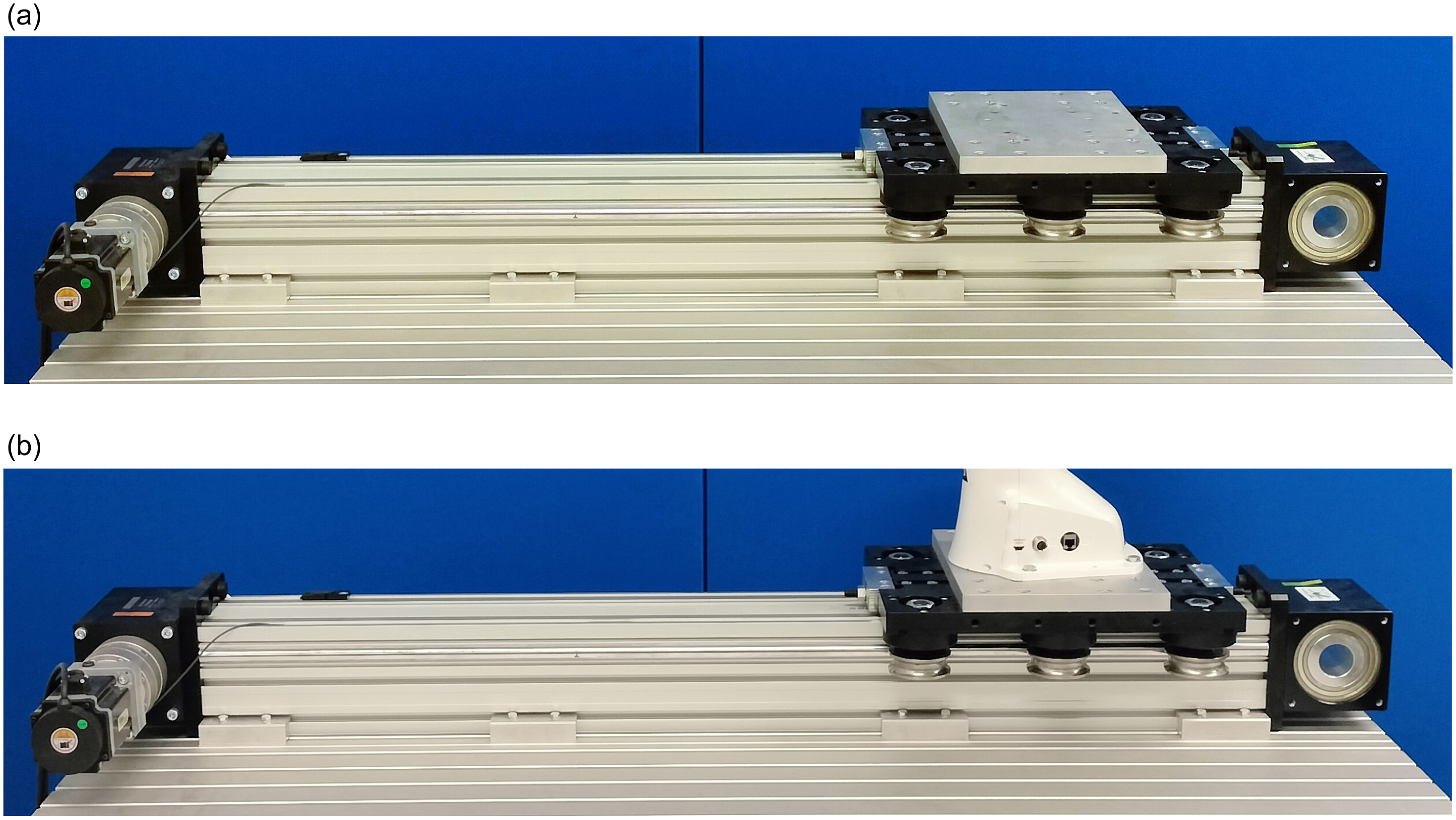
In this work, we present an approach for the online optimization and planning of minimum-time and minimum-time-energy trajectories for a 1-DOF linear axis (Figure 1). The online optimization is based on a verified dynamic model of a belt-driven system that also includes an accurate friction model retrieved through the identification of optimal friction parameters. Extensive experimental results highlight the capabilities of the proposed approach in optimizing online the point-to-point motions of the cart of the linear axis, minimizing the execution time and the energy consumption, and allowing the execution of sequential optimal motions without idle times. Furthermore, the experimental results are also analyzed in terms of computational times to evaluate the performance of the online trajectory optimization strategy.
Robotic linear axis without payload (a) and with payload (b).

This paper extends our previous work in ref. [Reference Fabris, Scalera and Gasparetto23] including novel contributions that allow us to (i) further analyze the friction effects in the linear axis; (ii) evaluate the computational times for the online optimization of the point-to-point trajectories in different scenarios and with different open-source optimization tools; (iii) analyze the performance of the online optimization with different dynamic conditions of the system, i.e., without payload (Figure 1a) and with payload (Figure 1b).
To summarize, the key contributions of this paper are the following:
-
• an approach for the online optimization and planning of minimum-time and minimum-time-energy point-to-point trajectories in 1-DOF robotic systems;
-
• the dynamic modeling and identification of friction parameters of a 1-DOF linear axis, by also comparing different friction models to describe friction behavior;
-
• a comparison of the performance of three different open-source optimization tools to select the most suitable for the online solution of the optimization problems in terms of computational times;
-
• the results of extensive experiments on a linear axis to evaluate the performance of the proposed approach in terms of energy efficiency, traveling time, and computational time.
The proposed optimization approach is general and can be applied to similar systems with 1 DOF that can be steered using custom trajectories, and that make available joint position, velocity, and torque signals. Furthermore, the approach can be easily extended to robotic systems with more than one actuator to plan optimal minimum-time and energy-efficient trajectories in more challenging scenarios.
The paper is organized as follows: the proposed online optimization and trajectory planning approach is described in Section 2, whereas Section 3 illustrates the dynamic modeling and friction parameters identification of the considered 1-DOF linear axis. Section 4 describes the experimental setup, and the experimental results are analyzed and discussed in Section 5. Finally, Section 6 concludes the work and provides possible future developments.
2. Optimization of minimum-time and minimum-energy trajectories
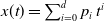
The online optimization of point-to-point trajectories for the robotic linear axis considered in this work is performed by using polynomial motion laws of degree
 $d$
equal to 3, 5, and 7 (poly3, poly5, poly7), i.e.,
 $x(t)=\sum _{i=0}^d p_i\, t^i$
, where
 $p_i$
represents the i-th coefficient. The execution time for the generic trajectory from an initial point to a final point is defined as
 $\Delta t = t_f-t_i$
. The constraints for the poly3 motion law are
 $x(t_i)=x_i$
,
 $x(t_f)=x_f$
,
 $\dot {x}(t_i)=0$
, and
 $\dot {x}(t_f)=0$
. In the poly5 trajectory, the constraints
 $\ddot {x}(t_i)=0$
and
 $\ddot {x}(t_f)=0$
are also considered. In addition to the previous ones, for the poly7 motion law
 $\dddot {x}(t_i)=0$
and
 $\dddot {x}(t_f)=0$
are also imposed. The optimization problem that is solved online aims at finding the optimal execution time of the point-to-point motions for two different approaches that can be formulated as follows:
-
• Approach (1): minimum-time optimization:
(1) \begin{equation} \underset {t}{\text{min}} \quad w_0 \, t \end{equation}
-
• Approach (2): minimum-time-energy optimization:
(2)
\begin{equation} \underset {t}{\text{min}} \quad \omega \,t + (1-\omega )\,E \;\;\; \text{where} \;\;\; E = \int _0^t \mid \boldsymbol{F}\, \boldsymbol{\dot {x}} \mid \, {\rm d}t \end{equation}


In both approaches, the optimization problem is subjected to the following constraints:
 \begin{equation} \left . \begin{cases} x_{{lim}^-}\lt \boldsymbol{x}\lt x_{{lim}^+} \\ \mid \boldsymbol{\dot {x}} \mid \lt \dot {x}_{{lim}} \\ \mid \boldsymbol{\ddot {x}} \mid \lt \ddot {x}_{{lim}} \\ \mid \boldsymbol{\tau _m} \mid \lt \tau _{m,{lim}} \end{cases} \right . \begin{aligned} x_{{lim}^-}, x_{{lim}^+} \text{ lower and upper position limits} \\ \dot {x}_{{lim}} \text{ velocity limit} \\ \ddot {x}_{{lim}} \text{ acceleration limit} \\ \tau _{m,{lim}} \text{ motor torque limit} \end{aligned} \end{equation}
Approach (1) aims at finding the minimum execution time
 $t$
that does not exceed the constraints of the linear axis (Eq. (1)).
 $w_0$
is a positive weight used to improve the convergence of the optimization. Differently, Approach (2) optimizes the time that minimizes the weighted sum of time
 $t$
and mechanical energy
 $E$
(Eq. (2)). The total mechanical energy
 $E$
consumed by the robot during a trajectory is computed by integrating the absolute value of the mechanical power
 $\boldsymbol{P_i} = \boldsymbol{F}\, \boldsymbol{\dot {x}}$
over the execution time
 $t$
, as in Eq. (2). Therefore,
 $E$
corresponds to the mechanical energy that the robotic system requires to successfully complete the desired trajectory, considering both the energy needed for accelerating and braking the robotic system. The trade-off between the two contributions of the optimization problem for Approach (2) is set by means of the parameter
 $\omega \in [0, \,1]$
. The proposed approach is based on the minimization of the mechanical energy of the system. However, this strategy can be extended by considering a more comprehensive electro-mechanical model of the system in order to take into account also the losses in the electrical part (e.g., Joule losses, iron losses, stray losses), as in ref. [Reference Richiedei and Trevisani16].
To evaluate the performance of the considered approaches for the online trajectory optimization under variable dynamic conditions, two different cases are taken into account:
-
• No Payload: no payload is present on the cart of the linear axis (Figure 1a);
-
• With Payload: a payload is attached on the cart of the linear axis; in particular, the payload is given by a robotic arm with
$m_{{\rm load}} = 17.8\,{\rm kg}$
(Figure 1b).

The procedure for the computation of the motor torque
 $\boldsymbol{\tau _{m}}$
needed to steer the cart of the axis, and the approach for the identification of the friction parameters are described in Section 3.
3. Dynamic modeling and friction parameters identification
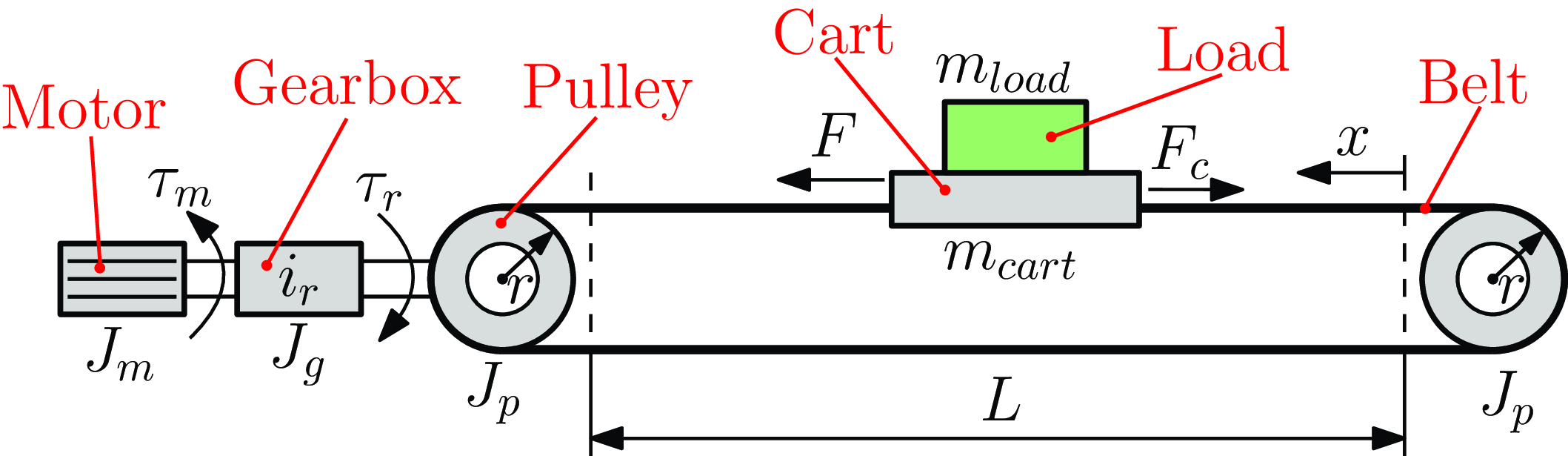
In this work, we consider a robotic linear axis with 1 DOF. The graphical model of the system is shown in Figure 2. The dynamic model of the axis can be formulated as follows:
 \begin{equation} \boldsymbol{F} = \bigg [m_{{\rm cart}} + m_{{\rm load}} + \frac {(J_{m}+J_{g}) \, {i_{r}}^2 + 2 J_{p}}{r^2} \bigg ]\, \boldsymbol{\ddot {x}} + \boldsymbol{F_c} \end{equation}
where
 $\boldsymbol{F}$
is the traction force acting on the cart,
 $\boldsymbol{\ddot {x}}$
is the linear acceleration of the cart, whereas
 $\boldsymbol{F_c}$
represents the friction force. Furthermore,
 $m_{{\rm cart}}$
indicates the cart mass,
 $m_{{\rm load}}$
is the mass of a possible payload placed on the cart, whereas
 $J_m$
,
 $J_g$
, and
 $J_p$
represent the motor, gearbox, and pulley inertia, respectively. The torque
 $\boldsymbol{\tau _m}$
needed by the motor to steer the cart along the desired trajectory
 $\boldsymbol{{x}},\boldsymbol{\dot {x}},\boldsymbol{\ddot {x}}$
can be computed from the force
 $\boldsymbol{F}$
, the gear ratio
 $i_{r}$
, and the pulley radius
 $r$
, as:
 \begin{equation} \boldsymbol{\tau _m} = \frac {\boldsymbol{F}\, r}{i_{r}} \end{equation}
Model of the robotic linear axis considered in this work.

In the considered dynamic model, the elasticity of the belt is neglected. The geometrical and dynamical parameters of the linear axis are assumed to be well known and are reported in Table I.
Geometrical and dynamical parameters of the linear axis.

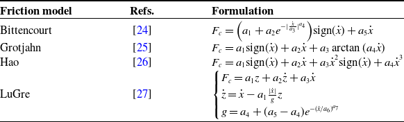
To accurately describe the friction behavior in the robotic linear axis, the Bittencourt [Reference Bittencourt and Gunnarsson24], Grotjahn [Reference Grotjahn, Daemi and Heimann25], and Hao [Reference Hao, Pagani, Beschi and Legnani26] static friction models, and the LuGre dynamic friction model [Reference De Wit, Olsson, Astrom and Lischinsky27] are considered. The mathematical formulations of the considered friction models are reported in Table II. Alternative friction formulations can also be taken into account, as for instance, those reported in refs. [Reference Fabris, Scalera, Boscariol and Gasparetto28, Reference Luo, Yuan, Hu, Du, Bao and Zhou29]. The friction models considered in this work only account for velocity-related terms. However, the actual friction is influenced by velocity, load, and temperature. To include the effects of load and temperature on the friction behavior in a more complete friction formulation, experimental data are needed where these parameters are varied over a wide range. In this way, the two different cases taken into account in this paper (loaded and unloaded conditions) could be considered in a single formulation. This can be useful when the loading conditions of the robotic system change frequently over time. Nevertheless, the generalization of a friction formulation in different loading scenarios is beyond the scope of this work.
Mathematical formulation of the friction models considered in this paper.
 $\boldsymbol{F_c}$
is the theoretical friction force computed by the friction models,
 $\boldsymbol{\dot {x}}$
is the cart velocity, whereas
 $a_j$
(
 $j=1,\ldots ,7$
) represents each of the friction parameters that are optimized to fit the dynamic model with the experimental data.

The considered friction models describe the friction behavior in different ways and using different mathematical formulations (Table II). All the three considered static friction models include a constant directional term to consider the Coulomb friction, and a velocity-proportional term to take the viscous friction into account. The difference between the models lies in how they model friction at low velocities. In the Bittencourt model, friction at low velocities is considered through a decreasing exponential function. The Grotjahn model includes a term proportional to the arctangent (arctan) of the velocity, whereas the Hao model adopts a third-degree polynomial formulation. Differently from the static friction models, which consider only the current state of the system and not its history, the dynamic friction models, including the LuGre one, comprise the state variable
 $z$
that also takes into account the history of the system. The dynamic friction models are better able to model friction at rest state and very low velocities rather than the static ones, but they require larger computational times due to the higher number of parameters and their differential formulation. Therefore, for online optimization purposes, a trade-off between precise friction computation and short calculation times has to be found.
For the identification of friction parameters, a proper excitation trajectory is designed, as in Eq. (6):
 \begin{equation} x(t)=\sum _{i} A_{1}\cos (2\pi f_i t) + \sum _{j} A_j\cos (2\pi f_{1} t) + \sum _{k} A_{2}\cos (2\pi f_k t) + \sum _{m} A_m\cos (2\pi f_{2} t) \end{equation}
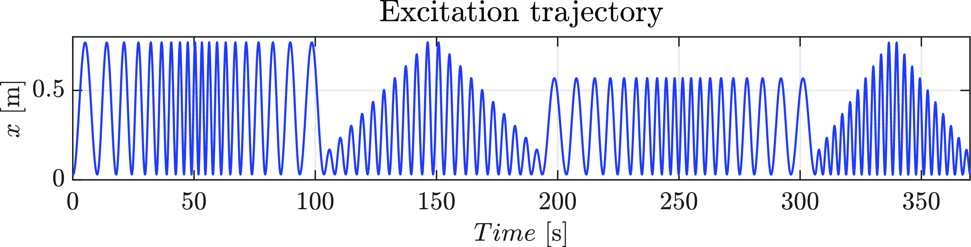
The excitation trajectory consists of a sinusoidal trajectory composed of four different sections: two with variable frequency
 $f$
and fixed amplitude
 $A$
(the first and the third ones), and two with variable amplitude
 $A$
and fixed frequency
 $f$
(the second and the fourth ones). This excitation trajectory is chosen since it enables a reliable friction modeling by exploring a wide range of cart velocities and accelerations. For each of the considered friction models, the optimal friction parameters are derived by minimizing the error between the motor torque computed with the dynamic model and the experimental one.
4. Experimental setup
The proposed online optimization approach is validated on a robotic linear axis by AutomationWare available at the Robotics and Mechatronics Laboratory at the University of Udine (Italy), shown in Figure 1. The linear axis employs a toothed belt made of polyurethane with steel strands. The system is actuated by a brushless motor HDT SR08L, connected to the driven pulley of the linear axis through a planetary gearbox with a reduction ratio
 $i_r$
equal to 10. The system does not provide the position of the cart with respect to a fixed reference frame using external sensors, but only through the angular position of the driven pulley, retrieved from the encoder mounted on the motor.
The maximum displacement
 $L$
of the cart is equal to 0.8 m. The geometrical and dynamical parameters used in the model of the system are reported in Table I. The friction parameters are optimized by adopting the constrained nonlinear multivariable Matlab function fmincon and the sequential quadratic programming (SQP) method. The system is controlled by means of a computer equipped with 32 GB of RAM and an Intel Core i9 processor running Ubuntu 20.04, using ROS 2 (Robot Operating System) Galactic Geochelone with Python 3.8. A sampling rate of 1 kHz is used for both the input trajectories and the measured cart position and velocity, and motor torque data acquired in ROS 2. The motor torque signal available in ROS 2 is measured directly from the servo drive readings. However, no data on the electrical currents and voltages of the actuation system are available from the ROS controller of the linear axis. For this reason, the optimization of the point-to-point trajectories for Approach (2) is based on a mechanical model of the system that accounts for friction and inertial contributions, which can be validated with the available experimental data.
To select the optimization algorithm most suitable for the online solution of the problems addressed in this paper, a comparison of the performance in terms of computational times of three different optimization tools is performed. In particular, we consider the IPOPT algorithm of CasADi [Reference Andersson, Gillis, Horn, Rawlings and Diehl30], the IPOPT algorithm by Pyomo [Reference Bynum, Hackebeil, Hart, Laird, Nicholson, Siirola, Watson and Woodruff31, Reference Hart, Watson and Woodruff32], and the SLSQP method by SciPy. CasADi is an open-source tool for nonlinear optimization, that facilitates rapid and efficient implementation of different methods for numerical optimal control. Pyomo is a Python-based open-source software package that includes many functionalities for formulating, solving, and analyzing optimization models. Moreover, SciPy is one of the most common open-source tools for Python, providing algorithms for optimization, integration, differential equations, and many other problems. Regarding the considered optimization algorithms, the IPOPT algorithm implements a primal-dual interior point method, using line searches based on Filter methods, whereas SLSQP is an SQP method. Following the comparison results shown in Section 5.2, to solve online the optimization problems in (1) and (2) with (3) we chose the IPOPT algorithm of CasADi.
For Approach (1), the lower and upper bounds for the time duration of each robot trajectory are
 $0.3$
and
 $3\,{\rm s}$
, respectively, whereas for Approach (2) they are set equal to
 $0.5$
and
 $20\,{\rm s}$
, respectively. Furthermore, the value of the parameter
 $\omega$
for Approach (2) is chosen equal to 0.9, to give more weight to the time reduction with respect to energy. The optimization algorithm is tested by planning point-to-point optimal motions through 100 random waypoints within the joint position bounds. We use the same waypoints for both minimum-time and minimum-energy trajectories and for each of the considered motion laws. The optimization process is performed in parallel with the trajectory execution, i.e., while the linear axis executes a point-to-point motion, the optimization algorithm computes the optimal time and plans the trajectory for the next motion. This parallel procedure allows the execution of one trajectory right after the previous one, without idle times.
Cart position
 $x$
for the excitation trajectory designed for both cases with and without payload.

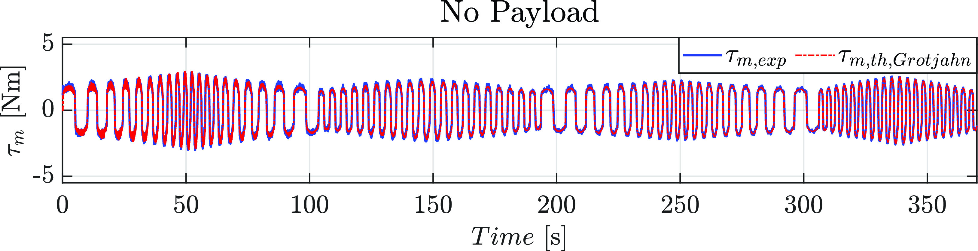
Experimental motor torque
 $\tau _{m,{\rm exp}}$
, and motor torque
 $\tau _{m,{\rm th},{\rm Grotjahn}}$
computed with the dynamic model for the excitation trajectory designed for the case without payload.

5. Experimental results
In this section, we illustrate the experimental results obtained for the friction identification procedure and for the online optimization approach. In Section 5.1, the performance of the considered friction models in describing the friction behavior and the computational times required to compute the optimal solution are presented, for both the cases with and without payload. Then, Section 5.2 outlines the experimental results of the online optimization approach, for both cases, both approaches, and each of the considered motion laws.
5.1. Results of the friction identification procedure
Figure 3 shows the excitation trajectory designed for deriving the optimal friction parameters for the case without payload, and Figure 4 shows the experimental motor torque
 $\tau _{m,{\rm exp}}$
, and the motor torque
 $\tau _{m,{\rm th},{\rm Grotjahn}}$
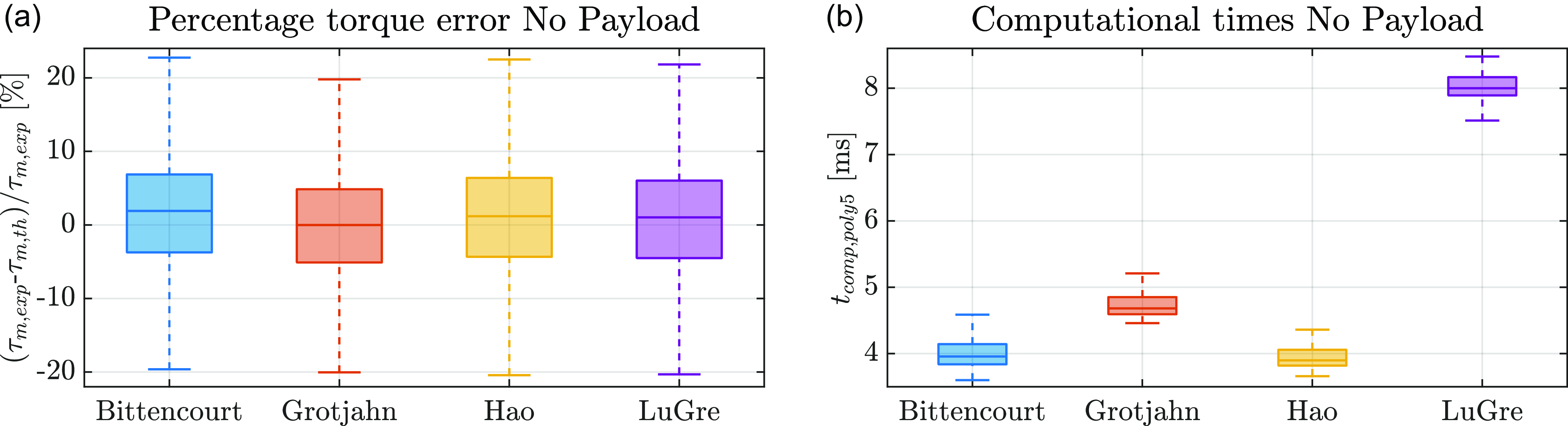
computed with the dynamic model (using the Grotjahn friction model) for the same case. Moreover, Figure 5a reports the box plot representation of the percentage error in computing the motor torque including the considered friction models in the dynamic model of the linear axis. In the box plots, the central line indicates the median, the bottom and top of each box represent the first and third quartiles, whereas the whiskers extend to the most extreme data points not considered outliers. From Figure 5a, it can be seen that the percentage torque error of the considered friction models is comparable and generally lower than 10%, with a smaller torque error obtained with the Grotjahn and LuGre models. Moreover, Figure 5b shows the box plot representation of the computational times required for calculating the optimal solution including the considered friction models into the dynamic model (the same exemplary trajectory planned with a poly5 motion law and a distance equal to
 $0.6\,m$
is computed 100 times for statistical purposes). From the box plots, it can be seen that the performance of the trajectory optimization changes with the considered friction models due to the different mathematical formulations. More in detail, the dynamic friction model (i.e., LuGre) is slower than the static ones (i.e., Bittencourt, Grotjahn, and Hao) due to the higher number of parameters and its differential mathematical formulation, which is more computationally demanding than the compact formulation of static models. As it can be seen from Figure 5b, with the LuGre model the online optimization approach requires about
 $8\,{\rm ms}$
to compute the optimal solution, which is about twice as much as that taken with static friction models. Therefore, for the dynamic model of the linear axis we take into account the Grotjahn model, which has the best trade-off between torque error and computational time. As it can be seen from Figure 5a and b, including the Grotjahn model in the dynamic model of the linear axis (Eq. (4)) results in maximum percentage torque errors generally lower than 10% and computation times of about
 $4.5\,{\rm ms}$
.
Box plot representation of the errors in the torque computation adopting the considered friction models for the case without payload (a); box plot representation of the computational times required for calculating the optimal solution including the considered friction models into the dynamic model, for the case without payload, the minimum-time approach, and the poly5 motion law (b).

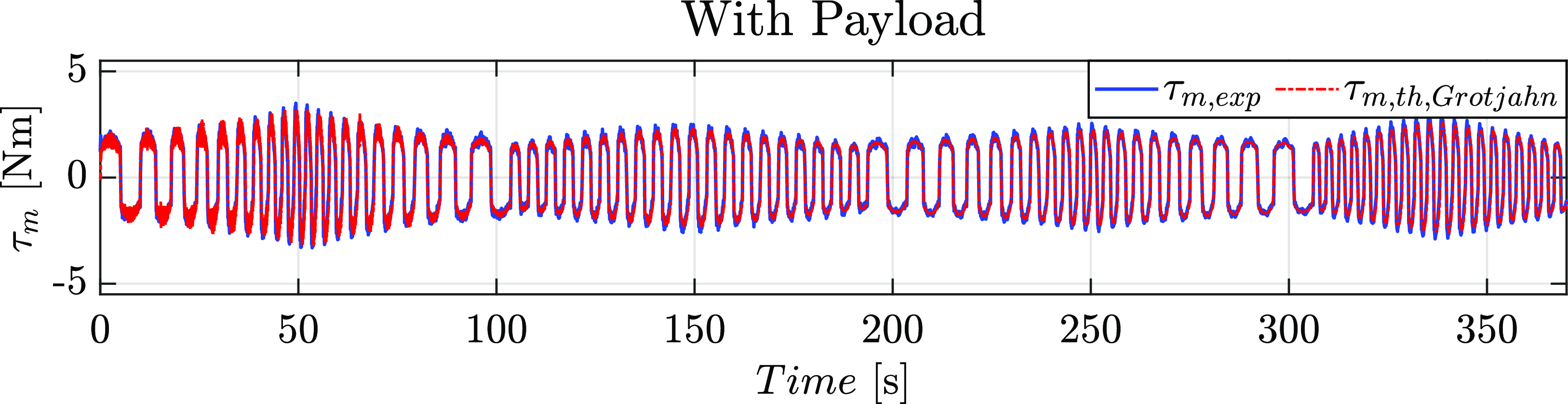
Experimental motor torque
 $\tau _{m,{\rm exp}}$
, and motor torque
 $\tau _{m,{\rm th},{\rm Grotjahn}}$
computed with the dynamic model for the excitation trajectory adopted for the case with payload.

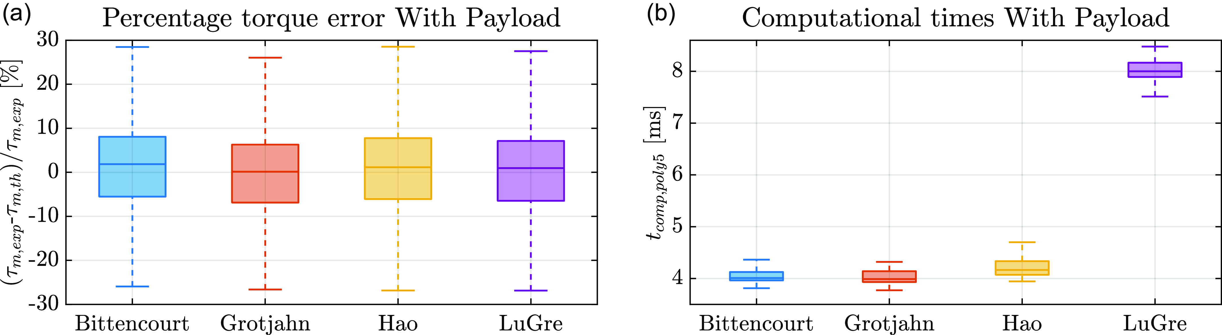
Box plot representation of the errors in the torque computation adopting the considered friction models for the case with payload (a); box plot representation of the computational times required for calculating the optimal solution including the considered friction models into the dynamic model, for the case with payload, the minimum-time approach, and the poly5 motion law (b).

Figure 6 shows the experimental motor torque
 $\tau _{m,{\rm exp}}$
, and the motor torque
 $\tau _{m,{\rm th},{\rm Grotjahn}}$
computed with the dynamic model for the case with payload, obtained using the excitation trajectory of Figure 3. Furthermore, Figure 7a shows the box plot representation of the percentage error in computing the motor torque when including the considered friction models in the dynamic model of the robotic system, highlighting a good and comparable accuracy of the compared friction models. Figure 7b reports the box plots of the computational times needed to calculate the optimal solution including the considered friction models into the dynamic model (the same exemplary trajectory planned with a poly5 motion law and a distance equal to
 $0.6\,{\rm m}$
is computed 100 times for statical purposes). As for the case without payload, in the case with payload the Grotjahn and LuGre models are the ones that exhibit the lowest torque error. Also in this case, the online optimization process takes about
 $8\,{\rm ms}$
to compute the optimal solution when adopting the LuGre model, i.e., twice the computation time required when static friction models are considered, due to the more demanding differential formulation of the LuGre dynamic friction model. Therefore, also for the case with payload the Grotjahn model is chosen to be included in the dynamic model of the linear axis (Eq. (4)), since also in this case it offers the best compromise between torque computation accuracy and computation times, with maximum percentage errors lower than 10% and computation times of about
 $4\,ms$
, as it can be seen from Figure 7a and b.
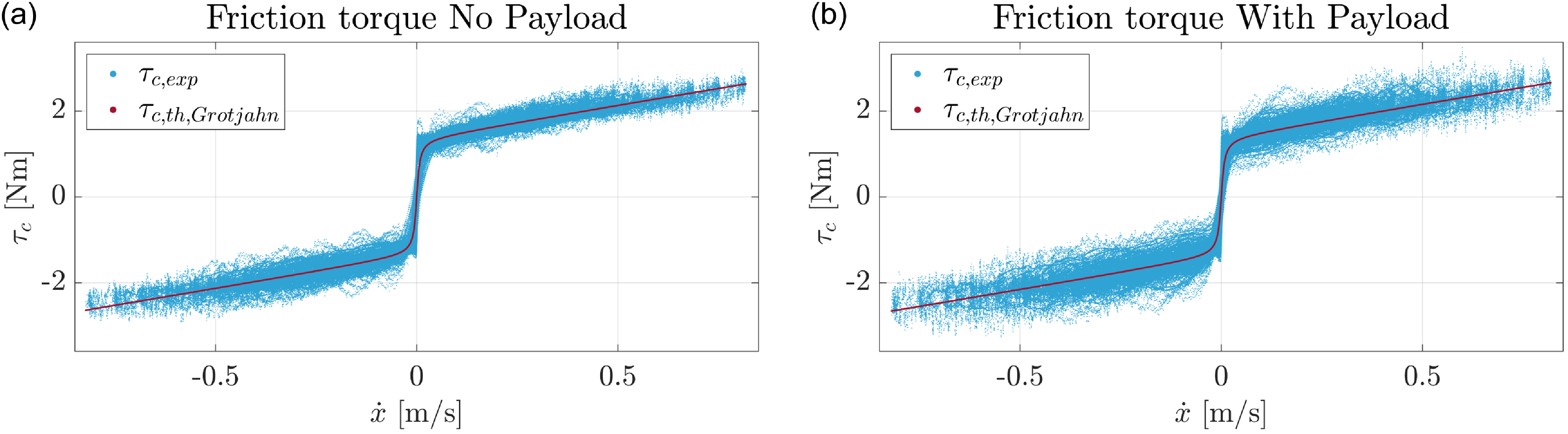
Figure 8 shows the comparison between the experimental friction torque
 $\tau _{c,exp}$
and the theoretical one obtained with the Grotjahn model
 $\tau _{c,th,Grotjahn}$
, for both cases. For the sake of clarity,
 $\tau _{c,exp}$
is obtained as difference between the experimental motor torque
 $\tau _{m,exp}$
and the torque not related to friction computed with the dynamic model
 $\tau _{dyn}$
(i.e.,
 $\tau _{dyn}=(F_{th}-F_{c,th})\, r/i_r$
), whereas
 $\tau _{c,th,Grotjahn} = (F_{c,th,Grotjahn}\,r)/i_r$
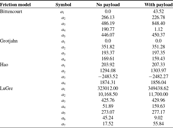
. Finally, Table III reports the optimal friction parameters obtained for the different considered friction models and for both cases. From Table III, it can be seen that some friction parameters, especially in the Bittencourt and LuGre models, change consistently from the case without payload to the case with payload, probably due to the high load considered for the second case, but generally the values of the friction parameters are quite close between the two cases.
Comparison between the friction torques
 $\tau _c$
over cart velocity
 $\dot {x}$
considering the data obtained with the Grotjahn model and the experimental data, for the cases without payload (a) and with payload (b).


5.2. Results of the online optimization approach
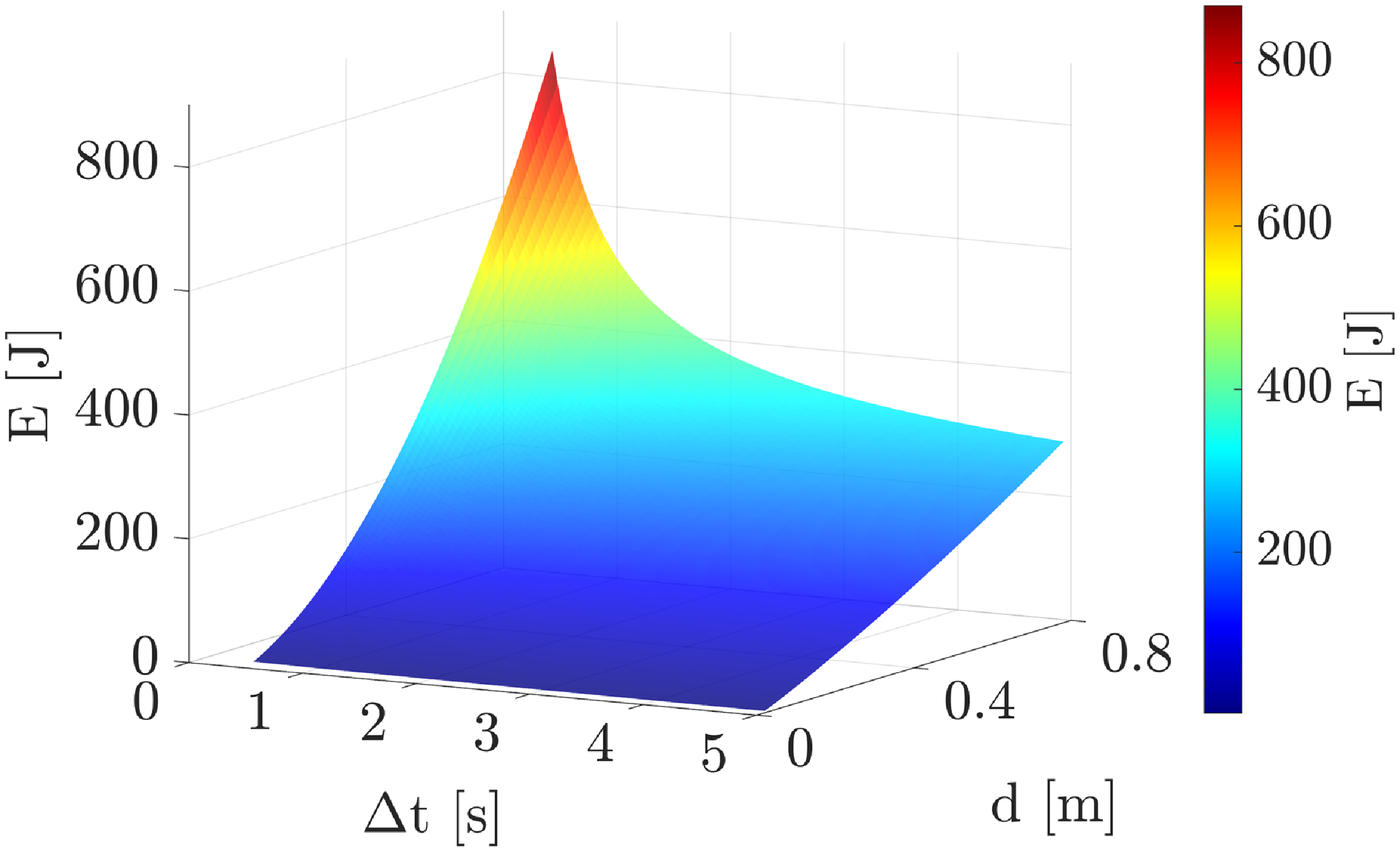
Figure 9 shows the 3D representation of the mechanical energy
 $E$
consumed by the robotic system during a poly5 trajectory as a function of traveled distance
 $d$
and execution time
 $\Delta t$
. In this figure, the mechanical energy
 $E$
is obtained from numerical simulations using the dynamic model in Eq. (4) for the torque computation, and each point on the graph considers only one point-to-point motion. The trend of the energy consumption as a function of the execution time and the distance is similar for the two cases, with slightly more energy required for the case with payload on the cart with respect to the other one for the same execution time and distance. This little difference is due to the fact that in the two cases the friction parameters are very similar (friction is the main torque contribution in the considered robotic system), and it is related to the added payload. For instance, for a traveled distance of
 $0.4\,{\rm m}$
and an execution time of
 $3\,{\rm s}$
, the consumed energy is equal to
 $145.09\,{\rm J}$
without payload, whereas it is equal to
 $147.28\,{\rm J}$
in the case with payload. For this reason, only the graph for the case without payload is reported. For execution times greater than
 $3\,{\rm s}$
, the mechanical energy expenditure increases approximately linearly with the traveled distance. Instead, for lower execution times, the energy consumption increases faster with the traveled distance. A similar behavior of the consumed mechanical energy trend can be seen by fixing the traveled distance. In particular, for traveled distances higher than
 $0.4\,{\rm m}$
, the mechanical energy consumption increases approximately linearly by decreasing the execution time until about
 $3\,{\rm s}$
. For lower execution times, the energy consumption increases faster with the decrease of the execution time. Moreover, the results shown in Figure 9 underline the importance of a proper selection of the execution time of the point-to-point motion in order to decrease the energy expenditure and find the best trade-off between cycle time, which is related to productivity, and consumed energy.
Mechanical energy as a function of traveled distance and total time for the case of poly5 trajectories, for the case without payload, obtained from numerical simulations.

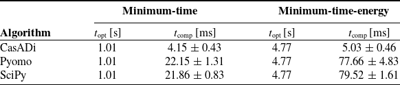
Table IV reports the comparison results for the choice of the optimization algorithm most suitable for the online solution of the problems addressed in this paper. The IPOPT algorithm of CasADi, the IPOPT algorithm by Pyomo, and the SLSQP algorithm by SciPy are compared in terms of optimal execution time
 $t_{{\rm opt}}$
and computational times
 $t_{{\rm comp}}$
, using the same poly5 trajectory that is optimized 100 times for a distance equal to
 $0.6\,{\rm m}$
. As it can be seen from the table, the three considered optimization algorithms found the same solution for both problems (i.e., the optimal time is equal to
 $1.01\,{\rm s}$
for the minimum-time optimization, and it is equal to
 $4.77\,{\rm s}$
for the minimum-time-energy case). However, the IPOPT algorithm of CasADi is significantly faster with respect to the compared optimization algorithms. Indeed, it requires about 80% less computational time for the minimum-time approach and about 90% less computational time for the minimum-time energy case than the other two considered algorithms. These results highlight that the IPOPT algorithm of CasADi is the most suitable for online optimization with respect to the compared optimization tools in the test cases considered in this work.
Comparison results for the choice of the optimization algorithm. The results are reported in terms of mean
 $\pm$
standard deviation for 100 optimizations of the same trajectory.

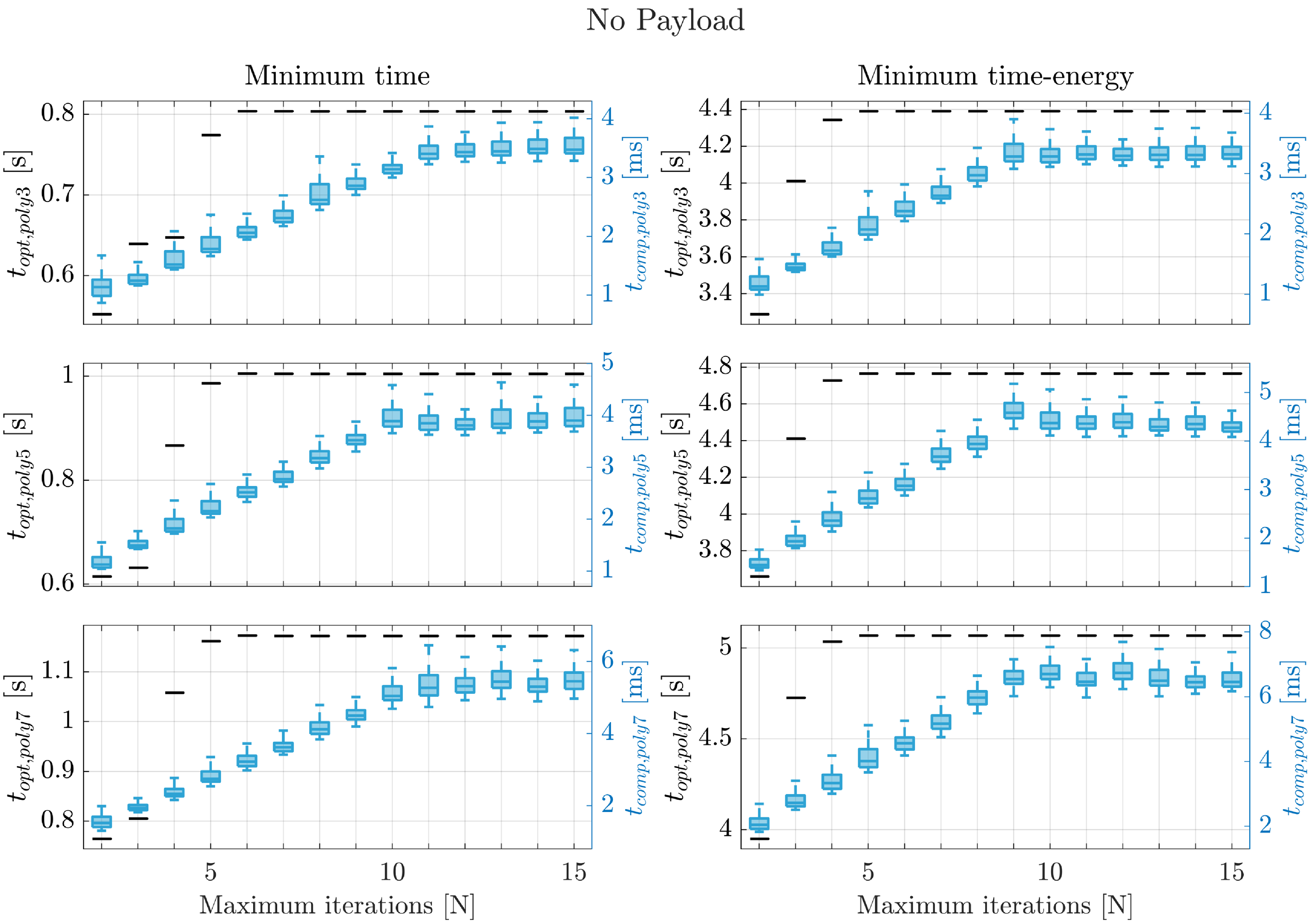
Box plot representation of the optimal times obtained and the computational times required for calculating the optimal solution as a function of the maximum number of iterations, for the case without payload, the two approaches, and the three motion laws considered, and for a traveled distance equal to
 $0.6\,{\rm m}$
(each test is repeated 100 times for statistical purposes).

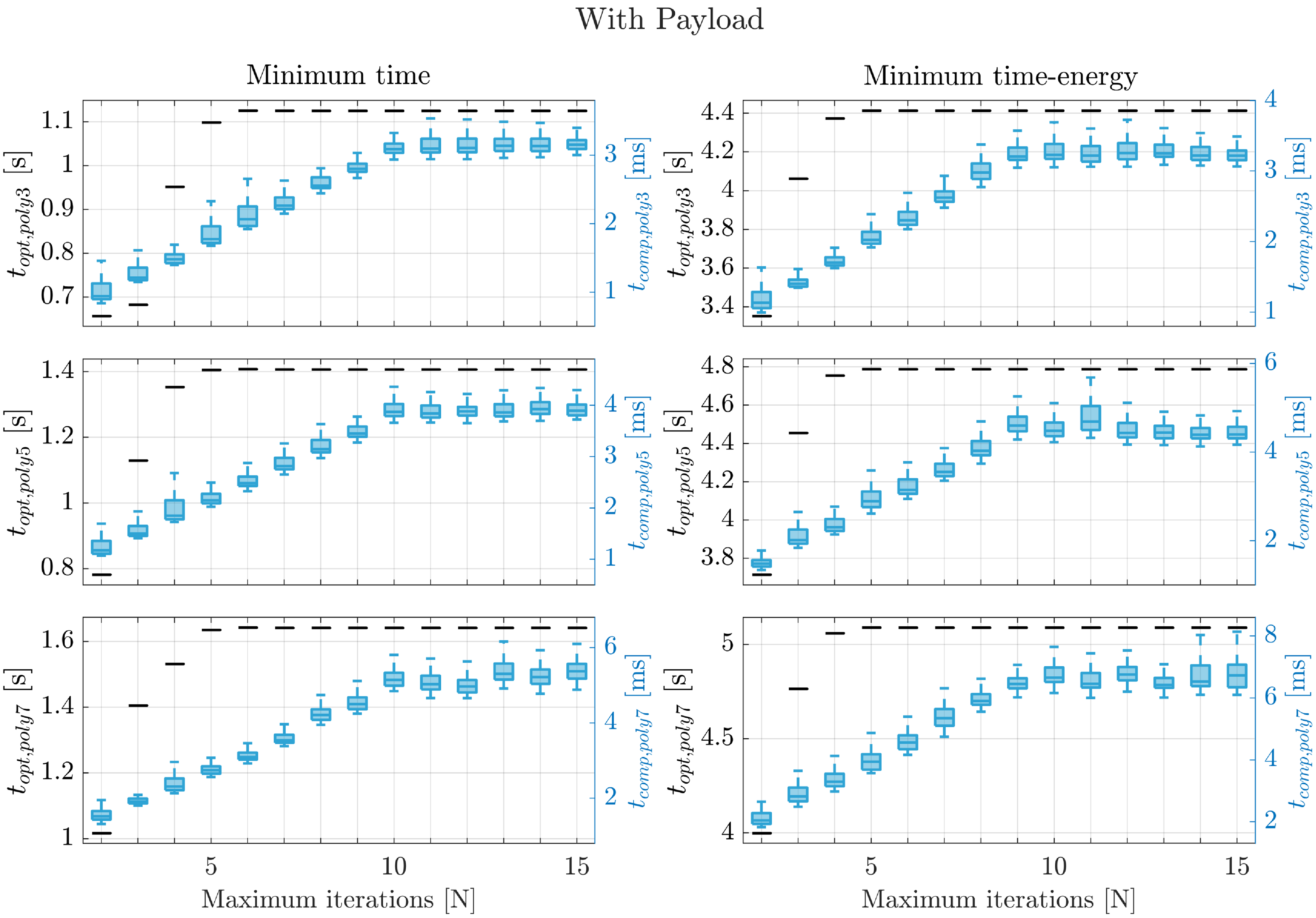
Figures 10 and 11 report the optimal execution time (black) and the box plot representation of the computational times (light blue) required for the optimization process as function of the maximum number of iterations. Figure 10 displays the data related to both considered approaches, the three motion laws, and the case without payload, whereas Figure 11 shows the same graphs for the case with payload. From the figures, it can be seen that, for both cases and both approaches, the solution found by the optimization within the maximum number of iterations converges to the optimal value of the execution time after just five or six iterations. For instance, in the minimum-time optimization using a poly3 motion law in the case without payload, the optimal value is approximately equal to
 $0.8\,{\rm s}$
, and 6 iterations are sufficient to find this solution. In the minimum-time optimization, values lower than the optimum represent a violation of the constraints. On the other hand, in the minimum-time-energy case, values lower than the optimum do not guarantee the best energy performance of the system. Furthermore, from Figures 10 and 11 it can be seen that the computational times increase with the polynomial degree for both cases and approaches, from about
 $3\,{\rm ms}$
for the poly3 trajectory, to about
 $4\,{\rm ms}$
for the poly5 motion law, to about
 $6\,{\rm ms}$
for the poly7 trajectory. Therefore, the computational times needed to obtain the optimal solution testify that the proposed approach is feasible for online trajectory optimization. Generally, for the same motion law, the minimum-time-energy approach requires slightly higher computational time with respect to the minimum-time one, since also the total mechanical energy of the system has to be computed (Eq. (2)).
Box plot representation of the optimal times obtained and the computational times required for calculating the optimal solution as a function of the maximum number of iterations, for the case with payload, the two approaches, and the three motion laws considered, and for a traveled distance equal to
 $0.6\,{\rm m}$
(each test is repeated 100 times for statistical purposes).

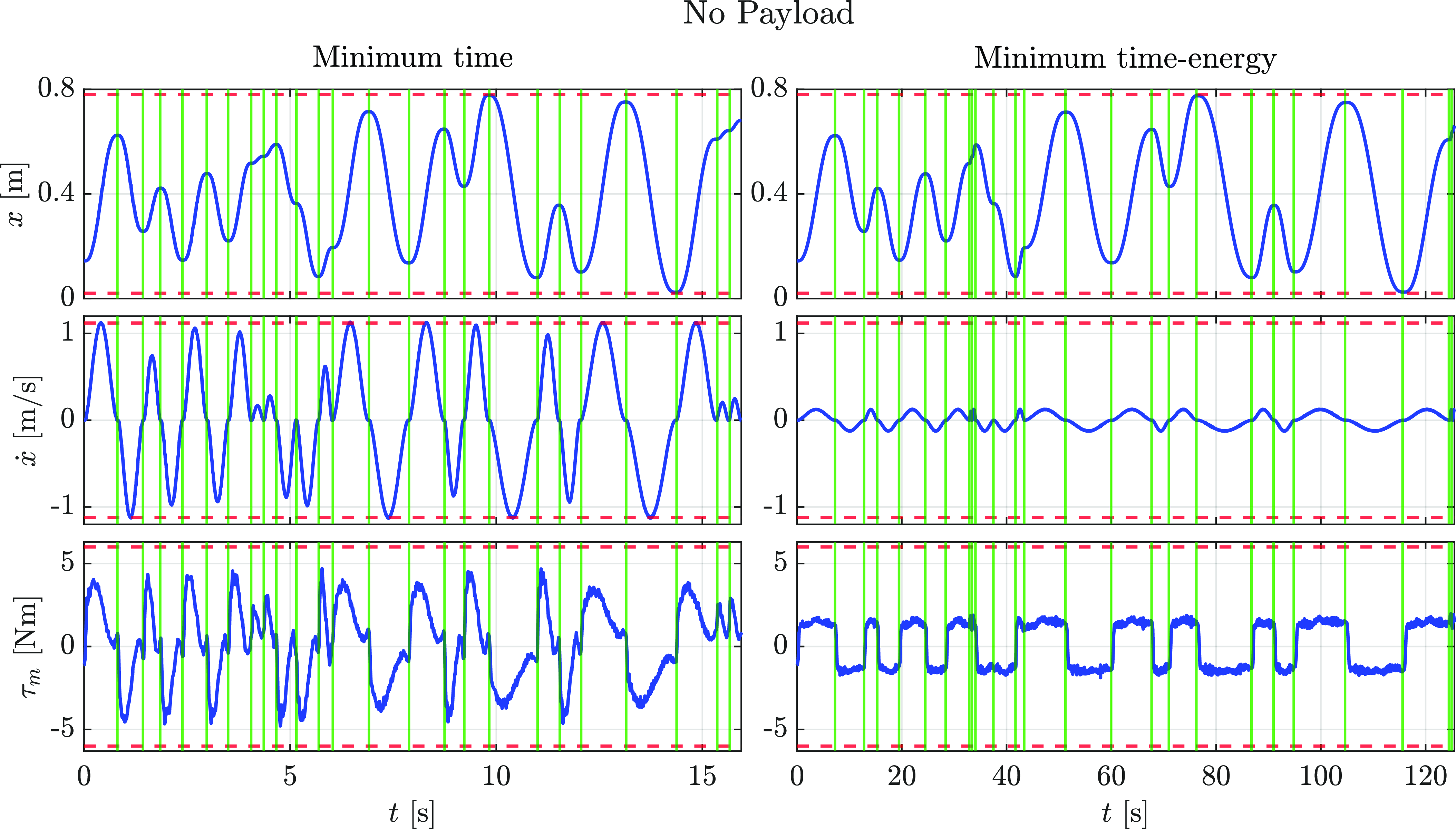
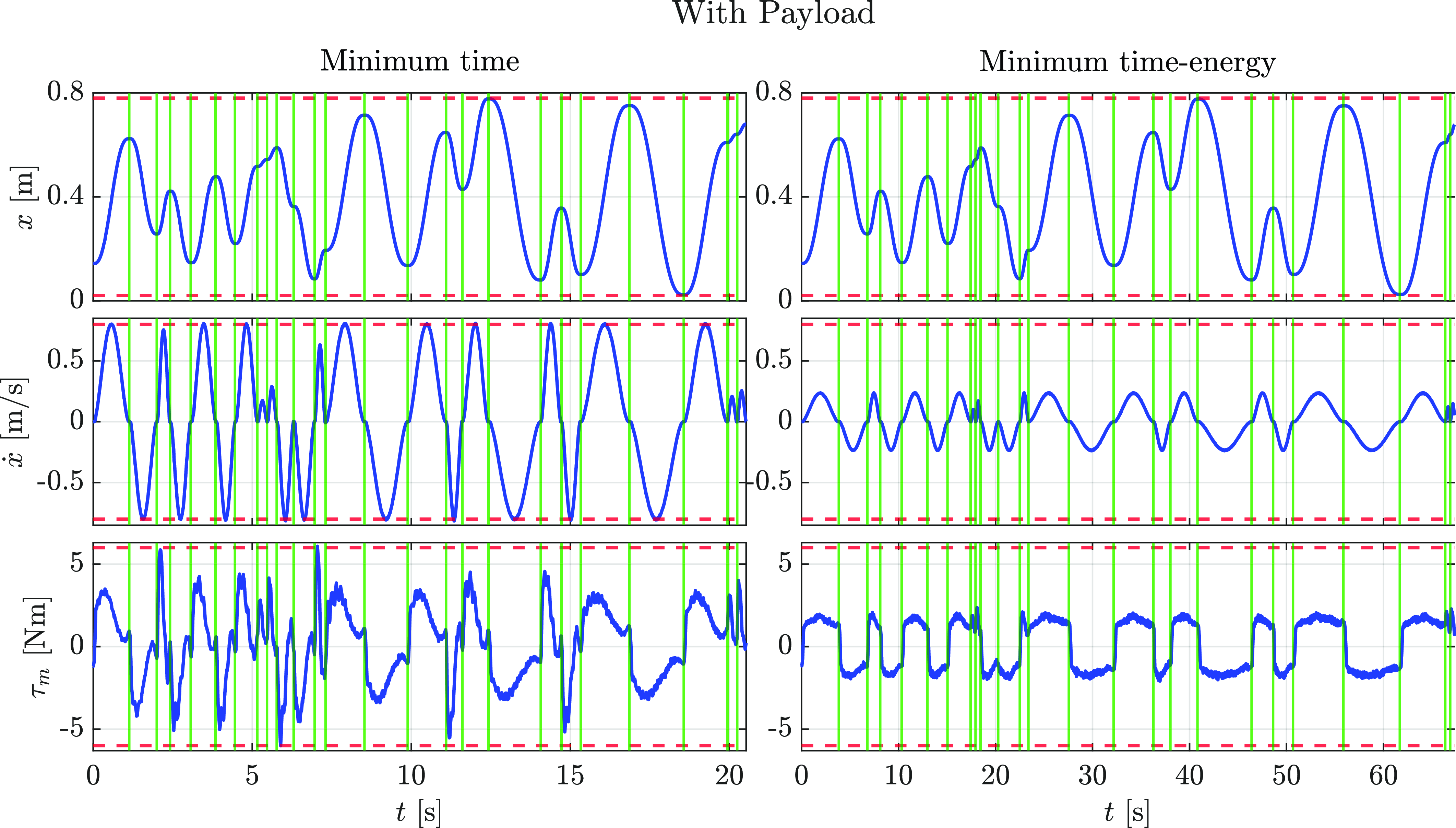
Joint position, joint velocity, and motor torque during the motions between 25 random waypoints, for both approaches, the case without payload, and the poly5 motion law.

The joint position, velocity, and motor torque over time through 25 exemplary waypoints for both approaches, the case of poly5 trajectories, and the case without payload are shown in Figure 12, whereas the same graphs for the case with payload are reported in Figure 13. The green vertical solid lines indicate the target waypoints, while the red horizontal dashed lines represent the joint limits. With reference to the results shown in Figures 10 and 11, the maximum number of iterations of the optimization is set equal to
 $12$
. From Figures 12 and 13 it can be seen that, for the minimum-time approach, the joint velocity and the motor torque peaks are close to the limits for both cases. This result evidences the capability of the proposed approach in finding the minimum execution time while meeting the kinematics and dynamics limits of the system. On the other hand, Figures 12 and 13 show that, considering the minimum-time-energy approach, for both cases the joint velocity and the motor torque are considerably lower with respect to the ones of the minimum-time approach, although the weight of the consumed energy in relation to the execution time is small. This is probably due to the high friction force of the linear axis, which leads to a considerable reduction of the cart velocity in order to decrease the motor torque needed and consequently the consumed energy.
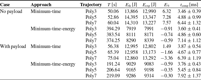
Experimental results: total execution time (
 $T = \sum _{i=1}^{99} \Delta t_i$
) of the trajectories between the 100 waypoints, mechanical energy spent during all trajectories computed with the dynamic model (
 $E_{{\rm th}}$
) and retrieved from the experimental data (
 $E_{{\rm exp}}$
), energy computation percentage error (
 $E_{\%} = [(E_{{\rm th}}-E_{{\rm exp}})/E_{{\rm th}}]\times 100$
), and optimization times (
 $t_{{\rm comp}}$
, mean
 $\pm$
standard deviation).

Joint position, joint velocity, and motor torque during the motions between 25 random waypoints, for both approaches, the case with payload, and the poly5 trajectories.

Finally, Table V illustrates the main experimental results of the proposed online optimization approach in terms of total execution time
 $T$
of all the point-to-point motions, theoretical and experimental mechanical energy consumption (
 $E_{{\rm th}}$
and
 $E_{{\rm exp}}$
, respectively) during all the trajectories between the 100 waypoints, and energy computation percentage error
 $E_\%$
. Considering the minimum-time approach, for both cases a smaller total execution time and a greater energy saving are achieved with the poly3 motion law with respect to the poly5 and poly7 ones. Instead, for the minimum-time-energy approach, the lower energy consumption is always obtained with the poly3 trajectory for both cases, but the lowest total execution time is obtained with poly7 motion law for the case without payload, whereas for the case with payload it is obtained with the poly3 trajectory. Furthermore, in Table V the computational times required for computing the optimal solutions are reported as mean
 $\pm$
standard deviation. As evidenced also from Figures 10 and 11, the computational times increase with the polynomial degree for both cases and approaches, and they are generally comprised between 3 and
 $8\,{\rm ms}$
.
The results presented in this paper show that the proposed optimization approach allows the system to plan and optimize online point-to-point trajectories based on a verified dynamic model. Furthermore, the proposed method is general and can be easily extended to other laws of motion and more complex robotic systems.
6. Conclusions
In this paper, an approach for the online optimization of minimum-time and minimum-energy point-to-point trajectories for a belt-driven robotic system has been presented. The optimization process leverages a verified dynamic model of the robotic system. In particular, an accurate identification of the friction parameters has been performed, comparing different friction models and assessing which one is most suitable for the considered system. Point-to-point motions of the linear axis have been planned online and executed sequentially, avoiding idle times by computing the optimal execution time for one trajectory during the execution of the previous one. In order to select the most suitable algorithm for the considered online optimization process, a comparison of the performance of three different open-source optimization tools in terms of computational times has been performed. Polynomial motion laws of degree
 $d$
equal to 3, 5, and 7 have been considered for the point-to-point motions. Furthermore, to assess the performance of the proposed online optimization approach under different dynamic conditions of the system, two cases have been considered, one without payload on the cart of the linear axis, and the other with a payload equal to
 $17.8\,{\rm kg}$
placed on the cart. The results of extensive experiments on the robotic linear axis have demonstrated the feasibility of the proposed approach for the online optimization of point-to-point motions, exhibiting computational times lower than
 $8\,{\rm ms}$
. Furthermore, the experimental results have shown the energy-saving capabilities of the proposed approach, as well as the flexibility of the online trajectory optimization in different scenarios, while meeting the kinematics and dynamics limits of the system.
In future work, we plan to adopt the robotic linear axis as a redundant prismatic joint for an industrial manipulator for energy efficiency applications in more challenging scenarios. Furthermore, we plan to adopt the approach presented in this work to enhance the flexibility and the operational efficiency of industrial robotic systems, paving the way for more sustainable and optimized automation solutions.
Supplementary material
The supplementary material for this article can be found at https://doi.org/10.1017/S0263574725001456.
Author contributions
All authors contributed to the study’s conception and design. Material preparation, data collection, and analysis were performed by Giuliano Fabris and Lorenzo Scalera. The first draft of the manuscript was written by Giuliano Fabris and Lorenzo Scalera, and all authors commented on previous versions of the manuscript. All authors read and approved the final manuscript.
Financial support
This work was developed within the Laboratory for Big Data, IoT, and Cyber Security funded by the Friuli Venezia Giulia region (Italy), and the Laboratory for Artificial Intelligence for Human-Robot Collaboration (AI4HRC) funded by Fondazione Friuli (Italy). This study was carried out within the Interconnected Nord-Est Innovation Ecosystem and received funding from the European Union Next-GenerationEU (Piano Nazionale di Ripresa e Resilienza, Missione 4, Componente 2, Investimento 1.5, D.D. 1058 23/06/2022, ECS00000043). This manuscript reflects only the authors’ views and opinions, neither the European Union nor the European Commission can be considered responsible for them.
Competing interests
The authors declare no conflicts of interest exist.
Ethical approval
Not applicable.