Nomenclature
Input parameters of compressor
- d
particle diameter (
 $\unicode{x03BC}$
m)
- m air
air mass flowrate (g/s)
- m sand
sand mass flowrate (g/s)
- p
compressor inlet pressure (Pa)
- rpm
compressor rotor revolutions per minute
- T
air or sand inlet temperature (K)

Output parameters from simulation
- LAC
particle accretion rate [g/(mm2 hr)]
- LER
erosion rate [g/(mm2 hr)]
- M
compressor flow Mach number
- p
compressor flow pressure (Pa)
- U
compressor flow or particle velocity (m/s)
Other symbols
- A
area (m2 or mm2)
- COR
coefficient of restitution
- k
turbulent kinetic energy (m2/s2)
-
$\Delta$
m
mass of sand particles impinging on target (g)
-
$\dot m$
mass of sand particles impinging the target per unit time (g/hr)
- R
radial coordinate (m)
- S
particle shape factor
- v n
particle normal velocity (m/s)
- v t
particle tangential velocity (m/s)
-
$\Delta$
W
sand erosion rate or ratio of target mass loss vs mass of sand particles impinging on target (g/g)
- X
coordinate in the cross-section (m)
- Y
coordinate in the cross-section (m)
- y
distance to the wall boundary (m)
- y +
non-dimensional distance of the first node away from a wall,
$\sqrt {{\tau _w}/{\rho _{_f}}} \,y\,/\,\upsilon $
- Z
coordinate in the longitudinal direction (m)
- α
impact angle defined as the acute angle between the particle velocity vector and plane tangent to the metal wall (degree)
-
$\rho$
density (kg/m3)
-
$\varepsilon$
energy to remove a unit mass from target material through deformation [g (m/s)2]
-
$\nu$
kinematic viscosity (m2/s)
-
$\tau_{w}$
w
wall shear stress (Pa)
-
$\varphi$
energy to remove a unit mass from target material through cutting [g (m/s)2]
-
$\omega$
turbulence specific dissipation rate (1/s)


1.0 Introduction
Sand erosion has long been recognised as a component degradation factor of air-breathing engines. Due to the higher hardness of the sand compared to steel or titanium compressor blades, as well as the high velocities at the engine inlet, ingestion of sand or other particles can cause significant component erosion, which affects the performance of the propulsion system and increases the cost of ownership, particularly for helicopters.
Sand erosion damage is dependent on many factors such as the blade geometry, operating condition, material/sand properties and engine flow field. Both experimental and numerical studies have been carried out to determine the features and intensity of compressor and turbine blade erosion. Grant & Tabakoff [Reference Grant and Tabakoff1] and Balan & Tabakoff [Reference Balan and Tabakoff2] performed experimental erosion studies on a single-stage axial compressor, made of 6,061 aluminium alloy. The experimental results revealed blunted leading edges, sharpened trailing edges, reduced blade chords and increased roughness of blade surfaces. Sugano et al. [Reference Sugano, Yamaguchi and Taguchi3] reported similar findings regarding the changes produced by erosion in axial-induced draft fans of coal-fired boilers. They also found that blade-chord reduction and material removal from the pressure surface increased with particle size. Richardson et al. [Reference Richardson, Sallee and Smakula4] carried out a diagnostic study on the JT9D high-pressure compressor and found that in general the changes correlated well with engine cycles, not with hours of engine service. Rotor-blade erosion was observed mainly in the outer 50% of the span, where significant reductions in the blade chord and thickness, and changes in the leading- and trailing-edge geometries were observed. Hamed et al. [Reference Hamed, Tabakoff and Wenglarz5] thoroughly reviewed erosion research in turbomachines and the associated degradation in engine performance caused by environment particle ingestion and confirmed the above findings.
Recently, a compressor blade erosion test rig was designed, constructed and commissioned at the Royal Military College of Canada (RMC) [Leithead, 2013; Massouh, 2012]. Erosion tests for bare and coated 17-4PH steel blades were carried out, and the blades were impacted by garnet sand for five hours. The experimental results provide useful information for understanding the blade erosion phenomenon and coating effectiveness and for validating erosion models.
To develop a sand erosion model, erosion coupon tests were carried out on 17-4PH steel blades at particle impact angles from 30o to 90o and velocities of 84 and 150m/s, respectively. In the testing, Al2O3 powder with an average size of 105
 $\unicode{x03BC}$
m was used as erosion media. The 17-4PH steel exhibited both cutting and deformation wear damage in comparable amounts, with erosion rates in the range of 800–1,300
 $\unicode{x03BC}$
g/g above an impact angle of 30o. Following the work from Bitter [Reference Bitter6] and Neilson & Gilchrist [Reference Neilson and Gilchrist7], Wu & Yang [Reference Wu and Yang8] derived a sand erosion model for 17-4PH steel.
In this paper, the above-developed erosion model for the 17-4PH steel is implemented into a CFD software solver and validated against the results of the compressor rig tests performed by RMC. In the following sections, the RMC compressor erosion rig test, the CFD simulation domain and mesh, the numerical methods and results are presented and discussed. Finally, a few key findings are highlighted.
2.0 RMC Compressor erosion rig and high-fidelity cfd model
2.1. RMC compressor erosion rig
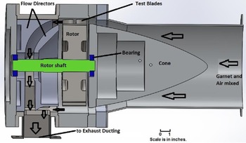
A sketch of the RMC compressor erosion rig is shown in Fig. 1. The rig was designed to rotate 16 blade assemblies at speeds up to 12,000rpm. The blade assemblies were inserted into a dynamically balanced 20.32cm diameter AISI 4,340 steel rotor that was driven by an aircraft gas turbine compressor gearbox and a 20 HP electric motor. The erosive media, garnet, was injected via a sand hopper into the rig, and to improve air/garnet mixing, a venturi mixer with a throat diameter of 89.2 mm was inserted in the housing pipe. A centrifugal blower supplied the air flow to the rig. Rig operating conditions were monitored from an operator station. The parameters monitored included rotor vibrations, rotor rpm, air flowrate, sand flow supply, etc. A full description can be found in Refs (Reference Leithead9) and (Reference Massouh10).
Schematic of the RMC compressor erosion test rig [Reference Bitter6].

Figure 2 is a cross-section view of the RMC compressor erosion rig test section, for clarity not all blade assemblies are included. The mixture of air and garnet flows over the central cone and enters a 12.7 mm annulus flow passage. The cone length is 0.305 m [Reference Massouh10, Reference Robinson and Delano11]. Immediately downstream of the cone, the annulus passage becomes straight with a length of 8.1 mm to keep the flow perpendicular to the blade leading edge. Further downstream, there is a 6.6 mm gap between the cone section and rotor section, used to accommodate 16 balance adjustment screw-heads.
Cross-section-view of the RMC compressor erosion rig test section [Reference Sugano, Yamaguchi and Taguchi3].

2.2. Compressor blade and assembly
The test blade profile is named as V 103, which is a modified version of a NACA 6,505 aerofoil. For the modified aerofoil, the leading-edge radius is 0.19 mm, and the trailing edge radius is 0.15 mm. The modified blade profile normalised by the chord length is shown in Fig. 3. The test blade chord is 26.67 mm, and the span is equal to 12.7 mm minus the averaged tip clearance of 0.64 mm, i.e. 12.06 mm. The blade is made of 17-4PH steel, commonly used in turbine engines. More details are available in Ref. (Reference Bitter6).
The V103 blade profile.

A top view of one blade-dovetail assembly is given in Fig. 4, where the test blade and dummy blade arrangement relative to the dovetail block is illustrated. To prevent a requirement for a larger electric motor, a two-blade arrangement was designed. The upstream blade acted as the compressor test paper, and the downstream one simply flipped its pressure/suction sides and redirected the flow. In this way, the requirement for an excessively high-power input was avoided. The dimensions of the dovetails are: 25.4 mm wide and 58.4 mm long. The stagger angle is 27.7 degree, and the distance between two blades was 10.4 mm. Reference (Reference Bitter6) contains additional details.
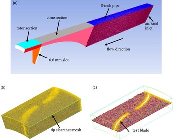
Computational domain and mesh, (a) the whole domain and mesh, (b) the rotor section mesh, and (c) the mesh across rotor middle section.

2.3. Computational domain and mesh
The computational domain and mesh are illustrated in Fig. 4, which is a 22.5o or 1/16 sector of the flow field. The domain includes an 8-inch straight pipe segment, cone section, rotor section and 6.6 mm slot. It consists of one blade assembly flow passage, begins downstream of the venturi diverging section and is extended 20 mm downstream of the rotor section.
As observed in Fig. 4, fine grids were laid at the blade surfaces, in the downstream region of the cone section, as well as in the narrow tip clearance region. The tip clearance is only 0.64 mm, and six grids were generated in the vertical direction. The y+ value is in a range of 20–55 for the blade, blade tip, and casing wall. Effort was made to keep y+ values in the range of 30–150 for the remaining walls. A few meshes were created and preliminary runs were performed to improve the quality of numerical simulations. The solution mesh independence was checked, and the deviation between the 2.8 million and 6.9 million cell cases at the rotor middle cross-section was only 1.2% for the mean Mach number, and 0.69% for the maximum Mach number. Finally, a mesh of 4.3 million cells was used for all simulations.
3.0 Numerical methods
Two phase, compressible, turbulent flows in multiple reference frames were considered in the present work. A commercial software package, ANSYS CFD Premium, was used for all numerical simulations. To account for compressor blade erosion, the erosion model from Wu & Yang (Reference Wu and Yang8) was implemented into the software package. In the following sub-sections, the compressor input parameters, numerical approaches, implementation of the compressor erosion model, other physical models and solution methods are briefly described.
3.1. Inputs parameters of RMC compressor rig testing
The input parameters from the RMC compressor test rig are given in Table 1. The air and sand inlet mass flowrates are 1/16 of the total air and sand flowrates in testing.
Test rig operating conditions

To account for the pressure loss behind the rotor section, the pressure at the computational domain exit was adjusted to match the Mach number of 0.34 at the rotor inlet. The pressure at the domain air inlet was defined as atmospheric, and the tiny pressure loss from the blower to the air inlet was neglected. For the 6.6 mm slot in Fig. 4(a), the cone section side was assigned as a stationary wall, and the rotor side was defined as a moving wall. Moreover, the rotor shaft (d = 43 mm) wall was also a moving wall.
Note that the corresponding sand concentration in air is 2.51g/m3 of air based on the air and sand flowrates in Table 1. This value is somewhat higher than the field measured values of 2.16g/m3 as the maximum, and 1.16g/m3 as an average [Reference Cowherd12]. In this sense, the RMC testing could be considered as an accelerated erosion case.
As mentioned earlier, garnet was used as the erosion media to represent sand in the rig testing, and Table 2 shows the particle distribution by size and weight.
Particle distribution by size and weight for Barton UT220 garnet abrasive

The specific gravity of the garnet abrasive is 4,000kg/m3 and the Mohs hardness is 7.5–8.5 [13].
3.2. Simulations in multiple reference frames and Eulerian-Lagrangian approach
As the simulation concerns rotating machinery, the computational domain includes both stationary and moving components, i.e. the standing rig components and rotating rotor, respectively. A moving reference frame concept is introduced to render problems that are unsteady in the stationary frame steady with respect to the moving frame. The details of the steady Favre-averaged conservation equations in an inertial or stationary reference frame, and the flow velocity transformation between the stationary and moving frames can be readily found in Refs (Reference Ferziger and Peric14) and (15).
In the present study, two reference frames—one stationary and one moving—are employed, and the mixing-plane approach is used for interfacing between these two frames. The main advantage behind the mixing-plane approach is that each fluid zone can be solved as a steady-state problem. The flow data at the mixing plane interface are averaged in the circumferential direction at the cone section outlet and rotor inlet boundaries. By performing circumferential averages along 66 radial stations in the mixing plane, the “profiles” of flow variables can be defined and then used to update boundary conditions of the cone and rotor sections at the mixing plane. Despite the simplifications inherent in the mixing-plane approach, the resulting solutions can provide reasonable results of the time-averaged flow field [Reference Tallman, Haldeman, Dunn, Tolpadi and Bergholz16]. Considering the speed of the blade rotation, 10,860rpm, it is anticipated that the effect of the unsteadiness on the flow field would fade out.
The traditional Eulerian-Lagrangian approach is used to solve two-phase, turbulent, compressible flows in the two reference frames. For the present work, the volume fraction of garnet particles is negligibly small, 6.7E10−7, and thus the dilute discrete Lagrangian particle tracking method is an ideal approach without compromising the numerical solutions [Reference Stiesch17]. With this approach, the fluid phase is treated as a continuum by solving a set of governing equations, while the dispersed solid phase is solved by tracking many particles through the calculated flow domain. The exchanges of momentum, mass and energy between particles and fluid can be included if necessary.
The drag coefficients for both spherical and non-spherical particles are based on comprehensive experimental measurements [Reference Morsi and Alexander18, Reference Haider and Levenspiel19]. For sand particles, a shape factor of 0.516 is suggested [Reference Taslim, Khanicheh and Spring20, Reference Duffy21]. In the numerical simulations, for each group of particles in Table 2, the Rosin-Rammler size distribution was assumed, and there were 2,620 particle streams. As a result, there were a total of 18,340 particle injection streams.
3.3. Particle rebound characteristics
It is recognised that particle rebound characteristics at walls play an important role in particle trajectory calculations. Considerable research in this area was conducted by Wakeman and co-workers [Reference Taslim, Khanicheh and Spring20, Reference Wakeman and Tabakoff22, Reference Taslim and Spring23]. The experiments were carried out with 165µm silica particles impinging on 2025 AL, INCO 718 and Ti 6-4 target walls with the impinging angles 15o–90o and particle velocities 27–273m/s. They pointed out that particle rebound characteristics were generally influenced by impingement angle and not significantly affected by target material or temperature tested. The semi-empirical coefficients of restitution for tangential and normal velocities, CORt and CORn, before and after collision obtained from their measurements are used in the present work
 \begin{align}CO{R_t} = \frac{{{V_{t2}}}}{{{V_{t1}}}} = - 3.562 \times {10^{ - 6}}{\alpha ^3}+6.427 \times {10^{ - 4}}{\alpha ^2} - 2.897 \times {10^{ - 2}}\alpha +0.\;988\end{align}
 \begin{align}CO{R_n} = \frac{{{V_{n2}}}}{{{V_{n1}}}} = - 2.605 \times {10^{ - 6}}{\alpha ^3}+4.752 \times {10^{ - 4}}{\alpha ^2} - \;3.072 \times {10^{ - 2}}\alpha \;+0.\;993\end{align}
where vt and vn are particle tangential and normal velocity components, α is particle impact angle in degrees, and the subscripts 1 and 2 indicate particle parameters before and after collision, respectively. The variations of tangential and normal coefficients of restitution with the particle impact angle are illustrated in Fig. 5.
Variation of CORt and CORn with particle impact angle.

To model turbulent momentum transfer in the flow field, the SST k-
 $\omega$
model (the shear-stress transport-model) was applied. This model has illustrated major improvements in the prediction of adverse pressure gradients and separation flows over the standard k-
 $\omega$
and k-
 $\varepsilon$
models and has been widely used in turbine machinery flows [Reference Menter24]. The turbulence scalar transfers were calculated based on the modeled momentum transfer, where the turbulence Prandtl and Schmidt numbers of 0.75 were used. At the wall boundaries, the enhanced wall treatments were used for both turbulence kinetic energy and specific dissipation rate, where the viscous sublayer and the logarithmic layer formulations were smoothly blended [ANSYS Canada Ltd., 2018].
3.4. Erosion model implementation and check
As mentioned, Wu & Yang [Reference Wu and Yang8] carried out erosion experimental studies on 17-4PH steel coupons and developed an erosion model for 17-4PH compressor blades. From these tests, the erosion rate (or ratio of the target mass loss to the mass of sand particles impinging on the target) for the 17-4PH steel can be evaluated by the following equations in unit of g/g:
 \begin{align}\Delta {W_a} = \frac{1}{2}\Delta {m_a}{U^2}co{s^2}{\rm{\alpha }}\sin \left( {n\alpha } \right)/\varphi {\rm{\;}} + \frac{1}{2}\Delta {m_a}{\left( {Usin\alpha - K} \right)^2}/\varepsilon \quad \alpha \le {\alpha _0} = \pi /2n\end{align}
 \begin{align}\Delta {W_b} = \frac{1}{2}\Delta {m_b}{U^2}co{s^2}{\rm{\alpha }}/\varphi {\rm{\;}} + {\rm{\;}}\frac{1}{2}\Delta {m_b}{\left( {Usin\alpha - K} \right)^2}/\varepsilon \quad \alpha \ge {\alpha _0} = \pi /2n\end{align}
where α is the impact angle, αo stands for the impact angle at which the horizontal velocity equals zero when the particle leaves the surface,
 $\Delta$
m
a and
 $\Delta$
m
b are the accumulated mass of particles impinging on the target material for the impact angle less and larger than αo, respectively, U is the particle velocity magnitude, n and K are constants related to the target material,
 $\varphi$
and
 $\varepsilon$
represent the energies required to remove a unit mass from the target material though the cutting and deformation actions, respectively. The model parameters are given in Table 3.
Erosion model parameters

Considering local area and erosion duration, the local erosion rate can be defined as
 \begin{align}{\rm{LER}} = \Delta\ \textrm{W}{\rm{/}}\textrm{A}^{*}\dot m = (\Delta {\textrm{W}_a} + \Delta {\textrm{W}_b})/\textrm{A}^{*}\dot m\end{align}
where A (mm2) is the local surface area,
 $\dot m$
(g/hr) is the mass of sand particles impinging on the local area per unit time, and the unit LER is [g/(mm2 hr)], which stands for the material mass loss per mm2 per hour at the sand injection rate in the erosion testing, (0.1475g/s, the above sub-section 3.1).
Note that the erosion model input parameters include the four variables in Table 3, as well as the particle impact angle, mass and velocity magnitude impinging on the metal wall. The last three parameters are obtained as particles travel through the flow field and impinge on the metal wall. The output parameters are local and total erosion rate (LER) or local and total mass loss at the defined test rig operating conditions.
A user-defined function is written to compile and link the above erosion model to the ANSYS CFD Premium flow solver. To ensure the erosion model was properly implemented, a few simple flows consisted of two pipes connected by a step with varying slope, as shown in Fig. 6, were used. For each numerical test case, the flow velocity was generated according to the erosion model test velocity, and one particle with a mass of one gram was released from a selected position in the flow. Trial and error were performed to match the experimental test conditions in terms of impact angle and velocity magnitude. All the above seven model parameters and metal mass loss due to the particle impingement were printed out on the screen, checked and compared with the experimental data.
A simple two-pipe flow to check erosion model implementation, (a) the flow field and a particle trajectory, and (b) the particle impact angle α.

In Fig. 7, the erosion rates obtained from simulations with a particle flowrate of 1.0g/s at several impact angles and velocities are compared with the model curves from Equations (3) and (4). The computed results match the model curves, which indicates that the erosion model is correctly implemented into the flow solver.
Comparison between the computed and modeled erosion rates.

A pressure-velocity coupled solver with a second-order accurate scheme was used to resolve the flow-field. As the flow reaches steady or quasi-steady, the scaled residuals of flow variables were less than 6 × 10⁻⁷ for velocity components and energy, and about 3 × 10⁻⁵ for turbulent variables. The monitored flow parameters remained unchanged at least for the first four significant digits. A LINUX cluster, 12-cores and 64 GB RAM, was used for all simulations.
4.0 Results and discussion
4.1. Flow-Field in the rotor vicinity
The distributions of velocity magnitude, Mach number and static pressure at the symmetric plane in the vicinity of the rotor section are displayed in Fig. 8. The flow velocity and Mach number increase gradually towards the rotor section and reach maxima in the rotor section due to the flow cross-section area gradual decrease. Consistent with the above, the static pressure gradually decreases towards the rotor section and reaches a minimum value in the rotor section.
Contours of velocity magnitude, Mach number and static pressure at the symmetric plane.

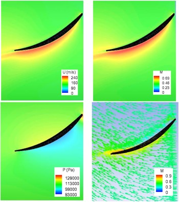
The velocity, Mach number, static pressure and velocity vector distributions across the mid-span of the test blade are illustrated in Fig. 9, viewed from top of the rotor section. The rotor rotates in the clockwise direction, looking upstream (or the blades are moving left to right). As expected, the velocity and Mach number contours are similar. The velocity and Mach number are low on the pressure side, gradually increase towards the trailing edge and are high on the suction side, from ∼1/6 downstream of the leading edge. The flow stagnation point is clearly indicated in the pressure plot, i.e. the highest pressure occurs at the blade leading edge. The pressure is low on most of the suction side due to flow acceleration, while along the pressure side the pressure gradually increases before decreasing near the trailing edge. In the vector plot, the velocity vectors stand for the combined in-coming axial velocity and rotor rotating velocity, where the vector magnitude is coloured by Mach number.
Contours of velocity magnitude, Mach number and static pressure, as well as absolute vectors across the mid-span of the test blade.

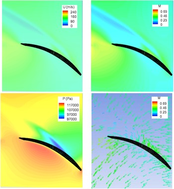
Figure 10 presents the distributions of velocity magnitude, Mach number and static pressure, and a velocity vector plot across the mid-tip-clearance over the test blade. To show the test blade tip location, these plots are rotated 180 degrees over the Z axis and viewed outwards from the rotor centre (put another way, the blades are moving right to left). The flow at this cross-section is complicated. It is affected by the stationary incoming flow from the cone, the blade rotating flow, and the stationary casing wall, as well as the associated interactions. As shown in the vector plot, the flow over the blade tip moves from the pressure side to the suction side, against the main flow direction, and the tip vortex is generated downstream of the suction side. Because of the tip leakage, a relative high velocity and Mach number region occurs at the front portion of the suction side, while the velocity and Mach number are relatively low over the pressure side. The pressure patterns are consistent with the velocity and Mach number distributions.
Contours of velocity magnitude, Mach number and static pressure, as well as absolute vectors across the mid-tip-clearance over the test blade.

The distributions of velocity magnitude, Mach number and static pressure at the mid-cross-section of the 6.6 mm slot are illustrated in Fig. 11, where the 12.7 mm annulus inlet section is indicated by black lines. This flow is influenced by the incoming annulus flow from the cone section, the rotor rotating flow, the stationary wall on the cone side and the moving walls on the rotor side and rotor shaft. In general, the slot flow is rotating around the rig longitudinal axis caused by the moving walls, and vortices occur just below the annulus channel generated by the incoming annulus flow. As seen in the three plots, the effect of the slot flow on the main annulus flow is negligible. The flow parameters gradually increase from the bottom to top, except that in the pressure plot there is a low-pressure region below the annulus flow. This low-pressure region is where a small vortex occurs across the 6.6 mm slot with its axis perpendicular to the flow longitudinal plane, and it is generated by the in-coming annulus flow. Detailed analysis is beyond the scope of the present work.
Contours of velocity magnitude, Mach number and static pressure at the mid-cross-section of the slot.

4.2. Particle trajectories
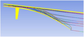
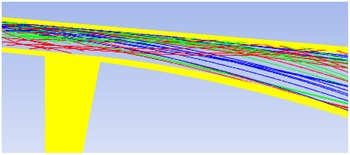
Typical particle trajectories around the test blade are shown in Fig. 12 for particle diameters of 115, 68.5 and 22.5
 $\unicode{x03BC}$
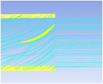
m, represented by red, green, and blue lines, respectively. Figure 13 gives representative flow path-lines passing through the test blade, where the flow path-lines follow the blade profile in general. In these two plots, the test blade and rotor periodic surfaces are shown in yellow colour. The three path-lines across the blade indicate that the air flows over the blade tip through the tip clearance. The airflow at the rotor section entry experiences a sudden velocity increment, i.e. gaining a large rotating circumferential velocity; however, the particles cannot fully follow the airflow change due to their inertia. As seen in Fig. 12, for the particles starting at nearly the same upstream location, the larger the particle size, the further upstream the impingement point.
Typical particle trajectories around the test blade for d = 115, 68.5 and 22.5
 $\unicode{x03BC}$
m, coloured in red, green, and blue lines, respectively.

Typical flow path-lines around the test blade.

Figure 14 shows numerous particle trajectories traversing through the cone and rotor sections for d = 115, 68.5 and 22.5
 $\unicode{x03BC}$
m, respectively, where all walls are shown in yellow. Almost all particles impinge on the test rig wall, bounce back, and move forward in the flow passage. Their trajectories are different, depending on particle size, impact angle and injection location at the air/sand inlet. Figure 15 displays some of sand particle trajectories passing through the rotor inlet cross-section for d = 115, 68.5 and 22.5
 $\unicode{x03BC}$
m. For this cone configuration, more particles enter the rotor section through the upper portion of the cross-section, and less particles enter the rotor section through the lower portion of the cross-section. This phenomenon is consistent with the observation by Richardson et al. [Reference Richardson, Sallee and Smakula4] on the JT9D high-pressure compressor, as mentioned earlier.
Typical particle trajectories through the cone and rotor sections for d = 115, 68.5 and 22.5
 $\unicode{x03BC}$
m, coloured in red, green, and blue lines.

Particle trajectories through the rotor inlet cross-section, d = 115, 68.5 and 22.5
 $\unicode{x03BC}$
m, coloured in red, green, and blue.

4.3. Sand particle accretion rate, velocity magnitude, and impact angle
The particle accretion rate is defined as the accumulated mass of sand particles impinging on the local metal surface per unit time, i.e.
 \begin{align}{\rm{LAC}} = \dot m\;{\rm{/}}\textrm{A}\end{align}
As in Equation (5), A is the local surface area,
 $\dot m$
is the mass of sand particles impinging on the local area per unit time, and the unit of LAC is [g/(mm2 hr)], which gives the accumulated mass of sand particles per mm2 per hour at the sand injection rate, 0.148g/s.
The distributions of sand particle local accretion rates at the pressure and suction sides of the test blade are displayed in Figs 16 and 17 after one hour of exposure to the sand impingement, where the rotor bottom wall is outlined by black lines. The maximum accretion rate reaches ∼9.0 g/(mm2 hr), and the average value over the test blade is 0.46 (g/mm2 hr). The total mass of particle impacting on the test blade in one hour is 0.318kg, and the total sand delivered in one hour to the 22.5o rotor sector is 0.531kg. That is, more than half of the sand particles delivered strike the test blade.
Sand accretion rate distribution on the pressure side.

Sand accretion rate distribution on the suction side.

Three important features are observed in Figs 16 and 17, and it should be noted that the scales in the two figures differ by orders of magnitude. First, most of the sand particles impinge on the pressure side, and only a limited number of particles impact on the suction side near the leading edge. This is consistent with the observations by many researchers such as Balan & Tabakoff [Reference Balan and Tabakoff2], Sugano et al. [Reference Sugano, Yamaguchi and Taguchi3] and Hamed et al. [Reference Hamed, Tabakoff and Wenglarz5]. Second, as shown in Fig. 16, severe erosion occurs mainly at the outer ∼50% of the span, which agrees with the finding from Richardson et al. [Reference Richardson, Sallee and Smakula4]. It is also consistent with the particle trajectories observed in Fig. 15. Third, more particles impact the downstream half of the blade on the pressure side, and this can be explained by the observation in Fig. 12. Due to the inertia, particles impact the blade surface because they cannot follow exactly the airflow path-lines.
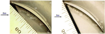
The above observations are consistent with those in the RMC compressor rig testing, although some photos in the report [Reference Leithead9] are not sufficiently clear for comparison. Figure 18 shows the rear pressure surface of the test blade before and after five hours of erosion. The rear portion of the pressure side is heavily polished by particles, particularly for the upper portion. This is consistent with the simulation results in Fig. 16.
Test blade rear pressure surface: (a) before erosion, (b) after five hours of erosion (scale in 1 mm per increment and 8x magnification).

The blade cross-section profiles before and after five hours of erosion are illustrated in Fig. 19. It is apparent that the blade trailing edge is sharpened due to erosion. This is also consistent with the observation in Fig. 16, where more particles impacted the trailing-edge region. The comparisons between the experimental observations in Figs 18 and 19 and the numerical results in Fig. 16 indicate that the developed sand erosion model is adequate for engine components made of 17-4PH steel.
Sharpened trailing edge of the test blade: (a) before erosion, (b) after five hours of erosion (scale in 1 mm per increment and 6.3x magnification).

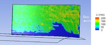
In addition to the accretion rate, other parameters related to particle erosion are obtained in the simulation, which provides additional information to aid in understanding of the erosion phenomena. The velocity magnitude distributions of sand particles impacting on the pressure and suction sides are presented in Figs 20 and 21, respectively, where the blue region means no particle impingement and the white arrow indicates the incoming flow direction. The maximum velocity magnitude reaches ∼190m/s, and the maximum value at the suction side is higher than that at the pressure side due to flow acceleration at the suction side. The distribution features are the same as Figs 16 and 17, i.e. most of particles strike on the pressure side. Moreover, on the pressure side, the particle velocities are higher in the upstream region than those at the downstream portion. It is anticipated that the flow velocity near the pressure side gradually decreases as shown in Fig. 9.
Velocity magnitudes of particles impacting the blade pressure side.

Velocity magnitudes of particles impacting the blade suction side.

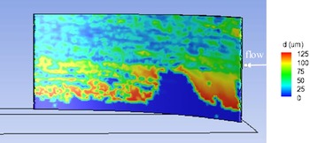
The diameter distributions of particles impacting the blade pressure and suction sides are displayed in Figs 22 and 23, respectively. The maximum particle diameter is 125
 $\unicode{x03BC}$
m as defined in the air/sand inlet, and the contour features are similar to the velocity contours in Figs 20 and 21. It is interesting to note that large particles more commonly strike the blade lower surfaces, instead of a uniform distribution. This can be readily explained by the variation of particle trajectories with their sizes, as shown in Figs 14 and 15. The particle trajectories are determined by the cone configuration, rotor section walls and particle properties.
Particle diameters impacting the blade pressure side.

Particle diameters impacting the blade suction side.

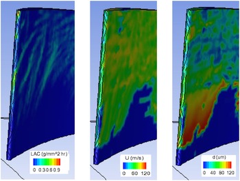
The contours of sand particle accretion rate, impinging velocity and diameter in the vicinity of the leading edge are given in Fig. 24. Sand particles heavily strike the leading edge from ∼1/3 of the span to the tip, and large particles hit the lower portion of the leading edge as seen in Figs 22 and 23. Figure 25 is a photo of the blade cross-section profile after five hours of testing. The round leading-edge tip at the pressure side becomes bowed and blunt, which is consistent with the simulation result. Rapid erosion at the leading edge from the middle span to the tip is also observed in a similar erosion testing with the same test rig [Reference Leithead, Allan, Zhao and Yang25].
Contours of sand particle accretion rate, impinging velocity and diameter near the leading edge.

Blade leading cross-section profile after 5 hours of testing (scale in 1 mm per increment and 40x magnification).

In summary, Figs 16–25 demonstrate that the numerical simulation results are consistent with the test results from the RMC compressor rig and the experimental findings from other researchers. The sand erosion blunts the leading edge, sharpens the trailing edge and increases pressure surface roughness. For the present rig geometry, in particular the cone geometry, few particles strike the blade root area, and more particles hit the upper area of the blade pressure side. Also, greater particle accretion occurs at the rear portion of the chord than the forward region.
4.4. Sand erosion rate
In the previous sub-section, the numerical results were qualitatively compared with the experimental results from the RMC and other researchers. In this sub-section, the sand erosion rate from the simulation is compared with those from other erosion models. Figures 26 and 27 display the contours of local sand erosion rate at the blade pressure and suction sides from the current simulations. As expected, severe sand erosion occurs on the pressure side, particularly at the rear upper region, and the erosion rate at the suction surface is negligible, except in the vicinity of the leading edge (note the scales differ by about two orders of magnitude). These support the features of particle accretion discussed in the previous sub-section. The maximum erosion rate reaches 6.3 (mg/mm2 hr), the average is 0.39 (mg/mm2 hr), and the blade mass loss is 0.273 (g/hr).
Sand local erosion rate on the blade pressure side.

Sand local erosion rate on the blade suction side.

In Table 4, the predicted sand erosion rate is quantitatively compared with three other sand erosion models. The first model is Finnie Erosion model [Reference Finnie26], and its model constants have been tuned to match the experiment data in Ref. (Reference Oka and Yoshida27), where 326
 $\unicode{x03BC}$
m sand particles impinged on a carbon steel wall at a speed of 104m/s. The second is McLaury model for predicting the erosion rate of sand particles on carbon steel in water [Reference McLaury28]. The third is Oka erosion model with the constants calibrated for sand erosion on carbon steel [Reference Oka and Yoshida27]. The maximum erosion rate, average erosion rate and total blade mass loss predicted by the four sand erosion models are listed in Table 4. Recall that these numbers are obtained based on a sand flowrate of 0.148g/s or 0.531kg/hr passing through the 22.5o rotor sector. As shown in Table 4, the predicted values from the current model are lowest among these four models since the mechanical properties of 17-4PH steel are better than carbon steel. The predicted mass loss from the 17-4PH model is 13% lower than the average mass loss from the three carbon steel models, which indicates that 17-4PH steel has stronger resistance to sand erosion than carbon steel.
Sand local erosion rate and blade mass loss

5.0 Conclusions
Sand or other particles can cause significant degradation to propulsion system performance, and increase the cost of ownership, particularly for helicopters. Based on erosion tests on 17-4PH steel coupons, a sand erosion model has been developed. In this work, the developed erosion model has been validated against the results of the RMC compressor rig tests and other published results. A high-fidelity CFD model of the RMC test rig has been built; the two-phase, turbulent, compressible flow-field in multiple reference frames has been solved, and the developed erosion model has been implemented into the ANSYS CFD Premium software and checked step by step.
The simulation results are consistent with the test results from the RMC compressor rig and experimental findings from other researchers. Sand erosion blunts the leading edge, sharpens the trailing edge and increases pressure surface roughness. For the present rig geometry, particularly for the cone geometry, few sand particles strike the vicinity of the blade root, and most particles hit the large upper area on the blade pressure side. More particle accretion is found at the rear half of the chord than the forward region.
The comparisons between the experimental observations and numerical results as well as a quantitative comparison with three other sand erosion models indicate that the developed sand erosion model is adequate for erosion prediction of engine components made of 17-4PH steel. The predicted mass loss from the 17-4PH model is 13% lower than the averaged mass loss from the three carbon steel models, which indicates that 17-4PH steel has stronger resistance to sand erosion than carbon steel. Furthermore, the established methodologies can also be used to evaluate the effect of erosion-resistant coating and the erosion degradation of components under actual engine operating conditions.
Acknowledgments
The authors are grateful to the Department of National Defence and the National Research Council of Canada for funding and supporting this collaborative research project. Also, many thanks go to Dr. Steve Zan for the valuable comments and suggestions in the preparation of the manuscript.