1. INTRODUCTION
Real-Time Kinematic (RTK) positioning technology is based on high-precision carrier phase observation and can quickly provide Three-Dimensional (3D) coordinates in real-time, with an accuracy approaching the centimetre to millimetre level. The basic principle of RTK technology can be described as follows: in a certain area (several square kilometres), one receiver, called the base station, is set up at a point with known coordinates. Other receivers are then set up in the local area, called rover stations. By broadcasting accurate coordinates and raw observations from the base station to the rover stations, the rover stations can complete a Double-Differenced (DD) solution and ambiguity resolution to realise high-precision and real-time dynamic positioning (Rizos, Reference Rizos2007; Zhang et al., Reference Zhang, Teunissen and Odijk2011a).
Because of its characteristics of high precision, high efficiency and ease in achieving real-time performance, RTK has been widely used in many types of survey engineering. However, there are also two major problems in the application of RTK. The first is environmental influence. Signal transmission may be blocked by buildings, trees, etc. Also, the measuring time may be influenced by ionosphere activity characteristics, number of observed satellites and other signal constraints. Thus, initialisation may take a long time or may not be possible at all. The second problem is a distance limitation, as the basic principle of RTK is to eliminate errors related to a particular location. With an increase in operating range, the spatial correlation of errors decreases, and the positioning accuracy is gradually reduced. The initialisation time is longer, and the working distance of the RTK is effectively limited to only a few kilometres (Gao and Liu, Reference Gao and Liu2003; Zhang et al., 2010b; Wang et al., Reference Wang, Bei and Li2014).
Recently, various Continuously Operated Reference Station (CORS) networks and local augmentation using Global Navigation Satellite System (GNSS) networks have been constructed. These dense and continuous monitoring networks not only provide many stations for RTK, but also provide a platform and opportunity for its development and application to overcome the distance limitation (Gao et al., Reference Gao, Chen and Zhao2009; Zou et al., Reference Zou, Tang and Ge2011; Gao et al., Reference Gao, Gao, Pan, Qiao and Zhao2015; Zhu et al., Reference Zhu, Xu and Gao2016).
With the rapid development of the BeiDou Navigation Satellite System (BDS), and the modernisation of the Global Positioning System (GPS) and of Russia's Global Navigation Satellite System (GLONASS), these multiple systems (GPS, GLONASS, BDS, etc) and their multiple frequency signals are important characteristics and offer new impetus for GNSS development.
Multi-frequency and multi-system observation signals greatly reduce the limitations that can be caused by the geography of the environment and can improve the positioning accuracy and availability of RTK. However, for resources such as ground-tracking stations and observation signals, support of the corresponding data processing theory and methods for a multi-frequency and multi-system combined RTK are needed. This will integrate the advantages of multi-frequency and multi-system GNSS and provide solutions for actual operation (Lou et al., Reference Lou, Zheng, Gu, Wang, Guo and Feng2015; Yao et al., Reference Yao, Hu and Xu2016).
Previous papers have reported on a GPS and BDS combined RTK model (Odolinski et al., Reference Odolinski, Odijk and Teunissen2014; Reference Odolinski, Teunissen and Odijk2015; Odolinski and Teunissen, Reference Odolinski and Teunissen2016; Reference Odolinski and Teunissen2017). However, these papers used a separate reference satellite for each system for the combined RTK model, and there is a need to resolve the frequently changing reference satellites of the different systems. In addition, as each system has its own reference satellite, the various systems are independent and thus the strength of the combined RTK model is relatively weak.
This paper proposes a model for GPS and BDS combined RTK using only one common reference ambiguity. For the model, both GPS and BDS use the same reference ambiguity and estimate their pseudo-range and carrier phase system and frequency biases. This not only increases the strength of the combined model, but also solves the problem of a frequently changing reference satellite.
The methodology of the traditional combined RTK method is introduced first. Then a new combined RTK model is proposed. Experimental data used to validate our approach is then presented. Finally, some conclusions and discussions are provided.
2. METHODOLOGY
In this section, the methodology of the traditional combined RTK method is introduced, after which the new approach is presented. The change of reference satellite is also stated, and finally the data processing flow is explained.
2.1. The traditional approach of combined RTK
For GPS and BDS combined RTK, the linearized DD pseudo-range and carrier phase observation equations are expressed as follows:
 $$\left\{ \eqalign{ &P_{br}^{k(G_{1}),j(G_{1})}=l_{r}^{k(G_{1}),j(G_{1})}\Delta X_{r}+m_{r}^{k(G_{1}),j(G_{1})}\Delta Y_{r}+n_{r}^{k(G_{1}),j(G_{1})}\Delta Z_{r} \cr &\quad +\,\delta I_{br}^{k(G_{1}),j(G_{1})}+\delta T_{br}^{k(G_{1}),j(G_{1})}+\rho_{br}^{k(G_{1}),j(G_{1})}+\varepsilon_{P}^{G_{1}G_{1}} \cr &P_{br}^{k(G_{2}),j(G_{2})}=l_{r}^{k(G_{2}),j(G_{2})}\Delta X_{r}+m_{r}^{k(G_{2}),j(G_{2})}\Delta Y_{r}+n_{r}^{k(G_{2}),j(G_{2})}\Delta Z_{r} \cr &\quad +\,\delta I_{br}^{k(G_{2}),j(G_{2})}+\delta T_{br}^{k(G_{2}),j(G_{2})}+\rho_{br}^{k(G_{2}),j(G_{2})}+\varepsilon_{P}^{G_{2}G_{2}} \cr &P_{br}^{k(C_{1}),j(C_{1})}=l_{r}^{k(C_{1}),j(C_{1})}\Delta X_{r}+m_{r}^{k(C_{1}),j(C_{1})}\Delta Y_{r}+n_{r}^{k(C_{1}),j(C_{1})}\Delta Z_{r} \cr &\quad +\,\delta I_{br}^{k(C_{1}),j(C_{1})}+\delta T_{br}^{k(C_{1}),j(C_{1})}+\rho_{br}^{k(C_{1}),j(C_{1})}+\varepsilon_{P}^{C_{1}C_{1}} \cr &P_{br}^{k(C_{2}),j(C_{2})}=l_{r}^{k(C_{2}),j(C_{2})}\Delta X_{r}+m_{r}^{k(C_{2}),j(C_{2})}\Delta Y_{r}+n_{r}^{k(C_{2}),j(C_{2})}\Delta Z_{r} \cr &\quad +\,\delta I_{br}^{k(C_{2}),j(C_{2})}+\delta T_{br}^{k(C_{2}),j(C_{2})} +\rho_{br}^{k(C_{2}),j(C_{2})}+\varepsilon_{P}^{C_{2}C_{2}} \cr &{\lambda^{G_{1}}\phi }_{br}^{k(G_{1}),j(G_{1})}=l_{r}^{k(G_{1}),j(G_{1})}\Delta X_{r}+m_{r}^{k(G_{1}),j(G_{1})}\Delta Y_{r}+n_{r}^{k(G_{1}),j(G_{1})}\Delta Z_{r} \cr &\quad -\,\delta I_{br}^{k(G_{1}),j(G_{1})}+\delta T_{br}^{k(G_{1}),j(G_{1})} +\rho_{br}^{k(G_{1}),j(G_{1})}-\lambda^{G_{1}}N_{br}^{k(G_{1}),j(G_{1})}+\varepsilon_{\phi }^{G_{1}G_{1}} \cr &{\lambda^{G_{2}}\phi }_{br}^{k(G_{2}),j(G_{2})}=l_{r}^{\ k(G_{2}),j(G_{2})}\Delta X_{r}+m_{r}^{k(G_{2}),j(G_{2})}\Delta Y_{r}+n_{r}^{k(G_{2}),j(G_{2})}\Delta Z_{r} \cr &\quad -\,\delta I_{br}^{k(G_{2}),j(G_{2})}+\delta T_{br}^{\ {k(G_{2}),j(G_{2})}} +\rho_{br}^{k(G_{2}),j(G_{2})}-\lambda^{G_{2}}N_{br}^{k(G_{2}),j(G_{2})}+\varepsilon_{\phi }^{G_{2}G_{2}} \cr &{\lambda^{C_{1}}\phi }_{br}^{k(C_{1}),j(C_{1})}=l_{r}^{k(C_{1}),j(C_{1})}\Delta X_{r}+m_{r}^{k(C_{1}),j(C_{1})}\Delta Y_{r}+n_{r}^{k(C_{1}),j(C_{1})}\Delta Z_{r} \cr &\quad -\,\delta I_{br}^{k(C_{1}),j(C_{1})}+\delta T_{br}^{\ k(C_{1}),j(C_{1})}+\rho_{br}^{k(C_{1}),j(C_{1})}-\lambda^{C_{1}}N_{br}^{k(C_{1}),j(C_{1})}+\varepsilon_{\phi }^{C_{1}C_{1}} \cr &{\lambda^{C_{2}}\phi }_{br}^{k(C_{2}),j(C_{2})}=l_{r}^{k(C_{2}),j(C_{2})}\Delta X_{r}+m_{r}^{k(C_{2}),j(C_{2})}\Delta Y_{r}+n_{r}^{k(C_{2}),j(C_{2})}\Delta Z_{r} \cr &\quad -\,\delta I_{br}^{k(C_{2}),j(C_{2})}+\delta T_{br}^{\ k(C_{2}),j(C_{2})}+\rho_{br}^{k(C_{2}),j(C_{2})}-\lambda^{C_{2}}N_{br}^{k(C_{2}),j(C_{2})}+\varepsilon_{\phi }^{C_{2}C_{2}}}\right. $$
where P are Φ the observable pseudo-range and carrier phase, respectively, and λ denotes the wavelength of the carrier. The subscripts b and r represent the base and user receivers, respectively and the superscripts k and j represent the pair of satellites with k being the reference satellite. The combined subscript br is the single-difference between two receivers, and the combined superscript kj is the single-difference between two satellites. The subscripts G and C represent GPS and BDS, respectively. The baseline components Δ X, Δ Y, Δ Z are to be solved, and the symbols l, m and n are the unit vectors on the line-of-sight from the receiver to the satellite. N is the integer ambiguity of the carrier phase, and δ I and δ T are the ionospheric delay and tropospheric delay, respectively. The superscripts 1 and 2 represent different frequencies. ε is the measurement noise, and ρ is the geometric distance from the satellite to the receiver.
The corresponding error equations can be described as follows:
 $$\eqalign{ \left[\matrix{ V_{br,P}^{k(G_{1})j(G_{1})} \cr V_{br,P}^{k(G_{2})j(G_{2})} \cr V_{br,P}^{k(C_{1})j(C_{1})} \cr V_{br,P}^{k(C_{2})j(C_{2})} \cr V_{br,\phi }^{k(G_{1})j(G_{1})} \cr V_{br,\phi }^{k(G_{2})j(G_{2})} \cr V_{br,\phi }^{k(C_{1})j(C_{1})} \cr V_{br,\phi }^{k(C_{2})j(C_{2})} }\right] &=\left[\matrix{ A_{br}^{k(G_{1})j(G_{1})} & 0 & 0 & 0 & 0\cr A_{br}^{k(G_{2})j(G_{2})} & 0 & 0 & 0 & 0\cr A_{br}^{k(C_{1})j(C_{1})} & 0 & 0 & 0 & 0\cr A_{br}^{k(C_{2})j(C_{2})} & 0 & 0 & 0 & 0\cr A_{br}^{k(G_{1})j(G_{1})} & I^{G_{1}G_{1}} & 0 & 0 & 0\cr A_{br}^{k(G_{2})j(G_{2})} & 0 & I^{G_{2}G_{2}} & 0 & 0\cr A_{br}^{k(C_{1})j(C_{1})} & 0 & 0 & I^{C_{1}C_{1}} & 0\cr A_{br}^{k(C_{2})j(C_{2})} & 0 & 0 & 0 & I^{C_{2}C_{2}} }\right] \cr &\times \left[\matrix{ s \cr {\lambda^{G_{1}}N}_{br}^{k(G_{1})j(G_{1})} \cr {\lambda^{G_{2}}N}_{br}^{k(G_{2})j(G_{2})} \cr {\lambda^{C_{1}}N}_{br}^{k(C_{1})j(C_{1})} \cr {\lambda^{C_{2}}N}_{br}^{k(C_{2})j(C_{2})} }\right]-\left[\matrix{ L_{br,P}^{k(G_{1})j(G_{1})} \cr L_{br,P}^{k(G_{2})j(G_{2})} \cr L_{br,P}^{k(C_{1})j(C_{1})} \cr L_{br,P}^{k(C_{2})j(C_{2})} \cr L_{br,\phi }^{k(G_{1})j(G_{1})} \cr L_{br,\phi }^{k(G_{2})j(G_{2})} \cr L_{br,\phi }^{k(C_{1})j(C_{1})} \cr L_{br,\phi }^{k(C_{2})j(C_{2})} }\right]}$$
where V represents the residual vector, A is the designed unit vector matrix, I is the unit matrix, s is the baseline component parameters (Δ X, Δ Y, Δ Z), N is the DD ambiguity parameters and L is a constant term. When M G GPS satellites and M C BDS satellites are observed, there will be 4*(M G – 1) + 4*(M C – 1) DD observations and 2*(M G – 1) + 2*(M C – 1) + 3 unknown parameters, as shown in Table 1.
Classification of the unknown parameters for the new GPS and BDS combined RTK model.

The observation weight can be determined using measurement noise; the weight ratio between the pseudo-range and carrier phase observation was determined as 1:10,000, and the weight ratio between the GPS and BDS was set as 1:1 (Tu et al., Reference Tu, Ge, Huang and Zhang2013). Based on Equation (2) and the weight matrix, least squares can be used for the parameter estimation to obtain float solutions. The unknown parameters were the baseline components and the DD ambiguities. With these float solutions and the corresponding covariance matrix, ambiguity resolution can be employed to obtain the final fixed solutions for the combined system.
2.2. The new approach for combined RTK
In this study, for GPS and BDS combined RTK, we use a common reference ambiguity instead of the traditional independent reference ambiguity. Thus, the observation equations can be written as follows:
 $$\left\{ \eqalign{ &P_{br}^{k(G_{1}),j(G_{1})}=l_{r}^{k(G_{1}),j(G_{1})}\Delta X_{r}+m_{r}^{k(G_{1}),j(G_{1})}\Delta Y_{r}+n_{r}^{k(G_{1}),j(G_{1})}\Delta Z_{r}\cr &\quad +\,\delta I_{br}^{k(G_{1}),j(G_{1})}+\delta T_{br}^{k(G_{1}),j(G_{1})} +\rho_{br}^{k(G_{1}),j(G_{1})}+d_{br,P}^{k(G_{1}),j(G_{1})}+\varepsilon_{P}^{G_{1}G_{1}} \cr &P_{br}^{k(G_{2}),j(G_{1})}=l_{r}^{k(G_{2}),j(G_{1})}\Delta X_{r}+m_{r}^{k(G_{2}),j(G_{1})}\Delta Y_{r}+n_{r}^{k(G_{2}),j(G_{1})}\Delta Z_{r}\cr &\quad +\,\delta I_{br}^{k(G_{2}),j(G_{1})}+\delta T_{br}^{k(G_{2}),j(G_{1})} +\rho_{br}^{k(G_{2}),j(G_{1})}+d_{br,P}^{k(G_{2}),j(G_{1})}+\varepsilon_{P}^{G_{2}G_{1}} \cr &P_{br}^{k(C_{1}),j(G_{1})}=l_{r}^{k(C_{1}),j(G_{1})}\Delta X_{r}+m_{r}^{k(C_{1}),j(G_{1})}\Delta Y_{r}+n_{r}^{k(C_{1}),j(G_{1})}\Delta Z_{r}\cr &\quad +\,\delta I_{br}^{k(C_{1}),j(G_{1})}+\delta T_{br}^{k(C_{1}),j(G_{1})} +\rho_{br}^{k(C_{1}),j(G_{1})}+d_{br,P}^{k(C_{1}),j(G_{1})}+\varepsilon_{P}^{C_{1}G_{1}} \cr &P_{br}^{k(C_{2}),j(G_{1})}=l_{r}^{k(C_{2}),j(G_{1})}\Delta X_{r}+m_{r}^{k(C_{2}),j(G_{1})}\Delta Y_{r}+n_{r}^{k(C_{2}),j(G_{1})}\Delta Z_{r}\cr &\quad +\,\delta I_{br}^{k(C_{2}),j(G_{1})}+\delta T_{br}^{k(C_{2}),j(G_{1})} +\rho_{br}^{k(C_{2}),j(G_{1})}+d_{br,P}^{k(C_{2}),j(G_{1})}+\varepsilon_{P}^{C_{2}G_{1}} \cr &{\lambda^{G_{1}}\phi }_{br}^{k(G_{1}),j(G_{1})}=l_{r}^{k(G_{1}),j(G_{1})}\Delta X_{r}+m_{r}^{k(G_{1}),j(G_{1})}\Delta Y_{r}+n_{r}^{k(G_{1}),j(G_{1})}\Delta Z_{r}\cr &\quad -\,\delta I_{br}^{k(G_{1}),j(G_{1})} +\delta T_{br}^{k(G_{1}),j(G_{1})}+\rho_{br}^{k(G_{1}),j(G_{1})}-\lambda^{G_{1}}N_{br}^{k(G_{1}),j(G_{1})} +\varepsilon_{\phi}^{G_{1}G_{1}} \cr &{\lambda^{G_{2}}\phi }_{br}^{k(G_{2})}-\lambda^{G_{1}}\phi_{br}^{j(G_{1})}=l_{r}^{k(G_{2}),j(G_{1})}\Delta X_{r}+m_{r}^{k(G_{2}),j(G_{1})}\Delta Y_{r}+n_{r}^{k(G_{2}),j(G_{1})}\Delta Z_{r}\cr &\quad -\,\delta I_{br}^{k(G_{2}),j(G_{1})} +\delta T_{br}^{k(G_{2}),j(G_{1})}+\rho_{br}^{k(G_{2}),j(G_{1})}-{Amb}_{br}^{k(G_{2}),j(G_{1})} +\varepsilon_{\phi }^{G_{2}G_{1}} \cr &{\lambda^{C_{1}}\phi }_{br}^{k(C_{1})}-\lambda^{G_{1}}\phi_{br}^{j(G_{1})}=l_{r}^{k(C_{1}),j(G_{1})}\Delta X_{r}+m_{r}^{k(C_{1}),j(G_{1})}\Delta Y_{r}+n_{r}^{k(C_{1}),j(G_{1})}\Delta Z_{r}\cr &\quad -\,\delta I_{br}^{k(C_{1}),j(G_{1})} +\delta T_{br}^{k(C_{1}),j(G_{1})}+\rho_{br}^{k(C_{1}),j(G_{1})}-{Amb}_{br}^{k(C_{1}),j(G_{1})} +\varepsilon_{\phi }^{C_{1}G_{1}} \cr &{\lambda^{C_{2}}\phi }_{br}^{k(C_{2})}-\lambda^{G_{1}}\phi_{br}^{j(G_{1})}=l_{r}^{k(C_{2}),j(G_{1})}\Delta X_{r}+m_{r}^{k(C_{2}),j(G_{1})}\Delta Y_{r}+n_{r}^{k(C_{2}),j(G_{1})}\Delta Z_{r}\cr &\quad -\,\delta I_{br}^{k(C_{2}),j(G_{1})} +\delta T_{br}^{k(C_{2}),j(G_{1})}+\rho_{br}^{k(C_{2}),j(G_{1})}-{Amb}_{br}^{k(C_{2}),j(G_{1})} +\varepsilon_{\phi }^{C_{2}G_{1}}}\right. $$
Here, Amb represents the newly formed DD ambiguities, that can be rewritten as the traditional DD ambiguities and the additional biases related to the frequency and reference satellite, as follows:
 $$\eqalign{ {Amb}_{br}^{k( G_{2} )j( G_{1} )}&=\lambda ^{G_{2}}N_{br}^{k( G_{2} )}-\lambda^{G_{1}}N_{br}^{j( G_{1})} \cr &=\lambda^{G_{2}}( N_{br}^{k( G_{2} )}-N_{br}^{j( G_{2} )} )+( \lambda^{G_{2}}N_{br}^{j( G_{2} )}-\lambda^{G_{1}}N_{br}^{j( G_{1} )} ) \cr &=\lambda ^{G_{2}}N_{br}^{k( G_{2} )j( G_{2} )}+d_{br,\phi }^{j( G_{2} )j( G_{1} )} }$$
 $$\eqalign{ {Amb}_{br}^{k( C_{1} )j( G_{1} )}&=\lambda ^{C_{1}}N_{br}^{k( C_{1} )}-\lambda^{G_{1}}N_{br}^{j( G_{1})}\cr &=\lambda^{C_{1}}( N_{br}^{k( C_{1} )}-N_{br}^{j( C_{1} )} )+( \lambda^{C_{1}}N_{br}^{j( C_{1} )}-\lambda^{G_{1}}N_{br}^{j( G_{1} )} )\cr &=\lambda ^{C_{1}}N_{br}^{k( C_{1} )j( C_{1} )}+d_{br,\phi }^{j( C_{1} )j( G_{1} )} }$$
 $$\eqalign{ {Amb}_{br}^{k( C_{2} )j( G_{1} )}&=\lambda ^{C_{2}}N_{br}^{k( C_{2} )}-\lambda^{G_{1}}N_{br}^{j( G_{1})}\cr &=\lambda^{C_{2}}( N_{br}^{k( C_{2} )}-N_{br}^{j( C_{2} )} )+( \lambda^{C_{2}}N_{br}^{j( C_{2} )}-\lambda^{G_{1}}N_{br}^{j( G_{1} )} )\cr &=\lambda^{C_{2}}N_{br}^{k( C_{2} )j( C_{2} )}+d_{br,\phi }^{j( C_{2} )j( G_{1} )} }$$
Thus, the error equation can be written as follows:
 $$\eqalign{ \left[\matrix{ V_{br,P}^{k( G_{1} )j( G_{1} )} \cr V_{br,P}^{k( G_{2} )j( G_{1} )} \cr V_{br,P}^{k( C_{1} )j( G_{1} )} \cr V_{br,P}^{k( C_{2} )j( G_{1} )} \cr V_{br,\phi }^{k( G_{1} )j( G_{1} )} \cr V_{br,\phi }^{k( G_{2} )j( G_{1} )} \cr V_{br,\phi }^{k( C_{1} )j( G_{1} )} \cr V_{br,\phi }^{k( C_{2} )j( G_{1} )} }\right]&=\left[\matrix{ A_{br}^{k( G_{1} )j( G_{1} )} & 0 & 0 & 0 & 0 & 0 & 0 & 0 & 0 & 0 & 0\cr A_{br}^{k( G_{2} )j( G_{1} )} & I & 0 & 0 & 0 & 0 & 0 & 0 & 0 & 0 & 0\cr A_{br}^{k( C_{1} )j( G_{1} )} & 0 & I & 0 & 0 & 0 & 0 & 0 & 0 & 0 & 0\cr A_{br}^{k( C_{2} )j( G_{1} )} & 0 & 0 & I & 0 & 0 & 0 & 0 & 0 & 0 & 0\cr A_{br}^{k( G_{1} )j( G_{1} )} & 0 & 0 & 0 & 0 & 0 & 0 & I^{C_{1}G_{1}} & 0 & 0 & 0\cr A_{br}^{k( G_{2} )j( G_{1} )} & 0 & 0 & 0 & I & 0 & 0 & 0 & I^{G_{2}G_{1}} & 0 & 0\cr A_{br}^{k( C_{1} )j( G_{1} )} & 0 & 0 & 0 & 0 & I & 0 & 0 & 0 & I^{C_{1}G_{1}} & 0\cr A_{br}^{k( C_{2} )j( G_{1} )} & 0 & 0 & 0 & 0 & 0 & I & 0 & 0 & 0 & I^{C_{2}G_{1}} }\right]\cr &\quad \times\left[\matrix{ s \cr d_{br,P}^{k(G_{2})j(G_{1})} \cr d_{br,P}^{k(C_{1})j(G_{1})} \cr d_{br,P}^{k(C_{2})j(G_{1})} \cr d_{br,\phi }^{k(G_{2})j(G_{1})} \cr d_{br,\phi }^{k(C_{1})j(G_{1})} \cr d_{br,\phi }^{k(C_{2})j(G_{1})} \cr {\lambda^{G_{1}}N}_{br}^{k(G_{1})j(G_{1})} \cr {\lambda^{G_{2}}N}_{br}^{k(G_{2})j(G_{1})} \cr {\lambda^{C_{1}}N}_{br}^{k(C_{1})j(G_{1})} \cr {\lambda^{C_{2}}N}_{br}^{k(C_{2})j(G_{1})} }\right]-\left[\matrix{ L_{br,P}^{k(G_{1})j(G_{1})} \cr L_{br,P}^{k(G_{2})j(G_{1})} \cr L_{br,P}^{k(C_{1})j(G_{1})} \cr L_{br,P}^{k(C_{2})j(G_{1})} \cr L_{br,\phi }^{k(G_{1})j(G_{1})} \cr L_{br,\phi }^{k(G_{2})j(G_{1})} \cr L_{br,\phi }^{k(C_{1})j(G_{1})} \cr L_{br,\phi }^{k(C_{2})j(G_{1})} }\right] }$$
where,  $d_{br,P}^{k(G_{2})j(G_{1})}$,
 $d_{br,P}^{k(C_{1})j(G_{1})}$,
 $d_{br,P}^{k(C_{2})j(G_{1})}$,
 $d_{br,\phi}^{k(G_{2})j(G_{1})}$,
 $d_{br,\phi }^{k(C_{1})j(G_{1})}$ and
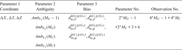
 $d_{br,\phi }^{k(C_{2})j(G_{1})}$ are the corresponding system biases related to the reference satellite and different frequencies. When M G GPS satellites and M C BDS satellites are observed, there will be 4 × MG – 1 + 4 × MC DD observations and 2 × MG – 1 + 2 × MC + 3 + 6 unknown parameters (coordinates, ambiguities, and biases), as shown in Table 2.
Classification of the unknown parameters for the new GPS and BDS combined RTK model.

The observation weight is determined in the same manner as the traditional approach using measurement noise. With Equation (7) and the weight matrix, least squares can be used for parameter estimation to obtain float solutions. The unknown parameters are the baseline components, the DD ambiguities and the additional biases. As the DD ambiguities also retain integer features, ambiguity resolution can be employed to obtain the final fixed solutions for the new approach. Because of additional biases in the new approach, the parameter estimation is slightly different from the traditional approach, as discussed below.
2.2.1. Approach regarding the change of reference satellite
For different systems and different frequencies, the new approach only uses one common reference ambiguity, for example, that of GPS L1, thus the parameter estimation approach is different. It can be divided into two types as follows:
Case one: the GPS reference satellite is not changed. In this case, the system biases are estimated as constants, and the DD ambiguities are also estimated as constants during a continuous period. Both should be re-initialised when a cycle slip occurs.
Case two: the GPS reference satellite is changed. In this case, all the system biases are re-initialised and also estimated as constants during the new period. The DD ambiguity  $N_{br}^{k(G_{1})j(G_{1})}$ is also re-initialised and the other DD ambiguities,
 $N_{br}^{k(G_{2})j(G_{1})}$,
 $N_{br}^{k(C_{1})j(G_{1})}$ and
 $N_{br}^{k(C_{2})j(G_{1})}$ are also estimated as constants.
2.2.2. Data processing
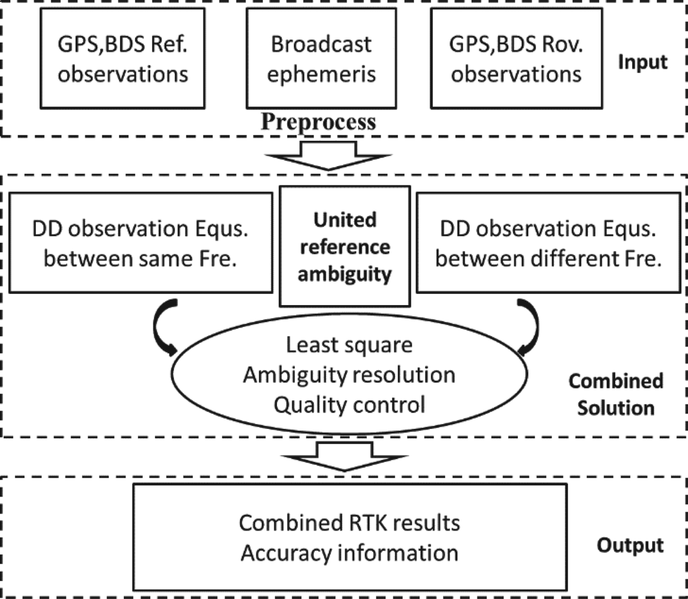
The data process is shown in Figure 1. It can be divided into three parts. The first part is input. Observations at the reference/rover stations and the broadcast ephemeris in real-time are first collected and pre-processing is then completed to obtain clean datasets. The second part is the combined RTK solution. Using the selected common reference ambiguity, it can form DD observation equations not only between the same frequencies, but also between different frequencies. Thus, least squares can be used for parameter estimation and quality control (deleting the poor data or reducing the weight of the poor data) to obtain the combined solution. The third part is output, combining RTK results and the accuracy information in real time.
Process flow of the combined RTK algorithm using one common reference ambiguity (“Ref.” represents the reference station and “Rov.” represents the rover station).

3. VALIDATION AND RESULTS
Real GNSS observation datasets were used for validation. The new approach was evaluated using the position accuracy and the observation residuals. Meanwhile, the system and frequency biases and the change of the reference ambiguities were also analysed and are discussed.
3.1. Datasets
The GNSS observation datasets were collected on day 279 in 2016. The antenna type was an HG-GOYH7151 (made by the HiGN GAIN company of China) and the receiver type was a UR380 (made by the UNICORE company of China). The receiver can track both GPS and BDS signals; the sampling rate was 1 s. The stations were in Xi'an in ShaanXi province. The distance between the reference and the rover station was 2.8 km. The observation time was from UTC 02:00:00 to 03:00:00. The data solution used the broadcast ephemeris.
3.2. The satellite numbers and Geometric Dilution of Precision values
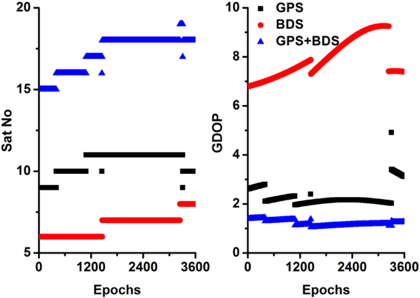
Figure 2 shows the observed satellite numbers. The mean satellite numbers are 10.3, 6.9 and 17.2 for the GPS, BDS and their combination, respectively. The average Geometric Dilution of Precision (GDOP) values were 2.4, 7.9 and 1.2 for GPS, BDS and their combination, respectively.
Numbers and GDOP values of the observed GPS and BDS satellites during the test period.

3.3. Analysis of position accuracy
The collocated data were processed using the new approach. Ambiguity resolution also used the popular Least-squares AMBiguity Decorrelation Adjustment (LAMBDA) strategy and was checked by ratio test (Teunissen, Reference Teunissen1995). The reference coordinates of these stations were calculated using static GPS Precise Point Positioning (GPS-PPP) of three days of observations (Zumberge et al., Reference Zumberge, Heflin, Jefferson, Watkins and Webb1997). The precision was better than 5 mm and 10 mm in the horizontal and vertical components, respectively, and can be used as reference values for accuracy analysis (Tu et al., Reference Tu, Ge, Huang and Zhang2013).
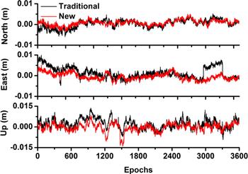
Figure 3 shows a comparison of the position biases between the traditional approach and the new method, respectively. The Root Mean Square (RMS) values improved from 2.9, 3.6 and 4.5 mm to 2.0, 2.5 and 3.2 mm in the north, east and up components, respectively. The results were consistent with previous RTK studies (Zhang et al., Reference Zhang, Guo and Meng2011b; Gao et al., Reference Gao, Gao, Pan, Qiao and Zhao2015), which means the new approach's position results were good.
Comparison of the position errors between the traditional approach and the new approach for one-hour data (from top to bottom, the north, east, and up components, respectively).

In addition, the accuracy of the new approach was also assessed using other datasets. The datasets were collected on day 301 and 303 in 2017. The stations were located in LinTong in ShaanXi province. There was a short baseline (several metres) between stations “NT01” and “NT02”, the sample rate was 30 s and both GPS and BDS signals were tracked. The antenna type was a Trimble NetR9 and the receiver type was an RNG80971.00.
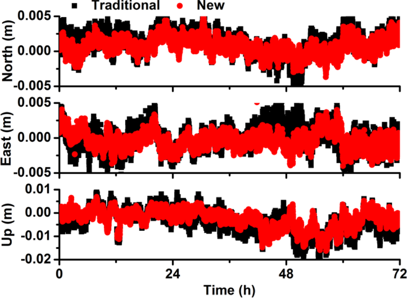
Figure 4 shows a comparison of the position bias between the new approach and the traditional approach for GPS and BDS combined RTK for three days of data. The statistical results show that the precision of the new approach is slightly better, especially in the east and vertical components. The mean RMS improved to 0.5, 0.7 and 1.1 mm in this test for the north, east and up components, respectively.
Comparison of the position error between the traditional approach and the new approach for three days of data (from top to bottom, the north, east, and up components, respectively).

3.4. Analysis of observation residuals
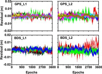
In addition, observation residuals can directly reflect position error. Figure 5 shows the residuals of the carrier phase observation. It can be seen that most of the DD residuals were smaller than 5 mm, and the largest residuals were smaller than 2 cm. For the new approach, as it used one common reference ambiguity, this will add new system and frequency biases. From these observation residuals, it can be seen that these system and frequency biases were precisely estimated.
Residuals of the carrier phase observations (different colours represent different satellites).

3.5. Analysis of system biases
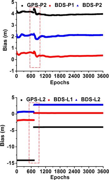
Figure 6 shows the time series of the estimated system and frequency biases. Here the dashed rectangle represents the change in the reference ambiguity. It can be seen that these biases were very stable during each continuous period except for the change in the reference ambiguity.
Time series of the estimated system and frequency biases (the dashed rectangle represents the change of the reference ambiguity).

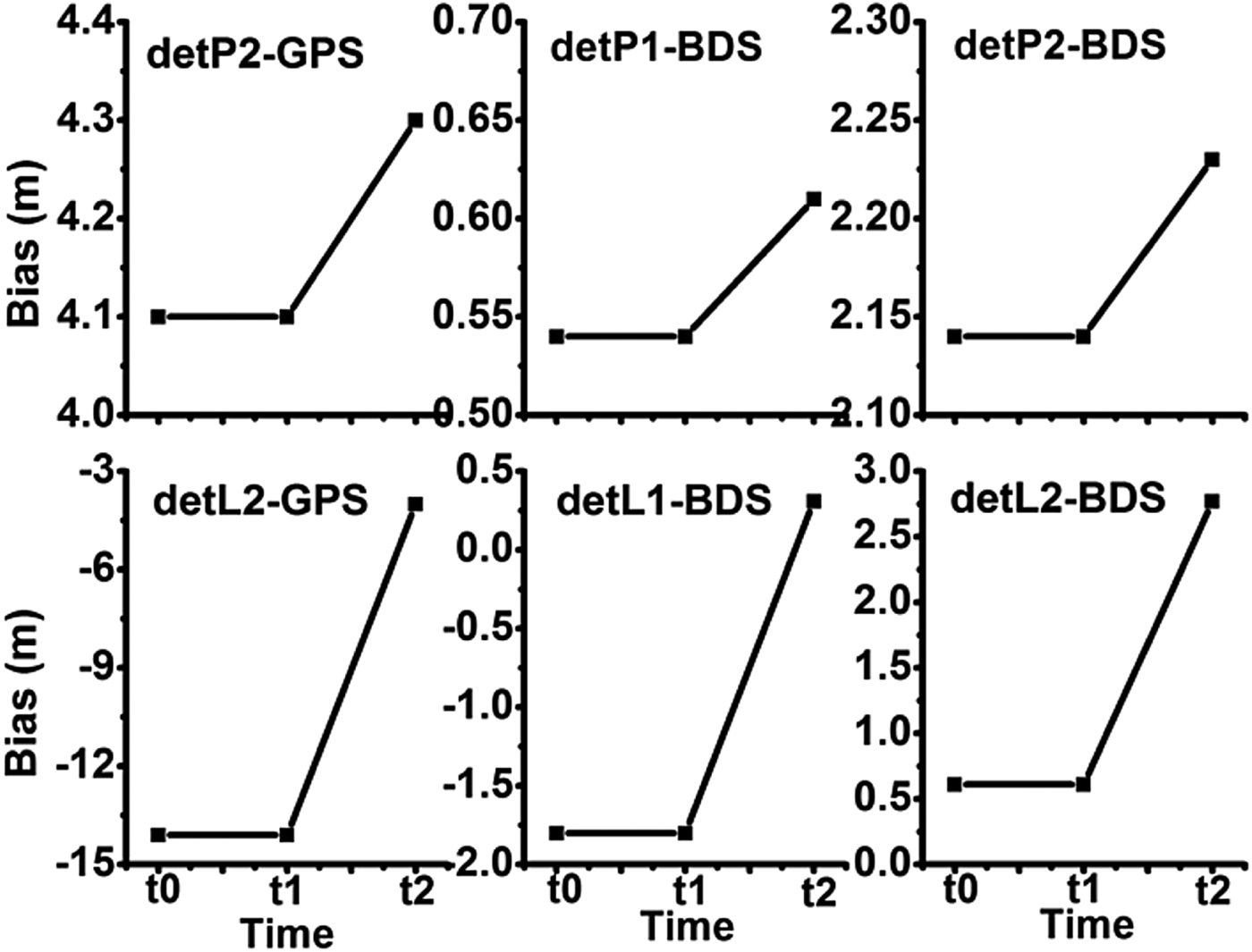
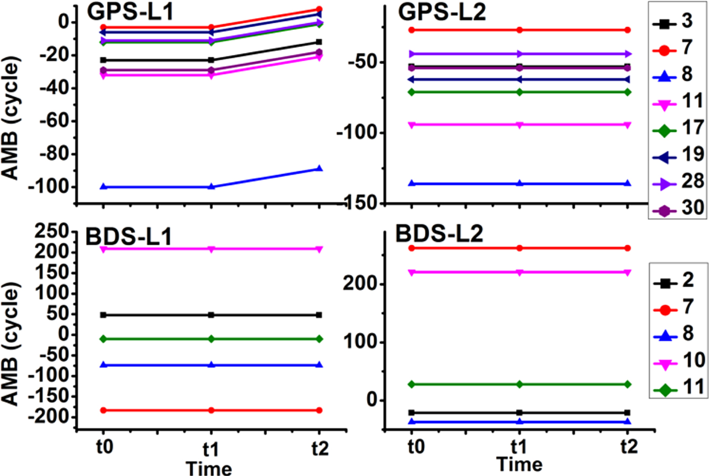
In addition, Figure 7 shows the details of the system and frequency bias changes due to the change in the reference ambiguity. Here, t 0 is the last epoch, t 1 is the current epoch which has the same reference ambiguity as t 0 and t 2 is the next epoch during which the reference ambiguity is changed. From t 0 to t 1, which refers to a continuous period where the reference ambiguity does not change, all the biases, whether for the pseudo-range or carrier phase, are constant. Thus, for parameter estimation, these system biases can be treated as constants. From t 1 to t 2, as the reference ambiguity changed, the estimated biases also changed; thus, in this condition, the parameters of the biases should be re-initialised.
Change in the system and frequency biases while the reference ambiguity changed (t 0, t 1, and t 2 represent the last period, the continuous period, and the change of reference ambiguity period).

3.6. Analysis of the ambiguity resolution
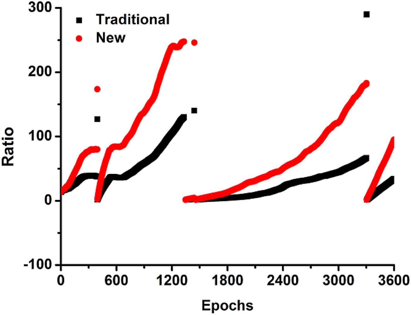
In the new approach, DD ambiguities can be solved as integers using LAMBDA only because these biases were precisely estimated or mitigated. Figure 8 shows the comparison of the ratio. It can be seen that the ratio values of the new approach are much larger than those of the traditional approach. The success rate and correct-fixing rate of the ambiguity resolution were also assessed. The statistical results of the one-hour experiment data show that the success rate is 100% and the correct-fixing rate is 100%. These results show that the modelling and estimation of these additional biases is reasonable.
Comparison of the ratio values between the traditional approach and the new approach.

3.7. Analysis of the change of the reference satellite
Figure 9 shows the time series of the estimated ambiguities. From t 1 to t 2, as the reference ambiguity changed, the estimated GPS L1 ambiguity also changed and all of the other ambiguities (GPS L2, BDS L1, and BDS L2) did not change. This was consistent with the parameter estimation strategy.
Changes of the estimated ambiguities while the reference ambiguity changed (t 0, t 1, and t 2 represent the last period, the continuous period, and the change of the reference ambiguity period).

4. CONCLUSION AND DISCUSSION
This paper has developed a model for GPS and BDS combined RTK by using one common reference ambiguity. Compared to the traditional combined RTK model that used separated reference ambiguities, this approach used the same reference ambiguity, and estimated pseudo-range and carrier phase system and frequency biases. Thus, it increased the strength of the combined model, and solved the problem of a frequently changing reference satellite. From the validation of the experimental data, several conclusions can be made:
• For the new combined RTK method, the position accuracy is slightly improved as compared to that of the traditional approach, especially in the east and vertical components.
• For the new combined RTK method, the main contribution is that it readily addresses the change of the reference satellite. It only needs to select the GPS L1 reference ambiguity, and does not need to consider the GPS L2, BDS L1, and BDS L2 reference ambiguities.
• Using one common reference ambiguity, it is necessary to introduce some new parameters, such as the pseudo-range and carrier phase biases of the selected reference satellite. These parameters should be re-initialised when the reference ambiguity changes.
• The estimated DD ambiguity parameters (GPS L1) are affected by the change of the reference ambiguity, and the other DD ambiguity parameters (GPS L2, BDS L1, and BDS L2) are not affected by the change of the reference ambiguity.
• As all of the carrier phase observations used one common reference ambiguity in the new approach, they established a relationship between the different systems and frequencies, increasing the strength of the combined model.
In this paper, the combined RTK model was only validated using GPS and BDS. More tests should be completed for the other GNSS systems, such as the GLONASS and Galileo systems. In addition, more tests should be completed for long-distance RTK.
ACKNOWLEDGMENTS
This work was partly supported by the program of National Natural Science Foundation of China (Grant No:41504006, 41674034), National Key Research and Development Plan of China (Grant No:2016YFB0501804) and Chinese Academy of Sciences (CAS) programs of “Pioneer Hundred Talents” (Y620YC1701), “Key Research Program of Frontier Sciences” (Grant No: QYZDB-SSW-DQC028).