Introduction

Non-linear iteration schemes are essential for a fast and stable solution of higher-order ice-flow models (HOIFMs). HOIFMs incorporate mechanical effects not present in the zeroth-order shallow-ice approximation of the governing equations (e.g. Reference HutterHutter, 1983). Mostly, this implies the inclusion of longitudinal deviatoric-stress gradients (e.g. Reference HindmarshHindmarsh, 2004). The topic of non-linear iteration schemes for HOIFMs is gaining attention as more and more numerical ice-sheet models include (or are planned to include) higher-order mechanics. Reference Hindmarsh and PayneHindmarsh and Payne (1996) proposed the unstable manifold correction (UMC) as a way to stabilize the numerical solution of implicit finite-difference discretizations of the time-dependent thickness-evolution equation for ice flow. Since 2002, Pattyn (e.g. Reference Pattyn2002, Reference Pattyn2003) has used the UMC in a Picard iteration to facilitate the solution of the velocity field in HOIFMs. In more recent work, a variant of the original UMC algorithm has been used (e.g. Reference Pattyn, De Smedt and SouchezPattyn and others, 2004; Reference PattynPattyn, 2008). Below, we demonstrate that, when using a proper HOIFM implementation, neither the original algorithm nor its variant should be used. Instead, we present a new, more appropriate, stable and simple algorithm that speeds up the iterative solution of the velocity field in HOIFMs for problems with real data.

Under- and Overshooting

The UMC is a relaxation-scheme feature for the numerical solution of a set of non-linear equations. Below, we use a model which, after discretization, results in the matrix form A(U)U = B. The common approach for solving such a model is to iteratively update a first guess U ⁰. This type of iterative update procedure is called a relaxation scheme. The simplest relaxation scheme is the true Picard iteration and consists of solving A(U^{γ− 1})U^γ = B for γ = 1,2,… until convergence. Relaxation schemes like the true Picard iteration can have several drawbacks (Fig. 1). On the one hand, when successive correction vectors, C^{γ− 1} = U^γ − U^{γ− 1} and C^γ = U^{γ +1} − U^γ , are in roughly the same direction, the scheme is undershooting. This means C^{γ− 1} could have been taken larger, so that fewer iterations and less computing time would be required to solve the equations. In such a case, one may obtain a faster convergence by overrelaxation, i.e. taking instead of C^γ a larger step μC^γ with μ > 1. On the other hand, if C^γ is in roughly the opposite direction to C^{γ− 1}, the scheme is overshooting the solution. At best, overshooting only slows down the solution process. At worst, an endless sequence of correction vectors shooting back and forth over the actual solution may arise. Overshooting can be remedied by underrelaxation, i.e. taking a smaller step, μC^γ with 0 < μ < 1.

Fig. 1.

Illustration of (a) undershooting and (b) overshooting for a sequence of iterates, U^{γ− 1}, U^γ and U^{γ +1}, and corresponding correction vectors, C^{γ− 1} and C^γ .

The Unstable Manifold Correction

Reference Hindmarsh and PayneHindmarsh and Payne (1996) proposed the UMC as a way to remedy the overshooting nature of relaxation schemes used to solve the non-linear thickness-evolution problem. Here we present a rigorous description of their method (as we understand it).

Consider an iterative solution method for a set of nonlinear equations which generates a sequence of approximate solutions,…, U^{γ− 2} = U^{γ− 3} + C^{γ− 3}, U^{γ− 1} = U^{γ− 2} + C^{γ− 2}, … Let be a preliminary (e.g. true Picard) iterate computed from U^{γ− 1} and let be the corresponding preliminary correction vector. Reference Hindmarsh and PayneHindmarsh and Payne (1996) observed that, if this preliminary iterate is accepted as the new iterate U^γ , once the time-step used in their calculations exceeds a certain threshold, after a few iterations, an endless sequence of overshooting along the same line in correction space occurs. Here they make the arguable assumption that the true solution lies on the overshooting line, which leads to

with E^{γ− 2} and E^{γ− 1} the true errors in approximations U^{γ− 2} and U^{γ− 1}, respectively (Fig. 2). Moreover, Hindmarsh and Payne use the (again arguable) assumption that the last accepted and the preliminary next correction step along the overshooting line are proportional to the true error (with equal proportionality) so that

From Equations (1) and (2), it follows that

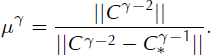
Hence,

(For all norm calculations in this paper, we use the square root of the sum of squares.) This allows us to compute a modified correction vector

called the UMC. The corrected approximation U^γ = U^{γ− 1} + C^{γ− 1}. As soon as the angle θ between successive correction vectors becomes ≥ 5π/6, Reference Hindmarsh and PayneHindmarsh and Payne (1996) apply the UMC. Note, however, that the more θ deviates from π, the poorer the validity of Equations (1) and (2). When θ < 5π/6 or , which implies can be calculated from

Fig. 2.

Illustration of overshooting along the same line in correction space for a sequence of approximate solutions, U^{γ− 2}, U^{γ− 1} and U^γ , the true solution, U ^true, the true error vectors, E^{γ− 2} and E^{γ− 1}, and the correction vectors, C^{γ− 2} and C^{γ− 1}. Here it is assumed that U ^true lies on the overshooting line.

Lessons from a Laminar-Flow Experiment

By adding the UMC to a true Picard iteration in a two-dimensional (2-D; Reference PattynPattyn, 2002) and a three-dimensional (3-D; Reference PattynPattyn, 2003) HOIFM implementation, a slightly stabilizing effect on the numerical solution of the velocity field was obtained. This is because, when using only a true Picard iteration, the successive approximations from these implementations show an overshooting of the actual solution (e.g. see Fig. 3a). We illustrate this for an infinite parallel-sided slab of isothermal ice on a uniform slope, α. We consider the ice frozen to the bed and take the x axis along the slope (positive downwards) and the z axis perpendicular to the slope (positive upwards). For this set-up and under the assumption of a steady flow, flow should be laminar, with velocity in the direction of the x axis given by (e.g. Reference PatersonPaterson, 1994)

where we take the flow-rate factor A = 10 ^{− 16} Pa ^{− 3} a⁻¹, the ice density ρ = 900 kg m ^{− 3}, the gravity constant g = 9.81 m s ^{− 2}, the slope α = 5°, and the ice thickness H = 200 m; s is the z coordinate of the surface. In Figure 3 we show successive approximations to the surface velocity for two 2-D HOIFM implementations and compare them to the exact solution (Equation (7)). Both implementations use the same LMLa (multilayer longitudinal stresses) flowline model (Reference HindmarshHindmarsh, 2004)

with effective viscosity

and Glen flow-law exponent n = 3. The boundary conditions are a traction-free surface, a no-slip condition at the base and, to enforce infinity of the slab, periodic boundary conditions (with an initial guess of zero velocity) at the left and right side of the domain. The slab is modelled over a 10 km domain length. The first implementation (I1) is based on a finite-difference discretization (Reference PattynPattyn, 2002). The second implementation (I2), which is being prepared for publication, is based on a finite-element discretization. We repeat the experiment using I2 since (in contrast to I1) it does not suffer from convergence problems, so it is properly suitable for evaluating the usefulness of the UMC in a Picard iteration for the numerical solution of the HOIFM. Moreover, its results match the exact solution given by Equation (7), as shown in Figure 3, are in line with theory when longitudinal deviatoric-stress gradients play a role and are internally consistent. I1 and I2 participated in the Ice-Sheet Model Intercomparison Project–Higher-Order ice-sheet Model (ISMIP-HOM) benchmark experiments (Reference PattynPattyn and others, 2008) with a variant of Equation (8) (i.e. the HOIFM Equations (11) and (9) for which the x axis (z axis) is chosen horizontal (vertically upwards). For the parallel-sided slab experiment, I1 and I2 use the true Picard iteration and 101 evenly spaced gridpoints in the x direction to solve the linearized model equations. As for all experiments in this paper, the computational domain is rectangular with 41 gridpoints in the z direction (irregularly spaced with decreasing grid distance towards the bed), the initial guess for the effective viscosity η ⁰ = 10⁶ Pa a over the whole domain, the initial correction vector C ⁰ = U ¹ (which implies U ⁰ = 0 m a⁻¹ over the whole domain) and we use a preconditioned conjugate-gradient solver (e.g. Reference BarrettBarrett and others, 1994) for the linear system. For I2, the norm of the residual of the preconditioned linear system is always <10 ^{− 5} for each non-linear iteration, which shows the preconditioned conjugate-gradient solver is capable of finding the actual solution for the linearized model and does not diverge.

Fig. 3.

Successive true Picard approximations of the surface velocity for an infinite parallel-sided slab of isothermal ice on a sloping bed (see text for details). Results are given for (a) a finite-difference implementation (Reference PattynPattyn, 2002) and (b) a finite-element implementation. Numbers on the curves correspond to iteration numbers. The thick grey line gives the exact solution.

For I1 and I2, we see a gradual update of the surface velocity, with the left and right sides of the domain lagging somewhat due to the periodic boundary conditions and the zero-velocity initial guess at the left and right boundaries (Fig. 3). Note that the successive approximations from I1 exhibit oscillations, causing the true Picard iteration to shoot back and forth over the exact solution. A future paper will address the causes of these oscillations and implications for the robustness of I1. Preliminary findings suggest the oscillations are due to the discretization scheme (e.g. the use of a non-staggered grid). Another explanation may be found in the unphysical smoothness and the lack of spatial variability in the experiment described above. No inhomogeneities are present whose (random) local oscillations could prevent or delay the onset of global instabilities (compare the speed-enhancing micro-scale roughnesses of shark’s hide, champion swimsuits and golf balls). In an attempt to stabilize the numerical solution of I1, and a largely similar implementation of a 3-D HOIFM, the UMC was introduced in a true Picard iteration and applied when θ ≥ 5π/6 (Reference PattynPattyn, 2002, Reference Pattyn2003). This offered only some slight stabilization and could not remove the oscillations in the successive velocity approximations.

The successive approximations of I2 contain no oscillations and converge steadily towards the exact solution (Fig. 3b). From the successive-approximation sequence, it is clear that the true Picard iteration is always undershooting (with θ always ≤π/10). This undershooting tendency of the true Picard iteration is confirmed by a wide range of other experiments (some of which are listed in Table 1). In only a few of these experiments, and mostly only in few iterations, do we observe an overshooting (θ ≥ 5π/6). Reference Picasso, Rappaz, Reist, Funk and BlatterPicasso and others (2004), who also used a 2-D finite-element LMLa model and a true Picard iteration to model glacier flow, found that no underrelaxation was necessary to obtain convergence. Moreover, Reference Colinge and RappazColinge and Rappaz (1999), using a similar model for 2-D flow in an infinite parallel-sided slab of ice, found that overrelaxation reduces the number of non-linear iterations by ∼30% for n = 3. These findings show that the main problem is undershooting and that the original UMC is of limited use in a Picard iteration for the numerical solution of the velocity field in this HOIFM, and presumably in others.

A Variant of the Original Unstable Manifold Correction Algorithm

In more recent work, the UMC was applied only when θ ≤ 5π/6 (e.g. Reference Pattyn, De Smedt and SouchezPattyn and others, 2004; Reference PattynPattyn, 2008). Note that this comes down to a violation of the reasoning behind the UMC. Nevertheless, the variant results in a considerably faster solution process (fewer iterations needed) than when using the true Picard iteration although, just like the original algorithm, it cannot remove the oscillations in the approximations. The variant reduces the amount of iterations since, provided and , then, first, when 3π/4 ≤ θ ≤ 5π/6, Equation (4) will result in an underrelaxation step and, secondly, when θ ≤ π/4, provided , Equation (4) will result in an overrelaxation step. In these cases, the variant makes sense. However, in most other cases Equation (4) will result in an undesirable over- or underrelaxation step. Moreover, a potentially beneficial underrelaxation step is missed when θ > 5π/6. Finally, problems with too large a multiplier μ may occur if the denominator in Equation (4) is too small (or, worse, zero).

A New Relaxation Scheme

Instead of the UMC and its variant, we propose a simple and (for all our experiments) stable relaxed Picard iteration , where

The range of θ for which we apply over- and underrelaxation and the corresponding value of μ were determined experimentally to minimize the number of iterations. We observed that taking a larger over- or a smaller underrelaxation step (e.g. μ = 4 or 1/3) may result in a divergence. Although it rarely happens that θ ≥ 19π/20, it is beneficial to take an underrelaxation step in such a case. We also experimented with an overshooting correction following the original UMC, but results were slightly less satisfying (more iterations needed) than when using Equation (10). This new scheme is very likely to also work for other HOIFM implementations, given the similar (elliptic) nature of the governing equations, and we encourage its application.

The proposed scheme substantially reduces the number of iterations required as compared to the true Picard iteration, especially for experiments with real data (Table 1; all experiments without periodic boundary conditions use real data). The same, however, is true for the variant of the UMC added to the true Picard iteration. Although the variant is theoretically less sound, it performs almost as well as, and in some cases even better than, the proposed scheme. However, the latter performs faster in almost all cases with real data. For these cases, a series of extra experiments (results not shown) with no slip (A = A _tuned, β ² = ∞) and high slip , low deformation and high deformation , indicate that these conclusions are fairly robust with respect to the tuning parameters β ² and A. For all experiments in Table 1, except for the parallel-sided slab experiment, we used a variant of Equation (8) for which the x axis (z axis) is chosen horizontal (vertically upwards). This results in the HOIFM

For all experiments in Table 1, the iteration procedure was stopped when

We use a small tolerance, φ ^tol = 10⁻⁶, to allow for a larger number of iterations and, thus, a better comparison between different relaxation algorithms. In general, a tolerance of 10⁻⁴ suffices to keep the associated truncation error below the discretization error, (propagated) measurement errors and the likely model error. Using φ ^tol = 10⁻⁴ would not alter the conclusions that can be drawn from Table 1.

Table 1.

Number of non-linear iterations needed for the numerical solution of HOIFMs given by Equations (8) and (9) and Equations (11) and (9) with a traction-free surface boundary condition and a basal boundary condition , with τ _b the basal drag and b the basal elevation using a finite-element implementation. Results are given for the true Picard iteration (TPI), the relaxed Picard iteration proposed in this study (RPI) and the variant on the original UMC algorithm (Reference Hindmarsh and PayneHindmarsh and Payne, 1996) used by Pattyn in a Picard iteration (UMP). Calculations were performed along a flowline for a parallel-sided slab (PSS) (see text for details); ISMIP–HOM (I-H) experiments B, D, E1 (no sliding) and E2 (sliding spot) (Reference PattynPattyn and others, 2008); Sofiyskiy glacier (SFG), Russia; Pine Island Glacier (PIG), West Antarctica; McCall Glacier (MCG), Alaska, USA; Storglaciären (STG), Sweden; John Evans Glacier (JEG), Canada and Hintereisferner (HEF), Austria. Given also are the number of gridpoints (evenly spaced) in the x direction, m, the numerical domain length, L, the flow-rate factor, A, the ice density, ρ, the type of basal boundary condition (BBC), the use of periodic boundary conditions (PBC) and the data source. ‘l.s.l.’ denotes the use of a linear sliding law: τ _b = u _b β ² with u _b the basal velocity and β ²(x) a positive basal-friction coefficient.

Conclusions

The above analysis demonstrates that neither the UMC nor its variant should be used in a Picard iteration to solve the velocity field in HOIFMs. The original UMC algorithm is not useful since it corrects only for overshooting, whereas undershooting is the main problem in the solution of the velocity field in HOIFMs. Although the variant of the original algorithm performs rather well in our experiments, it is theoretically less sound and can potentially lead to unnatural under- or overrelaxation steps. Instead, we propose a new simple and stable Picard-relaxation scheme that results in a fast solution of the velocity field in HOIFMs, especially for problems with real data. Given the similar (elliptic) nature of HOIFMs, the new scheme should perform well in other HOIFM implementations and we encourage its application.