1. Introduction
The evaporation of droplets has captivated the attention of researchers increasingly, owing to its ubiquity and pivotal role in various industrial applications such as inkjet printing (Talbot et al. 2017), medical diagnosis (Thieret Reference Thieret2008), DNA mapping (Jing et al. Reference Jing1998) and surface patterning (Harris et al. Reference Harris, Hu, Conrad and Lewis2007). Droplet vibrations have also emerged as a prominent area of interest among researchers. Dating back to the seminal work of Rayleigh (Reference Rayleigh1879), early studies revealed that a free spherical-cap drop (referring to its geometric shape of uniform surface curvature), constrained by surface tension, undergoes oscillations around its equilibrium shape at a characteristic frequency. Subjected to different mechanical excitations (Noblin et al. Reference Noblin, Buguin and Brochard-Wyart2005, Reference Noblin, Kofman and Celestini2009; Vukasinovic, Smith & Glezer Reference Vukasinovic, Smith and Glezer2007; Ding et al. Reference Ding, Zhu, Gao and Lu2018), droplets may exhibit a variety of interesting shapes, which could have potential applications in microfluidics. These applications include drop-on-demand printing (Basaran, Gao & Bhat Reference Basaran, Gao and Bhat2013; Ding & Bostwick Reference Ding and Bostwick2022; Lohse Reference Lohse2022), nanopatterned wafer cleaning (Xu et al. Reference Xu, Vereecke, Van den Hoogen, Smeers, Armini, Delande and Struyf2013) and biomimetic surface design (Lafuma & Quéré Reference Lafuma and Quéré2003). In most inkjet printing scenarios, the deposition pattern of droplets is largely influenced by the evaporation of ink droplets. However, the evaporation dynamics of non-spherical droplets differs significantly from that of common spherical-cap droplets. Therefore, it is crucial to consider the evaporation process of non-spherical droplets.
To effectively control and comprehend the evaporation process, it is essential to employ an appropriate model that is capable of predicting the evaporation flux of liquid from the free surface of a droplet into the surrounding atmosphere. The diffusion-limited model, pioneered by Mangel & Baer (Reference Mangel and Baer1962), stands as the most widely studied and simplest model for describing the evaporation flux. In the recent review by Wilson & D’Ambrosio (Reference Wilson and D’Ambrosio2023), the diffusion-limited model was discussed in great detail, and several classic solutions regarding droplet evaporation flux derived from this model were presented. In the diffusion-limited model, the vapour concentration conforms to Laplace’s equation. Given that the time taken for vapour to diffuse away from the free surface of the droplet is significantly shorter than the droplet’s lifetime, the diffusion process can be regarded to be quasi-static (Wilson & D’Ambrosio Reference Wilson and D’Ambrosio2023). Even with this assumption, solving Laplace’s equation for vapour concentration analytically proves challenging, let alone determining the internal flow of the droplet driven by the evaporation flux. For the sake of simplifying the internal flow analysis, Boulogne, Ingremeau & Stone (Reference Boulogne, Ingremeau and Stone2017) introduced a method where a droplet is situated within a large hydrogel bath. Under this set-up, the evaporation flux can be well approximated as being spatially uniform, often denoted as the spatially uniform evaporation. D’Ambrosio et al. (Reference D’Ambrosio, Wilson, Wray and Duffy2023) provided a comprehensive study of how evaporative fluxes (including both diffusion-limited and spatially uniform fluxes) affect the flow within and deposition from an evaporating sessile droplet. Boulogne et al. (Reference Boulogne, Ingremeau and Stone2017) also conducted a comparison of the internal flow of droplets containing non-volatile solutes under these two models, and the results indicated that similar patterns were formed after complete evaporation of the droplets in both cases. This phenomenon of pattern formation is known as the ‘coffee ring’ effect.
The ‘coffee ring’ effect, first studied by Deegan et al. (Reference Deegan, Bakajin, Dupont, Huber, Nagel and Witten1997, Reference Deegan2000), refers to a deposition pattern that is darkest towards its edge. It is now well-established that the gathering of particles at the contact line stems from an outward radial flow caused by evaporation and a pinned contact line. As the volatile liquid evaporates, the solvent at the pinned contact line needs replenishment, thereby inducing radial liquid flow. To provide further elucidation on this phenomenon, a more comprehensive solution incorporating both the width of the ring and the jamming effect was proposed (Popov Reference Popov2005). Ozawa, Nishitani & Doi (Reference Ozawa and Nishitani2005) expanded upon the diffusion-limited model by considering variations in evaporation flux and viscosity with solute concentration. Their numerical results demonstrated a transition in the deposition pattern from dot-type to ring-type as the initial concentration of solute increased. The deposition of a droplet with a receding contact line was investigated, revealing a mountain-like pattern under the assumption of the spatially uniform evaporation (Freed-Brown Reference Freed-Brown2015). In this process, the contact angle remains constant, defining what is known as the constant contact angle (CA) mode, as opposed to the pinned contact line, which characterises the constant contact radius (CR) mode (Wilson & D’Ambrosio Reference Wilson and D’Ambrosio2023). In practical scenarios, aside from these two modes, droplets frequently undergo evolution characterised by a variety of mixed modes, comprising diverse combinations of these two extreme models. The so-called stick-slide (SS) mode is the most commonly observed mixed mode, and multiple studies have focused on this mode (Bodiguel et al. Reference Bodiguel, Doumenc and Guerrier2009, Reference Bodiguel, Doumenc and Guerrier2010; Chen et al. Reference Chen, Suzuki, Mahara and Yamaguchi2012; Zigelman & Anna Reference Zigelman and Manor2016). Stauber et al. (Reference Stauber, Wilson, Duffy and Sefiane2014, Reference Stauber, Wilson, Duffy and Sefiane2015) gave thorough characterisations of the lifetimes of droplets evaporating in the CR, CA and SS modes, allowing for a clear understanding of the evaporation processes in each mode.
Due to the significant role of the flow within an evaporating droplet in the deposition process, numerous investigations have centred on this issue. These studies have relied on different flow models to derive final analytical or numerical results. Regarding the lubrication theory, Hu & Larson (Reference Hu and Larson2005) derived a semi-analytical solution. Fischer (Reference Fischer2002) pursued a numerical solution for viscous flow within the constraints of lubrication theory. Widjaja & Harris (Reference Widjaja and Harris2008) addressed the solution of Stokes flow across a range of contact angles, from zero to ninety degrees. Gelderblom, Bloemen & Snoeijer (Reference Gelderblom, Bloemen and Snoeijer2012) analytically solved the Stokes equations within a wedge geometry, allowing for any given contact angle. Furthermore, exact analytical solutions for inviscid flow were obtained for various geometries, including hemispheres (Tarasevich Reference Tarasevich2005), hemicylinders (Petsi & Burganos Reference Petsi and Burganos2005), and cylindrical caps (Petsi & Burganos Reference Petsi and Burganos2006). Masoud & Felske (Reference Masoud and Felske2009a ,Reference Masoud and Felske b ) utilised toroidal coordinates to obtain solutions for both inviscid flow and Stokes flow within sessile droplets.
The evaporation flux, the evaporation modes and the internal flow all contribute to the deposition patterns of drying droplets. Numerous studies have explored the mechanisms behind the various pattern formations observed in dried droplets. Hu & Larson (Reference Hu and Larson2006) were the first to account for Marangoni flow in the ‘coffee ring’ effect. Zheng (Reference Zheng2009) proposed the ‘pipe model’, which addressed the truncated transport process in deposition formation. Sefiane (Reference Sefiane2014) provided an extensive review of deposition patterns formed by various fluids, including ploymers, paints, biological fluids and nanoparticle suspensions. Thiele (Reference Thiele2014) focused on the role of the moving contact line in deposition formation. Parsa, Harmand & Sefiane (Reference Parsa, Harmand and Sefiane2018) presented a comprehensive review of experiments on the deposition patterns of drying droplets of complex fluids, while Thampi & Basavaraj (Reference Thampi and Basavaraj2023) highlighted key developments, emphasizing the principles governing drying drops and their resulting patterns.
Despite the simplicity of droplet geometry, typically resembling a spherical cap or flat disk, deriving analytical expressions to accurately describe the evaporation flux within the diffusion-limited model remains challenging. In the pioneering work of Deegan (Reference Deegan2000) and Popov (Reference Popov2005), toroidal coordinates were adopted to solve this mixed boundary value problem for Laplace’s equation due to its convenience in describing the spherical cap geometry. Popov (Reference Popov2005) addressed the boundary value problem for Laplace’s equation using Legendre functions of fractional degree, derived by Lebedev (Reference Lebedev1965). Through this approach, he obtained expressions for the evaporation flux of circular droplets with small contact angles, as well as for other specific contact angles.
However, compared to spherical-cap droplets, non-spherical droplets are more prevalent in nature, primarily due to the uneven structures of solid surfaces. Consequently, research on their evaporation is becoming increasingly popular in the academic community. Various complicated geometries of droplets have been studied, with particular attention paid to droplets on a slope experiencing deformation caused by gravity. Du & Deegan (Reference Du and Deegan2015) conducted numerical simulations to investigate the formation of contact line deposits resulting from the evaporation of a two-dimensional droplet on an inclined surface. Sáenz et al. (Reference Sáenz, Wray, Che, Matar, Valluri, Kim and Sefiane2017) established a universal scaling law for the evaporation rate applicable to droplets of specific non-spherical shapes through a combination of experimental observations and theoretical modelling. Timm et al. (Reference Timm, Dehdashti, Darban and Masoud2019) undertook a theoretical investigation into the total evaporation rate of a sessile droplet pinned on an inclined surface, initially focusing on determining the droplet shape. Wray & Moore (Reference Wray and Moore2023) updated and expanded upon certain aspects of the study conducted by Saenz et al. (Reference Sáenz, Wray, Che, Matar, Valluri, Kim and Sefiane2017). They first derived an analytical solution for the evaporation of non-circular droplets with high accuracy. They obtained an asymptotic expansion for the evaporative flux from the free surface of very thin droplets with a wavy contact line. The effect of gravity on oscillating droplets has also attracted much attention. Zhang, Zhou & Ding (Reference Zhang, Zhou and Ding2023) investigated the natural oscillations of sessile drops on a plane under gravity. However, during the oscillating process of droplets, many more complex geometric shapes may emerge, and the impact of these peculiar non-thin non-spherical shapes on droplet evaporation has not been well explored.
Some non-spherical-cap (i.e. wavy) droplets were observed in electrowetting (Oh, Ko & Kang Reference Oh, Ko and Kang2008). Electrowetting is a valuable tool for controlling the behaviour of droplets, and has been shown to suppress the coffee ring effect (Eral et al. Reference Eral, Augustine, Duits and Mugele2011) and reduce contact angle hysteresis (Li & Mugele Reference Li and Mugele2008). The shapes of these non-spherical-cap droplets can be expressed using Legendre polynomials, indicating that their curvature varies periodically with polar angle. Previous studies on the evaporation of non-spherical droplets (Sáenz et al. Reference Sáenz, Wray, Che, Matar, Valluri, Kim and Sefiane2017; Wray & Moore Reference Wray and Moore2023) have shown that the evaporation flux is enhanced at high-curvature regions. Similar non-spherical-cap droplets can also be observed in practical scenarios, such as in adjacent droplets (Wang et al. Reference Wang, Orejon, Takata and Sefiane2022) or in pendant droplets influenced by gravity (Slobozhanin & Alexander Reference Slobozhanin and Alexander2006) or an electric field (Ferrera et al. Reference Ferrera, López-Herrera, Herrada, Montanero and Acero2013). Notably, a convex–concave interface shape in an electric field was reported in the experiments conducted by Gubarenko et al. (Reference Gubarenko, Chiarot, Ben Mrad and Sullivan2008). Besides, based on the study by Zhou & Zhang (Reference Zhou and Zhang2017) on the three-plate system, placing annular plates with specific wetting properties on the surface of a hemispherical droplet can stabilise the droplet in a highly similar non-spherical-cap shape. This approach provides a potential method for obtaining stable non-spherical-cap droplets. Therefore, the evaporation of non-spherical-cap droplets is a highly significant research topic.
Previous research on evaporation (Picknett & Bexon Reference Picknett and Bexon1977; Deegan et al. Reference Deegan, Bakajin, Dupont, Huber, Nagel and Witten1997, Reference Deegan2000; Hu & Larson Reference Hu and Larson2005; Erbil Reference Erbil2012) has concentrated primarily on thin droplets. Nevertheless, there remains a gap in the literature concerning the investigation of non-thin non-spherical droplets. In this paper, our primary focus is on deriving analytical expressions for the evaporation flux of non-spherical-cap droplets and the inviscid flow within them, utilizing asymptotic analysis methods. There are several similarities between the droplet shapes in Wray & Moore (Reference Wray and Moore2023) and those in this paper; both are derived from a circle (sphere) and incorporate a small parameter to describe the deformation. Although one considers thin droplets and the other nearly hemispherical non-thin droplets, the asymptotic approach is expected to be effective for both. Inspired by Wray & Moore (Reference Wray and Moore2023), it is judicious to use the asymptotic analysis to address the evaporation problems of these non-spherical-cap droplets. The paper is organised as follows. In § 2, we provide a detailed demonstration of droplet shapes and formulate the mathematical model for evaporation. Subsequently, in § 3, we solve the problem and obtain an asymptotic expansion to describe the evaporation flux, which we validate to be in good agreement with numerical simulations. In § 4, we examine the inviscid flow under the spatially uniform evaporation, which can also be solved using asymptotic analysis and validated with original boundary conditions. Finally, we deduce the surface density profile of the droplet deposition, which can be obtained by solving a system of ordinary differential equations numerically, in § 5.
2. Problem formation
Consider a sessile droplet resting on a flat plate, characterised by a constant density
 $ \rho $
and a surface tension
 $ \gamma $
. The gravity is neglected. The surface of a droplet can be represented geometrically in the spherical coordinate system
 $(r,\theta,\varphi)$
. If we define the central point of a droplet as the origin, then the surface shape of the droplet can be expressed as
 \begin{equation} \overline{r}_{s}\left(\theta \right)=R\left[1+\varepsilon P_{n}\left(\cos \theta \right)\right],\quad \overline{r}\leq \overline{r}_{s},\ 0\leq \theta \leq \frac{\unicode{x03C0}}{2}\text{ and }0\leq \varphi \lt 2{\unicode{x03C0}} ,\text{ for }n=2,4,6,\ldots, \end{equation}
where R denotes the radius of the undeformed droplet,
 $ \varepsilon $
is the amplitude of the deformation, and P
n
signifies the Legendre polynomials of order n, and the shape of each droplet corresponds to the order n, which also represents the numbers of lobes in the shape (see figure 1). The lowest mode is associated with n = 2. Modes with n = 0 and n = 1 do not occur, as they would result in a deformed droplet that violates the volume conservation of the original spherical droplet and alters its centre of mass. Legendre polynomials are the eigenfunctions of the Laplace equation in axisymmetric spherical coordinates, and are orthogonal over the interval
 $(0,{\unicode{x03C0}})$
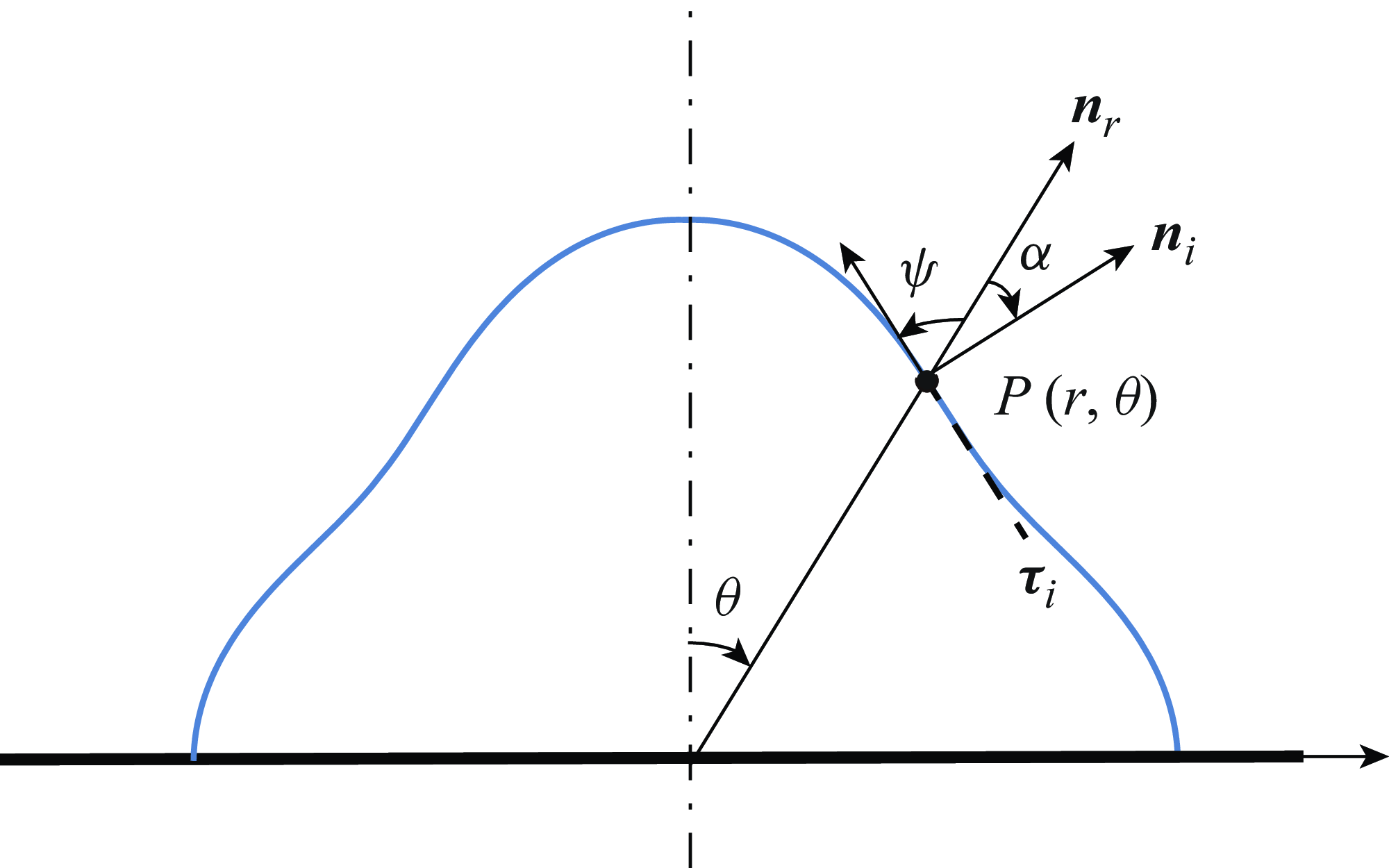
. Due to this orthogonality, any differentiable function defined in this interval can be expressed as a linear combination of Legendre polynomials, following the principles of spectral decomposition (Rade & Westergren Reference Rade and Westergren1999; Arfken & Weber Reference Arfken and Weber2005). Thus for axisymmetric droplet shapes (i.e. independent of the azimuthal angle), the surface can be expressed as a generalised Fourier series in terms of Legendre polynomials. Consequently, solving the evaporation problem for droplets with shapes like the one in (2.1) provides valuable insights for addressing the evaporation behaviour of other arbitrarily complex droplet geometries. We restrict the contact angle of the droplets to 90°, ensuring symmetry with respect to the substrate. Since their undeformed shape is hemispherical, this configuration results in a spatially uniform evaporation flux. As the odd modes do not exhibit such symmetry, only the even modes are relevant here, consistent with Oh et al. (Reference Oh, Ko and Kang2008). In practice, water droplets are often placed on a polystyrene substrate to achieve a contact angle close to 90° (Sharp, Farmer & Kelly Reference Sharp, Farmer and Kelly2011).
Side view schematics of droplet surface shapes represented by
 $\overline{r}_{s}(\theta )=R[1+0.2P_{n}(\cos \theta )]$
with (a) n = 2, (b) n = 4 and (c) n = 6, respectively. The droplets are axisymmetric, and the dot-dashed line, labelled as the ‘symmetry axis’, serves as the axis of rotation. The dashed line denotes the undeformed surface;
 $ \theta $
is measured clockwise.

When the rate-limiting process is the diffusion (i.e. the diffusion-limited model), the vapour concentration
 $\overline{c}$
satisfies Laplace’s equation. The evaporation flux at the liquid–vapour interface can be expressed as
 \begin{equation} \overline{J}=-\frac{D}{\rho }\frac{\partial \overline{c}\left(r,\theta \right)}{\partial \boldsymbol{n}_{{i}}}\quad\text{at }\overline{r}=\overline{r}_{s}, \end{equation}
where D is the diffusion coefficient for vapour in air, and
n
represents the unit normal vector directed into the gas phase. The boundary conditions dictate that the air along the surface of the drop is saturated with vapour, resulting in a constant value
 $\overline{c}_{s}$
. As the distance from the droplet increases, the variable
 $\overline{c}$
converges towards the ambient vapour concentration, denoted as
 $\overline{c}_{\infty }$
.
The physical parameters are non-dimensionalised as
 \begin{equation} r=\overline{r}/R,\quad c=(\overline{c}-\overline{c}_{\infty })/(\overline{c}_{s}-\overline{c}_{\infty }),\quad J=\rho R\overline{J}/[D(\overline{c}_{s}-\overline{c}_{\infty })], \end{equation}
where c is the dimensionless vapour concentration, and J is the dimensionless evaporation flux at the liquid–-vapour interface. Laplace’s equation in spherical coordinates can be written as
 \begin{equation} \Delta c=\frac{1}{r^{2}}\frac{\partial }{\partial r}\left(r^{2}\frac{\partial c}{\partial r}\right)+\frac{1}{r^{2}\sin \theta }\frac{\partial }{\partial \theta }\left(\sin \theta \frac{\partial c}{\partial \theta }\right)=0\quad\text{in }r\gt r_{s}. \end{equation}
Due to the rotational symmetry of the droplet, the azimuthal component of c is neglected. The boundary conditions are
 \begin{equation} c=1\text{ at }r=r_{s},\quad c\rightarrow 0\text{ as }r\rightarrow \infty . \end{equation}
Besides, the flux normal to the substrate is zero, indicating that vapour cannot penetrate the substrate, namely,
 \begin{equation} \frac{\partial c}{\partial \boldsymbol{n}_{{s}}}=0\quad\text{on the substrate}, \end{equation}
where
 $\boldsymbol{n}_s$
represents the unit normal vector pointing upwards from the substrate.
3. Evaporation flux
3.1. Asymptotic expansion solution
Consistent with Wray & Moore (Reference Wray and Moore2023), we select the amplitude of the deformation
 $ \varepsilon $
as the perturbation parameter, enabling us to express the vapour concentration as an asymptotic series
 \begin{equation} c\left(r,\theta ,\varepsilon \right)\sim c^{0}\left(r,\theta \right)+\varepsilon\, c^{1}\left(r,\theta \right), \end{equation}
and give the evaporation flux by
 \begin{equation} J\left(\theta ,\varepsilon \right)\sim J^{0}\left(\theta \right)+\varepsilon\, J^{1}\left(\theta \right)=\frac{\partial c^{0}\left(r,\theta \right)}{\partial \boldsymbol{n}_{{i}}}\Bigg|_{r={r_{s}}}+\varepsilon\, \frac{\partial c^{1}\left(r,\theta \right)}{\partial \boldsymbol{n}_{{i}}}\Bigg|_{r={r_{s}}} .\end{equation}
Substituting (3.1) into (2.2), we get
 \begin{equation} {\Delta} c^{0}+\varepsilon\, {\Delta} c^{1}=0 .\end{equation}
Since (3.3) holds for arbitrary values of
 $ \varepsilon $
, we have
 ${\Delta} c^{0}=0$
and
 ${\Delta} c^{1}=0$
. In other words, both c
0 and c
1 satisfy Laplace’s equation separately. Substituting (3.1) into (2.5) produces
 \begin{equation} c^{0}(r\rightarrow \infty ,\theta )=0,\quad c^{1}(r\rightarrow \infty ,\theta )=0, \end{equation}
 \begin{equation} c^{0}\left(r=r_{s},\theta \right)+\varepsilon\, c^{1}\left(r=r_{s},\theta \right)=1 .\end{equation}
Given that r
s
is a function of
 $ \varepsilon $
as well, the explicit dependence on
 $ \varepsilon $
in (3.5) has not been presented yet. This is attributed to the fact that
 $c^{0}(r=r_{s},\theta )$
and
 $c^{1}(r=r_{s},\theta )$
rely on
 $ \varepsilon $
via the variable r. To address this issue, we expand each term in a Taylor series to first order in
 $ \varepsilon $
around r = 1. Consequently, we can express (3.5) as
 \begin{equation} c^{0}\left(1,\theta \right)+\varepsilon\, c_{r}^{0}\left(1,\theta \right)P_{n}\left(\cos \theta \right)+\varepsilon\, c^{1}\left(1,\theta \right)+\varepsilon ^{2}\,c_{r}^{1}\left(1,\theta \right)P_{n}\left(\cos \theta \right)=1 .\end{equation}
Subsequently, we can group the coefficients of each power of
 $ \varepsilon $
and set them to zero. This condition is then transferred back to the undeformed surface r = 1:
 \begin{equation} c^{0}(1,\theta )=1,\quad c_{r}^{0}(1,\theta )\,P_{n}(\cos \theta )+c^{1}(1,\theta )=0. \end{equation}
Initially, we try to obtain c
0 from the Laplace equation
 ${\Delta} c^{0}=0$
. In our investigation, we consider fixed contact angle 90°, allowing us to transform this problem into the evaporation of hemispherical droplets. Given that the droplets exhibit symmetry with respect to the substrate, it is evident that the evaporation flux is uniform throughout; specifically,
 \begin{equation} J^{0}(\theta)=1\quad\text{at }r=1. \end{equation}
To derive the expression for
 $J^{0}(\theta )$
at the deformed surface r = r
s
, we also expand
 $c^{0}(r=r_{s},\theta )$
in a Taylor series, and represent it by two orthogonal components in polar coordinates:
 \begin{align} &J^{0}(\theta)={}\nonumber\\ & \! -\frac{\partial }{\partial r}\cos \alpha \!\left[\!c^{0}\! \left(r,\theta \right)+c_{r}^{0}\! \left(r,\theta \right)\varepsilon\, P_{n}\left(\cos \theta \right)+\cdots +\frac{c_{r}^{\left(m\right)}\left(1,\theta \right)}{m!}\varepsilon ^{m}\,P_{n}\left(\cos \theta \right)^{m}+\cdots \!\right]\!\Bigg|_{r=1}\nonumber\\[6pt] & \! -\frac{\partial }{\partial \theta }\sin \alpha \!\left[\!c^{0}\! \left(r,\theta \right)+c_{r}^{0}\! \left(r,\theta \right)\varepsilon\, P_{n}\left(\cos \theta \right)+\cdots +\frac{c_{r}^{\left(m\right)}\left(1,\theta \right)}{m!}\varepsilon ^{m}P_{n}\left(\cos \theta \right)^{m}+\cdots \!\right]\!\Bigg|_{r=1}, \nonumber\\\end{align}
where the subscript r indicates the derivative with respect to r, superscript numbers in parentheses represent the order of the derivative, and
 $ \alpha $
is the angle starting from the vector in the r direction
 $\boldsymbol{n}_r$
to the normal vector
 $\boldsymbol{n}_i$
of the surface (see figure 2). In polar coordinates, the angle between the tangent line on a curve and the line between the tangent point and the pole (see figure 2) can be expressed as
Definitions of the intersection angles
 $ \alpha $
and
 $ \psi $
. In polar coordinates, for a point P(r,
 $ \theta $
) of the curve, the normal vector at that point is
n
i
, the tangent vector is
 $ \unicode{x1D6D5} $
i
, and the vector in the direction of the line connecting the pole and the point P is
n
r
. The intersection angle
 $ \alpha $
of the point P is from the vector
n
i to the vector
n
r
, while the intersection angle
 $ \psi $
is from the vector
n
r
to the vector
 $ \unicode{x1D6D5} $
i
. As both
 $ \alpha $
and
 $ \psi $
start from
n
r
, and the direction of
n
r
is always between
n
i
and
 $ \unicode{x1D6D5} $
i
,
 $ \alpha $
and
 $ \psi $
are measured in opposite directions:
 $ \alpha $
is measured clockwise, while
 $ \psi $
is measured anticlockwise.

 \begin{equation} \tan \psi =\frac{r_{s}\left(\theta \right)}{r'_{s}\left(\theta \right)},\quad-\frac{{\unicode{x03C0}} }{2}\leq \psi \leq \frac{{\unicode{x03C0}} }{2}, \end{equation}
where
 $r'_{s}(\theta )$
represents the derivative of
 $r_{s}(\theta )$
with respect to
 $ \theta $
. We can determine the angle
 $ \alpha $
by
 \begin{equation} \cos \alpha =\frac{r_{s}\left(\theta \right)}{\sqrt{r_{s}\left(\theta \right)^{2}+r'_{s}\left(\theta \right)^{2}}},\quad \sin \alpha =\frac{r'_{s}\left(\theta \right)}{\sqrt{r_{s}\left(\theta \right)^{2}+r'_{s}\left(\theta \right)^{2}}}. \end{equation}
From (3.7a ) and (3.8), we can deduce that
 \begin{equation} \frac{\partial c^{0}\left(r,\theta \right)}{\partial \theta }\Bigg|_{r=1}=\frac{\partial ^{2}c^{0}\left(r,\theta \right)}{\partial \theta ^{2}}\Bigg|_{r=1}=0 .\end{equation}
Substituting (3.12) into Laplace’s equation yields
 \begin{equation} \frac{\partial ^{2}c^{0}\left(r,\theta \right)}{\partial r^{2}}\Bigg|_{r=1}=-2\frac{\partial c^{0}\left(r,\theta \right)}{\partial r}\Bigg|_{r=1}=2 .\end{equation}
In order to obtain higher-order derivatives of c
0 with respect to r, we can differentiate both sides of Laplace’s equation with respect to r. All terms with partial derivatives with respect to
 $\theta$
are equal to 0. This gives
 $c_{r}^{(3)}(1,\theta )=-2c_{r}^{(2)}(1,\theta )$
. The remainder of the process can be carried out in a similar manner, leading us to conclude that
 \begin{equation} c_{r}^{\left(m\right)}\left(1,\theta \right)=\left(-1\right)^{m}2^{m-1} .\end{equation}
With these conclusions, (3.9) becomes
 \begin{align} & J^{0}\left(\theta \right) = \cos \alpha -2\varepsilon\, P_{n}\left(\cos \theta \right)\cos \alpha +\varepsilon\, P_{n}'\left(\cos \theta \right)\cos \alpha +\cdots\nonumber \\ &=\!\sum _{m=0}^{\infty } \!\left\{\!\frac{\left(-2\right)^{m}}{m!}\varepsilon ^{m}\left[P_{n}\left(\cos \theta \right)\right]^{m}\cos \alpha -\frac{\left(-2\right)^{m-1}}{m!}\varepsilon ^{m}m\left[P_{n}\left(\cos \theta \right)\right]^{m-1}P_{n}'\left(\cos \theta \right)\cos \alpha \!\right\}\!. \nonumber \\\end{align}
Then we proceed to consider c 1. Given the solution for c 0, the boundary condition of c 1 (3.7b ) is expressed as
 \begin{equation} c^{1}\left(1,\theta \right)=P_{n}\left(\cos \theta \right) .\end{equation}
This Laplace’s equation with a Dirichlet boundary value problem can be readily solved using the method of separation of variables. Let us express the right-hand side of (3.16) using a Fourier–Legendre series expansion, also known as a generalised Fourier series expansion:
 \begin{equation} P_{n}\left(\cos \theta \right)=\sum _{k=0}^{\infty }A_{k}\displaystyle\frac{1}{r^{k+1}}P_{k}\left(\cos \theta \right) \! .\end{equation}
Apparently, when k ≠ n, A k = 0, and when k = n, A n = 1. The solution forc 1 is
 \begin{equation} c^{1}\left(r,\theta \right)=\displaystyle\frac{1}{r^{n+1}}P_{n}\left(\cos \theta \right) \!.\end{equation}
Similar to J 0, J 1 is given by
 \begin{align} J^{1}\left(\theta \right)&=\left[-\frac{\partial }{\partial r}c^{1}\left(r,\theta \right)\cos \alpha -\frac{\partial }{\partial \theta }c^{1}\left(r,\theta \right)\sin \alpha \right]\Bigg|_{r=1}\nonumber\\[4pt] &=\frac{n+1}{r^{n+2}}P_{n}\left(\cos \theta \right)\cos \alpha -\frac{1}{r^{n+1}}P_{n}'\left(\cos \theta \right)\sin \alpha\nonumber \\ &=\frac{n+1}{\left[1+\varepsilon\, P_{n}\left(\cos \theta \right)\right]^{n+2}}P_{n}\left(\cos \theta \right)\cos \alpha -\frac{1}{\left[1+\varepsilon\, P_{n}\left(\cos \theta \right)\right]^{n+1}}P_{n}'\left(\cos \theta \right)\sin \alpha . \end{align}
Combining (3.15) with (3.19), the asymptotic expansion of the evaporation flux is
 \begin{align} & J (\theta )\sim{} \!\!\sum _{m=0}^{\infty }\frac{\left(-2\right)^{m}}{m!}\varepsilon ^{m}\left[P_{n}\left(\cos \theta \right)\right]^{m}\cos \alpha\nonumber\\ &\quad{} -\frac{\left(-2\right)^{m-1}}{m!}\varepsilon ^{m}m\left[P_{n}\left(\cos \theta \right)\right]^{m-1}P_{n}'\left(\cos \theta \right)\cos \alpha\nonumber\\ &\quad{} +\varepsilon \left[\frac{n+1}{r^{n+2}}P_{n}\left(\cos \theta \right)\cos \alpha -\frac{1}{r^{n+1}}P_{n}'\left(\cos \theta \right)\sin \alpha \right]. \end{align}
With this result, we can predict the evaporation flux of non-spherical-cap droplets that are described by Legendre polynomials in any even order within a certain range of deformation amplitude
 $ \varepsilon $
. As
 $ \varepsilon $
approaches zero, the shape of the droplet becomes a hemisphere, and (3.20) converges to a constant, which matches the result obtained by Popov (Reference Popov2005).
3.2. Results of asymptotic prediction
The evaporation fluxes of these non-spherical-cap droplets predicted by (3.20) are shown in figure 3. Results are displayed for some different deformation amplitudes across three lowest even-shaped modes: n = 2, n = 4 and n = 6. From figure 3, it is obvious that a larger deformation amplitude and higher shape modes both result in greater non-uniformity in the evaporation flux. For an oscillating droplet, a larger
 $ \varepsilon $
represents a higher voltage, which can cause the droplet to become unstable. According to the experiments of Oh et al. (Reference Oh, Ko and Kang2008), when the voltage applied to a droplet with the shape mode of n = 2 increased to 100 V, correspondingly
 $ \varepsilon $
= 3.42 × 10⁻¹. A relatively large value of
 $ \varepsilon $
means a large deformation of the droplet. Similarly, a droplet with a large deformation will be difficult to maintain in its original shape in our problem. It is unnecessary to discuss scenarios involving large values of
 $ \varepsilon $
, as they lack practical significance. Consequently, we limit the value of
 $ \varepsilon $
within a certain range, and the width of this range decreases as the mode order increases.
Scaled plots of six droplets, each characterised by (3.20), with the same undeformed radius but varying deformation amplitudes
 $ \varepsilon $
and shape modes n. Specifically: (a)
 $ \varepsilon $
= 0.1, n = 2; (b)
 $ \varepsilon $
= 0.2, n = 2; (c)
 $ \varepsilon $
= 0.1, n = 4; (d)
 $ \varepsilon $
= 0.12, n = 4; (e)
 $ \varepsilon $
= 0.08, n = 6; (f)
 $ \varepsilon $
= 0.1, n = 6. The length of an arrow represents the value of the evaporation flux. In (a), the length of the reference arrow corresponds to the unit evaporation flux.

To confirm the validity of the prediction, we cross-reference with direct numerical simulations (DNS) of the complete system (2.4)–(2.6) conducted using COMSOL Multiphysics (5.6) (refer to Appendix A for additional information). Figure 4 demonstrates reasonable agreement in the evaporation flux between our asymptotic prediction and the results obtained from DNS.
Comparisons of evaporation flux between results of the asymptotic prediction (3.20) and DNS results from COMSOL for droplets with different deformation amplitudes and shape modes. Specifically: (a) n = 2,
 $ \varepsilon $
= 0.08; (b) n = 4,
 $ \varepsilon $
= 0.05; (c) n = 6,
 $ \varepsilon $
= 0.03; (d) n = 8,
 $ \varepsilon $
= 0.02; (e) n = 2,
 $ \varepsilon $
= 0.05; (f) n = 2,
 $ \varepsilon $
= 0.01.

We use the root mean square (RMS) to assess the relative error as it offers a more transparent and comprehensive measure of the overall deviations, particularly for non-monotonic features. The average relative error of (3.20) can be calculated by
 \begin{equation} e\left(n,\varepsilon \right)=\frac{\sqrt{\sum _{i=1}^{N}\left[J_{theo}\left(\theta _{i},n,\varepsilon \right)-J_{num}\left(\theta _{i},n,\varepsilon \right)\right]^{2}}}{\sqrt{\sum _{i=1}^{N}J_{num}^{2}\left(\theta _{i},n,\varepsilon \right)}},\quad 0\leq \theta _{i}\leq \frac{{\unicode{x03C0}} }{2}, \end{equation}
where
 $ \theta $
i
represents the data points in DNS, N is the total number of data points, and J
num
and J
theo
are the evaporation fluxes of our theoretical result (3.20) and DNS result, respectively. The average relative errors of the six examples in figure 4 are given by
 \begin{align} & e(2,0.08)=1.77\,\% ,\quad e(4,0.05)=2.48\,\% ,\quad e(6,0.03)=2.27\,\% ,\nonumber\\ & e(8,0.02)=2.13\,\% ,\quad e(2,0.05)=1.25\,\% ,\quad e(2,0.01)=0.31\,\% , \end{align}
respectively. Under the assumption of small deformation, the asymptotic solution (3.20) exhibits good accuracy, with the average relative error remaining within 5 %. As shown in figure 4(a,e,f) and the RMS errors in (3.22), the asymptotic predictions and numerical results increasingly align as
 $ \varepsilon $
decreases, both converging to spatially uniform flux.
4. Inviscid flow
4.1. Boundary conditions
Given that the contact angles of our droplets are fixed at 90° and the droplets are non-thin, it is evident that the lubrication approximation cannot be applied in our cases. When the evaporation rate of the droplet is relatively high but the viscosity is low, and the inertial forces induced by evaporation-driven internal flow significantly exceed the viscous forces (i.e. the Reynolds number is much greater than 1), an inviscid flow assumption becomes highly suitable for describing the internal flow field. Let us focus solely on potential flow. Masoud & Felske (Reference Masoud and Felske2009a ) made significant contribution to the inviscid flow problem for spherical-cap droplets. They obtained an analytical solution for inviscid flow inside evaporating sessile droplets and for distributions of evaporative flux, both with arbitrary contact angles. They examined both the pinned contact line (the CR mode) and the unpinned contact line (the CA mode). We assume that the droplet maintains its non-spherical-cap shape and shrinks steadily during the evaporation process. This is reasonable, as the external forces required to maintain the droplet’s non-spherical-cap shape typically do not diminish with evaporation. Therefore, the CA mode is adopted here.
The potential flow can be described by
 \begin{equation} {\Delta} \overline{\phi }\left(r,\theta \right)=0,\quad r\leq r_{s}\text{ and }0\leq \theta \leq {\unicode{x03C0}} /2, \end{equation}
where
 $\overline{\phi }$
is the potential of the velocity field. We will also solve this Laplace’s equation in spherical coordinates. The physical parameters in this section are non-dimensionalised as
 \begin{equation} \phi =\frac{\overline{\phi }\rho ^{2}}{D\left(\overline{c}_{s}-\overline{c}_{\infty }\right)},\quad u=\frac{\overline{u}\rho ^{2}R}{D\left(\overline{c}_{s}-\overline{c}_{\infty }\right)},\quad t=\frac{\overline{t}\rho ^{2}}{D\left(\overline{c}_{s}-\overline{c}_{\infty }\right)}, \end{equation}
where
 $\overline{u}$
denotes the velocities, and
 $\overline{t}$
represents time.
It is notable that the velocity components normal to the axis of symmetry and normal to the solid surface vanish. Therefore, the boundary condition of potential function
 $\phi$
can be written as
 \begin{equation} \phi _{\theta }\left(r,0\right)=\phi _{\theta }\left(r,{\unicode{x03C0}} /2\right)=0, \end{equation}
where the subscript
 $ \theta $
indicates the derivative with respect to
 $ \theta $
. Another boundary condition arises from the conservation of fluid, which can be expressed as
 \begin{equation} u_{s}=u_{J}+u_{f}, \end{equation}
where u s represents the velocity of the free surface, u J denotes the evaporation-induced radial flow velocity, and u f is the fluid radial flow velocity. The relationship between these three quantities is depicted more clearly in figure 5(a). As the liquid in the droplet evaporates along the normal direction of the free surface, the droplet surface takes on the shape depicted by the dotted line in figure 5(a), while the droplet surface must maintain the non-spherical-cap shape described by (2.1). As a result, the fluid moves radially to compensate for the radial difference between these two shapes. The expression of the fluid radial flow velocity u f is the Neumann boundary condition, which we need to determine.
(a) Relationship between the evaporation-induced radial flow velocity u
J
(indicated by black arrows), the fluid radial flow velocity u
f
(indicated by red arrows) and the free surface velocity u
s
(the vector sum of the black and red arrows). The solid line represents the free surface of the droplet at the initial moment. The dashed line represents the free surface after a short time period dt, which can still be described by (2.1) and has a smaller undeformed radius. The dotted line represents the droplet’s surface shape after dt, considering only the normal evaporation-induced deformation without accounting for fluid flow. The fluid must flow radially to compensate for the radial difference between the dashed line and the dotted line, thereby maintaining the shape of the droplet as depicted by the dashed line. (b) Relationship between the evaporation-induced radial flow velocity u
J
and the normal deformation velocity, whose value is J
0. The angle
 $ \beta $
is defined as the intersection angle between these two velocities. When dt approaches zero, the intersection angle
 $ \beta $
approaches
 $ \alpha $
.

For the sake of result simplicity, we will begin by assuming the evaporation model to be the spatially uniform evaporation, where the evaporation flux J remains constant, denoted J 0. The droplet experiences the mass loss due to evaporation
 \begin{equation} \int J\,{\mathrm{d}}S=J_{0}S=-\frac{\mathrm{d}V_{L}}{\mathrm{d}t}, \end{equation}
where S is the surface area of the droplet, and V L is the droplet volume. These values can be calculated by
 \begin{equation} S=2{\unicode{x03C0}} \int _{0}^{{{\unicode{x03C0}} }/{2}}r_{s}\left(\theta ,t\right)\sin \theta\, \sqrt{r_{s}^{2}\left(\theta ,t\right)+r_{s}'^{2}\left(\theta ,t\right)}\,\mathrm{d}\theta, \end{equation}
 \begin{equation} V_{L}=\frac{2}{3}{\unicode{x03C0}} \int _{0}^{{{\unicode{x03C0}} }/{2}}r_{s}^{3}\left(\theta ,t\right)\sin \theta\, \mathrm{d}\theta =\frac{2}{3}{\unicode{x03C0}} \int _{0}^{{{\unicode{x03C0}} }/{2}}\left[1+\varepsilon\, P_{n}\left(\cos \theta \right)\right]^{3}r_{0}^{3}\left(t\right)\sin \theta\, \mathrm{d}\theta, \end{equation}
where r
0(t) denotes the function of the radius of the undeformed droplet over time. Since we are only considering the initial moment of the evaporation process in this section, we set
 $r_{0}(t=0)=1$
. The rate of volume loss is expressed as
 \begin{equation} \frac{\mathrm{d}V_{L}}{\mathrm{d}t}=\frac{\mathrm{d}V_{L}}{\mathrm{d}r_{0}}\frac{\mathrm{d}r_{0}}{\mathrm{d}t}=-J_{0}S, \end{equation}
which yields
 \begin{equation} \frac{\mathrm{d}r_{0}}{\mathrm{d}t}=-\frac{J_{0}S}{\mathrm{d}V_{L}/\mathrm{d}r_{0}}, \end{equation}
where
 $\mathrm{d}V_{L}/\mathrm{d}r_{0}$
can be readily obtained by differentiating (4.7) with respect to r
0. The free surface velocity u
s
is given by
 \begin{equation} u_{s}=-\frac{\mathrm{d}r_{0}}{\mathrm{d}t}\left[1+\varepsilon\, P_{n}\left(\cos \theta \right)\right]=-\frac{J_{0}S}{\mathrm{d}V_{L}/\mathrm{d}r_{0}}\left[1+\varepsilon\, P_{n}\left(\cos \theta \right)\right] .\end{equation}
As shown in figure 5(b), when the time dt approaches zero, the intersection angle
 $ \beta $
approaches
 $ \alpha $
. Then we have
 \begin{equation} u_{J}=-\frac{J_{0}}{\cos \alpha } .\end{equation}
Substituting (4.10) and (4.11) into (4.4), we can write the Neumann boundary condition of (4.1) as
 \begin{equation} \phi _{r}\left(r=r_{s},\theta \right)=u_{f}=J_{0}\left\{\frac{1}{\cos \alpha }-\frac{S}{\mathrm{d}V_{L}/\mathrm{d}r_{0}}\left[1+\varepsilon\, P_{n}\left(\cos \theta \right)\right]\right\} .\end{equation}
4.2. Asymptotic analysis
Similarly, expand the potential function as an asymptotic series
 \begin{equation} \phi \left(r,\theta ,\varepsilon \right)\sim \phi ^{0}\left(r,\theta \right)+\varepsilon\, \phi ^{1}\left(r,\theta \right) .\end{equation}
Both
 $\phi ^{0}$
and
 $\phi ^{1}$
satisfy Laplace’s equation separately. Substituting the expansion series (4.13) into the Dirichlet boundary condition (4.3), we get
 \begin{equation} \phi _{\theta }^{0}(r,0)=\phi _{\theta }^{1}(r,0)=0,\quad \phi _{\theta }^{0}(r,{\unicode{x03C0}} /2)=\phi _{\theta }^{1}(r,{\unicode{x03C0}} /2)=0, \end{equation}
since
 $ \varepsilon $
is independent. The Neumann boundary condition (4.12) becomes
 \begin{equation} \phi _{r}^{0}\left(r=r_{s},\theta \right)+\varepsilon\, \phi _{r}^{1}\left(r=r_{s},\theta \right)=u_{f} .\end{equation}
Also, expanding each term of the left-hand side in a Taylor series about r = 1 to first order in
 $ \varepsilon $
, we obtain
 \begin{equation} \phi _{r}^{0}\left(1,\theta \right)+\phi _{rr}^{0}\left(1,\theta \right)\varepsilon\, P_{n}\left(\cos \theta \right)+\varepsilon \left[\phi _{r}^{1}\left(1,\theta \right)+\phi _{rr}^{1}\left(1,\theta \right)\varepsilon\, P_{n}\left(\cos \theta \right)\right]=u_{f} .\end{equation}
Grouping the coefficients of each power of
 $ \varepsilon $
and setting them to zero, the boundary conditions for
 $\phi ^{0}$
and
 $\phi ^{1}$
are given by
 \begin{equation} \phi _{r}^{0}(r=1,\theta )=u_{f},\quad \phi _{rr}^{0}(1,\theta )\,P_{n}(\cos \theta )+\phi _{r}^{1}(1,\theta )=0. \end{equation}
First, let us consider the mixed boundary condition of Laplace’s equation with respect to
 $\phi ^{0}$
. The solution for
 $\phi ^{0}$
can be expressed in the form
 \begin{equation} \phi ^{0}\left(r,\theta \right)=\sum _{k=0}^{\infty }A_{k}r^{k}\,P_{k}\left(\cos \theta \right) .\end{equation}
Thus
 \begin{equation} \phi _{r}^{0}\left(r,\theta \right)=\sum _{k=0}^{\infty }kA_{k}r^{k-1}\,P_{k}\left(\cos \theta \right) .\end{equation}
Now we need to determine the coefficient of each term A k . Substituting (4.12) and (4.19) into (4.17a ) yields
 \begin{equation} \sum _{k=0}^{\infty }kA_{k}\,P_{k}\left(\cos \theta \right)=J_{0}\left\{\frac{1}{\cos \alpha }-\frac{S}{\mathrm{d}V_{L}/\mathrm{d}r_{0}}\left[1+\varepsilon\, P_{n}\left(\cos \theta \right)\right]\right\} .\end{equation}
We express the right-hand side of (4.20) using a Fourier–Legendre series expansion
 \begin{equation} J_{0}\left\{\frac{1}{\cos \alpha }-\frac{S}{\mathrm{d}V_{L}/\mathrm{d}r_{0}}\left[1+\varepsilon\, P_{n}\left(\cos \theta \right)\right]\right\}=\sum _{k=0}^{\infty }a_{k}\,P_{k}\left(\cos \theta \right), \end{equation}
where
 \begin{equation} a_{k}=\left(\frac{2k+1}{2}\right)\int _{0}^{{\unicode{x03C0}} }J_{0}\left\{\frac{1}{\cos \alpha }-\frac{S}{\mathrm{d}V_{L}/\mathrm{d}r_{0}}\left[1+\varepsilon\, P_{n}\left(\cos \theta \right)\right]\right\}P_{k}\left(\cos \theta \right)\sin \theta\, \mathrm{d}\theta . \end{equation}
Combining (4.20) with (4.21), we get
 \begin{equation} A_{k}=\frac{a_{k}}{k} .\end{equation}
Since (4.22) does not have a closed form, it can be handled only through numerical integration. However, the numerical results indicate that most values of A
k
are nearly zero, except when k = 2m, where
 $m=1,2,\ldots,n$
. Therefore, we can express
 $\phi ^{0}$
as
 \begin{equation} \phi ^{0}\left(r,\theta \right)\approx \sum _{k=1}^{n}A_{2k}r^{2k}\,P_{2k}\left(\cos \theta \right), \end{equation}
where
 \begin{equation} A_{2k}=\left(1+\frac{1}{4k}\right)J_{0}\int _{0}^{{\unicode{x03C0}} }\left[\frac{1}{\cos \alpha }-\frac{S}{\mathrm{d}V_{L}/\mathrm{d}r_{0}}\varepsilon\, P_{n}\left(\cos \theta \right)\right]P_{2k}\left(\cos \theta \right)\sin \theta\, \mathrm{d}\theta . \end{equation}
This solution satisfies the Dirichlet boundary condition (4.14) naturally.
The solution for
 $\phi ^{1}$
has a form similar to (4.18):
 \begin{equation} \phi ^{1}\left(r,\theta \right)=\sum _{j=0}^{\infty }B_{j}r^{j}\,P_{j}\left(\cos \theta \right) .\end{equation}
We can determine the unknown coefficients through the boundary condition (4.17b ), which can be translated into
 \begin{equation} \sum _{j=0}^{\infty }B_{j}r^{j}\,P_{j}\left(\cos \theta \right)\approx \sum _{k=1}^{n}A_{2k}r^{2k}\,P_{2k}\left(\cos \theta \right)P_{n}\left(\cos \theta \right), \end{equation}
after substituting the result of
 $\phi ^{0}$
into (4.17b
). Utilizing a method similar to the one used to determine A
k
, B
j
can be expressed simply as
 \begin{equation} B_{j}=-\left(1+\frac{1}{2j}\right)\int _{0}^{{\unicode{x03C0}} }\sum _{k=1}^{n}A_{2k}r^{2k}\,P_{2k}\left(\cos \theta \right)P_{n}\left(\cos \theta \right)P_{j}\left(\cos \theta \right)\sin \theta\, \mathrm{d}\theta .\end{equation}
We define the integral
 \begin{equation} I=\int _{0}^{{\unicode{x03C0}} }P_{2k}\left(\cos \theta \right)P_{n}\left(\cos \theta \right)P_{j}\left(\cos \theta \right)\sin \theta\, \mathrm{d}\theta .\end{equation}
Due to the orthogonality of Legendre polynomials, the integral I is non-zero only when
 $j\in \left\{2i\,|\,i\in \mathrm{\mathbb{N}}_{0},\ ({2k-n}/{2})\leq i\leq ({2k+n}/{2})\right\}$
. Additionally, for (4.28), j ≠ 0. Therefore, the amount of computation is greatly reduced. We obtain the solution for
 $\phi ^{1}$
as
 \begin{equation} \phi ^{1}\left(r,\theta \right)\approx \sum _{j=1}^{3n/2}B_{2j}r^{2j}\,P_{2j}\left(\cos \theta \right), \end{equation}
where B 2j can be calculated numerically using (4.28), and the calculation process can be greatly simplified by the aforementioned orthogonality.
Combining the solutions for
 $\phi ^{0}$
and
 $\phi ^{1}$
by (4.13), we get a semi-analytical expression for potential function
 $\phi$
. This enables us to describe the internal inviscid flow of an evaporating droplet with the non-spherical-cap shape described by (2.1).
4.3. Results of asymptotic prediction
By utilizing the semi-analytical expression for the potential function
 $\phi$
, we are able to generate the streamline plots for the aforementioned non-spherical-cap droplets (see figures 6
a,c,e). From the streamline plots, we observe that the flow trend of the fluid is from the protrusions of the droplet to its depressions. This can be attributed to the fact that the droplet surface velocity u
s
at its protrusions is higher than at the depressions, while the distribution of the evaporation-induced radial flow velocity u
J
at the droplet surface does not change as dramatically. Therefore, the fluid needs to flow from the protrusions to the depressions to balance this velocity difference and maintain the non-spherical-cap shape of the droplet surface. In order to validate the asymptotic prediction, we can compare the radial derivative of potential function
 $\phi _{r}$
at the droplet shape boundary with the original boundary condition (4.12). This comparison for three droplets is shown in figures 6(b,d,f) indicating strong agreement with our asymptotic prediction, except for positions near the central apex of the droplets (specifically at
 $ \theta $
= 0), where the difference is also within 5 % of the original boundary condition value for n = 2,
 $ \varepsilon $
= 0.1 and n = 4,
 $ \varepsilon $
= 0.06, and within 10 % for n = 6,
 $ \varepsilon $
= 0.05.
(a,c,e) Stream plots of non-spherical-cap droplets drawn according to the asymptotic prediction. (b,d,f) Comparisons between the radial derivative of potential function
 $\phi _{r}$
at the droplet shape boundary and the original boundary condition (4.12). The evaporation model is spatially uniform evaporation with J
0 = 1. Parameters are: (a,b) n = 2,
 $ \varepsilon $
= 0.1; (c,d) n = 4,
 $ \varepsilon $
= 0.06; (e,f) n = 6,
 $ \varepsilon $
= 0.05.

If we assume the evaporation model to be the diffusion model rather than spatially uniform evaporation, then we can get the asymptotic prediction of potential function in the diffusion evaporation model by simply replacing the constant evaporation flux J
0 with the asymptotic expansion J in (3.20). For
 $\phi ^{0}$
, the coefficients A
2k
in the diffusion model become
 \begin{equation} A_{2k,\mathit{diff}}=\left(1+\frac{1}{4k}\right)\int _{0}^{{\unicode{x03C0}} }J\left(\theta \right)\left[\frac{1}{\cos \alpha }-\frac{S}{\mathrm{d}V_{L}/\mathrm{d}r_{0}}\varepsilon\, P_{n}\left(\cos \theta \right)\right]P_{2k}\left(\cos \theta \right)\sin \theta\, \mathrm{d}\theta , \end{equation}
and we still only consider the terms where k = 2m, with m = 1, 2, …, n. For
 $\phi ^{1}$
, the expression for B
j
remains unchanged. In this way, we can also create streamline plots and compare radial derivatives of potential function
 $\phi _{r}$
under the diffusion evaporation model (see figure 7). From figure 7, We can observe that the pattern of fluid flow remains largely consistent when compared to that depicted in figure 6, with only slight variations in the maximum flow velocity. Moreover, the errors of our asymptotic prediction remain within the specified range overall.
(a,c,e) Stream plots of non-spherical-cap droplets predicted by the asymptotic analysis under the diffusion evaporation model. (b,d,f) Comparisons of radial derivatives of potential function
 $\phi _{r}$
. The blue solid line represents the original boundary condition, and the line of black circles represents our asymptotic prediction, under the diffusion evaporation model. The line of red points represents the boundary condition under spatially uniform evaporation when J
0 = 1. Parameters are: (a,b) n = 2,
 $ \varepsilon $
= 0.1; (c,d) n = 4,
 $ \varepsilon $
= 0.06; (e,f) n = 6,
 $ \varepsilon $
= 0.05.

5. Deposition pattern
During droplet evaporation, solutes continually accumulate on the substrate. The pattern of deposition is influenced by both the flow dynamics within the droplet and the changes in its surface shape over time. Due to the overall similarity in internal flow of the droplet between the diffusion model and the spatially uniform evaporation, we choose the constant evaporation flux J 0 during analysis to simplify the process. The time evolution of the undeformed droplet’s radius can be determined by (4.9), and we rewrite it as
 \begin{equation} \frac{\mathrm{d}r_{0}}{\mathrm{d}t}=-\frac{J_{0}\,S\left(t\right)}{V_{L,{r_{0}}}\left(t\right)}, \end{equation}
where the subscript r 0 of V L denotes the derivative with respect to r 0.
We assume that solutes are advected by horizontal flow of fluid, which can be expressed as
 \begin{equation} u_{x}\left(x,y,t\right)=\phi _{x}\left(\sqrt{x^{2}+y^{2}},\arctan \frac{y}{x},t\right), \end{equation}
by converting the polar coordinates to Cartesian coordinates. Since the deposition pattern of solutes depends solely on horizontal advection, we consider only the average horizontal velocity, as in previous studies (e.g. Boulogne et al. Reference Boulogne, Ingremeau and Stone2017). The assumption of average velocity is commonly applied to thin droplets. In the Appendix B, we demonstrate the feasibility of applying it to non-thin droplets. The average horizontal velocity can be expressed as
 \begin{equation} u_{avg}\left(r_{s}\left(\theta ,t\right)\sin \theta ,t\right)=u_{avg}\left(\theta ,t\right)=\frac{1}{r_{s}\left(\theta ,t\right)\cos \theta } \!\int _{0}^{r_{s}\left(\theta ,t\right)\cos \theta }v_{x}\left(r_{s}\left(t\right)\sin \theta ,y,t\right)\,\mathrm{d}y .\end{equation}
Because the height of a droplet cannot be expressed as a function of x independently, we use the transformation relationship between polar coordinates and Cartesian coordinates in figure 1 again:
 $x=r\sin \theta ,\ y=r\cos \theta$
. We can equivalently represent the flow of the fluid as the motion of a narrow slice (see figure 8). The slice moves inwards towards the inside of the droplet, or outwards towards the contact line, while the contact line moves inwards due to the loss of fluid volume caused by evaporation. Regardless of the slice’s movement direction, it will be overtaken by the contact line during the evaporation process. This catch-up process is illustrated explicitly in figure 8. The slice velocity is given by
Catch-up processes of the narrow slice of fluid and contact line of the droplet, where
 $u_{c}(t)=\mathrm{d}r_{0}/\mathrm{d}t$
is the velocity of the contact line. The flow of fluid is equivalently considered as the motion of a narrow slice. The slice moves (a) inwards towards the centre of the droplet, or (b) outwards towards the contact line, depending on its horizontal position and the shape mode of the droplet. After a period of evaporation, it is overtaken by the contact line regardless of the direction of its movement.

 \begin{equation} u_{s}\left(\theta _{s},t\right)=u_{avg}\left(\theta _{s},t\right)=\frac{\mathrm{d}x_{s}}{\mathrm{d}t}, \end{equation}
where x
s
denotes horizontal position of the slice, and
 $x_{s}=r_{s}(\theta _{s},t)\sin \theta _{s}$
. Equation (5.4) can be expanded as
 \begin{eqnarray} u_{s}\left(\theta _{s},t\right) &=&\frac{\mathrm{d}x_{s}}{\mathrm{d}t} = \frac{\mathrm{d}\left(r_{s}\left(\theta _{s},t\right)\sin \theta _{s}\right)}{\mathrm{d}t}\nonumber\\&=& \frac{\mathrm{d}\theta _{s}}{\mathrm{d}t}\left[r_{s}\left(\theta _{s},t\right)\cos \theta _{s}+r_{s}'\left(\theta _{s},t\right)\sin \theta _{s}\right]+r_{s}\left(\theta _{s},0\right)\sin \theta _{s}\frac{\mathrm{d}r_{0}}{\mathrm{d}t}. \end{eqnarray}
We define an angle
 $ \theta $
init
(t) as the initial angle of the slice that is located at the horizontal position
 $x_{init}=r_{s}(\theta _{init},0)\sin \theta _{init}$
at the initial time. The slice height has become exactly zero, meaning that the slice has become the contact point at time t (see figure 9). In short, it represents the angle of the initial position of the droplet slice that reaches the contact line at time t. The angle
 $ \theta $
init
(t) can be determined by numerically solving the systems of ordinary differential equations (5.1) and (5.5) with different initial values of
 $ \theta $
s
. We use the ode23s function in MATLAB to obtain the numerical results, and improve computation efficiency by employing parallel computation. The numerical results for r
0(t) and
 $ \theta $
init
(t) are shown in figure 10(a), where r
0(t) represents a function that describes the gradual decrease of the undeformed radius of the droplet r
0 over time, reflecting the droplet’s shrinkage during evaporation.
(a) Definitions of V 1, V 2 and V p , where V 1 = V 2 + V p . (b) Schematic of the mass m p of solutes deposited on the substrate at time t.

(a) Numerical results of the time evolution of the undeformed droplet’s radius r
0 and the initial angle
 $ \theta $
init
. (b) Deposited surface density profile
 $ \mu $
as a function of x, obtained by substituting the numerical results for r
0(t) and
 $ \theta $
init
(t) into (5.12). The parameters for the droplet are n = 2 and
 $ \varepsilon $
= 0.1.

After the droplet dries up, the solutes are deposited on the substrate with a surface density profile
 $\overline{\mu }$
(Freed-Brown Reference Freed-Brown2015). The mass of solutes deposited on the substrate at time t is denoted as
 $\overline{m}_{p}$
. We assume that the solutes are uniformly distributed in the droplet at the initial time. In other words, the initial mass density of solutes,
 $\overline{C}$
, is a constant
 $\overline{C}_{init}$
. These parameters can be non-dimensionalised by
 \begin{equation} \mu =\dfrac{\overline{\mu }}{\overline{C}_{init}R},\quad m_{p}=\dfrac{\overline{m}_{p}}{\overline{C}_{init}R^{3}},\quad C=\dfrac{\overline{C}}{\overline{C}_{init}}. \end{equation}
The mass m p can be expressed as the integral over the surface density (see figure 9 b):
 \begin{equation} m_{p}\left(t\right)=\int _{\left(1+\varepsilon \right)r_{0}\left(t\right)}^{1+\varepsilon }2{\unicode{x03C0}} x\,\mu \left(x\right)\,\mathrm{d}x .\end{equation}
We can also express m p as
 \begin{equation} m_{p}=CV_{p}=C\left(V_{1}-V_{2}\right)=C\frac{2}{3}{\unicode{x03C0}} \int _{\theta _{{_{init}}}}^{{\unicode{x03C0}}/{2}}\left\{r_{s}^{3}\left(\theta ,0\right)-\left[\frac{r_{s}\left(\theta _{init},0\right)\sin \theta _{init}}{\sin \theta }\right]^{3}\right\}\sin \theta\, \mathrm{d}\theta, \end{equation}
where
 \begin{eqnarray} V_{1} &=& \displaystyle\frac{2}{3}{\unicode{x03C0}} \int _{\theta _{init}}^{{\unicode{x03C0}}/{2}}r_{s}^{3}\left(\theta ,0\right)\sin \theta\, \mathrm{d}\theta,\nonumber\\ V_{2} &=& \displaystyle\frac{2}{3}{\unicode{x03C0}} \int _{\theta _{init}}^{{\unicode{x03C0}}/{2}}\left(\frac{x_{0}}{\sin \theta }\right)^{3}\sin \theta\, \mathrm{d}\theta =\frac{2}{3}{\unicode{x03C0}} \int _{\theta _{init}}^{{\unicode{x03C0}}/{2}}\left[\frac{r_{s}\left(\theta _{init},0\right)\sin \theta _{init}}{\sin \theta }\right]^{3}\sin \theta\, \mathrm{d}\theta. \nonumber\\ \end{eqnarray}
The definitions of V
1, V
2 and V
p
are shown in figure 9(a). Since the point (x
0, y
0) determining the values of V
1 and V
2 moves along the surface of the droplet, the volume formulas for these two should be expressed in terms of d
 $ \theta $
. From (5.4), dm
p
/dx can be simply written as
 \begin{equation} \frac{\mathrm{d}m_{p}}{\mathrm{d}x}=-2{\unicode{x03C0}}\, r_{0}\left(1+\varepsilon \right)\mu \left(r_{0}\left(1+\varepsilon \right)\right), \end{equation}
while from (5.8), dm p /dx is given by
 \begin{eqnarray} && \frac{\mathrm{d}m_{p}}{\mathrm{d}x} =C\frac{\mathrm{d}V_{p}}{\mathrm{d}\theta _{init}}\frac{\mathrm{d}\theta _{{_{init}}}}{\mathrm{d}x}\nonumber\\ && =C\frac{2}{3}{\unicode{x03C0}} \!\left\{-3\sin \theta _{0}\cos \theta _{init}\,r_{s}^{2}\left(\theta _{init},0\right)\left[r_{s}\left(\theta _{init},0\right)\cos \theta _{init}+r_{s}'\left(\theta _{init},0\right)\sin \theta _{init}\right]\right\}\nonumber\\ && \quad{}\times\frac{\mathrm{d}\theta _{init}}{\mathrm{d}\left[r_{s}\left(\theta _{init},0\right)\sin \theta _{init}\right]\!}\nonumber\\[4pt] &&=-C2{\unicode{x03C0}} \sin \theta _{init}\cos \theta _{init}\,r_{s}^{2}\left(\theta _{init},0\right). \end{eqnarray}
With (5.10) and (5.11), we have
 \begin{equation} \mu \left(r_{0}\left(1+\varepsilon \right)\right)=\frac{C}{r_{0}\left(1+\varepsilon \right)}\sin \theta _{init}\cos \theta _{init}\,r_{s}^{2}\left(\theta ,0\right), \end{equation}
which represents the surface density at the position of the contact line at time t. By substituting the numerical results for r
0(t) and
 $ \theta $
init
(t), we obtain the numerical result
 $ \mu $
(x), which is shown in figure 10(b).
From figure 10(b), it is worth noting that the deposited mass is concentrated in the centre region. More specifically, the mass density is lowest at the droplet’s contact line, and reaches its maximum at the centre. The overall shape resembles a mountain, rather than a ring. This shape differs from that described by Freed-Brown (Reference Freed-Brown2015), which shows a divergence at the droplet’s centre. It can be clearly seen from the derivation process of (5.12) that the formation of the mountain-like deposition pattern is attributed mainly to the receding contact line. In contrast, the absence of divergence at the droplet’s centre is attributed to the internal inviscid flow and the non-spherical-cap shape of the droplet.
6. Conclusions
In this study, we delve into the evaporation dynamics of non-thin non-spherical-cap droplets. Employing the diffusion-limited evaporation model, we derive Laplace’s equation with mixed boundary conditions to describe vapour concentration. Drawing from the work of Wray & Moore (Reference Wray and Moore2023), it is evident that asymptotic analysis serves as an effective approach for addressing problems with this type of boundary geometry. Through asymptotic analysis, we solve this equation and obtain an asymptotic expansion for the evaporation flux. Our findings reveal that larger deformation amplitudes and higher shape modes result in increased non-uniformity in the evaporation flux. Experimental observations demonstrate that larger deformation amplitudes can induce droplet instability (Oh et al. Reference Oh, Ko and Kang2008). Therefore, restricting deformation amplitudes to small values is essential for industrial applications. In these scenarios, our asymptotic predictions for the evaporation flux show reasonable agreement with results obtained from direct numerical solutions. Moreover, the asymptotic and numerical results increasingly align as
 $ \varepsilon $
decreases.
To further comprehend the influence of non-spherical-cap shapes on the droplet evaporation process, we examine the internal flow induced by evaporation within the droplets. Given the limitations of applying the lubrication approximation in cases with large contact angles and non-thin droplets, we adopt an inviscid flow model within the droplet. Under the constant evaporation flux condition, we derive a semi-analytical asymptotic expansion of the potential function. Substituting this expansion for the constant evaporation flux in § 3 allows us to obtain results consistent with the diffusion-limited model. Comparing the outcomes of these two models reveals a largely consistent pattern of fluid flow, indicating that fluid must migrate from protrusions to depressions to balance the velocity difference caused by evaporation and maintain the droplet’s non-spherical-cap shape. Our asymptotic predictions for the potential function were validated by assessing the radial derivative of the potential function at the droplet shape boundary against the original boundary condition, exhibiting strong overall agreement.
To predict the deposition patterns of non-spherical-cap droplets, which is critical for industrial applications, we derive the surface density profile of droplet deposition. This was achieved through numerical solutions of a set of ordinary differential equations, leveraging the asymptotic expansion of droplet internal flow. During evaporation, the droplet’s contact line recedes inwards, while fluid flow direction depends on the shape mode order. However, the equivalent fluid slice is eventually overtaken by the contact line. As a result, solutes between the slice and contact line at the initial moment are deposited onto the substrate. The receding contact line is the primary factor contributing to the mountain-like morphology of the deposited stain. Specifically, the mass density is at its minimum at the contact line of the droplet, while it peaks at the centre. Moreover, the internal inviscid flow, combined with the non-spherical-cap shape of the droplet, prevents the deposited surface density profile from diverging at the droplet’s centre.
Our framework exhibits the interplay between the geometry shape and evaporation dynamics, which has broad applicability to various scenarios involving the evaporation of non-spherical-cap droplets, especially in micro- and nano-fabrication technologies.
Declaration of interests
The authors report no conflict of interest.
Funding
This research was supported in part by the National Natural Science Foundation of China (no. 12372263).
Appendix A
The computation of numerical evaporative fluxes involved solving (2.4)–(2.6) using COMSOL Multiphysics. The droplet is depicted as a three-dimensional surface conforming to the geometry outlined in (2.1), where the Dirichlet condition c = 1 is enforced. The dimensionless radius of the undeformed droplet R is set to 1. Additionally, to account for the far-field condition, a Dirichlet condition is applied to a large sphere centred at the origin with dimensionless radius R sph . We choose R sph to be 500, a value deemed sufficiently large to ensure the stability of results. The Neumann condition (2.6) is imposed by setting the flux/source of the non-wetted part of the substrate to be zero.
Appendix B
When addressing the deposition problem for non-thin droplets in the CA mode, an average velocity approach can be used to derive the approximate surface density profile, provided that the internal flow is relatively slow. First, let us consider a droplet without internal flow. As shown in figure 11(a), at the initial moment, the solute is uniformly distributed throughout the droplet, with a constant solute concentration C. After some time, as the droplet evaporates, it shrinks, and solute with mass m p is deposited onto the substrate. The solute clearly originates from the yellow region in figure 11(a), where the liquid at the droplet’s surface evaporates into the air, leaving behind non-volatile solutes that deposit downwards.
Schematics that illustrate the solute deposition process: (a) without internal flow and (b) with internal flow. The blue dots represent the solutes. (c) Schematic that illustrates the averaged approximation method for the solute area in an evaporating droplet with internal flow.

Next, we consider the droplet with internal flow. Referring to the red curve in figure 11(b), without loss of generality, we assume that the total outward horizontal velocity of all solutes at the red curve is u out , while the total inward velocity is u in . After some time of evaporation, the solute in the yellow region on the left migrates to the green region on the right, and deposits onto the substrate. The green region indicates that the solute distribution in this area is no longer uniform as it was initially. In order to obtain the boundary of the yellow region, i.e. the red curve, we have
 \begin{equation} u_{x}\left(x_{p},y_{p},t\right)-\frac{\mathrm{d}r_{0}}{\mathrm{d}t}=\frac{\mathrm{d}\left(x_{p}-r_{0}\right)}{\mathrm{d}t} \end{equation}
and
 \begin{equation} u_{y}\left(x_{p},y_{p},t\right)=\frac{\mathrm{d}y_{p}}{\mathrm{d}t}, \end{equation}
where (x p ,y p ) denotes the position of the solute particle at time t, and
 \begin{equation} u_{y}\left(x,y,t\right)=\phi _{y}\left(\sqrt{x^{2}+y^{2}},\arctan \frac{y}{x},t\right) .\end{equation}
Solving the system of ordinary differential equations (B1) and (B2) for each individual solute requires a significant amount of computation, even when the droplet is discretised into a finite number of grid points. Therefore, we can only look for the averaged approximation. We set u
out
> u
in
(or vice versa); the area S
out
should be greater than S
in
. The definitions of S
in
and S
out
are shown in figure 11(c). By shifting the red dashed line inwards by the distance
 $\int _{0}^{t}u_{avg}(x_{s},\tau )\,\mathrm{d}\tau$
, we obtain the red solid line. The original area of the yellow region on the left of figure 11(c) can then be approximately equated to the area of the yellow region on the right of figure 11(c). The definition of u
avg
is given by (5.3). Using this definition, we can numerically solve the system of ordinary differential equations (5.1) and (5.5), ultimately obtaining the final deposition pattern.
Although there will be some error between these two areas, and they are not strictly equal, the error is relatively small. The primary source of error arises from the continuous flow of liquid and solute, leading to uneven solute distribution. While the flow causes non-uniformity in both the horizontal and vertical directions, it is the horizontal distribution that contributes primarily to the error. If the solute distribution remained as uniform as in the initial state, then this averaging method would be accurate. However, the overall flow within the droplet is relatively slow. For instance, in the case of the droplet studied in figure 10, the maximum horizontal distance that the solute can travel during the entire evaporation process does not exceed 4 % of the droplet’s radius. Moreover, in the later stage of evaporation, the region near the centre of the droplet experiences minimal horizontal flow, leading to even greater accuracy in the results.
In general, using such an approximation to significantly reduce the computational load is both necessary and justified, provided that the flow inside the droplet is relatively slow. It is worth noting that the initial solute concentration C is not necessarily constant; it can be a function of the solute’s position.