





1. Introduction
Debris-covered glaciers are a characteristic feature of many mountain regions worldwide, including the Pyrenees, Himalaya, Andes, European Alps, Caucasus and Alaska (Popovnin and others, Reference Popovnin, Rezepkin and Tielidze2015; Glasser and others, Reference Glasser, Holt, Evans, Davies, Pelto and Harrison2016; Jiang and others, Reference Jiang2018; Scherler and others, Reference Scherler, Wulf and Gorelick2018; Tielidze and others, Reference Tielidze, Bolch, Wheate, Kutuzov, Lavrentiev and Zemp2020; Xie and others, Reference Xie2020; Izagirre and others, Reference Izagirre2024). Supraglacial debris, consisting of rock fragments, boulders and sediments on top of the glacier ice, is currently present on an estimated 4.5–7% of the global glacierized area, excluding the ice sheets (Scherler and others, Reference Scherler, Wulf and Gorelick2018; Herreid and Pellicciotti, Reference Herreid and Pellicciotti2020). Although most glaciers contain some amount of sediment entrained in or on top of their ice, a debris-covered glacier is generally defined as a glacier with a (near-)continuous debris cover over its full width at some point (Kirkbride, Reference Kirkbride, Singh, Singh and Haritashya2011). The climate change response of such debris-covered glaciers differs markedly from that of clean ice glaciers, because the presence of supraglacial debris has been found to significantly alter the surface energy fluxes and the corresponding melt rates, as well as glacier dynamics and their climate change response. These features make debris-covered glaciers an important but complex component within the cryosphere (Anderson and Anderson, Reference Anderson and Anderson2016; Anderson and others, Reference Anderson, Armstrong, Anderson and Buri2021; Ferguson and Vieli, Reference Ferguson and Vieli2021; Huo and others, Reference Huo, Chi and Ma2021; Miles and others, Reference Miles, Steiner, Buri, Immerzeel and Pelliciotti2022; Verhaegen and Huybrechts, Reference Verhaegen and Huybrechts2026).
The melt-modification effect of debris on melt depends strongly on debris thickness, as first described by Østrem (Reference Østrem1959). Thin and patchy debris layers of less than a few centimetres thick, such as ‘dirty ice’ areas, are found to enhance melt, while thick debris layers reduce melt by insulating the ice surface. The dependence of sub-debris melt on debris thickness is often quantified by a so-called ‘Østrem curve’, which has become a key component in understanding sub-debris melt rates and debris-covered glacier behaviour (Østrem, Reference Østrem1959; Nicholson and Benn, Reference Nicholson and Benn2006; Reid and Brock, Reference Reid and Brock2010; Verhaegen and others, Reference Verhaegen, Rybak, Popovnin and Huybrechts2024). However, capturing this curve in physically based models requires an accurate representation of the debris thickness and its properties, the latter of which are often highly site-specific. These properties are also often difficult to measure due to, for example, the inaccessibility of rough debris-covered terrain, and may exhibit a considerable spatial and temporal variability due to the heterogeneity in grain/rock sizes and their sorting (i.e. vertical porosity gradients), aggregate packing type, lithology or transient changes in moisture and ice content within the debris pack (Collier and others, Reference Collier, Nicholson, Brock, Maussion, Essery and Bush2014; Anderson and others, Reference Anderson, Armstrong, Anderson and Buri2021; Rowan and others, Reference Rowan2021; Verhaegen and others, Reference Verhaegen, Rybak, Popovnin and Huybrechts2024). Moreover, the relative melt enhancement for thin debris is often omitted in previous research. Only a handful of studies have tried to approximate the rising limb of the curve (Bozhinskiy and others, Reference Bozhinskiy, Krass and Popovnin1986; Reid and Brock, Reference Reid and Brock2010; Evatt and others, Reference Evatt2015; Compagno and others, Reference Compagno2022; Verhaegen and others, Reference Verhaegen, Rybak, Popovnin and Huybrechts2024). Despite these challenges, there is a growing need for sub-debris melt modelling approaches that balance physical realism with model simplicity and computational efficiency.
Detailed surface energy-balance (SEB) models coupled with multi-layer heat-conduction (HC) schemes have proven to be able to effectively reproduce observed sub-debris melt rates, but require multiple (often unknown) parameters in the energy-balance and heat-transfer equations (Reid and Brock, Reference Reid and Brock2010; Fyffe and others, Reference Fyffe2014; Rounce and others, Reference Rounce, Quincey and McKinney2015; Huo and others, Reference Huo, Chi and Ma2021; Verhaegen and others, Reference Verhaegen, Rybak, Popovnin and Huybrechts2024; Zhu and others, Reference Zhu2024; Pellicciotti and others, Reference Pellicciotti2026). Additionally, a range of other approaches have been developed to estimate melt beneath debris, including classical degree-day models and enhanced temperature index model approaches (Carenzo et al., Reference Carenzo, Pellicciotti, Mabillard, Reid and Brock2016; Pellicciotti and others, Reference Pellicciotti2026). These methods are computationally efficient and require fewer input variables but often rely on empirical relationships that may not fully capture the underlying physical processes governing debris-atmosphere energy exchange and heat transfer through the debris layer. An alternative approach is the use of simplified energy-balance models that parameterize the dominant temperature-dependent fluxes in a computationally efficient form, as, for example, done by Oerlemans (Reference Oerlemans2001) and applied worldwide by Giesen and Oerlemans (Reference Giesen and Oerlemans2012) for snow and clean ice. A similar Oerlemans-type parameterization of the SEB for a debris surface would require only a relatively limited number of parameters (McCarthy, Reference McCarthy2025). Additionally, when assessed over temporal intervals longer than sub-diurnal timescales, the vertical temperature gradients within the debris pack may be assumed to be linear on average (Nicholson and Benn, Reference Nicholson and Benn2006; Rowan and others, Reference Rowan2021). Some earlier studies have used this as an additional simplification in the vertical heat-conduction component of sub-debris melt models when values for the debris cover density, porosity and specific heat capacity are unknown (Nicholson and Benn, Reference Nicholson and Benn2006; Pellicciotti and others, Reference Pellicciotti2026).
Here, we apply and calibrate a simplified Oerlemans-type energy-balance formulation, coupled to a vertical heat-transfer model, to simulate sub-debris melt rates on the Djankuat Glacier, Caucasus, Russian Federation. The long-standing glaciological monitoring programme at this glacier has resulted in an exceptional amount of data and offers one of the most comprehensive observational datasets available for a debris-covered glacier (Popovnin, Reference Popovnin1999; Popovnin and Naruse, Reference Popovnin and Naruse2005; Pastukhov, Reference Pastukhov2011; Lavrentiev and others, Reference Lavrentiev, Kutuzov, Petrakov, Popov and Popovnin2014; Popovnin and others, Reference Popovnin, Rezepkin and Tielidze2015; Rets and others, Reference Rets2019; Verhaegen and others, Reference Verhaegen, Huybrechts, Rybak and Popovnin2020; WGMS, 2023; Popovnin and others, Reference Popovnin, Gubanov, Lisak and Toropov2024; Popovnin and Gubanov, Reference Popovnin and Gubanov2025). By applying the Oerlemans-like formulation of the SEB over debris-covered ice to the Djankuat Glacier, this study aims to (i) evaluate the capacity of a simplified energy and mass-balance model to reproduce observed sub-debris melt patterns, (ii) quantify the role of site-specific debris properties in controlling melt, and (iii) assess the trade-offs between model simplicity and predictive skill. The latter will be done by comparing our approach with a model configuration that (i) exhibits a full SEB approach as well as (ii) does not include internal heat storage (IHS) within the debris pack for the heat-conduction submodule (and hence assumes linear vertical temperature gradients). More broadly, our results contribute to ongoing efforts to integrate debris cover effects into glacier models under climate change (Jouvet and others, Reference Jouvet, Huss, Funk and Blatter2011; Banerjee and Shankar, Reference Banerjee and Shankar2013; Rowan and others, Reference Rowan, Egholm, Quincey and Glasser2015; Anderson and Anderson, Reference Anderson and Anderson2016; Huss and Fischer, Reference Huss and Fischer2016; Rybak and others, Reference Rybak, Rybak and Korneva2018; Wirbel and others, Reference Wirbel, Jarosch and Nicholson2018; Verhaegen and others, Reference Verhaegen, Huybrechts, Rybak and Popovnin2020; Ferguson and Vieli, Reference Ferguson and Vieli2021; Compagno and others, Reference Compagno2022; Postnikova and others, Reference Postnikova, Rybak, Gubanov, Zekollari, Huss and Shahgedanova2023; Verhaegen and Huybrechts, Reference Verhaegen and Huybrechts2026), which can be important in the light of the corresponding impacts on global sea level contributions, glacio-geomorphological hazards and water resource management.
2. Location, data and models
2.1. The Djankuat Glacier
2.1.1. General setting
The Djankuat Glacier (43°12′ N, 42°46′ E) is a partly debris-covered, temperate valley glacier in the Caucasus, near the Russian Federation–Georgia border (Fig. 1). The glacier currently spans an elevation range between roughly 2750 and 3750 m a.s.l. It has been monitored annually since the late 1960s, producing one of the longest and most comprehensive datasets in the world. The dataset includes measurements related to on-glacier automatic weather station (AWS) data, glacier geometry, annual local surface mass balances (SMBs), glacier dynamics and debris cover evolution (Boyarsky, Reference Boyarsky1978; Baume and Popovnin, Reference Baume and Popovnin1994; Popovnin, Reference Popovnin1999; Popovnin and Naruse, Reference Popovnin and Naruse2005; Pastukhov, Reference Pastukhov2011; Lavrentiev and others, Reference Lavrentiev, Kutuzov, Petrakov, Popov and Popovnin2014; Rets and others, Reference Rets2019; Verhaegen and others, Reference Verhaegen, Huybrechts, Rybak and Popovnin2020; WGMS, 2023; Popovnin and others, Reference Popovnin, Gubanov, Lisak and Toropov2024; Popovnin and Gubanov, Reference Popovnin and Gubanov2025). Owing to this record, the Djankuat Glacier has been selected as a WGMS reference glacier for the Caucasus region (WGMS, 2023). Like other glaciers in the area, the glacier has strongly retreated over the last several decades, with a cumulative mass balance of −19.77 m w.e. since 1967/68, and its physical surface area decreasing by −0.57% yr−1 over the same period (Verhaegen and others, Reference Verhaegen, Huybrechts, Rybak and Popovnin2020; WGMS, 2023; Popovnin and others, Reference Popovnin, Gubanov, Lisak and Toropov2024). Due to the presence of a significant debris cover on part of its ablation zone, as well as the availability of abundant observational data, the glacier presents itself as an ideal candidate for debris-covered glacier modelling studies.
The Djankuat Glacier and its observational network used for surface mass-balance estimation. Shown are the glacier and debris outline on top of a Sentinel-2 L1C True Color satellite image of 5 September 2025, together with the locations of the measurement network for the 2024/25 balance year and the debris-covered ice AWS location in 2009. The inset in the upper right shows a drone picture of the (partly) debris-covered snout taken by Victor V. Popovnin in 2018.

1 Long description
Overview of the study area and field measurements on Djankuat Glacier, Caucasus. The main map shows the glacier extent in 2025 over high-resolution satellite imagery, with 100 m elevation contours. The debris-covered area is indicated by the orange hatched polygon. The locations of snow pits, debris stakes, ice stakes, an automatic weather station (AWS; 2009), and snow-depth measurements collected during the 2025 field campaign are shown. Major topographic features, including Djantugan Peak, the Djantugan firn plateau, Uya-tau Peak, the ice divide, and the neighbouring Bashkara Glacier, are labelled. The inset in the upper left locates Djankuat Glacier within the central Caucasus, while the upper-right inset presents an oblique aerial view of the debris-covered glacier tongue.
2.1.2. Supraglacial debris cover
The Djankuat Glacier receives near-continuous debris input from steep lateral moraines, exposed bedrock and headwall erosion, which is further enhanced by glacier retreat, the high relief surrounding the glacier and its moderate rock erodibility, as well as the high precipitation regime around the Main Caucasus Ridge (Popovnin and others, Reference Popovnin, Rezepkin and Tielidze2015; Popovnin and Gubanov, Reference Popovnin and Gubanov2025). Major rockfalls in the early 2000s further contributed to the debris supply (Stokes and others, Reference Stokes, Popovnin, Aleynikov, Gurney and Shahgedanova2007). Long-term measurements have revealed that the supraglacial debris cover has expanded rapidly, from ∼2% of the glacier area in 1968 (0.065 km2) to ∼20% in 2022 (0.439 km2). Detailed constructed debris thickness maps have revealed that the glacier-averaged debris thickness increased from 0.28 m in 1983 to 0.60 m in 2022 (Popovnin and others, Reference Popovnin, Rezepkin and Tielidze2015; Popovnin and others, Reference Popovnin, Gubanov, Lisak and Toropov2024; Popovnin and Gubanov, Reference Popovnin and Gubanov2025). These debris thickness measurements were made by either manual excavation or by penetrating the debris with a steel probe until the ice was reached. The debris currently clearly affects the glacier geometry: the heavily debris-covered western part of the snout retreated significantly less than the cleaner eastern part, and thickly buried ice bodies extend well below the current terminus of the active glacier. The relatively thick debris cover (up to more than 1 m in some areas) slows the frontal retreat of the glacier, produces (near-)stagnant dead ice bodies and affects the (glacio)morphological and hydrological regime of the glacier (Popovnin and others, Reference Popovnin, Rezepkin and Tielidze2015; Popovnin and others, Reference Popovnin, Gubanov, Lisak and Toropov2024; Verhaegen and others, Reference Verhaegen, Rybak, Popovnin and Huybrechts2024; Popovnin and Gubanov, Reference Popovnin and Gubanov2025). Based on the extrapolation of these trends and the expected future climate warming (i.e. potentially resulting in more englacial melt out, reduced flow velocities and off-glacier debris discharge, and an increased bedrock exposure and slope instability), the debris supply onto the glacier is believed to increase even further in the future, as long as it does not retreat beyond the debris sources (Popovnin and others, Reference Popovnin, Rezepkin and Tielidze2015; Popovnin and Gubanov, Reference Popovnin and Gubanov2023; Popovnin and others, Reference Popovnin, Gubanov, Lisak and Toropov2024). Site-specific debris-related properties of the granite/gneiss-type rocks on Djankuat were investigated by Bozhinskiy and others (Reference Bozhinskiy, Krass and Popovnin1986) and have been used, together with meteorological data from an AWS on top of debris-covered ice, by Verhaegen and others (Reference Verhaegen, Rybak, Popovnin and Huybrechts2024) in a detailed energy-balance and mass-balance model for 1 specific balance year.
2.1.3. Meteorological data and mass-balance measurements
The local annual SMBs on the Djankuat Glacier are determined from direct stake measurements, repeated snow pit observations and winter snow depth surveys all over the accessible/safe glacier area. The observational network typically includes ca. 30 stakes, with their quantity varying from year to year (Fig. 1, Table 1). In addition, 2–4 reference snow pits are excavated annually and monitored until the seasonal snow cover has completely melted (if so). Usually, only 0–1 of these pits persists through the summer, in which case they can also provide a direct local estimate of the positive annual mass balance by using the measured snow density values (Popovnin and others, Reference Popovnin, Gubanov, Lisak and Toropov2024). Snow depth surveys, based on direct manual measurements of the seasonal snow cover by metallic rods, consist of 250–450 measurement points, varying from year to year. Such abundant measurements make the Djankuat Glacier one of the few Caucasian glaciers with a multi-decadal, high-quality mass-balance record. In this study, we use the direct stake readings from both the clean ice and debris-covered ice areas during the 2009–25 period for tuning of the energy/mass-balance models. Over the course of those balance years, this resulted in more than 500 stake readings, of which ∼12.5% were situated in the (partly) debris-covered area of the glacier (Table 1).
Stake network and observed glacier-wide mass balance of the Djankuat Glacier.

Meteorological data (air temperature and precipitation) are available from the Terskol weather station (2141 m a.s.l., at 16 km NW of the glacier) at 3 hourly temporal resolution (Fig. 2). Data from this station have been proven to show a high correlation with the meteorological regime on the glacier itself (Rybak and Rybak, Reference Rybak and Rybak2018; Verhaegen and others, Reference Verhaegen, Huybrechts, Rybak and Popovnin2020) and hence serve as an ideal forcing dataset for the mass-balance model. We transfer the data from the Terskol weather station to any given surface elevation on the Djankuat Glacier by using elevation-dependent temperature and precipitation gradients (Verhaegen and others, Reference Verhaegen, Huybrechts, Rybak and Popovnin2020). Insolation data at the top of the atmosphere for the latitude of the Djankuat Glacier can be further calculated from basic astronomical formulas.
The climatic data used to force the energy- and mass-balance model in this study during the 2009–25 period. Subplots represent (a) daily minimum, maximum and average air temperature ( ${T_{\text{a}}}$), (b) daily precipitation sums (
 $P$) and (c) theoretical average and maximum daily incoming solar insolation (
 ${S_ \downarrow }$) at the top of the atmosphere (TOA) calculated from basic astronomical formulas. Temperature and precipitation data are representative for the Terskol weather station location (2141 m a.s.l.) but can be extrapolated to any surface elevation on the glacier using elevation-dependent temperature and precipitation gradients (Verhaegen and others, Reference Verhaegen, Huybrechts, Rybak and Popovnin2020). The solar radiation data are further influenced by atmospheric transmissivity, surface albedo, topographic shading and surface geometry. Note that in the actual model, 3 hourly data are used instead of daily values.

Figure 2 Long description
ime series of the meteorological forcing used to drive the glacier model from the Terskol weather station for the period 2009–2025. (a) Daily mean (black), minimum (blue), and maximum (red) air temperatures, showing a pronounced seasonal cycle with winter minima below −20 °C and summer maxima exceeding 20 °C. (b) Daily precipitation totals, illustrating the highly variable occurrence and intensity of precipitation events throughout the record, with occasional daily totals approaching 100 mm. (c) Daily top-of-atmosphere (TOA) insolation, showing the seasonal variation in daily mean (orange) and maximum (red) incoming solar radiation controlled by the annual cycle in solar geometry.
Observed surface temperature data over debris are available from an AWS that was present on the debris-covered area of the glacier during the 2009 summer season (Rets and others, Reference Rets2019). The AWS (43.20° N, 42.76° E) was placed at an elevation of 3050 m a.s.l. on top of 65 cm of supraglacial debris and started fully operating on 1 July 2009. It recorded hourly values of air relative humidity, air temperature, shortwave and longwave radiation, wind speed and direction, and atmospheric pressure at 2 m above the surface until the end of September. The measured outgoing longwave radiation was used to calculate debris surface temperatures using the Stefan–Boltzmann law and a typical value of the debris surface emissivity of 0.95 (Reid and Brock, Reference Reid and Brock2014; Fontrodona-Bach and others, Reference Fontrodona-Bach2025). Since these data are only available for one summer season, we nevertheless select the data from the Terskol weather station rather than the on-glacier site as forcing data for our model.
2.2. Surface energy- and mass-balance model
2.2.1. The surface energy balance
The model used in this study consists of surface energy balance (SEB), vertical heat conduction (HC) and surface mass balance (SMB) components. The full energy-balance equation at a given surface can be written as:
 \begin{align}{\psi _{\text{s}}} & = {S_ \downarrow }\left( {1 - \alpha } \right)\tau + {\varepsilon _{\text{a}}}\sigma T_{\text{a}}^4 - {\varepsilon _{\text{s}}}\sigma T_{\text{s}}^4 + {c_{\text{a}}}{\rho _{\text{a}}}{C_{\text{E}}}u\left( {{T_{\text{a}}} - {T_{\text{s}}}} \right) \nonumber \\ &\quad + {L_{\text{v}}}{\rho _{\text{a}}}{C_{\text{E}}}u\left( {{q_{\text{a}}} - {q_{\text{s}}}} \right) + {\rho _{\text{w}}}{c_{\text{w}}}P\left( {{T_{\text{a}}} - {T_{\text{s}}}} \right) + k\frac{{\partial T}}{{\partial z}} = 0.\end{align}
Here,  ${S_ \downarrow }$ is the downward solar radiation,
 $\alpha $ is the surface albedo,
 $\tau $ is the sky transmissivity,
 $\varepsilon $ is the emissivity,
 $\sigma $ is the Stefan–Boltzmann constant,
 $c$ is the specific heat capacity,
 $\rho $ is the density,
 $T$ is the temperature,
 $u$ is the wind speed,
 ${C_{\text{E}}}$ is the turbulent exchange coefficient,
 $P$ is the precipitation rate,
 ${L_{\text{v}}}$ is the latent heat of evaporation,
 $q$ is the specific humidity (which can be derived from the relative humidity RHa, temperature Ta and air pressure p) and
 $k$ is the thermal conductivity. Subscripts ‘a’, ‘s’ and ‘w’ stand for air, surface and water, respectively. The first term on the right-hand side denotes the net shortwave radiation (
 ${Q_{\text{S}}}$), the second and third terms, the net longwave radiation (
 ${Q_{\text{L}}}$), the fourth and fifth terms, the sensible (
 ${Q_{{\text{SH}}}}$) and latent heat fluxes (
 ${Q_{{\text{LH}}}}$), respectively. The sixth term represents the heat added due to rainfall (
 ${Q_{\text{R}}}$), and the last term is the surface conductive heat flux (
 ${Q_{\text{C}}}$). Fluxes are considered positive when directed towards the surface. Below, we denote the temperature-dependent fluxes (the sum of the net longwave, rain, sensible and latent heat fluxes) with symbol
 ${Q_{\Delta T}}$. The full SEB equation as depicted in Eqn (1) was used in the sophisticated mass-balance model of Verhaegen et al. (Reference Verhaegen, Rybak, Popovnin and Huybrechts2024) for the Djankuat Glacier during 1 balance year. In practice, however, several terms in Eqn (1) are difficult to constrain accurately. This motivates the development of simplified parameterizations that reduce the number of required inputs while retaining the dominant physical controls on sub-debris melt.
2.2.2 A relationship for the ‘temperature-dependent’ fluxes
Due to the presence of hard-to-constrain parameters in the full energy-balance equation, a relationship between the air temperature  ${T_{\text{a}}}$ and the temperature-dependent fluxes
 ${Q_{\Delta T}}$ for snow and clean ice was already established by Oerlemans (Reference Oerlemans2001) and applied to a large set of glaciers worldwide by Giesen and Oerlemans (Reference Giesen and Oerlemans2012), as mentioned earlier. They found an approximately constant value of the temperature-dependent fluxes for air temperatures below a certain threshold, the latter often taken to be the melting point. This constant value was denoted
 ${c_0}$. For temperatures higher than the threshold, a linear increase of the temperature-dependent flux with air temperature was noted. In that case,
 ${T_a}$ is scaled with a factor
 ${c_1}$. The net energy flux at a snow/ice surface
 ${\psi _{\text{s}}}$ (and hence the energy available for melting of ice, below denoted with subscript ‘i’, and snow, with subscript ‘s’) is thus parameterized as (Oerlemans, Reference Oerlemans2001; Giesen and Oerlemans, Reference Giesen and Oerlemans2012):
 \begin{equation}{Q_{{M_i}}} = {Q_{{M_s}}} = {{{\psi }}_s} = \left\{ \begin{array}{*{20}{c}}
{{S_ \downarrow }\left( {1 - \alpha } \right)\tau + {c_0} if {T_a} \lt 0^\circ C} \\
{{S_ \downarrow }\left( {1 - \alpha } \right)\tau + {c_0} + {c_1}{T_a} if {T_a} \geqslant 0^\circ C}
\end{array}\right.\end{equation}
For snow and clean ice, the surface conductive heat flux is assumed to be 0. The parameters  ${c_0}$ and
 ${c_1}$ represent the scaling factors for the ‘temperature-dependent fluxes’, which are linearized around the melting point. In the model, these parameters are used for tuning the clean ice mass-balance model (see Section 2.2.5). We also check the applicability of this relationship for the Djankuat Glacier specifically, using the detailed 2D energy and mass-balance model of Verhaegen and others (Reference Verhaegen, Rybak, Popovnin and Huybrechts2024), see Section 3.1.
Apart from a snow and ice surface, a relationship for the ‘temperature-dependent’ fluxes  ${Q_{\Delta T}}$ is also apparent for a debris-covered ice surface. In that case, a scaling with
 ${T_{\text{a}}}$ alone, however, does not seem to work well. Instead, a relationship between
 ${T_a}$ −
 ${T_{\text{s}}}$ and the temperature-dependent fluxes is to be expected here, as the temperature-dependent fluxes all respond to changes in the air-surface temperature difference (McCarthy, Reference McCarthy2025; Pellicciotti and others, Reference Pellicciotti2026). Interestingly, such a relationship would create an attractive option for a rather simple but physically motivated parameterization of energy- (and hence mass-) balance models for debris-covered glaciers, where it can help to counteract the large amount of (poorly constrained) parameters in the energy-balance equation. Accordingly, we adopt an Oerlemans-type formulation of the SEB over debris, with an intercept (
 ${d_0}$) and a slope (
 ${d_1}$):
 \begin{equation}{\psi _{\text{s}}} = {S_ \downarrow }\left( {1 - \alpha } \right)\tau + {d_0} + {d_1}({T_{\text{a}}} - {T_{\text{s}}}) + {k_{\text{d}}}\frac{{\partial {T_{\text{d}}}}}{{\partial z}} = 0.\end{equation}
In this case, the subscript ‘d’ refers to the debris pack. The constants  ${d_0}$ and
 ${d_1}$ quantify the temperature-dependent fluxes
 ${Q_{\Delta T}}$ (the net longwave flux, the sensible and latent heat fluxes, and the heat flux added by rain), similarly to the parameterization for snow and clean ice (Fig. 3). This approach therefore parameterizes the explicit representation of sky/surface emissivity, wind speed, humidity gradients and heat added by rain. In other words, we have replaced these hard-to-constrain inputs with simplified and tunable parameters, rather than having removed those parameters. Again, we check whether this relationship applies for the Djankuat Glacier specifically, using the detailed 2D energy- and mass-balance model of Verhaegen and others (Reference Verhaegen, Rybak, Popovnin and Huybrechts2024) (Section 3.1).
Simplified representation of the heat conduction and surface energy- and mass-balance model used in this study.

Figure 3 Long description
illustration of the conceptual framework of the debris-covered glacier model. A debris layer overlies glacier ice and may be covered by a transient snow layer. The debris surface exchanges energy with the atmosphere through shortwave and longwave radiation, sensible and latent heat fluxes, and rainfall heat input. The resulting surface energy flux drives heat conduction through the debris, whose thermal response depends on its thermal conductivity, density, and heat capacity. The transient temperature profile within the debris determines the conductive heat flux reaching the debris–ice interface, where it is used to melt the underlying ice.
2.2.3. SMB model
The SMB model, to which the above-mentioned parameterizations will be applied, is largely based upon the models presented in Verhaegen and others (Reference Verhaegen, Huybrechts, Rybak and Popovnin2020, Reference Verhaegen, Rybak, Popovnin and Huybrechts2024). It has a spatial resolution of 25 by 25 m and is based upon the difference between accumulation (ACC) and runoff (RO) over the balance year, so that the local SMB is defined as:
 \begin{equation}{b_{\text{s}}} = \smallint\limits_{{\text{yr}}} \left( {{\text{ACC}} - {\text{RO}}} \right){\text{d}}t.\end{equation}
The balance year is here considered between the period of 1 October and 30 September. The model is forced by 3 hourly insolation and air temperature/precipitation data from the Terskol weather station.
2.2.3.1. Accumulation
ACC in the model is only dependent on the occurrence of solid precipitation, which occurs when precipitation falls below a threshold temperature of 2°C (Verhaegen and others, Reference Verhaegen, Huybrechts, Rybak and Popovnin2020). For that, precipitation and air temperature data from the elevation of the Terskol weather station are scaled to the surface elevation of the glacier by an elevation-dependent temperature and precipitation gradient. In short, air temperature gradients were derived by comparison of on-glacier AWS records and data from the Terskol weather station, whereas precipitation gradients were deduced from comparing ACC measurements at different elevations with combined precipitation and temperature records from Terskol. The precipitation gradient is thereby assumed to be constant in time, whereas for temperature, a distinction is made between summer and winter months (Verhaegen and others, Reference Verhaegen, Huybrechts, Rybak and Popovnin2020).
2.2.3.2. RO from snow and clean ice
For snow and clean ice, the RO is calculated as:
 \begin{equation}RO = \left\{ \begin{array}{*{20}{c}}
{{W_s} if {h_s} \gt 0} \\
{{M_i} if {h_s} = 0 \& {h_d} = 0}
\end{array}\right. \end{equation}
In the case of snow on the surface ( ${h_{\text{s}}} \gt 0$), RO is calculated as the meltwater outflow from a saturated snowpack
 ${W_{\text{s}}}$, according to Schaefli and Huss (Reference Schaefli and Huss2011). For snow-free conditions (
 ${h_{\text{s}}} = 0$) over clean ice (
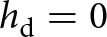 ${h_{\text{d}}} = 0$), RO is equal to the ice melt
 ${M_{\text{i}}}$, which is calculated as:
 \begin{equation}{M_{\text{i}}} = {\text{max}}\left( {0,\frac{{{Q_{{{\text{M}}_{\text{i}}}}}{{\Delta }}t}}{{{\rho _{\text{w}}}{L_{\text{m}}}}}} \right),\end{equation}
where  ${\rho _{\text{w}}}$ is the density of water,
 ${L_{\text{m}}}$ the latent heat of fusion,
 ${Q_{{{\text{M}}_{\text{i}}}}}$ the energy available for ice melt and
 ${{\Delta }}t$ the model time step. The parameters
 ${c_0}$ and
 ${c_1}$ in the energy-balance equation (Eqn (2)) are used for tuning the clean ice mass-balance model (see Section 2.2.5), while all other parameters are taken from the models of Verhaegen and others (Reference Verhaegen, Huybrechts, Rybak and Popovnin2020, Reference Verhaegen, Rybak, Popovnin and Huybrechts2024).
2.2.3.3. RO from debris-covered ice
For debris-covered ice, we use the simplified formulation of the SEB discussed in Section 2.2.2 (Eqn (3)), where the temperature-dependent fluxes  ${Q_{\Delta T}}$ have been parameterized. The iterative numerical Newton–Raphson method is then used to calculate surface temperatures from the SEB equation, which are used as an upper boundary condition for the vertical heat-transfer model. The air temperature is used as a first guess for the initial time step of the balance year and for the first time step after complete snow cover disappearance. In those cases, a simple linear vertical temperature gradient within the debris is assumed. For all other time steps, the initial guess for the surface temperature is defined as the surface temperature from the previous time step, while the change in the internal energy within the debris pack is then defined by the thermodynamic heat equation. For simplicity, our model will only incorporate the heat-conduction term and thus discards any other nonconductive processes that may contribute to heat transfer from the surface towards the ice (Fig. 3):
 \begin{equation}{\rho _{\text{d}}}{c_{\text{d}}}\frac{{\partial {T_{\text{d}}}}}{{\partial t}} = \frac{\partial }{{\partial z}}\left( {{k_{\text{d}}}\frac{{\partial {T_{\text{d}}}}}{{\partial z}}} \right)\end{equation}
with ρ is the density (kg m−3) and c the heat capacity (J kg−1 K−1) and where  $\Delta z$ is represented by a fixed number of
 ${n_{\text{d}}}$ = 10 layers (i.e.
 $\Delta z$ =
 ${h_{\text{d}}}/{n_{\text{d}}}$). The subscript ‘d’ refers to values that are applicable to the debris pack and can be thought of as a combination of the thermal properties of the rock (subscript ‘r’) and the contents of the pore spaces (subscript ‘a’), i.e.
 ${k_d} \approx {k_r}\left( {1 - {\phi _d}} \right) + {k_a}{\phi _d}$ and
 ${\rho _d}{c_d} \approx {\rho _r}{c_r}\left( {1 - {\phi _d}} \right) + {\rho _a}{c_a}{\phi _d}$, with
 ${\phi _{\text{d}}}$ the debris cover porosity. The pore spaces can be filled with air, water or ice, and the value of the debris cover porosity can vary with depth. In our model, however, we parameterize all these processes in a single depth-independent value for
 ${\rho _{\text{d}}}{c_{\text{d}}}$ and
 ${k_{\text{d}}}$, but we perform some model sensitivity experiments to evaluate how including a changing value for
 ${\phi _d}$ affects the model outcome.
To solve for the internal debris temperatures  ${T_{\text{d}}}$, we use a numerical Crank–Nicholson scheme (Reid and Brock, Reference Reid and Brock2010; Rounce and others, Reference Rounce, King, McCarthy, Shean and Salerno2018). In essence, this equation propagates the surface perturbation from the SEB equation downward as a damped and delayed thermal wave, resulting in nonlinear vertical temperature profiles. We furthermore assume that the ice is at its melting point at the ice–debris interface, maintaining a constant temperature of 0°C. The sub-debris ice melt
 ${M_{\text{d}}}$ is calculated using the downward conductive flux at the vertical ice–debris interface
 $Q_{\text{C}}^ \downarrow $, which itself depends on the temperature gradient (
 $\partial {T_{\text{d}}}$/
 $\partial z$) and the effective thermal conductivity (
 ${k_{\text{d}}}$) at the base of the debris layer (Reid and Brock, Reference Reid and Brock2010; Verhaegen and others, Reference Verhaegen, Rybak, Popovnin and Huybrechts2024):
 \begin{equation}{Q_{{{\text{M}}_{\text{d}}}}} = Q_{\text{C}}^ \downarrow = {\left( {{k_{\text{d}}}\frac{{\partial {T_{\text{d}}}}}{{\partial z}}} \right)_{\text{b}}},\end{equation}
where subscript ‘b’ implies the base of the debris layer. The sub-debris melt rate is then eventually calculated as (with  ${Q_{{{\text{M}}_{\text{d}}}}}$ the energy available for sub-debris melt):
 \begin{equation}{M_{\text{d}}} = {\text{max}}\left( {0,\frac{{{Q_{{{\text{M}}_{\text{d}}}}}{{\Delta }}t}}{{{\rho _{\text{w}}}{L_{\text{m}}}}}} \right)\end{equation}
and the eventual RO is similar to that of the clean ice mass-balance model:
 \begin{equation}RO = \left\{ \begin{array}{*{20}{c}}
{{W_s} if {h_s} \gt 0 } \\
{{M_d} if {h_s} = 0 \& {h_d} \gt 0 }
\end{array}\right. \end{equation}
The parameters  ${d_0}$,
 ${d_1}$ and
 ${k_{\text{d}}}$ in the energy-balance equation (Eqn (3)) were used for tuning the debris-covered ice mass-balance model (see Section 2.2.5). Note that we assume fully debris-covered pixels (i.e.
 ${A_{\text{d}}}$/
 $A$ = 1) for all debris thicknesses in the model unless indicated otherwise (see, e.g., Appendix A).
With  ${M_i}$ and
 ${M_d}$ known, the Østrem curve can be constructed by calculating relative melt modification factors
 ${f_{\text{d}}}$ =
 ${M_d}$/
 ${M_i}$ and plot them with respect to the corresponding debris thickness
 ${h_{\text{d}}}$. Within the Østrem curve, we then also define some notable points to quantify its shape (Popovnin and Rozova, Reference Popovnin and Rozova2002; Kirkbride and Dugmore, Reference Kirkbride and Dugmore2003; Verhaegen and others, Reference Verhaegen, Rybak, Popovnin and Huybrechts2024). These are the effective debris thicknesses (i.e. the debris thickness at which relative melt is maximally enhanced), the critical debris thicknesses (i.e. the debris thickness at which relative melt is equal to that of clean ice) and the characteristic debris thicknesses (i.e. the debris thickness at which relative melt is a fraction
 ${e^{ - 1}}$ or ∼37% of that of clean ice).
2.2.4. Model configuration and experiment design
The primary model calibration uses the Oerlemans-type surface energy balance (SEB) approach, coupled to a one-dimensional heat-conduction (HC) model that includes the temporal internal heat storage (IHS) term within the debris pack, as discussed above. Afterwards, we conduct some sensitivity experiments by varying key parameters in the model. However, in addition to this, we also perform a series of experiments with different levels of model complexity to evaluate the robustness of our sub-debris melt model approach (Table 2). Hence, we verify the results against two alternative model configurations. First, we compare the simplified SEB parameterization with a sophisticated full energy-balance model, similar to the complexity of the Verhaegen et al. (Reference Verhaegen, Rybak, Popovnin and Huybrechts2024) model. For this experiment, summer season incoming shortwave radiation ( ${S_ \downarrow }\tau $), near-surface wind speed (
 $u$), surface pressure (
 $p$), sky emissivity (
 ${\varepsilon _{\text{a}}}$) and relative air humidity (
 ${\text{R}}{{\text{H}}_{\text{a}}}$) for the 2009–25 period were obtained from ERA5-Land (Muñoz-Sabater and others, Reference Muñoz-Sabater2021) for the grid cell closest to Djankuat Glacier. These were subsequently bias-corrected using the 2009 AWS observations, following the methodology of Verhaegen and others (Reference Verhaegen, Rybak, Popovnin and Huybrechts2024). Second, we perform an experiment that excludes the temporal IHS term within the debris, thereby assuming only linear vertical temperature gradients within the debris layer. These additional experiments should provide insight into the sensitivity of the modelled sub-debris melt to the degree of physical complexity included in the debris energy-balance and heat-conduction formulation and help assess the robustness of the simplified SEB approach.
Main model configurations with varying degrees of complexity in this study. The abbreviations ‘SEB’ and ‘IHS’ stand for ‘surface energy balance’ and ‘internal heat storage’ respectively. See main text for the meaning of the symbols.

Table 2 Long description
Three model configurations for debris-covered glacier melt are compared by their surface energy balance approach, internal heat storage treatment, required atmospheric forcing, and debris input variables. The simplest option uses a parameterized surface energy balance and a simplified heat storage assumption based on linear vertical temperature gradients, forced only by air temperature, precipitation, and incoming shortwave radiation, and it needs a small set of debris properties including albedo and thermal conductivity. The main study configuration keeps the parameterized surface energy balance but adds full internal heat storage within the debris, using the same limited atmospheric forcing while requiring additional debris properties such as density and heat capacity. The most complex option computes the full debris surface energy balance and full internal heat storage, optionally allowing a vertical porosity gradient, and it requires the broadest atmospheric forcing set, adding wind, air emissivity, humidity, and air pressure to the basic inputs. It also expands debris inputs to include surface emissivity, an exchange coefficient, a surface moisture or humidity-related term, and the debris cover porosity. Overall, complexity increases from by adding more physical processes and therefore more forcing data and debris parameters. Variable names are listed as categories of inputs rather than defining measurement units or data sources, so comparability depends on consistent parameter definitions across implementations.
›In Appendix A, we further explore a potential and optional model extension in which the relative melt enhancement for thin/patchy debris is included in the model by parameterizing debris cover patchiness.
2.2.5. Model calibration
(a) Parameter values and input data
The Digital Elevation Model (DEM) from Morozova and Rybak (Reference Morozova and Rybak2017) is used to calculate the insolation based on the local slope and surface aspect using basic astronomical formulas, as well as to incorporate the effects of topographic shadow and self-shading (Verhaegen and others, Reference Verhaegen, Rybak, Popovnin and Huybrechts2024). We also use the DEM to spatialize the air temperature and precipitation fields, using elevation-dependent gradients (Verhaegen and others, Reference Verhaegen, Huybrechts, Rybak and Popovnin2020). For the atmospheric transmissivity and debris surface albedo, an AWS-derived value of 0.58 and 0.10 is assigned, respectively.
For the volumetric heat capacity  ${\rho _{\text{d}}}{c_{\text{d}}}$ in Eqn (7), values are taken over from Bozhinskiy and others (Reference Bozhinskiy, Krass and Popovnin1986) for the Djankuat Glacier. However, in other instances, standard values can be used depending on the rock lithology. For the gneiss/granite-type material that is found on the Djankuat Glacier, for example, typical values for the rock density and specific heat capacity are 2650 kg m−3 and 800 J kg−1 °C−1, respectively (Robertson, Reference Robertson1988). A value of 0.3 is also often assumed to be a good representative for the overall porosity of a debris layer (Nicholson and Benn, Reference Nicholson and Benn2013; Fontrodona-Bach and others, Reference Fontrodona-Bach2025). For our model, this implies an effective volumetric heat capacity of
 $1.5 \times {10^6}$ J m−3 °C−1.
(b) Snow and clean ice model
Model calibration of the multiyear energy/mass-balance model over the 2009–25 period starts with the tuning of the snow and clean ice mass-balance model. For that, we calibrate the parameters  ${c_0}$ and
 ${c_1}$ in Eqn (2) until the root-mean-square error (RMSE) between the observed and modelled local annual SMBs from the stake measurements in the clean ice area is minimized (Fig. 4):
 \begin{equation}{\text{RMS}}{{\text{E}}_{\text{M}}} = \sqrt {\frac{1}{{{n_{\text{M}}}}}\sum\limits_{i = 1}^{{n_{\text{M}}}} {{\left( {{b_{{\text{s}},{\text{obs}}}} - {b_{{\text{s}},{\text{mod}}}}} \right)}^2}} ,\end{equation}
where  ${n_{\text{M}}}$ is the number of local mass-balance observations in the clean ice area. We vary
 ${c_0}$ in steps of 5 W m−2 between −110 and 0 W m−2 and
 ${c_0}$ in steps of 1 W m−2 °C−1 between 2 and 25 W m−2 C−1.
Schematic visualization of the calibration procedure for the simplified surface energy-balance approach (‘simple SEB + full IHS’) in this study.

Figure 4 Long description
The flowchart illustrates the calibration process for snow/clean ice and debris-covered ice surface mass balance (SMB) models. It begins with varying parameters c_0 and c_1. The next step is to find the minimized root mean square error (RMSE) between modeled and observed b_s for snow/clean ice. Then, c_0 is used as an initial guess for d_0. The process continues by varying d_1 and k_. The next step is to find the minimized composite RMSE_CN between modeled and observed b_s and T_s for debris-covered ice. If the minimum RMSE _CN for d_1 and k_d has not yet reached its lowest value, the process loops back to adjust d_0. Finally, the process concludes with determining the final values for d_0, d_1 and k_d.
(c) Debris-covered ice model
To tune the debris-covered ice model, we follow a slightly different and more sophisticated approach. Here, we use three parameters:  ${d_0}$,
 ${d_1}$ and
 ${k_{\text{d}}}$ (Eqns (3) and (7)). However, to reduce the risk of parameter equifinality, we can restrict the parameter range of
 ${d_0}$ based on the best-fit value of
 ${c_0}$. Indeed, the value of
 ${c_0}$ (the intercept for snow/clean ice) applies for a value of
 ${T_a}$ = 0°C and
 ${d_0}$ (the intercept for debris-covered ice) for
 ${T_a}$ −
 ${T_{\text{s}}}$ = 0°C. If we assume a melting snow/ice surface (i.e. a surface temperature fixed at 0°C), the sensible heat flux is absent in both cases, and any difference in the net longwave radiation is only caused by a different surface emissivity of a snow/ice and debris surface (which, in fact, are relatively similar). For mid-latitude glaciers, the latent heat flux is furthermore of minor importance when compared to other energy fluxes most of the time. This should imply that
 ${c_0} \approx {d_0}$ and that the best-fit value for
 ${c_0}$ can thus be used as a first guess for
 ${d_0}$ in the tuning procedure for the debris-covered ice mass-balance model. This leaves two remaining parameters to be varied for a single value of
 ${d_0}$:
 ${d_1}$ and
 ${k_d}$. In a subsequent step,
 ${d_0}$ can be slightly varied to check whether this further improves the agreement between observed and modelled sub-debris melt rates and debris surface temperatures (Fig. 4).
We thus start the tuning by setting  ${d_0}$ to the calibrated value of
 ${c_0}$ and vary
 ${d_1}$ in steps of 2 W m−2 between 4 and 60 W m−2
 $^\circ $C−1 and
 ${k_d}$ in steps of 0.2 W m−1
 $^\circ $C−1 between 0.4 and 3.4 W m−1
 $^\circ $C−1. The latter is a sufficiently large interval to capture commonly reported values in the literature for
 ${k_d}$ (Rowan and others, Reference Rowan2021; Fontrodona-Bach and others, Reference Fontrodona-Bach2025). To calibrate the sub-debris melt model, we minimize a multi-objective ‘combined normalized RMSE’ (hereafter denoted
 $RMS{E_{CN}}$) using two observational datasets: (i) sub-debris melt measurements from stakes in the debris-covered area (2009–25), and (ii) debris surface temperatures measured by the AWS during the 2009 summer season:
 \begin{equation}{\text{RMS}}{{\text{E}}_{{\text{CN}}}} = \sqrt {\begin{array}{l}{w_{\text{M}}}\left[ {\frac{1}{{{n_{\text{M}}}}} \sum \limits_{i = 1}^{{n_{\text{M}}}} {{\left( {\frac{{{b_{{\text{s}},{\text{obs}}}} - {b_{{\text{s}},{\text{mod}}}}}}{{{\sigma _{{b_{{\text{s}},{\text{obs}}}}}}}}} \right)}^2}} \right]\\ + {w_T}\left[ {\frac{1}{{{n_T}}}\sum \limits_{i = 1}^{{n_T}} {{\left( {\frac{{{T_{{\text{s}},{\text{obs}}}} - {T_{{\text{s}},{\text{mod}}}}}}{{{\sigma _{{T_{{\text{s}},{\text{obs}}}}}}}}} \right)}^2}} \right]\end{array}} ,\end{equation}
where the individual terms below the square root represent  ${\text{RMS}}{{\text{E}}_{\text{M}}}$ and
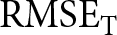 ${\text{RMS}}{{\text{E}}_{\text{T}}}$, which are the RMSE values of local mass balance and surface temperature observations, respectively, over debris-covered terrain. To make the total error dimensionless, the data are, however, normalized by the standard deviation
 $\sigma $ of the corresponding observations. Moreover, because the spread in surface temperature errors differs from that of sub-debris melt, we use weights such that both objectives affect the
 ${\text{RMS}}{{\text{E}}_{{\text{CN}}}}$ similarly:
 \begin{align}{w_M} & = \frac{{{{\overline {RMSE} }_{T\left\{ {{d_1},{k_d}} \right\}}}}}{{{{\overline {RMSE} }_{T\left\{ {{d_1},{k_d}} \right\}}} + {{\overline {RMSE} }_{M\left\{ {{d_1},{k_d}} \right\}}}}}, \nonumber\\ {w_T} & = \frac{{{{\overline {RMSE} }_{M\left\{ {{d_1},{k_d}} \right\}}}}}{{{{\overline {RMSE} }_{T\left\{ {{d_1},{k_d}} \right\}}} + {{\overline {RMSE} }_{M\left\{ {{d_1},{k_d}} \right\}}}}}\end{align}
The weights are defined by the average RMSE for the surface temperature and sub-debris melt rates over the entire parameter space of  ${d_1}$ −
 ${k_{\text{d}}}$ combinations. Although alternatives to our approach exist (e.g. tuning for the surface temperature and sub-debris melt rates separately) that may produce similar best-fit values (McCarthy, Reference McCarthy2025; Pellicciotti and others, Reference Pellicciotti2026), these steps ensure that both variables contribute equally to the composite objective, independent of differences in units or absolute magnitude of the errors. We note that
 $RMS{E_{CN}}$ represents a composite objective function rather than a classical RMSE, as it combines two datasets with different units and error structures (Deb, Reference Deb2001). In this sense, the formulation should be interpreted within a multi-objective optimization framework, where the weights determine the relative importance of sub-debris melt and surface temperatures. After each iteration of varying
 ${d_1}$ and
 ${k_d}$, we changed the offset
 ${d_0}$ with 5 W m−2 to check whether the minimum
 $RMS{E_{CN}}$ across the parameter space further decreases. The calibration procedure stops whenever a minimum for min (
 ${\text{RMS}}{{\text{E}}_{{\text{CN}}}}\left\{ {{d_1},{k_{\text{d}}}} \right\}$) as a function of
 ${d_0}$ is found (Figs 4 and 7d).
3. Model results
3.1. Parameterization of temperature-dependent fluxes from meteorological data
As mentioned before, the model of Verhaegen and others (Reference Verhaegen, Rybak, Popovnin and Huybrechts2024) was used to investigate the relationship between  ${T_a}$ and
 ${Q_{\text{L}}} + {Q_{{\text{SH}}}} + {Q_{{\text{LH}}}} + {Q_{\text{R}}}$ for snow/clean ice, and between
 ${T_{\text{a}}}$ −
 ${T_{\text{s}}}$ and
 ${Q_L} + {Q_{SH}} + {Q_{LH}} + {Q_R}$ for debris-covered ice on the Djankuat Glacier. This model consists of a detailed formulation of the 2D calibrated energy and mass balance of the clean ice and debris-covered ice areas of the entire Djankuat Glacier during the 2008/09 balance year. It used meteorological forcing from a combination of on-glacier AWSs, which were operational during the ablation season, and bias-corrected ERA5-Land data (during snow-covered conditions), which were spatialized over the entire glacier surface.
Figure 5 shows the resulting data, where the red dots display the mean flux value for each 2 $^\circ $C bin. The data for snow and clean ice follow the pattern suggested by Oerlemans (Reference Oerlemans2001): the temperature-dependent fluxes are approximately constant for air temperatures below the melting point, whereas they increase linearly for above-zero air temperatures (Fig. 5a). This effect arises because the surface temperature of melting snow and ice is fixed at 0°C, implying that once it reaches the melting point, any extra energy goes into melting instead of further surface warming. For debris-covered ice, a scaling of the temperature-dependent fluxes with air temperature alone does not produce a clear relationship (Fig. 5b). Therefore, we do not use this relationship. Instead, the fluxes scale approximately linearly with the air-surface temperature gradient, which is consistent with the formulations of longwave and turbulent heat exchange (Fig. 5; McCarthy, Reference McCarthy2025; Pellicciotti and others, Reference Pellicciotti2026). This is because the debris surface temperature itself can, in contrast to snow and ice, reach values above 0°C. When the debris surface is warmer than the air, the temperature-dependent fluxes are negative and directed away from the surface. In contrast, when the air is warmer, fluxes are positive and directed towards the surface. The corresponding best fit to the data used in Verhaegen and others (Reference Verhaegen, Rybak, Popovnin and Huybrechts2024) for the 2008/09 balance year yields values for
 ${d_0}$ = −95 W m−2 and
 ${d_1}$ = 23 W m−2
 $^\circ $C−1 (Fig. 5c). Some notable scatter remains for both clean ice and debris-covered ice, which is presumably due to varying conditions such as cloud cover, wind speed and humidity.
(a) The relationship between the air temperature and the temperature-dependent fluxes within the energy balance for a snow and clean ice surface. For a debris-covered surface (b), the relationship between the air temperature (which is not used) and (c) the air-surface temperature difference and the temperature-dependent fluxes are shown. Data are from the glacier-wide calibrated 2D energy- and mass-balance model of Verhaegen and others (Reference Verhaegen, Rybak, Popovnin and Huybrechts2024) for the 2009 summer season, which was forced by direct AWS observations and bias-corrected ERA5-Land data. Apart from the data, the averages for 2 $^\circ $C temperature bins are shown (red dots) together with the parameterization (black dashed line).

Figure 5 Long description
A scatter plot where ‘Data’ are shown as many small blue point markers, ‘2 degree celsius bin means’ are shown as larger red point markers and ‘Linear fit’ is shown as a black dashed line. The subplot A shows the relationship between the air temperature and the air temperature-dependent fluxes for snow/clean ice, subplot B does the same for a debris-covered surface. The subplot C shows the relationship between the air-surface temperature gradient and the air temperature-dependent fluxes for a debris-covered surface.
3.2. Energy- and mass-balance model calibration
Using the parameterized relationships between  ${T_{\text{a}}}$ and
 ${Q_L} + {Q_{SH}} + {Q_{LH}} + {Q_R}$ for snow/clean ice, and between
 ${T_a}$ −
 ${T_{\text{s}}}$ and
 ${Q_L} + {Q_{SH}} + {Q_{LH}} + {Q_R}$ for debris-covered ice as found above, we tuned the multiyear energy- and mass-balance model. For the snow and clean ice model, a minimum
 ${\text{RMS}}{{\text{E}}_M}$ of 0.98 m w.e. yr−1 (R 2 = 0.78) was found for values of
 ${c_0}$ = −45 W m−2 and
 ${c_1}$ = 13 W m−2
 $^\circ $C−1 (Fig. 6). These numbers closely resemble earlier values found by Verhaegen and others (Reference Verhaegen, Huybrechts, Rybak and Popovnin2020, Reference Verhaegen, Rybak, Popovnin and Huybrechts2024) for the Djankuat Glacier.
(a) The RMSE between modelled and observed local annual surface mass balances (2009–25) for snow and clean ice for different combinations of  ${c_0}$ and
 ${c_1}$, and (b) the observed and modelled local annual surface mass balances (2009–25) for the best fit of
 ${{\text{c}}_0}$ = −45 W m−2 and
 ${{\text{c}}_1}$ = 13 W m−2
 $^\circ $C−1 (
 ${\text{RMS}}{{\text{E}}_{\text{M}}}$ = 0.98 m w.e. yr−1, R 2 = 0.78).

Figure 6 Long description
A showing a contour heatmap titled, ‘RMSE modelled vs. observed local annual mass balance (snow and clean ice)’. The horizontal axis label is c_0 (W m-2) with a range negative 100 to 0. The vertical axis label is c_1 (W m-2 °C-1) with a range 0 to 25. The color scale label is RMSE (m yr -1 w.e.) with a range 1 to 5. Contour lines form bands across the plot. The lowest RMSE values appear in the plot near c_1 close to 15 and c_0 near negative 45. Higher RMSE values appear toward the upper and lower part of the plot . B shows a scatter plot titled, ‘Best fit modelled vs. observed local annual mass balance (snow and clean ice)’. The plotted points form an upward sloping band that follows the 1:1 line, with the densest cluster around modelled values near 0 to 2 and observed values near -1 to 1. Points extend to lower observed values near negative 8 at modelled values near negative 6 and to higher observed values near 2 at modelled values near 3 to 4. The two graphs relate by showing parameter combinations and their RMSE in the heatmap and the scatter plot showing modelled versus observed values for the best fit case indicated by the RMSE plot.
For the debris-covered ice part, we found a minimized combined normalized  ${\text{RMS}}{{\text{E}}_{{\text{CN}}}}$ of 0.7827 for values of
 ${d_1}$ = 40 W m−2
 $^\circ $C−1 and
 ${k_d}$ = 1.8 W m−1
 $^\circ $C−1 for the initial guess value of
 ${d_0}$ =
 ${c_0}$ = −45 W m−2. However, when further changing
 ${d_0}$, the minimum
 $RMS{E_{CN}}$ that was found for all parameter combinations of
 ${d_1}$ and
 ${k_d}$ varied slightly and reached a minimum at
 ${d_0}$ = −60 W m−2 (Fig. 7d). In that case, a minimized combined normalized
 ${\text{RMS}}{{\text{E}}_{{\text{CN}}}}$ of 0.7817 was found for values of
 ${d_1}$ = 36 W m−2
 $^\circ $C−1 and
 ${k_d}$ = 1.8 W m−1
 $^\circ $C−1. The individual RMSE values for the annual sub-debris melt and 3 hourly surface temperatures are
 ${\text{RMS}}{{\text{E}}_M}$ = 1.10 m w.e. yr−1 (R 2 = 0.46) and
 ${\text{RMS}}{{\text{E}}_T}$ = 4.38
 $^\circ $C (R 2 = 0.69) in that case. Our final best-fit values for the sub-debris melt model are thus
 ${d_0}$ = −60 W m−2,
 ${d_1}$ = 36 W m−2
 $^\circ $C−1 and
 ${k_d}$ = 1.8 W m−1
 $^\circ $C−1 (Fig. 7a–c).
(a) The observed and best-fit modelled local annual sub-debris mass balances (2009–25) for the best fit of  ${d_0}$ = −60 W m−2,
 ${d_1}$ = 36 W m−2
 $^\circ $C−1 and
 ${k_d}$ = 1.8 W m−1
 $^\circ $C−1 (
 ${\text{RMS}}{{\text{E}}_M}$ = 1.10 m w.e. yr−1, R 2 = 0.46), (b) observed and best-fit modelled 3 hourly surface temperatures for the 2009 summer season (
 ${\text{RMS}}{{\text{E}}_T}$ = 4.38
 $^\circ $C, R 2 = 0.69), (c) combined normalized
 ${\text{RMS}}{{\text{E}}_{{\text{CN}}}}$ between modelled and observed local annual surface mass balances/surface temperatures of debris-covered ice for different combinations of
 ${{\text{d}}_1}$ and
 ${k_d}$ in the case of
 ${{\text{d}}_0}$ = −60 W m−2 and (d) minimized
 ${\text{RMS}}{{\text{E}}_{{\text{CN}}}}$ across the parameter space of different values for
 ${{\text{k}}_{\text{d}}}$ and
 ${{\text{d}}_1}$ after varying
 ${{\text{d}}_0}$. The vertical dashed lines show the initial guess for
 ${{\text{d}}_0}$ =
 ${{\text{c}}_0}$ and the best-fit value of
 ${{\text{d}}_0}$ = −60 W m−2.

Figure 7 Long description
Calibration of the simplified surface energy balance and heat conduction model. (a) Comparison between modelled and observed annual sub-debris mass balance, expressed in m yr^-1 w.e., at the debris stake locations. The dashed line indicates the 1:1 agreement. (b) Comparison between modelled and observed debris surface temperatures (°C), showing good agreement across the observed temperature range. (c) Combined normalized root mean square error (RMSE_CN) as a function of the turbulent heat exchange coefficient, d_1 (5–60 W m^-2 °C^-1), and debris thermal conductivity, k_d (0.5–3.5 W m^-1 °C^-1), for a fixed intercept parameter of d_0 = -60 W m^-2. Lower RMSECN values indicate improved model performance, with the optimal parameter combinations located in the dark-blue region. (d) Minimum RMSE_CN obtained for different values of the intercept parameter d_0 (-70 to -40 W m^-2). The lowest RMSE_CN occurs at d_0 = -60 W m^-2, which was selected as the optimal parameter value for the subsequent model simulations.
The resulting best-fit Østrem curve, displaying the relative melt modification factors  ${f_{\text{d}}}$ =
 ${M_d}$/
 ${M_i}$ with respect to the corresponding debris thickness
 ${h_{\text{d}}}$, can be approximated by (Fig. 8):
 \begin{equation}{f_d} = \frac{{{M_d}}}{{{M_i}}} = {\text{max}}\left( {0.01, 0.14*h_d^{ - 0.75} - 0.05} \right)\end{equation}
The resulting Østrem curve from the best-fit parameters shown in Figure 7.

where  ${h_d}$ is expressed in metres (m).
The resulting Østrem curve from the best-fit model simulation displays the expected nonlinear decrease in relative melt rate with increasing debris thickness (Fig. 8). The curve shows that relative melt is enhanced at small debris thicknesses and then declines as the debris layer thickens, which reflects the transition from melt-enhancing to melt-suppressing conditions typical of debris-covered glaciers (Popovnin and Rozova, Reference Popovnin and Rozova2002; Kirkbride and Dugmore, Reference Kirkbride and Dugmore2003; Verhaegen and others, Reference Verhaegen, Rybak, Popovnin and Huybrechts2024). In our model, this switch occurs at a critical debris thickness  $h_{\text{d}}^{\text{c}}$ of 7 cm, which fits well with earlier values found by Popovnin and Rozova (Reference Popovnin and Rozova2002) and Verhaegen and others (Reference Verhaegen, Rybak, Popovnin and Huybrechts2024) for the Djankuat Glacier. These studies reported values of 7–8 and 9 cm, respectively, for
 $h_d^c$. Popovnin and Rozova (Reference Popovnin and Rozova2002) and Verhaegen and others (Reference Verhaegen, Rybak, Popovnin and Huybrechts2024) furthermore report (near-)negligible melt for debris thicker than ∼1-1.5 m, which is confirmed by our model as
 ${f_d}$ gradually asymptotes to (near-)zero. This further confirms the model’s ability to reproduce the characteristic melt-modification effects of supraglacial debris and adds credibility to the tuning procedure.
3.3. Model sensitivity
3.3.1. Sub-debris melt sensitivity to parameter variations
To evaluate how uncertainties in debris characteristics influence modelled sub-debris melt, we varied six key debris parameters (the effective thermal conductivity  ${k_d}$, effective volumetric heat capacity
 ${\rho _{\text{d}}}{c_{\text{d}}}$, debris albedo
 ${\alpha _{\text{d}}}$, debris cover porosity
 ${\phi _{\text{d}}}$ and the SEB tuning parameters
 ${d_0}$ and
 ${d_1}$) and examined the resulting changes in the Østrem curves (melt-modification factor versus debris thickness). To have a uniform evaluation, each parameter was varied within an interval of −50 and +50% of its original value (Fig. 9). This also ensured consistency with most reported parameter ranges within the DebDaB database (Fontrodona-Bach and others, Reference Fontrodona-Bach2025).
Sensitivity of the fitted Østrem curve to variations of debris-related key variables, including the effective thermal conductivity, effective volumetric heat capacity, debris albedo, debris cover porosity and the tuning parameters of the SEB equation  ${d_0}$ and
 ${{\text{d}}_1}$. The inset shows the corresponding effect on the characteristic debris thickness (i.e. the thickness for which sub-debris melt is a fraction
 ${e^{ - 1}}$ or ∼37% of that of clean ice). The colours represent changes from −50% (red) to +50% (blue) compared to the value used in the best-fit model.

Figure 9 Long description
Sensitivity of the melt modification factor to ±50% perturbations in the principal debris and model parameters. Each panel shows the melt modification factor as a function of debris thickness (0–2 m), with red and blue curves representing negative and positive parameter perturbations, respectively. The analysed parameters are: (a) effective thermal conductivity, k_d (W m^-1 °C^-1), (b) effective volumetric heat capacity, ρ_d*c_d (J m^-3 °C^-1), (c) debris albedo, α_d (-), (d) debris porosity, ϕ_d (-), (e) heat exchange intercept parameter, d_0 (W m^-2), and (f) heat exchange slope parameter, d_1 (W m^-2 °C^-1). Insets show the corresponding characteristic debris thickness, hc (cm), at which debris melt equals clean-ice melt, as a function of the relative parameter perturbation (Δ parameter, %). Thermal conductivity produces the largest changes in both the melt modification factor and the characteristic debris thickness, whereas the remaining parameters primarily affect the thin-debris regime, with progressively smaller sensitivities for volumetric heat capacity, albedo, porosity, d_0, and d_1.
Overall, the sensitivity experiments reveal that most parameters primarily affect the Østrem curve in the thin to moderately thick debris regime. Hence, for debris thicknesses larger than ∼1.5 m, parameter sensitivity becomes increasingly negligible across all experiments and the Østrem curves converge towards a common insulating asymptote. Among all parameters, thermal conductivity  ${k_d}$ has the strongest influence. Higher
 ${k_d}$ values are modelled to support higher melt rates under the debris by enhancing conductive heat transfer towards the ice, while lower
 ${k_d}$ values suppress melt more rapidly, producing earlier transitions to insulating behaviour. Differences gradually diminish for debris thicker than ∼1.5 m, where all values converge towards strong melt reduction. Also the debris cover porosity
 ${\phi _{\text{d}}}$ exerts a more noticeable influence by altering the effective thermal properties. Higher porosity values increase the insulation effect and reduce melt under the debris, but again the effect gradually fades for an increasingly thicker cover. The tuning parameters
 ${d_0}$ and
 ${d_1}$ affect the Østrem curve to a moderate degree and have less impact than the thermal conductivity. This is to be expected since the surface boundary condition reaches the sub-debris ice only as a dampened signal, especially for thicker debris. Changes in volumetric heat capacity
 ${\rho _{\text{d}}}{c_{\text{d}}}$ and debris albedo
 ${\alpha _{\text{d}}}$ affect the curve to a lesser degree and appear second-order or even negligible controls. Taken together, the sensitivity analysis shows that model performance is most responsive to variations in the effective thermal conductivity
 ${k_d}$ (including the effects of the porosity), moderately responsive to the temperature-dependent tuning parameters
 ${d_0}$ and
 ${d_1}$ and less responsive to surface albedo and debris pack volumetric heat capacity variations.
3.3.2. Sub-debris melt sensitivity to model complexity
As stated before, we also compare our model approach to two alternative configurations (Table 2): (i) one including the full SEB formulation (‘full SEB + full IHS’) and (ii) the other being without IHS for the heat-conduction submodule (‘simple SEB + simple IHS’). Figure 10a shows that all model configurations reproduce a similar Østrem curve, despite substantial differences in model complexity. These relatively small differences indicate that a simplified representation of the SEB (and heat-conduction process) can capture the overall magnitude and shape of the melt-debris thickness relationship with good accuracy. The error boxplots, displaying the corresponding errors (observed vs modelled values) with respect to both sub-debris melt and debris surface temperature observations for the best fit, further show that differences in sub-debris melt errors are generally small (Fig. 10b). Nevertheless, with respect to the sub-debris mass balances, we observe that the ‘full SEB + full IHS’ configuration yields the best overall results (median error: 0.102 m yr−1 w.e.) and the ‘simple SEB + simple IHS’ configuration exhibits the least accuracy (median error: 0.183 m yr−1 w.e.). The ‘simple SEB + full IHS’ approach, which is the one used in this study, produces intermediate results (median error: 0.158 m yr−1 w.e.). Differences between the degree of model complexity are more pronounced for debris surface temperatures (Fig. 10c), where the simplified configuration produces the largest errors. Again, the ‘full SEB + full IHS’ configuration yields the best results (median error: −0.389 $^\circ $C) and the ‘simple SEB + simple IHS’ configuration exhibits the largest overall errors (median error: −2.776
 $^\circ $C). The ‘simple SEB + full IHS’ approach used in this study sits in between those (median error: −1.610
 $^\circ $C).
Comparison (a) of best-fit Østrem curve reproduced by models with the full SEB (surface energy balance) and the simplified IHS (internal heat storage) for the heat-conduction model. The ‘simple SEB + full IHS’ approach corresponds to the model configuration used in this study. Subplots (b) and (c) show the boxplots of the corresponding errors (modelled values − observations) for the surface mass balances (bs) and debris surface temperatures (Ts), where the colours correspond to model configurations mentioned in the legend of subplot (a).

Figure 10 Long description
Comparison of model performance for three debris melt model configurations with increasing levels of physical complexity: simple surface energy balance (SEB) with full internal heat storage (IHS), simple SEB with simplified IHS, and full SEB with full IHS. (a) Simulated Østrem curves showing the melt modification factor as a function of debris thickness (m). All three model configurations reproduce the characteristic decrease in melt with increasing debris thickness and yield nearly identical melt modification factors over most of the debris thickness range. (b) Boxplots of the sub-debris mass balance errors, bs (m yr^-1 w.e.), for each model configuration. The full SEB with full IHS produces the smallest error spread, while the simplified configurations exhibit only slightly larger errors. (c) Boxplots of debris surface temperature errors, Ts (°C), showing comparable performance among the three model configurations, with the full SEB and full IHS providing the best overall agreement with observations. Overall, the results indicate that incorporating internal heat storage has a greater influence on model performance than employing a fully resolved surface energy balance.
4. Discussion
4.1. Model calibration and best-fit values
4.1.1. Robustness of calibrated parameter values
The calibration procedure of the sub-debris model (‘simple SEB + full IHS’) involved three unknown and tunable parameters. However, the value of  ${d_0}$ was initially constrained by the best-fit value for
 ${c_0}$. The initial guess of
 ${d_0}$ =
 ${c_0}$ already provided values close to the optimized parameter values. However, additionally decreasing
 ${d_0}$ further increased the goodness of the fit and optimized the
 $RMS{E_{CN}}$ across the different parameter combinations (Fig. 7d). Because air-surface temperature gradients (i.e. the sensible heat flux) do not impact this value and the surface emissivity of debris and snow/clean ice are relatively similar, the slight difference between the initial guess and the best-fit value of
 ${d_0}$ likely comes from differences in the latent heat fluxes between snow/clean ice (represented by
 ${c_0}$) and debris-covered ice (represented by
 ${d_0}$). Indeed, this may reflect the moderate evaporation rates from the debris surface in the rather wet climate around the Main Caucasus Ridge, leading to slightly more negative latent heat fluxes. Also, for equal wind speeds and humidity deficits, the latent heat flux is generally higher in magnitude (i.e. more negative) over rougher debris-covered terrain due to higher turbulent heat exchange coefficients (Yang et al., Reference Yang, Yao, Zhu and Wang2017; Steiner et al., Reference Steiner, Litt, Stigter, Shea, Bierkens and Immerzeel2018). This lowers the value of
 ${d_0}$ when compared to
 ${c_0}$. Therefore, for the calibration procedure in future studies, we suggest starting from a value of the initial guess of
 ${d_0}$ =
 ${c_0}$ + 5 W m−2 and subsequently decreasing the value of
 ${d_0}$. The best-fit value for
 ${d_0}$ is then the value that produces the first minimum in the curve when plotting
 ${\text{min}}\left( {{\text{RMS}}{{\text{E}}_{{\text{CN}}}}\left\{ {{k_{\text{d}}},{d_1}} \right\}} \right)$ against
 ${d_0}$, as in Fig. 7d.
The resulting modelled SMB values agree relatively well with observed ones (Figs 6 and 7). The bias was nearly eliminated by the calibration procedure for snow/clean ice (0.03 m yr−1 w.e.), while a small bias remains for sub-debris melt rates (0.20 m yr−1 w.e.). For the surface temperature, a bias of 1.1°C is still noted after minimizing the combined normalized  $RMS{E_{CN}}$. We must acknowledge that some notable scatter remains when plotting the observed and modelled sub-debris melt rates and surface temperatures (Fig. 7a and b). We attribute these to variations in variables that are not captured in our simplified model. These include wind speed, relative humidity, wetness of the debris surface and variations in atmospheric transmissivity and cloudiness. Moreover, and presumably more important for the sub-debris melt rates, spatio-temporal variations of the debris properties also play a role. Important factors that can influence these effective thermal properties are, for example, heterogeneities with respect to grain/rock sizes and their sorting (i.e. vertical porosity gradients), packing type, lithology or transient changes in moisture and ice content within the debris pack (Collier and others, Reference Collier, Nicholson, Brock, Maussion, Essery and Bush2014; Anderson and others, Reference Anderson, Armstrong, Anderson and Buri2021; Rowan and others, Reference Rowan2021; Verhaegen and others, Reference Verhaegen, Rybak, Popovnin and Huybrechts2024).
A comparison between calibrated SEB components at the AWS location during the 2008/09 balance year and those from the full SEB approach further confirms the credibility of the model (Fig. 11a). The diurnal evolution of the conductive, temperature-dependent and net shortwave flux components matches relatively well in pattern and moderately well in magnitude when different model complexities are considered. This confirms that the parameterized SEB formulation, despite its reduced complexity, can reproduce the main drivers of the SEB and the corresponding surface temperatures well. Remaining differences can be explained due to the applied simplifications in the model (e.g. the parameterization of the full SEB equation) and different model forcing datasets (i.e. bias-corrected ERA5-Land data for the full SEB implementation versus Terskol/theoretical insolation data for the simplified SEB implementation).
Comparison of (a) surface energy fluxes and (b) sub-debris melt rates at the 2009 AWS location over debris-covered terrain (hd = 65 cm) during the snow-free period for different levels of model complexity. In (a), markers represent the net shortwave radiation ( ${Q_{\text{S}}}$), the air-temperature-dependent fluxes (
 ${Q_{\Delta T}}$) and the surface conductive heat flux (
 ${Q_{\text{C}}}$). For the ‘full SEB’ approach,
 ${{\text{Q}}_{{{\Delta T}}}}$ is calculated from the individual SEB terms. Colours indicate the degree of model complexity (green: ‘full SEB + full IHS’, red: ‘simple SEB + full IHS’ and black: ‘simple SEB + simple IHS’). Subplot (c) compares the Østrem curves from the three model configurations obtained in this study to an average curve from multiple debris-covered glaciers in the literature, and (d) shows the best-fit value of the thermal conductivity from the ‘simple SEB + full IHS’ approach within a range of reported values (Fontrodona-Bachand others, Reference Fontrodona-Bach2025).

Figure 11 Long description
Comparison of the three debris melt model configurations with observations and literature values. (a) Mean diurnal surface energy balance components at the automatic weather station (AWS) located on the debris-covered glacier. The plotted fluxes include net shortwave radiation (Q_S), atmospheric heat exchange (Q_ΔT), and conductive heat flux into the debris (Q_C) for the simple surface energy balance (SEB) with full internal heat storage (IHS), simple SEB with simplified IHS, and full SEB with full IHS. All configurations reproduce the observed diurnal cycle, although the simplified IHS configuration exhibits substantially larger conductive heat fluxes. (b) Mean diurnal sub-debris melt rates (mm 3 h^-1) predicted by the three model configurations. The simple SEB with simplified IHS produces an unrealistically strong midday melt peak, whereas both configurations including full internal heat storage yield a smoother and more physically realistic diurnal melt cycle. (c) Comparison of the simulated Østrem curves with the average relationship reported in the literature. The three model configurations closely reproduce the literature-derived decrease in melt modification factor with increasing debris thickness, with only minor deviations for very thin debris. (d) Comparison of the calibrated debris thermal conductivity, k_d (W m^-1 °C^-1), obtained in this study with published literature values. The calibrated value (red star) falls within the observed range and lies close to the upper quartile of reported thermal conductivity values, indicating consistency with previous field and modelling studies.
Although the overall magnitudes of the melt rates reproduced by all model configurations are similar (Fig. 10), the temporal pattern clearly deviates for the simplified IHS model (Fig. 11b). This model configuration exhibits a strong midday melt peak associated with the direct coupling between atmospheric forcing and melt, while the full IHS model configuration reflects the buffering effect of IHS and delayed conductive heat transfer through the debris layer.
4.1.2. Comparison to literature values
A comparison between the Østrem curve derived in this study and the average curve obtained from 21 published debris-covered glacier studies (Verhaegen and Huybrechts (Reference Verhaegen and Huybrechts2026); see Fig. 11c) reveals both similarities and notable differences. The literature indicates that effective debris thicknesses (i.e. the debris thickness at which relative melt is maximally enhanced) commonly fall within 0–0.02 m, critical debris thicknesses (i.e. the debris thickness at which relative melt is equal to that of clean ice) within 0.02–0.05 m and the characteristic debris thicknesses (i.e. the debris thickness at which relative melt is a fraction  ${e^{ - 1}}$ or ∼37% of that of clean ice) around 0.10–0.15 m. The aggregated values from the literature-derived averages (0.015, 0.041 and 0.138 m respectively) produce an Østrem-type relationship as demonstrated by the purple curve in Fig. 11c. Although the shape of the Østrem curves is similar, the average Østrem curve represents a slightly stronger insulating behaviour than the curve for the Djankuat Glacier. This indicates that the debris at Djankuat reduces ablation slightly less efficiently than is typically observed on other debris-covered glaciers. This behaviour is consistent with earlier findings from Popovnin and Rozova (Reference Popovnin and Rozova2002) and Verhaegen et al. (Reference Verhaegen, Rybak, Popovnin and Huybrechts2024). These studies already showed that Djankuat’s debris layer conducts heat relatively efficiently, which shifts the Østrem curve upward for the same debris thickness.
As elaborated in Verhaegen and others (Reference Verhaegen, Rybak, Popovnin and Huybrechts2024), this is presumably due to a combination of site-specific debris properties and climatic conditions. The debris cover on Djankuat has been noted to exhibit a defined vertical layering, with the presumed presence of a vertical gradient of the debris cover porosity. This stratification—driven by downward transport and the filling of voids by finer particles, compaction of material at depth, melt-out of unsorted glacial till from the ice beneath and stone cracking at the bottom of the debris by freeze-thaw cycles—may create depth-dependent debris properties that promote a more efficient heat transfer and might help explain the relatively high effective thermal conductivity values. In addition, the rock thermal conductivity of the granite-type lithology is already relatively high (∼2.8 W m−1 K−1), which further contributes to this effect (Bozhinskiy and others, Reference Bozhinskiy, Krass and Popovnin1986). Moreover, the heat transported by rainwater through the debris layer, which can additionally impact sub-debris melt rates in the relatively wet climate around the northern slope of the Main Caucasus Ridge, may be a supplementary factor to consider (Verhaegen and others, Reference Verhaegen, Rybak, Popovnin and Huybrechts2024). Nevertheless, we also note that a comparison of Østrem curves from different glaciers or settings may not be the most appropriate strategy, due to potential sampling biases in the literature and/or the high spatio-temporal variability of the properties shaping the Østrem curve. In principle, an Østrem curve can be defined for any spatial or temporal scale. For example, the variability in climatic conditions and debris properties can be substantial on large debris-covered glaciers, such that these may require multiple Østrem curves to adequately represent melt behaviour.
Next, the calibration of the simplified energy-balance and heat-transfer model yields parameter values that are broadly consistent with expectations for debris-covered glaciers. The optimized effective thermal conductivity of 1.8 W m−1 °C−1 falls within the general interval reported for supraglacial debris in mountain glacier environments (see Fig. 11d), although our best-fit estimate falls within the high end of that range (Nicholson and Benn, Reference Nicholson and Benn2006; Reid and Brock, Reference Reid and Brock2010; Collier and others, Reference Collier, Nicholson, Brock, Maussion, Essery and Bush2014; Rowan and others, Reference Rowan2021; Fontrodona-Bach and others, Reference Fontrodona-Bach2025). The best-fit value also agrees well with earlier values derived for the Djankuat Glacier from experiments (Bozhinskiy and others, Reference Bozhinskiy, Krass and Popovnin1986; Popovnin and Rozova, Reference Popovnin and Rozova2002) and detailed 2D energy/mass-balance modelling (Verhaegen and others, Reference Verhaegen, Rybak, Popovnin and Huybrechts2024). These previous estimates for the granite/gneiss-type rocks on Djankuat lie within the 1.6–2 W m−1 °C−1 range, depending on the value of the porosity (and the presence of moisture) with depth. Likewise, calibrated values for the temperature-dependent fluxes are within physically plausible bounds and reflect the relatively strong atmospheric coupling observed at Djankuat Glacier, where thick debris layers frequently exceed air temperatures by >15°C on clear summer days.
4.2. Model sensitivity
Within this model framework, variations in  ${k_d}$ impact the sub-debris melt rates to the strongest degree, thereby significantly shifting the Østrem curve upward or downward for the same debris thickness (Fig. 9). Higher
 ${k_d}$ values facilitate the transmission of surface heat to the ice–debris interface, whereas lower
 ${k_d}$ values promote stronger melt suppression. The tuning parameters
 ${d_0}$ and
 ${d_1}$ act on the temperature-dependent flux components of the debris SEB and influence the shape and slope of the Østrem curve. Decreasing
 ${d_0}$ (i.e. making the offset for the SEB more negative) decreases the average temperature of the debris layer. This, in turn, decreases the sub-debris melt rates and shifts the Østrem curve slightly downward for a given debris thickness. This can be thought of as, for example, a wet and rough debris surface with efficient evaporation and corresponding surface cooling. Changes of the
 ${d_1}$ parameter (i.e. changing the slope of the
 ${T_a}$ −
 ${T_{\text{s}}}$ vs
 ${Q_{{{\Delta }}T}}$ curve) affect the sub-debris melt rates in a slightly more complex way. Variations in
 ${d_1}$ affect the slope of the relationship between
 ${Q_{\Delta T}}$ and
 ${T_a}$ −
 ${T_s}$. In the moderate to thick debris regime, where generally
 ${T_a}$ −
 ${T_s}$ ≪ 0 and
 ${Q_{\Delta T}}$ < 0, increases in
 ${d_1}$ decrease the average temperatures, as well as the sub-debris melt rates, in a nonlinear way. This shifts the Østrem curve downward. In the thin debris regime, where
 ${T_a}$ −
 ${T_s}$
 $ \geqslant $ 0 and
 ${Q_{\Delta T}}$
 $ \geqslant $ 0 overall, the opposite occurs, and the Østrem curve shifts upward when
 ${d_1}$ increases. This effect arises because an increasing slope of the
 ${T_a}$ −
 ${T_s}$ vs
 ${Q_{{{\Delta }}T}}$ curve amplifies the magnitude of both positive (for thin debris) and negative (for moderate to thick debris) values of
 ${Q_{{{\Delta }}T}}$ and therefore changes the curvature of the Østrem curve. Together, these processes explain why perturbations in
 ${k_d}, {d_0}$ and
 ${d_1}$ produce Østrem curves that differ not only in overall melt magnitude but also in curvature. This combined sensitivity suggests that variations in vertical debris heat transfer and temperature-dependent surface fluxes represent the largest sources of structural sensitivity in our simplified debris melt model (Fig. 9).
At first glance, the relatively weak sensitivity to debris albedo and volumetric heat capacity may appear surprising (Fig. 9). However, although an applied ±50% variation would imply a significant change in terms of albedo, this translates into a much smaller relative change in terms of net shortwave radiation. Together with the dampening of the surface signal with depth within the debris layer, this explains the comparatively minor influence of albedo on the modelled melt response. Moreover, the volumetric heat capacity mainly affects the temporal lag and variability of melt energy reaching the ice, but its impact on the overall sub-debris melt magnitude is generally limited over longer (>24 hours) timescales. With respect to the sensitivity experiments in general, it is also important to acknowledge that for some variables, their natural variability may be less/more than the ±50% change that was applied in this study.
4.3. Comparison of simplified and more sophisticated approaches
The relatively limited differences between energy fluxes and Østrem curves obtained with both the simplified and full SEB approaches (Figs 10a and 11a) indicate that a reduced-complexity parameterization provides a suitable compromise between physical realism and model complexity with regard to the SEB over debris. Fully resolving the SEB requires additional meteorological input data and (hard-to-constrain) model parameters, which are frequently unavailable in glacierized mountain regions. Although reanalysis products such as ERA5-Land can partly address these limitations, they still require bias correction and may introduce additional uncertainties in complex terrain (for example, with respect to large-scale synoptic-scale wind patterns versus small-scale katabatic/anabatic glacier winds). The results presented here suggest that, at least for reproducing annual-scale surface energy fluxes and Østrem curves, much of the essential behaviour can already be captured using a simplified SEB formulation.
Furthermore, the limited sensitivity of the volumetric heat capacity on the eventual Østrem curves would suggest that an even more simplified representation related to the heat-conduction process (i.e. using linear vertical temperature profiles within the debris, such as done in, e.g., Nicholson and Benn, Reference Nicholson and Benn2006) may be appropriate when data are considered over the entire balance year (Fig. 10a). This can then be justified by (i) the fact that such temperature profiles are approximately linear when averaged over longer temporal intervals (Nicholson and Benn, Reference Nicholson and Benn2006; Reid and Brock, Reference Reid and Brock2010) and (ii) the limited model sensitivity to the volumetric heat capacity (Fig. 9). Nevertheless, the comparison between the different model configurations also revealed substantial differences in the simulated temporal melt patterns. In particular, the ‘simple IHS’ configuration produced a deviating direct coupling between atmospheric forcing and sub-debris melt, resulting in pronounced midday melt peaks (Fig. 11b). The assumption of a linear temperature gradient may therefore limit model accuracy, especially for thicker debris layers and shorter time intervals (Pellicciotti and others, 2026). This indicates that simplified heat-conduction approaches may still inadequately represent the short-term variability of melt, even when annual melt totals remain relatively well reproduced. In that sense, a comprehensive representation of the within-debris heat-conduction and internal heat storage process seems to be more important than fully resolving the SEB for accurately reproducing sub-debris melt rates.
4.4. Transferability and considerations for application to other glaciers
4.4.1. Data requirements for transferability
The calibration strategy presented here can be readily transferred to the glacier-wide scale, whether or not coupled to a ‘patchy debris’ submodule for the thin debris regime (see Appendices A and B). The procedure can also be applied to other debris-covered glaciers, provided that a robust set of observations is available and certain considerations are taken into account. Most importantly, (i) SMB measurements (whether or not from stakes) on both clean ice and debris-covered areas are required, ideally spanning a sufficiently broad range of debris thicknesses to capture the full shape of the Østrem curve, and (ii) surface temperatures over debris-covered terrain (whether or not from an AWS) are necessary to constrain the temperature-dependent flux parameterization. Additionally, subsurface temperature measurements within the debris layer can also be used within the calibration procedure, provided (i) that IHS within the debris pack is accounted for in the model, and (ii) modelled and measured subsurface temperatures are compared at the same depth (which may require interpolation). Such datasets exist for several well-studied debris-covered glaciers worldwide, including the Kennicott Glacier, Miage Glacier, Piramide Glacier, Tasman Glacier, Lirung Glacier, Tapado Glacier, Suldenferner Glacier, Changri Nup Glacier and Arolla Glacier, where long-term monitoring programmes provide both sub-debris melt measurements and AWS-derived surface temperature records suited for model calibration (Brock and others, Reference Brock, Mihalcea, Kirkbride, Diolaiuti, Cutler and Smiraglia2010; Vincent and others, Reference Vincent2016; Anderson and others, Reference Anderson, Armstrong, Anderson and Buri2021; Steiner and others, Reference Steiner, Kraaijenbrink and Immerzeel2021; Fontrodona-Bach and others, Reference Fontrodona-Bach2025; Pellicciotti and others, Reference Pellicciotti2026). Nevertheless, these observational requirements could increasingly be supplemented or (partially) replaced by newly emerging remote sensing approaches. For example, SMB estimates may be derived geodetically from remotely sensed surface elevation change and surface velocity observations through application of the continuity equation for ice thickness change (Van Tricht and others, Reference Van Tricht, Huybrechts, Van Breedam, Vanhulle, Van Oost and Zekollari2021; Bhushan and others, Reference Bhushan, Shean, Hu, Guillet and Rounce2024; Kraaijenbrink and Immerzeel, Reference Kraaijenbrink and Immerzeel2025), combined with distributed debris thickness estimates (Rounce and others, Reference Rounce, Hock, McNabb, Millan, Sommer and Braun2021; Bisset and others, Reference Bisset2023; Gök and others, Reference Gök, Scherler and Anderson2023). Likewise, debris surface temperatures may also be obtained from UAV-based or satellite-derived thermal observations (Groos and others, Reference Groos, Mayer, Smiraglia, Diolaiuti and Lambrecht2017; Kraaijenbrink and others, Reference Kraaijenbrink2018). However, such remote sensing-derived mass balance and temperature values typically have greater uncertainties, which could impact the accuracy of the derived parameters. Moreover, if no direct clean ice melt data are available, first-guesses for  ${d_0}$ to be used in the calibration procedure of debris-covered glaciers can also be obtained from best-fit
 ${c_0}$ estimates of nearby glaciers from Giesen and Oerlemans (Reference Giesen and Oerlemans2012) or Huss and Hock (Reference Huss and Hock2015).
4.4.2. Limitations and applicability
While the calibration procedure is transferable, several considerations must be acknowledged when applying it to other debris-covered glaciers.
First, the representativeness of the available observations is critical: many debris-covered glaciers exhibit strong spatial heterogeneity in debris thickness, grain size, moisture content and aerodynamic conditions, all of which influence the debris-atmosphere energy exchange and/or efficiency of vertical heat conduction (Miles and others, Reference Miles, Steiner, Buri, Immerzeel and Pelliciotti2022; Verhaegen and others, Reference Verhaegen, Rybak, Popovnin and Huybrechts2024; Fontrodona-Bach and others, Reference Fontrodona-Bach2025). Such heterogeneity may not be captured by a sparse observational network. Consequently, model quality depends not only on the number of observations but also on how well these measurements sample the variability of the debris-covered glacier surface. Although our model uses effective debris thermal properties that are assumed constant in space and time, the inherent presence of spatially and temporally varying debris properties introduces an additional structural uncertainty. This is particularly true for debris ice/moisture content, the packing type or the grain size sorting (i.e. vertical porosity gradients), which could additionally influence the effective thermal conductivity and volumetric heat capacity.
Second, the temperature-dependent flux parameterization assumes that the dominant energy pathways can be adequately constrained from debris surface temperatures. The model quality might, therefore, also depend on how well the climate conditions have been captured. Moreover, this assumption may furthermore require verification in environments with contrasting climatic regimes. Giesen and Oerlemans (Reference Giesen and Oerlemans2012) already showed that in some cases, for example for tropical glaciers, humidity indices (or a combination of temperature and humidity indices) may be a better predictor of the magnitude of the temperature-dependent fluxes than temperature alone. For glaciers in monsoon-influenced or highly maritime climates, where seasonal precipitation regimes can vary considerably and debris moisture content may fluctuate substantially, the addition of a meltwater percolation scheme or the use of seasonally varying tuning parameters can additionally supplement the model (Fugger and others, Reference Fugger2022; Collier and others, Reference Collier, Nicholson, Brock, Maussion, Essery and Bush2014; Giese and others, Reference Giese, Boone, Wagnon and Hawley2020). Nonconductive processes, such as within-debris convection and phase changes (e.g. evaporative cooling), are furthermore not included in the model but may be important within certain environmental settings (Petersen and others, Reference Petersen, Hock, Fochesatto and Anderson2022).
A third limitation of the present formulation is its omission of supraglacial ice cliffs and ponds/lakes, which are increasingly recognized as important ablation hotspots on many debris-covered glaciers. Numerous studies have shown that cliffs and ponds can collectively account for a significant part of the ablation on thick debris-covered glaciers, despite occupying only a small fraction of the debris-covered area (Buri and others, Reference Buri, Miles, Steiner, Ragettli and Pellicciotti2021; Ferguson and Vieli, Reference Ferguson and Vieli2021; Rowan and others, Reference Rowan2021; Kneib and others, Reference Kneib2023). For the Djankuat Glacier, the impact of this omission is likely minimal: field observations indicate that supraglacial cliffs and ponds are very sparse or nearly absent and, therefore, do not constitute a significant component of the glacier’s overall melt budget. However, when transferring the approach to other debris-covered glaciers, the neglect of these features may lead to an underestimation of total ablation and a misrepresentation of the spatial melt pattern. Nonetheless, our intention is to keep the model as simple as possible, thereby addressing the trade-off between computational efficiency, model complexity and physical realism.
5. Conclusion
In this study, we developed and calibrated a physically based yet computationally efficient parameterization and calibration procedure to simulate melt beneath supraglacial debris, using stake-derived mass-balance observations and debris surface temperature measurements from the Djankuat Glacier in the Caucasus region. By parameterizing the SEB with an Oerlemans-type formulation and inserting the resulting surface temperatures as an upper boundary condition into a vertical heat-conduction model that accounts for within-debris heat storage, the model accurately reproduces observed surface temperature patterns and energy fluxes, as well as the characteristic Østrem curve. In doing so, several difficult-to-constrain inputs have been replaced by simplified and tunable variables and parameters, thereby balancing physical realism, model performance and model complexity. An optional model extension for the relative melt enhancement of thin debris is furthermore introduced in Appendix A.
Results from our approach were compared to model configurations that (i) exhibit a full energy-balance approach and (ii) do not include IHS within the debris pack (and hence assume linear vertical debris temperature gradients). The following main conclusions were drawn:
• Our modelling approach (‘simple SEB + full IHS’) produced a good agreement with observations. When comparing our results to different degrees of model complexity, our results outperform the outcome of the simplest model configuration (‘simple SEB + simple IHS’), but the fully resolved configuration (‘full SEB + full IHS’), however, still yields the best overall performance.
• Overall differences between the model configurations remain, however, relatively small. The close agreement between the parameterized and fully resolved SEB configurations indicates that simplified SEB approaches can reproduce the main patterns in surface energy fluxes and debris surface temperatures with good accuracy.
• Although all model configurations reproduced the Østrem curve and annual sub-debris melt reasonably well, the overly simplified heat-conduction approach (‘simple SEB + simple IHS’) produced deviating temporal melt patterns. Together with the strong modelled sensitivity to effective thermal conductivity, this emphasizes the importance of accurately representing the within-debris heat-conduction and heat storage process when modelling sub-debris melt.
• Finally, the adopted model physics, in which sub-debris melt is governed solely by conductive heat transfer through the debris layer, are not fully valid within the thin debris regime. In such conditions, additional parameterizations (e.g. accounting for a patchy debris cover) are required to realistically reproduce the melt enhancement observed for thin debris and dirty ice (see Appendix A).
The model’s efficiency and the relatively limited amount of inputs compared to more sophisticated models make the framework also suitable for incorporation into larger-scale debris-covered glacier evolution models. Nevertheless, applying the model elsewhere may require careful consideration of local debris thermal properties, observational constraints and unresolved processes such as heterogeneities related to spatially and temporally varying debris properties. These may include, for example, the presence of air, water and ice within the debris pack pore spaces and the occurrence of supraglacial cliffs and ponds. Future work should therefore focus on improving distributed debris thickness and properties datasets, incorporating debris heterogeneity and evaluating simulated sub-debris melt within different environmental settings and/or larger-scale glacier modelling frameworks. This will be essential to further enhance the ability to represent melt beneath supraglacial debris, especially when projecting the future behaviour of debris-covered glaciers under continued climate change on local, regional and global scales.
Data availability statement
The model code was uploaded in a GitHub repository (https://github.com/yoniv1/Simplified-sub-debris-melt-model) and can also be accessed through Zenodo (10.5281/zenodo.21668412).
Acknowledgements
Y.V. was supported by the Copernicus Climate Change Service (C3S) implemented by the European Centre for Medium-Range Weather Forecasts on behalf of the European Commission under the service contract ECMWF/Copernicus/2021/C3S2_520_CNR. The investigation in this paper has been based on the results of the fieldwork carried out by V.P. and A.G. and their team, under the State Assignment of the Lomonosov Moscow State University (126042220304-6): ‘Terrestrial and ground glaciations under the conditions of present climate change and technogenic impact’.
Author contributions
Y.V. constructed and calibrated the numerical model, performed the numerical simulations and wrote most of the manuscript. P.H. provided supervision, guidance in interpreting the results and improved the manuscript throughout the entire process. A.G. and V.P. contributed by performing glacier fieldwork, providing numerous datasets and improving the manuscript with their knowledge and years of experience concerning the Djankuat Glacier
Appendices
Appendix A – A potential model extension to include the relative melt enhancement for thin debris
Our model does not allow for the quantification of a relative enhancement for thin debris of a few centimetres thick, which is nevertheless often assumed to be present in a typical Østrem curve (Østrem, Reference Østrem1959; Bozhinskiy and others, Reference Bozhinskiy, Krass and Popovnin1986; Reid and Brock, Reference Reid and Brock2010; Rounce and others, Reference Rounce, King, McCarthy, Shean and Salerno2018). The treatment of such relative melt enhancement for thin debris, however, deserves special attention. Since the conductive heat flux through the debris layer is dependent on the debris thickness in the denominator, the sub-debris melt model as described in Sections 2.2.2 and 2.2.3 produces unrealistically high sub-debris melt rates for very small debris thicknesses. In the limit  ${h_d}$ → 0, the conductive heat flux term theoretically becomes infinite, which leads to unphysical behaviour because the melt rates should generally approach those of clean ice again when
 ${h_d}$ → 0. Despite observational and theoretical evidence that thin debris can enhance melt (e.g. in regions of ‘dirty ice’ with a lower surface albedo (Fyffe and others, Reference Fyffe, Woodget, Kirkbride, Deline, Westoby and Brock2020)), most numerical glacier models have either inserted a minimum debris thickness threshold or have neglected this melt-enhancing effect and therefore omit the rising limb of the Østrem curve (Rowan and others, Reference Rowan, Egholm, Quincey and Glasser2015; Anderson and Anderson, Reference Anderson and Anderson2016; Verhaegen and others, Reference Verhaegen, Huybrechts, Rybak and Popovnin2020; Ferguson and Vieli, Reference Ferguson and Vieli2021). This omission is often justified by (i) the scarcity and inconclusiveness of observations in thin debris regions (e.g. Rowan and others, Reference Rowan, Egholm, Quincey and Glasser2015), (ii) difficulties related to accurately measuring the thickness of (patchy) debris layers of only a few cm thick or (iii) simply for pragmatic reasons (Anderson and Anderson, Reference Anderson and Anderson2016). This is defensible given that the dominant role of debris is generally to insulate the ice. Also, our model lacks observations of thinly debris-covered regions, mainly due to the above-mentioned reasons. The absence of reliable observations over thin debris at Djankuat, and the difficulties related to obtaining and modelling them, therefore, similarly prevents a physics-based calibration of melt enhancement for
 ${h_d}$ of a few centimetres. Only a handful of studies have tried to approximate the rising limb of the curve by either the inclusion of an evaporative heat flux at the vertical debris–ice interface (Evatt and others, Reference Evatt2015), by accounting for the patchiness of thin debris (Reid and Brock, Reference Reid and Brock2010; Verhaegen and others, Reference Verhaegen, Rybak, Popovnin and Huybrechts2024), or by empirical parameterizations (Compagno and others, Reference Compagno2022).
(a) The resulting parameterization of the fractional debris-covered area with debris thickness, and (b) integration of the resulting modelled melt enhancement into the earlier calibrated Østrem curve of the ‘simple SEB + full IHS’ approach.

Figure A1 Long description
Incorporation of the thin-debris enhancement parameterization into the Østrem curve. (a) Relationship between debris thickness (m) and the fractional debris-covered area (-) derived from the calibrated stretched exponential function. Blue points represent the input data, while the red dashed line shows the fitted function, indicating that the fractional debris-covered area rapidly approaches unity as debris thickness increases. (b) Best-fit modelled Østrem curve showing the melt modification factor, f_d (-), as a function of debris thickness. Blue points represent the calibrated model output, while the black points denote the additional melt enhancement introduced for very thin debris to reproduce the characteristic Østrem peak. The parameterization increases melt above clean-ice values for debris thinner than a few centimetres while preserving the insulating effect of thicker debris, resulting in an Østrem curve consistent with field observations and published literature.
To counteract the numerical feature of the failing sub-debris melt model and simultaneously reproduce the rising limb in the Østrem curve in this study, we follow the patchy debris approach. To derive a relationship between the fractional debris-covered area and the debris thickness on the glacier, we combined data from remote sensing with our earlier calibrated sub-debris melt model. For that, we selected the balance year with the largest number of debris-covered ablation stakes (2024/25, n = 7), for which both the SMB and debris thickness were measured. A cloud-free Landsat 8 OLI/TIRS C2 L2 thermal image of the glacier region at the end of the summer season (acquired on 24 August 2025 at 10:55 local time) was then used to estimate glacier-wide surface temperatures  ${T_s}$. For that, modelled surface temperatures from our model at the stake locations were linearly interpolated between the 09:00 and 12:00 outputs to match the Landsat acquisition time. To then obtain a spatially continuous surface temperature field consistent with the calibrated model, Landsat-derived surface temperatures were bias-corrected using a linear transformation (with a slope and intercept), fitted by minimizing the RMSE between Landsat surface temperature estimates and the calibrated surface temperatures at the debris-covered stake locations. The resulting transformation was applied to the full Landsat scene (RMSE = 3.96°C, R 2 = 0.67). Debris thickness was then estimated by fitting a Hill-type function (with three tuning parameters) between observed debris thicknesses and modelled surface temperatures at the stake locations, as also done in previous studies (see Rounce and others, Reference Rounce, Hock, McNabb, Millan, Sommer and Braun2021). Applying this relationship to the bias-corrected Landsat surface temperature field yielded a distributed debris thickness estimate over the entire glacier area. At last, the fractional debris-covered area was independently derived from cloud-free Sentinel-2 L1C surface reflectance imagery, acquired on 29 August 2025, using linear spectral unmixing. Three end members (clean ice, snow and supraglacial debris/bedrock) were defined from representative training areas, and per-pixel debris fractions were then retrieved using the spectral signature of 12 different bands contained in the remote sensing imagery. Finally, the debris thickness and fractional debris-cover maps were combined by binning the mean fractional debris-covered area in 0.01 m debris thickness intervals, resulting in a glacier-specific relationship between debris thickness and the fractional debris-covered area (Figure A1). This relationship was used to constrain the thin-debris regime of the Østrem curve, i.e. beyond the range covered by our ablation stake measurements.
Melt modification in the patchy thin-debris regime is, as such, assumed to be a mix of clean ice melt and sub-debris melt, of which the subsequent weights depend on the fractional debris-covered area. For that, we follow the approach in Reid and Brock (Reference Reid and Brock2010) and Ferguson (Reference Ferguson2022) and calculate the ‘patchiness-corrected’ melt as:
 \begin{equation}{M_{\text{d}}} = \frac{{{A_{\text{d}}}}}{A}\overline {{M_{\text{d}}}} + \left( {1 - \frac{{{A_{\text{d}}}}}{A}} \right){M_{\text{i}}},\end{equation}
where  $\overline {{M_{\text{d}}}} $ is the melt corresponding to the patch-corrected debris thickness
 $\overline {{h_{\text{d}}}} $ in the pixel:
 \begin{equation}\overline {{h_d}} = \frac{{{h_d}}}{{\left( {\frac{{{A_d}}}{A}} \right)}}, if\left( {\frac{{{A_d}}}{A}} \right) \gt 0\end{equation}
The term  $\overline {{h_d}} $ hence represents how thick debris must be within patches to produce the observed grid-mean thickness
 ${h_d}$ when debris does not fully cover the surface. Moreover,
 ${A_{\text{d}}}/A$ is the fractional debris-covered area in the pixel, which is given as (Reid and Brock, Reference Reid and Brock2010):
 \begin{equation}\frac{{{A_{\text{d}}}}}{A} = 1 - {\text{exp}}\left( { - C{h_{\text{d}}}} \right)\end{equation}
for which  $C$ is derived from a fit to the earlier obtained debris thickness vs fractional debris-covered area function. A best fit value was found for
 $C$ = 32.8 (Figure A1). In this case,
 ${A_{\text{d}}}/A$ asymptotes towards 1 around
 ${h_d}$ = 0.1 m. We then let the model run with observed stake debris thicknesses divided by 10 and excluding any debris thicknesses higher than 0.1 m. The application of the melt-enhancement parameterization results in (i) a clean ice melt value in the case of zero debris thickness (since
 ${A_{\text{d}}}/A$ = 0), (ii) a melt enhancement of ∼1.44 at
 ${h_d}$ = ∼1.5–2 cm and (iii) a largely unaffected Østrem curve for a debris thickness larger than the critical thickness
 $h_d^c$ (since
 ${A_d}/A$ quickly approaches 1) (Figure A1).
We stress that this correction is only applied to small debris layers of a few centimetres thick (i.e. generally where  ${A_d}/A$ < 1 and
 ${M_{\text{d}}}/{M_{\text{i}}}$ > 1), for which our model physics is not valid (because the conductive heat transfer becomes unrealistically large as debris thickness approaches zero, and because other processes than conduction, such as increased shortwave radiation absorption or debris patchiness, may be dominant in controlling melt rates). It does not affect the calibrated melt suppression regime of the Østrem curve (i.e. generally where
 ${A_d}/A$ = 1 and
 ${M_d}/{M_i}$ < 1). The adjustment is applied after the model calibration and is constrained by a combination of observations and physically derived estimates of the surface temperatures, debris thicknesses and the fractional debris-covered area from remote sensing. It is, therefore, not an arbitrary model extension, nor is it an internal product of our energy- and mass-balance model. Rather, it compensates for physical processes that apply to thin debris layers which cannot be represented through heat conduction alone. Because the source data for applying this model extension are generally publicly available, this approach is readily applicable to other debris-covered glaciers. This supports the broader suitability of the parameterization.
In this case, the curve can be approximated by:
 \begin{align}
f_d = \frac{M_d}{M_i}
=\begin{cases}
1 + 29.4*\,h_d, & \text{if } h_d \leq h_d^{e}, \\[4pt]
-9*\,h_d + 1.585, & \text{if } h_d \gt h_d^{e} \,\&\, h_d \leq h_d^{c}, \\[4pt]
\max\left(0.01,\;0.14*\,h_d^{-0.75} - 0.05\right),
& \text{if } h_d \gt h_d^{c}.
\end{cases}\end{align}
where  ${h_d}$ is expressed in metres (m).
The inclusion of the melt enhancement behaviour can be useful for applications in which thin debris layers may occur, such as for glacier-wide mass-balance modelling of transient, debris-covered glacier evolution. The suggested approach in our paper ensures that the model remains physically robust in the thicker debris domain for which it was calibrated, while offering an extension to capture melt enhancement effects if required by specific modelling contexts.
Simulated surface mass-balance (SMB) distribution for the 2021/22 balance year on Djankuat Glacier using the calibrated ‘simple SEB + full IHS’ model configuration together with the patchy debris cover parameterization and the measured 2022 debris thickness distribution (see inset, Popovnin and Gubanov, Reference Popovnin and Gubanov2025).

Figure A2 Long description
Spatial distribution of the simulated annual surface mass balance on Djankuat Glacier for the 2022 glacier geometry. Surface mass balance is expressed in m yr^-1 w.e., with blue colours indicating positive mass balances and red colours indicating high melt (more negative mass balances). Melt rates increase from the high-elevation accumulation area towards the low-elevation glacier tongue, reflecting the combined influence of the altitudinal temperature and precipitation gradients and the spatial distribution of supraglacial debris. The inset shows the corresponding debris thickness distribution (m), illustrating progressively thicker debris towards the glacier terminus, where debris thickness locally exceeds 1 m. The lower glacier tongue experiences the greatest annual ablation due to the strong climatic forcing at low elevations, while the insulating effect of thick debris reduces melt relative to adjacent clean-ice areas.
Appendix B – Integration in full mass-balance model and application to the glacier scale
To evaluate the distributed impact of supraglacial debris on glacier melt when including the relative melt enhancement parameterization above, the 2D SMB field over the Djankuat Glacier was simulated for the 2021/22 balance year. This corresponds to the year for which the latest glacier-wide measured debris thickness map is available (Popovnin and Gubanov, Reference Popovnin and Gubanov2025). The calibrated ‘simple SEB + full IHS model’ configuration, together with the patchy debris cover parameterization, was therefore applied glacier-wide using the distributed debris thickness field as model input. The resulting SMB distribution is shown in Figure A2. As expected, the model reproduces the characteristic enhancement of melt beneath thin debris layers, while thicker debris leads to a clear suppression of melt due to the insulating effect of the debris cover. This demonstrates the potential applicability of the model to the glacier-wide scale and within debris-covered glacier evolution frameworks.
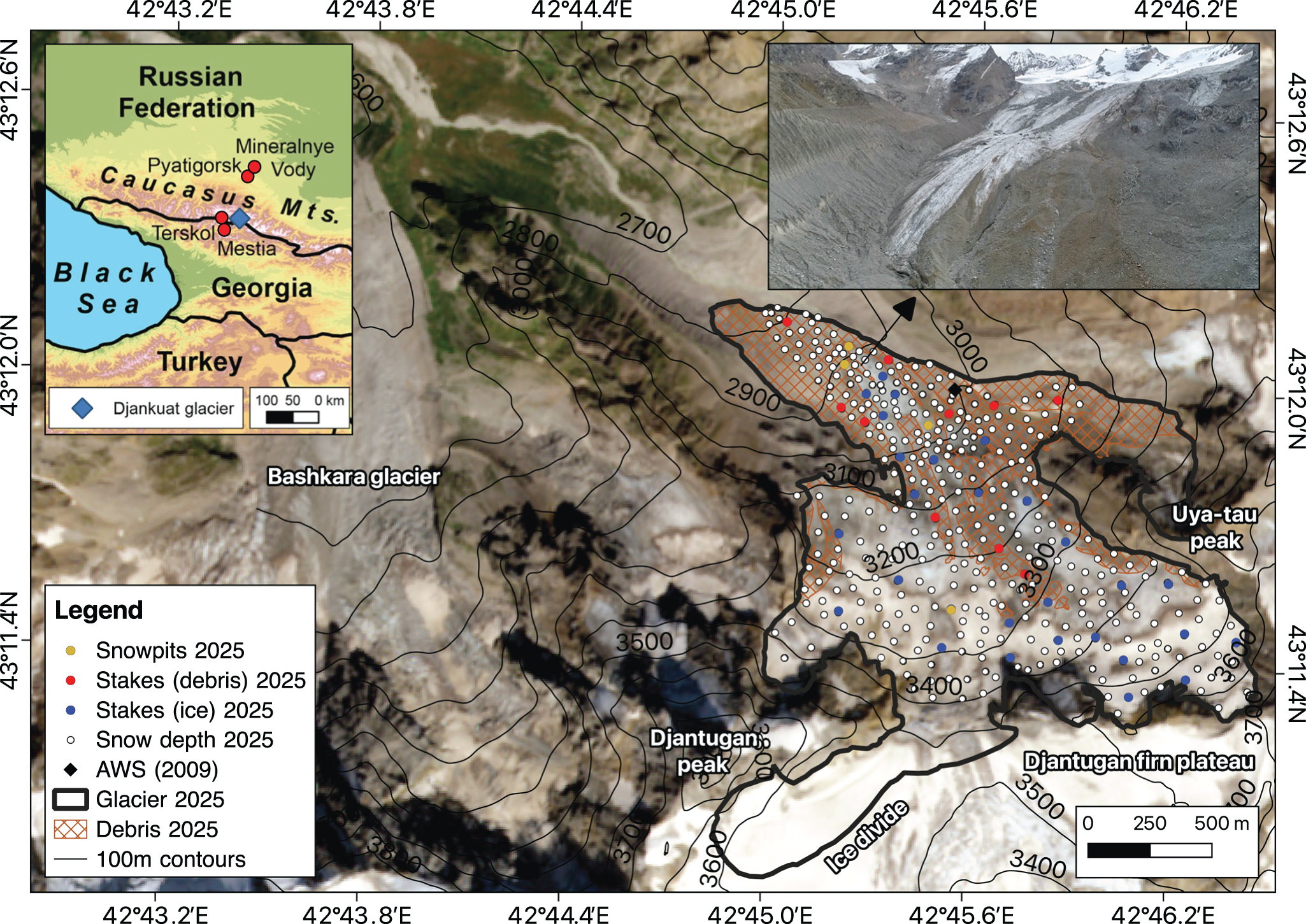
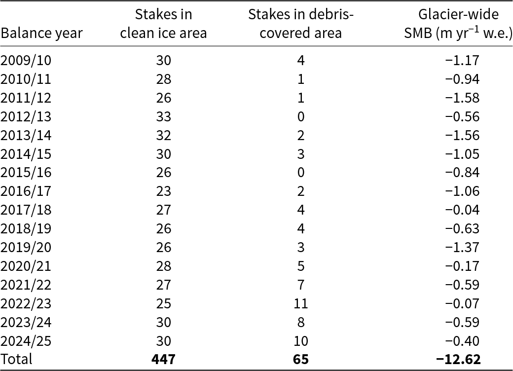
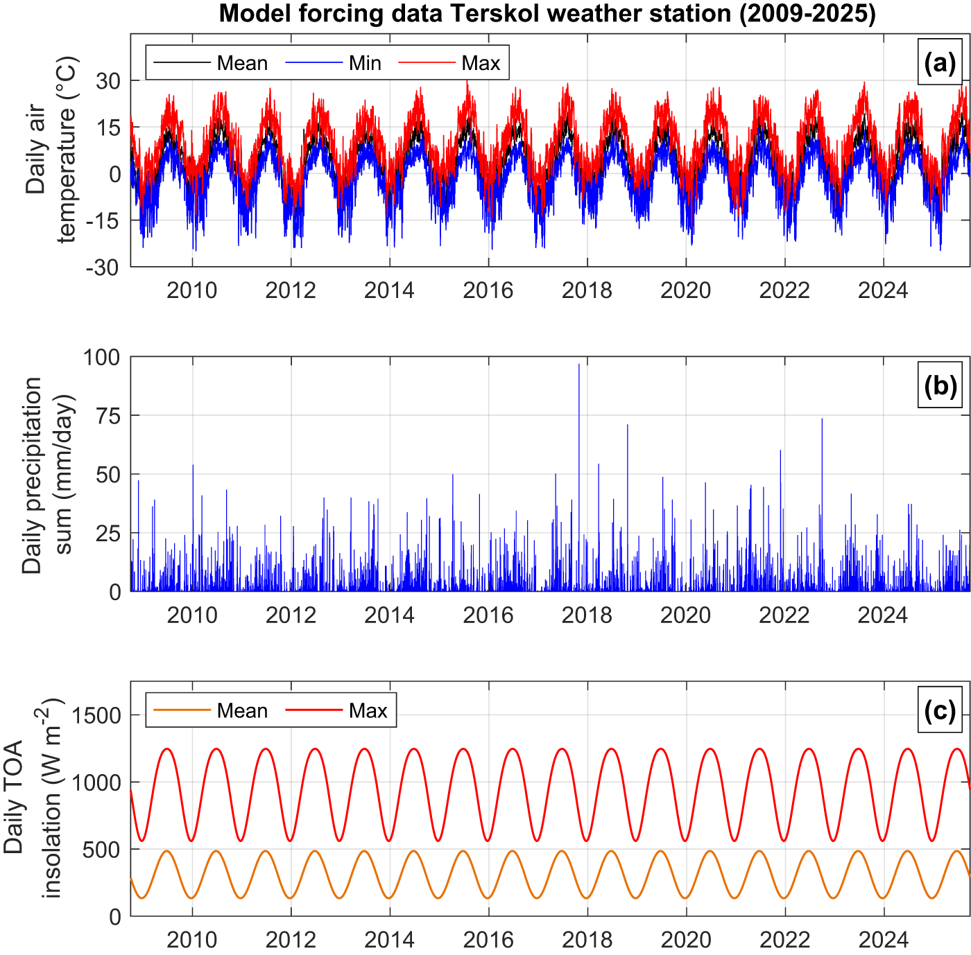


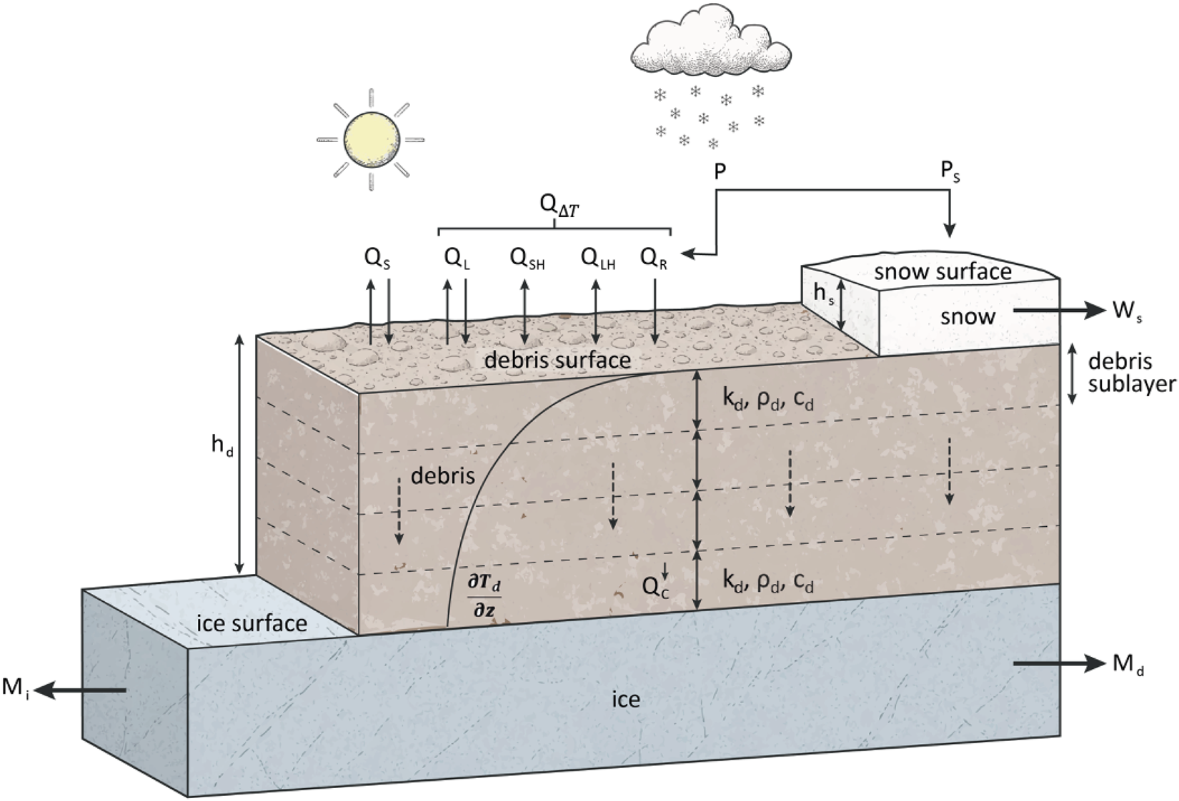

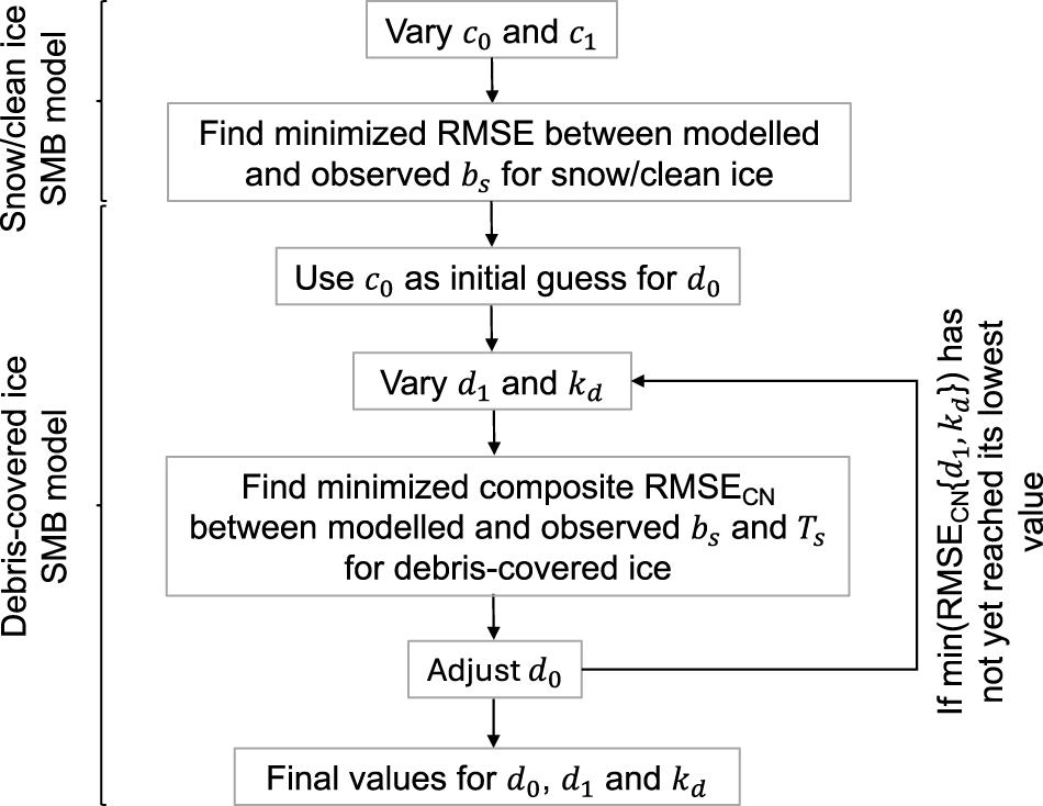
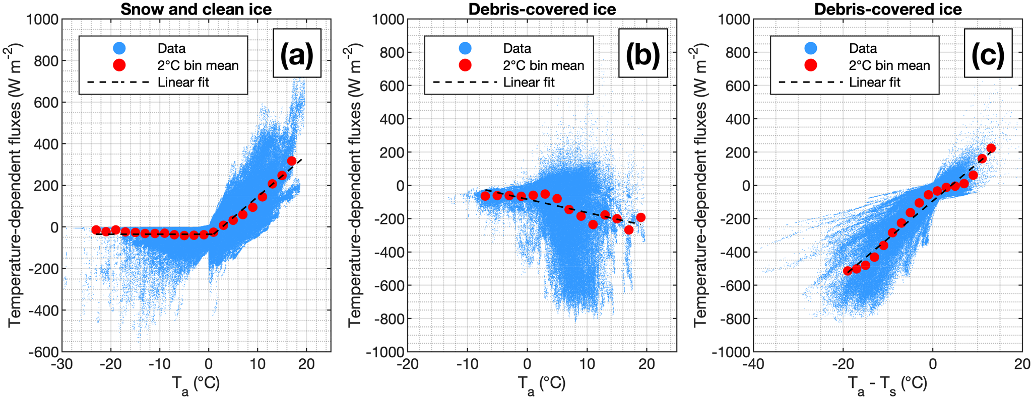

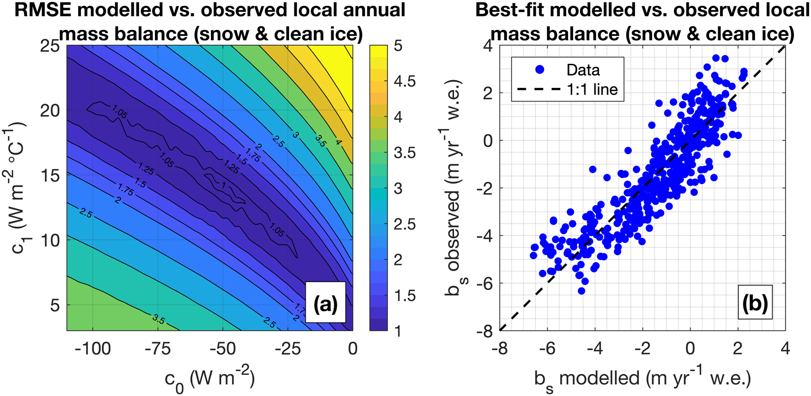


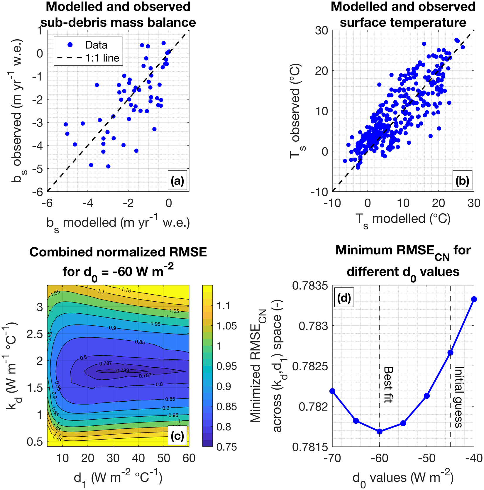


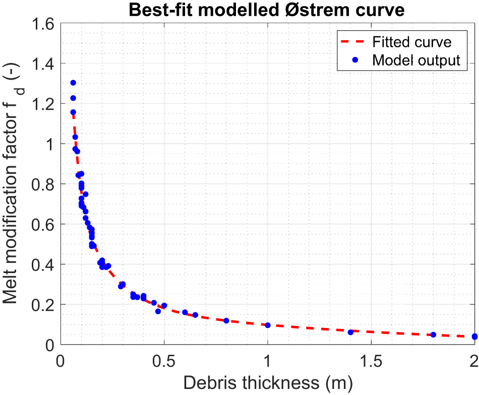
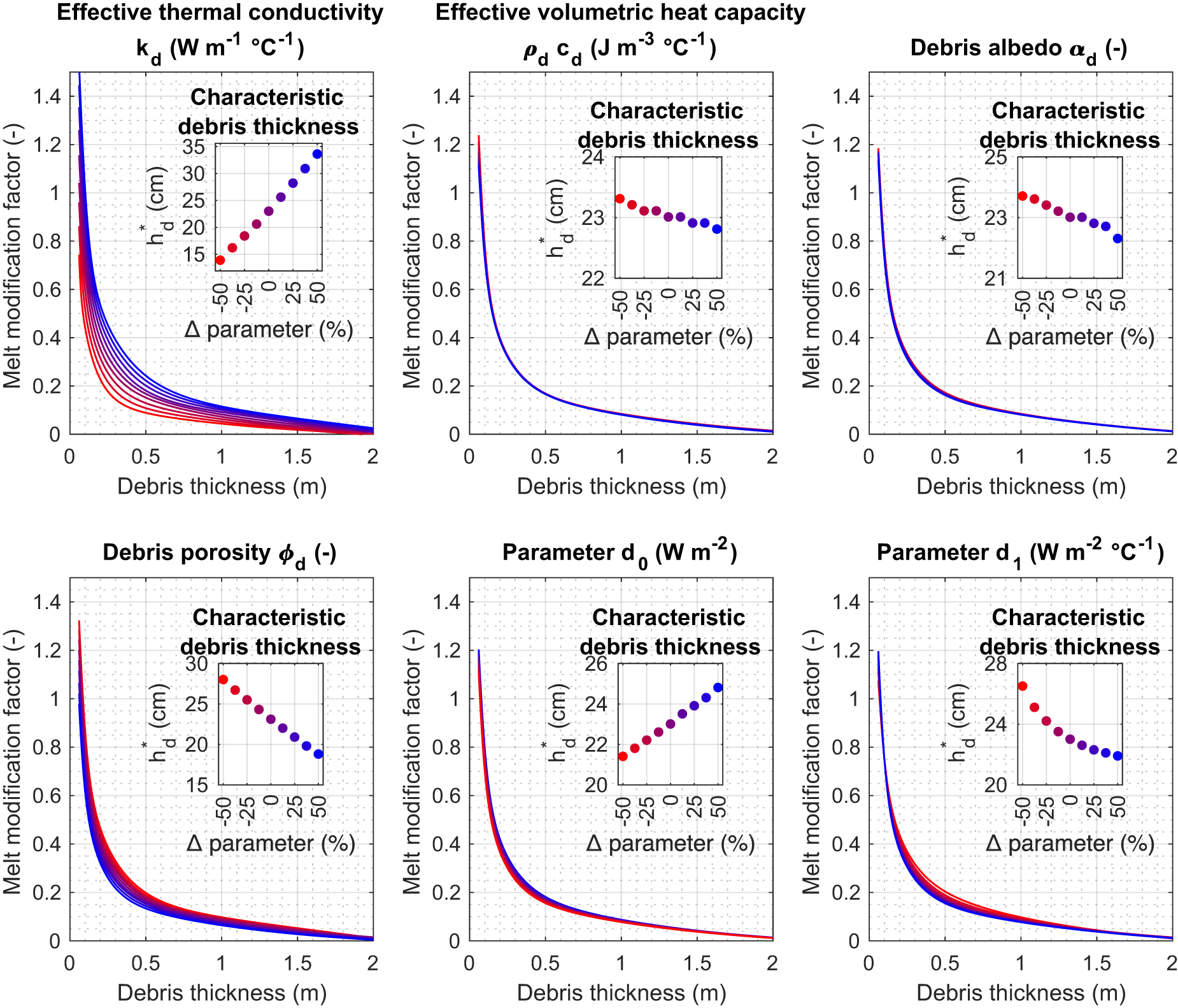


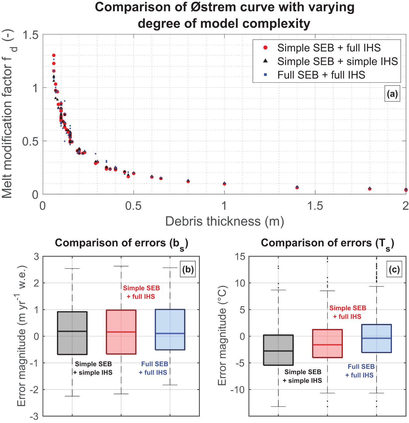
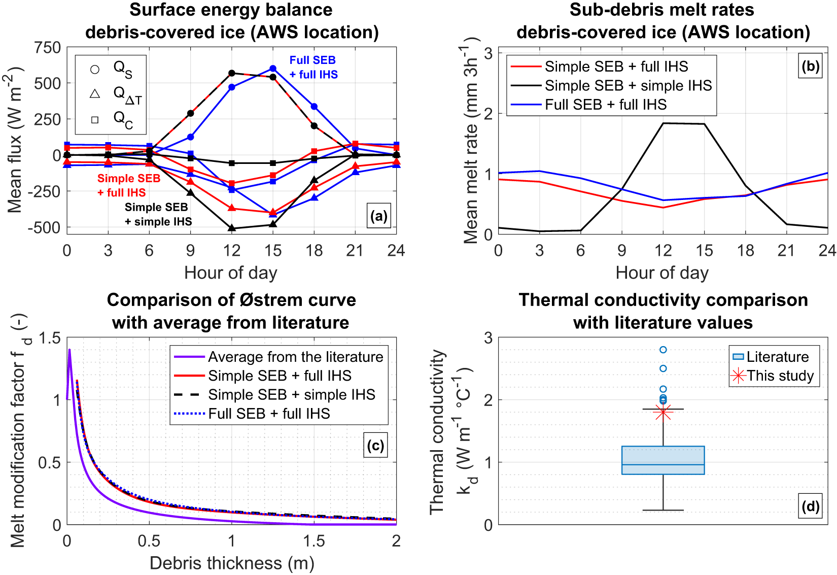


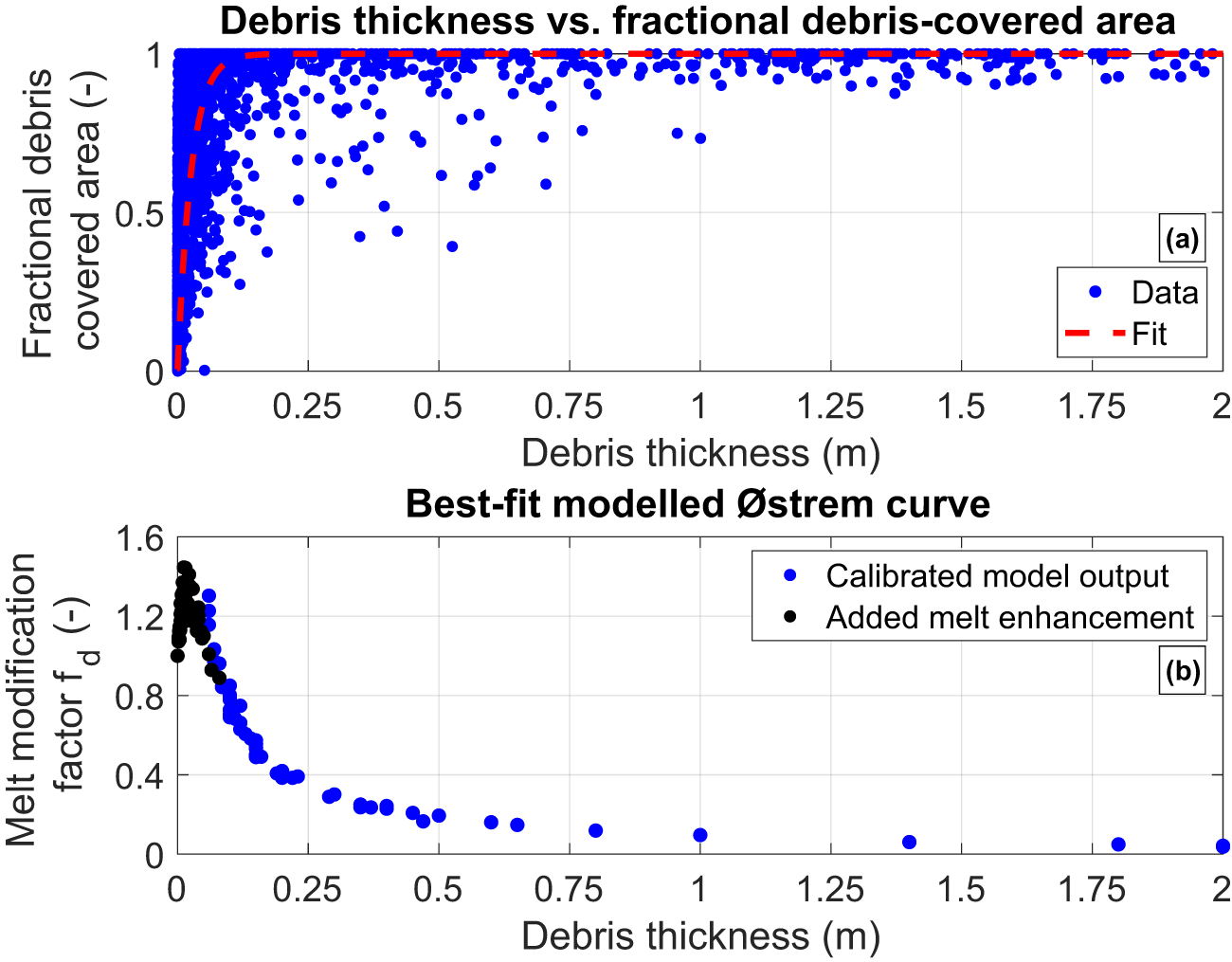
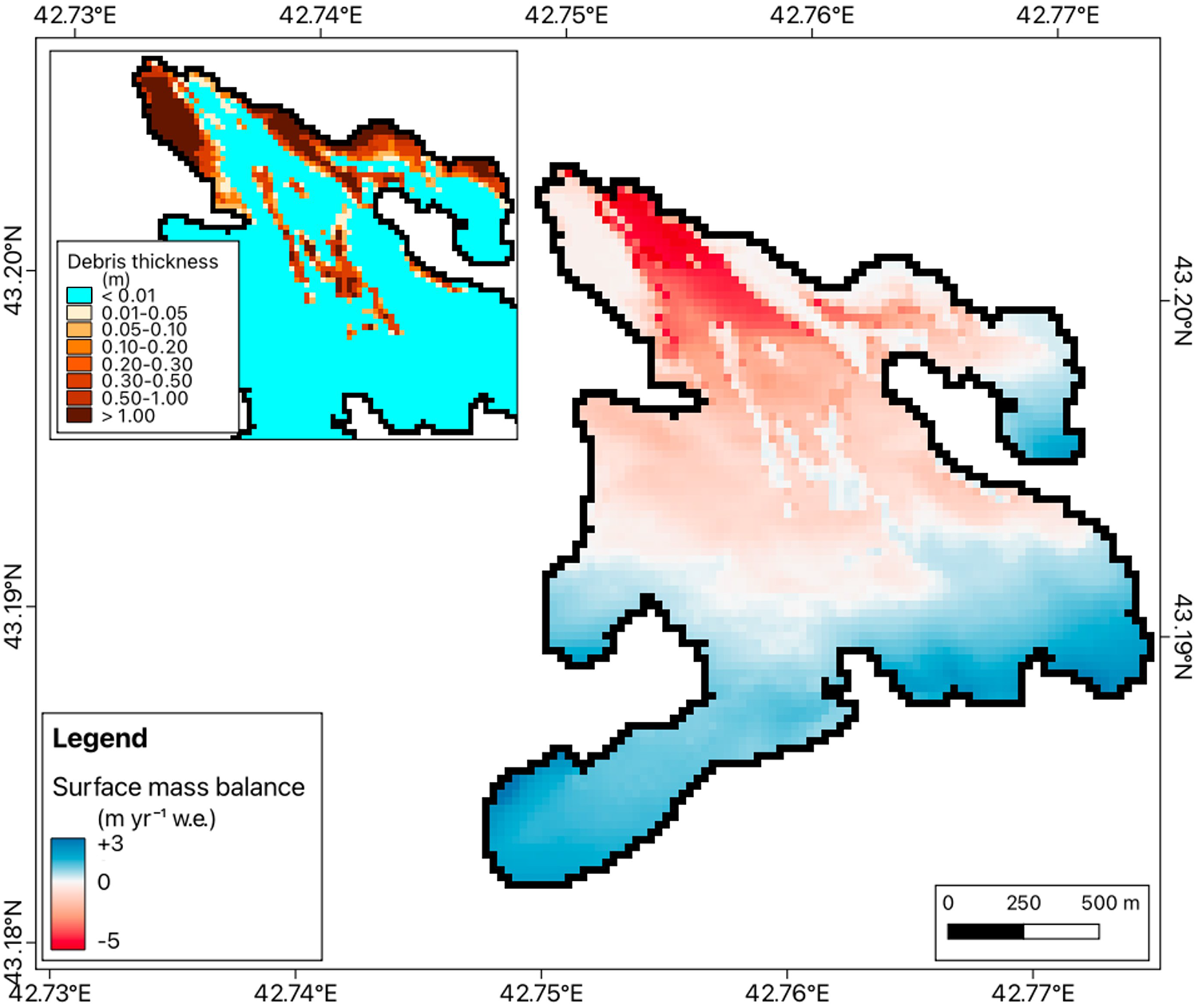

 Open access

