





1. Introduction
A turbulent jet is negatively buoyant when its buoyancy directly opposes its momentum. It will continually decelerate until its mean momentum is reduced to zero and the fluid reverses direction, returning towards the source while mixing with the opposing fluid. These occur in various industrial applications, such as building ventilation and brine discharge in desalination plants (Pincince & List Reference Pincince and List1973; Baines, Turner & Campbell Reference Baines, Turner and Campbell1990), as well as natural phenomena, including explosive volcanic jets and cumulonimbus convection in the atmosphere (Berson & Baird Reference Berson and Baird1975; Carazzo, Kaminski & Tait Reference Carazzo, Kaminski and Tait2008). Some time after the initial rise of a negatively buoyant jet, the flow reaches a quasi-steady state, where it oscillates around its steady state height,  $z_{ss}$, which is lower than the maximum height reached during its initial rise, the initial rise height,
 $z_i$. This quasi-steady state stage of the flow is referred to as the ‘fully developed fountain’ stage, with a structure consisting of an inner flow (IF) surrounded by an opposing annular outer flow (OF) (Turner Reference Turner1966; McDougall Reference McDougall1981; Mizushina et al. Reference Mizushina, Ogino, Takeuchi and Ikawa1982). Prior to the fully developed fountain forming, during the initial rise to
 $z_i$, there is no OF and the flow structure resembles a turbulent jet or plume. This will be referred to as the ‘negatively buoyant jet’ stage of the flow, and is the primary focus of the present investigation.
For a round inlet,  $z_i$ and
 $z_{ss}$ are governed by the source Froude or Richardson numbers,
 $Fr_o$ and
 $Ri_o$,
 \begin{equation} Fr_o = \frac{w_o}{(-r_o b_o)^{1/2}} = \frac{1}{(-Ri_o)^{1/2}}, \end{equation}
where  $w_o$ and
 $r_o$ are the initial average axial velocity and source radius, and
 $b_o=g(\rho _o-\rho _e)/\rho _e$ is the source buoyancy. Here,
 $\rho$ is the fluid density and
 $g$ the gravitational acceleration, with subscripts
 $o$ and
 $e$ denoting the source and environment. This is applicable to ‘light’ jets ejected downwards into a denser ambient (
 $\rho _e>\rho _o$), which are considered ‘negatively buoyant’ since their buoyancy opposes their momentum. This definition of
 $Fr_o$ and
 $Ri_o$ means that for a negatively buoyant jet
 $Fr_o>0$ and
 $Ri_o<0$, as convention, since
 $b_o<0$. It may also be noted that this definition of
 $Ri_o$ can also be used for positively buoyant jets/plumes (
 $Ri_o>0$), but the
 $Fr_o$ in this context is reserved for negatively buoyant jets only (
 $b_o<0$). For a negatively buoyant jet with high source Reynolds and Froude numbers (
 $Fr_o\gtrsim 5.5$),
 $z_{ss}$ and
 $z_i$ have been shown to follow
 $z_{ss}/r_o=2.46Fr_o$, with
 $z_i/z_{ss}=1.45$ (Turner Reference Turner1966; Burridge & Hunt Reference Burridge and Hunt2012). Here the source Reynolds number is defined as
 $Re_o=w_oD/\nu _o$ with
 $\nu _o$ denoting the kinematic viscosity of the source fluid and
 $D=2r_o$ is the source diameter. For weak fountains,
 $1.0\lesssim Fr_o\lesssim 1.7$, the initial rise height is actually lower than the steady state height,
 $z_{i}\lesssim z_{ss}$ (Burridge & Hunt Reference Burridge and Hunt2012), and a different
 $Fr_o$ relation is followed. However, these are not considered in the present investigation, which is primarily focused on the high
 $Fr_o$ regime.
Turner (Reference Turner1966) used dimensional arguments to derive the linear  $Fr_o$ scaling for the initial rise height of a negatively buoyant jet. More recent experimental efforts, relying on bulk measurements of the initial and steady state rise heights, have classified different negatively buoyant jet/fountain regimes based on
 $Fr_o$, with lower
 $Fr_o$ flows having a nonlinear relationship between
 $z_i$ and
 $Fr_o$ (Kaye & Hunt Reference Kaye and Hunt2006; Burridge & Hunt Reference Burridge and Hunt2012). In addition to rise height, it is also useful to be able to measure and predict overall entrainment and dilution in fountains, which is of significant importance to the application of brine discharge in desalination plants, where dilution levels are crucial to mitigating ecosystem damage (Pincince & List Reference Pincince and List1973). Burridge & Hunt (Reference Burridge and Hunt2016) took bulk measurements of the total entrained volume flux of fountains with different
 $Fr_o$, finding different scaling relations across the various
 $Fr_o$ classifications. Kaminski, Tait & Carazzo (Reference Kaminski, Tait and Carazzo2005) also used bulk measurements to investigate entrainment, but specific for the initial rise stage, where they found evidence that entrainment may be significantly reduced in negatively buoyant jets compared to neutral jets.
Studies relying on bulk measurements, however, are unable to provide detailed information about the internal structure of negatively buoyant jets/fountains. Mizushina et al. (Reference Mizushina, Ogino, Takeuchi and Ikawa1982) used constant temperature and current anemometry to obtain velocity and temperature measurements inside of high  $Fr_o$ fountains, finding temperature profiles similar to a neutral jet, and that the inner velocity profile was similar but wider. Mizushina et al. (Reference Mizushina, Ogino, Takeuchi and Ikawa1982) also found that the mean velocity and temperature profiles, and the turbulence intensities, were not self-similar. Cresswell & Szczepura (Reference Cresswell and Szczepura1993) investigated fully developed fountains with
 $Fr_o\cong 3.2$ using laser Doppler anemometry and thermocouples to obtain velocity and temperature measurements. They reported high shear stresses at the IF/OF boundary and in the cap region, and found that velocity–temperature correlations in the OF were similar to those in pure plumes. They also found that the flow in general could not be described by self-similar profiles. More recently, Williamson, Armfield & Lin (Reference Williamson, Armfield and Lin2011) undertook direct numerical simulations for
 $Fr_o=4$ and
 $7$ fountains, also finding that the profiles were not generally self-similar. Additionally, Williamson et al. (Reference Williamson, Armfield and Lin2011) found that other than during a short region near the source, fluid is primarily ejected from the IF to the OF, indicating ‘negative entrainment’ with respect to the IF, for
 $Fr_o=7$ fountains. This observation of radial outflow from the IF to OF was also made by Cresswell & Szczepura (Reference Cresswell and Szczepura1993) after an axial distance of
 $1.3r_o$ for a
 $Fr_o\cong 3.2$ fountain.
Another approach to investigating negatively buoyant jets and fountains is to use the existing integral models originally developed by Morton, Taylor & Turner (Reference Morton, Taylor and Turner1956) and Priestley & Ball (Reference Priestley and Ball1955) to describe neutral/positively buoyant jets and plumes. The Morton et al. (Reference Morton, Taylor and Turner1956) model is based on the conservation of volume and momentum, while the Priestley & Ball (Reference Priestley and Ball1955) model is based on the conservation of mean kinetic energy and momentum. Both approaches can make use of the ‘entrainment assumption’, which relates the radial velocity of fluid entrained into the jet/plume, to a characteristic vertical velocity at that height by the entrainment coefficient,  $\alpha$ (Morton et al. Reference Morton, Taylor and Turner1956; Fox Reference Fox1970). Papanicolaou, Papakonstantis & Christodoulou (Reference Papanicolaou, Papakonstantis and Christodoulou2008) applied this model to negatively buoyant jets and compared the prediction of initial rise height to bulk measurements of
 $z_i$ obtained experimentally. They found that a reduced entrainment coefficient (compared to neutral jets) is required for the model to match their experimental observations.
Other integral models aimed at describing the fully developed fountain case have also been developed, such as by McDougall (Reference McDougall1981) and Bloomfield & Kerr (Reference Bloomfield and Kerr2000), who modelled a fountain as an upwards flowing negatively buoyant jet, surrounded by a descending annular line plume. This approach requires estimating entrainment between the IF/OF and OF/ambient fluid, as well as characterising the top (or ‘cap’) of the fountain. Bloomfield & Kerr (Reference Bloomfield and Kerr2000) produced four variations of their model, but found that all of the models under-predicted the steady state rise height of the fountains compared to experimental data.
The application of integral model approaches to negatively buoyant jets, both for the initial rise and the fully developed fountain (e.g. McDougall Reference McDougall1981; Bloomfield & Kerr Reference Bloomfield and Kerr2000; Carazzo, Kaminski & Tait Reference Carazzo, Kaminski and Tait2010), has been hampered by a lack of data of the IF structure. If these integral models are to be more successful, a better understanding of the effect of negative buoyancy on turbulent jets (without a return flow) is a necessary and important step, although is likely still insufficient in fully modelling a fountain. A key aim of this investigation is therefore to contribute to an improved understanding of how negative buoyancy affects entrainment and the development of turbulent jets more generally. The present research focuses on the initial transient jet, obtaining data experimentally using combined two-dimensional particle image velocimetry (PIV) and planar laser induced fluorescence (PLIF). Additional background regarding the integral models is provided in § 2, followed by an outline of the experimental method in § 3. Mean statistics are presented in §§ 4 and 5, including discussion regarding the scaling of the mean and turbulence profiles with axial distance. Entrainment along the negatively buoyant jet is investigated in § 6, and the spreading rate of the velocity and buoyancy profiles is discussed in § 7. Both entrainment and the spreading rates are found to differ significantly from neutral jets and plumes, but nevertheless can be explained by the same governing conservation equations.
2. Integral models
The early integral models developed by Morton et al. (Reference Morton, Taylor and Turner1956) and Priestley & Ball (Reference Priestley and Ball1955), henceforth referred to as the MTT and PB models, may be expressed in terms of the volume, momentum and buoyancy flux,  $Q$,
 $M$ and
 $F$, and the integral buoyancy,
 $B$,
 \begin{equation} Q = 2\int_{0}^{\infty}\bar{w}r\,\mathrm{d}r, \quad M = 2\int_{0}^{\infty}\bar{w}^2r\,\mathrm{d}r, \quad F = 2\int_{0}^{\infty}\bar{w}\bar{b}r\,\mathrm{d}r, \quad B = 2\int_{0}^{\infty}\bar{b}r\,\mathrm{d}r, \end{equation}
where the vertical coordinate is denoted by  $z$, and corresponds to the axial velocity,
 ${w=w(z,r)}$, which can be decomposed into its mean (ensemble averaged) and fluctuating components
 ${w=\bar {w}+w'}$. The radial coordinate is
 $r$ and similarly corresponds to the radial velocity,
 $u$, and
 ${b=g(\rho -\rho _e)/\rho _e}$ is the buoyancy. Note that to obtain the physical fluxes in the flow, (2.1a–d) must be scaled by a factor of
 ${\rm \pi}$. These integral quantities can be used to define the following characteristic velocity, width and buoyancy for the jet,
 \begin{equation} w_m = \frac{M}{Q}, \quad r_m = \frac{Q}{M^{1/2}}, \quad b_m = \frac{BM}{Q^2} = \frac{F}{\theta_m Q}, \end{equation}
where  $\theta _m$ is defined in (2.8). These allow local Froude and Richardson numbers to be defined,
 $Fr$ and
 $Ri$, which depend on the local scales at any given
 $z$, and so may change along the length of the jet,
 \begin{equation} Fr = \frac{w_m}{(-r_m b_m)^{1/2}} = \frac{1}{(-Ri)^{1/2}}. \end{equation}
Due to the definition of  $b$, the above expression for
 $Fr$ is only valid for ‘light’ jets injected downwards into a more dense environment (
 $\rho _e>\rho$).
For an axisymmetric turbulent jet with arbitrary buoyancy, the following equations based on the conservation of volume, streamwise specific momentum, buoyancy and mean kinetic energy may be derived for flow into a uniform unstratified environment. These invoke the Boussinesq approximation, assume high Reynolds number flow, neglect the pressure contributions in the momentum and mean energy equations (van Reeuwijk & Craske Reference van Reeuwijk and Craske2015),
 \begin{gather} \frac{\mathrm{d}Q}{\mathrm{d}z} = 2\alpha M^{1/2}, \end{gather}
 \begin{gather}\frac{\mathrm{d}}{\mathrm{d}z}(\beta_g M) = \frac{FQ}{\theta_m M} = B, \end{gather}
 \begin{gather}\frac{\mathrm{d}}{\mathrm{d}z}\left(\frac{\theta_g}{\theta_m}F\right) = 0, \end{gather}
 \begin{gather}\frac{\mathrm{d}}{\mathrm{d}z}\left(\gamma_g\frac{M^2}{Q}\right) = \delta_g \frac{M^{5/2}}{Q^2} + 2F. \end{gather}
Here,  $\beta$,
 $\gamma$,
 $\delta$ and
 $\theta$ are the ‘profile coefficients’ defined in (2.8), where subscripts
 $m$ and
 $f$ correspond to the mean and turbulent components respectively, and subscript
 $g$ indicates the sum of them both,
 \begin{equation}
\left. \begin{array}{c@{}} \displaystyle \beta_m =
\dfrac{M}{w_m^2r_m^2} = 1,\quad \beta_f =
\dfrac{2}{w_m^2r_m^2}\int_{0}^{\infty}\overline{w'^2}r\,\mathrm{d}r,
\\ \displaystyle \gamma_m =
\dfrac{2}{w_m^3r_m^2}\int_{0}^{\infty}\bar{w}^3
r\,\mathrm{d}r,\quad \gamma_f =
\dfrac{4}{w_m^3r_m^2}\int_{0}^{\infty}\bar{w}\overline{w'^2}r\,\mathrm{d}r,\\
\displaystyle \delta_m =
\dfrac{4}{w_m^3r_m}\int_{0}^{\infty}\overline{w'u'}\dfrac{\partial\bar{w}}{\partial
r}r\,\mathrm{d}r, \quad \delta_f =
\dfrac{4}{w_m^3r_m}\int_{0}^{\infty}\overline{w'^2}\dfrac{\partial\bar{w}}{\partial
z}r\,\mathrm{d}r, \\ \displaystyle \theta_m =
\dfrac{F}{w_mb_mr_m^2}, \quad \theta_f =
\dfrac{2}{w_mb_mr_m^2}\int_{0}^{\infty}\overline{w'b'}r\,\mathrm{d}r.
\\ \displaystyle \beta_g = \beta_m + \beta_f, \quad
\gamma_g = \gamma_m + \gamma_f, \quad \delta_g = \delta_m +
\delta_f, \quad \theta_g = \theta_m + \theta_f.
\end{array}
\right\}\end{equation}
By observing the definitions of these profile coefficients, and their role in (2.5)–(2.7), we see that  $\beta$,
 $\gamma$,
 $\delta$ and
 $\theta$ are the dimensionless momentum flux, mean energy flux, turbulence production and buoyancy flux (van Reeuwijk & Craske Reference van Reeuwijk and Craske2015). Note that for Gaussian velocity and buoyancy profiles,
 $\theta _m=2/(\lambda ^2+1)$, with,
 \begin{equation} \lambda = \frac{r_b}{r_w}, \end{equation}
where  $r_w$ and
 $r_b$ are the
 $1/e$ widths of the velocity and buoyancy profiles (Papanicolaou & List Reference Papanicolaou and List1988). For self-similar profiles,
 $\lambda$ is constant and is also equal to the ratio of half-widths, or any other similarly defined width.
The entrainment assumption, which relates the radial velocity of entrained fluid to a characteristic vertical velocity at that height by the entrainment coefficient,  $\alpha$, is defined here as (Morton et al. Reference Morton, Taylor and Turner1956; van Reeuwijk & Craske Reference van Reeuwijk and Craske2015),
 \begin{equation} (r\bar{u})|_{r=\infty} = -\alpha r_m w_m. \end{equation}
Although there is considerable scatter in the literature,  $\alpha$ has been shown to be constant for pure plumes and jets in the far field, where the velocity and buoyancy profiles are self-similar, and that entrainment is higher in plumes (
 $0.10\lesssim \alpha _p\lesssim 0.16$) than jets (
 $0.065\lesssim \alpha _j\lesssim 0.080$) (Fischer et al. Reference Fischer, List, Koh, Imberger and Brooks1979; Carazzo, Kaminski & Tait Reference Carazzo, Kaminski and Tait2006). For jets with both momentum and buoyancy,
 $\alpha$ has been shown to depend on the local Richardson number (Priestley & Ball Reference Priestley and Ball1955; Fox Reference Fox1970; Kaminski et al. Reference Kaminski, Tait and Carazzo2005; van Reeuwijk & Craske Reference van Reeuwijk and Craske2015). The simplest form of this relationship, originally derived by Fox (Reference Fox1970) and based on the PB model, may be written as,
 \begin{equation} \alpha = \alpha_j + (\alpha_p - \alpha_j)\frac{Ri}{Ri_p}, \end{equation}
where  $Ri_p=8\alpha _p\beta _g/5$ is the plume Richardson number (Priestley & Ball Reference Priestley and Ball1955; Fox Reference Fox1970; van Reeuwijk & Craske Reference van Reeuwijk and Craske2015). In this relation,
 $\alpha$ in positively buoyant jets takes values between that of pure jets (
 $\alpha =\alpha _j$ when
 $Ri=0$) and pure plumes (
 $\alpha =\alpha _p$ when
 $Ri=Ri_p$).
Papanicolaou et al. (Reference Papanicolaou, Papakonstantis and Christodoulou2008) applied (2.11) to negatively buoyant jets in their integral model, and compared the models prediction of rise height,  $z_i$, to bulk measurements of
 $z_i$ from experiments. They found that a significantly reduced constant value of the entrainment coefficient,
 $\alpha _{j}=0.057$, must be used in order to accurately predict
 $z_i$. Conversely, Bloomfield & Kerr (Reference Bloomfield and Kerr2000) assumed a constant entrainment coefficient and found that a larger value of
 $\alpha =0.085$ gave good predictions of
 $z_i$ compared to experiments in both homogeneous and stratified environments. Kaminski et al. (Reference Kaminski, Tait and Carazzo2005) took a different approach by calculating the ‘bulk entrainment’ of collapsing ethanol and ethylene glycol jets, and found a reduced value of
 $\alpha =0.057$. Although this is the same value found as Papanicolaou et al. (Reference Papanicolaou, Papakonstantis and Christodoulou2008), in the context of Kaminski et al. (Reference Kaminski, Tait and Carazzo2005) it corresponds to a ‘bulk’ value, while in Papanicolaou et al. (Reference Papanicolaou, Papakonstantis and Christodoulou2008) it corresponds to an upper limit for
 $\alpha$ when
 $Ri\rightarrow 0$, and decreases for more negative
 $Ri$ (further along the jet). These studies have all used bulk measurements of the flow, typically rise height, to compare with predictions of the integral models. There have been few attempts to obtain local measurements of the internal velocity and buoyancy fields of negatively buoyant jets, which would provide an alternative approach to assessing the validity of using these models.
2.1. Morton's (Reference Morton1959) analytical solution
Morton (Reference Morton1959) further assumed self-similar Gaussian velocity and buoyancy profiles, a constant entrainment coefficient and considered only the mean components of the profile coefficients (subscript  $m$), to obtain (2.12a–c),
 \begin{equation} \frac{\mathrm{d}Q}{\mathrm{d}z} = 2\alpha M^{1/2},\quad \frac{\mathrm{d}M}{\mathrm{d}z} = \frac{FQ}{\theta_mM},\quad \frac{\mathrm{d}F}{\mathrm{d}z} = 0. \end{equation}
In this case, all of the profile coefficients in (2.8) are constants, and an analytical solution was derived for a positively or negatively buoyant jet originating from a point source. The solution to this system of equations is plotted here in figure 1 for the case of a negatively buoyant jet ( $F<0$). The following new variables are used to interpret the solution,
 \begin{gather} q =\alpha^{-1/2}\theta_m^{-1/2}|F_o|^{1/2} |M_o|^{-5/4}Q, \end{gather}
 \begin{gather}m = \frac{M}{|M_o|}, \end{gather}
 \begin{gather}\zeta = 2\alpha^{1/2}\theta_m^{-1/2}|F_o|^{1/2} |M_o|^{-3/4}z, \end{gather}
where the constant  $M_o$ is the initial momentum flux at the point source and
 $F_o=F$ is the buoyancy flux. Integral velocity, width and buoyancy scales can be defined based on the above variables (Morton Reference Morton1959),
 \begin{equation} \hat{w}_m = \frac{m}{q}, \quad \hat{r}_m = \frac{q}{m^{1/2}}, \quad \hat{b}_m = \frac{1}{q}. \end{equation}
These variables allow new ‘scaled’ local Froude and Richardson numbers to be defined,
 \begin{equation} \widehat{Fr}=\frac{\hat{w}_m}{(\hat{r}_m\hat{b}_m)^{1/2}} = \frac{1}{\widehat{Ri}^{1/2}}. \end{equation}
The solution to (2.12) for a negatively buoyant jet originating from a point source is plotted against  $\zeta$ in figures 1(a) and 1(b) in terms of the integral scales defined in (2.16) (Morton Reference Morton1959). An additional term,
 $\hat H_2 = -{\hat r_m}/({2\hat w_m})({\mathrm {d}\hat w_m}/{\mathrm {d}\zeta })$, is plotted in figure 1(c) and is discussed in more detail in § 7. The velocity scale,
 $\hat {w}_m$, decreases with
 $\zeta$ until it reaches its maximum height at
 $\zeta _i=1.454$ where
 $\hat {w}_m=0$ and
 $\widehat {Fr}=0$. Here, the width scale,
 $\hat {r}_m$, approaches infinity and the buoyancy scale decreases to a finite value,
 $\hat {b}_m=0.791$. Figure 1(b) reveals that
 $1/\hat {w}_m$,
 $1/\hat {b}_m$ and
 $\hat {r}_m$ increase approximately linearly with
 $\zeta$ for
 $\zeta \lesssim 0.5$ (
 $\widehat {Fr}\gtrsim 2$), implying that the velocity and buoyancy scales are nearly proportional to
 $\zeta ^{-1}\sim z^{-1}$, and radial scale to
 $\zeta \sim z$, in the lower portion of the jet. Although
 $\hat w_m$,
 $\hat b_m$ and
 $\hat r_m$ all change continuously along the negatively buoyant jet, the flow may still be characterised as consisting of two separate regimes. A ‘forced regime’ where the scales may be approximated as linear with
 $\zeta$ (for
 $\zeta \lesssim 0.5$,
 $\widehat {Fr}\gtrsim 2$), and a ‘buoyancy dominated’ regime where this approximation is no longer suitable. The
 $\widehat {Fr}\lesssim 2$ regime is characterised by the strong deceleration of the flow, which is captured by the non-dimensional term
 $\hat H_2$. This is plotted in figure 1(c) against
 $\widehat {Fr}$ for both a negatively buoyant jet (NBJ) and neutral jet (J). For
 $\widehat {Fr}\gtrsim 2$ in the NBJ,
 $\hat H_2$ is small and similar to the neutral jet value of
 $\hat H_2=0.5$, corresponding to the ‘forced’ regime. After this, for
 $\widehat {Fr}\lesssim 2$,
 $\hat H_2$ rapidly increases with decreasing
 $\widehat {Fr}$ as the flow is strongly decelerated, corresponding to the ‘buoyancy dominated’ regime.
The solution to the system of ordinary differential equations in (2.12) for the case when  $F<0$ (i.e. a NBJ). The solution assumes fully self-similar velocity and buoyancy profiles and a constant entrainment coefficient,
 $\alpha$, and is presented in terms of the integral buoyancy, velocity and width scales defined in (2.16). Plots of
 $\hat {b}_m$,
 $\hat {r}_m$,
 $\hat {w}_m$,
 $\widehat {Fr}$ and
 $\hat H_2 = -{\hat r_m}/({2\hat w_m})({\mathrm {d}\hat w_m}/{\mathrm {d}\zeta })$ against
 $\zeta$ are shown in (a). The quantities
 $1/\hat {b}_m$ and
 $1/\hat {w}_m$ are additionally plotted in (b), which, for relatively small
 $\zeta$, are approximately proportional to
 $\zeta$. The quantities
 $\hat {b}_m$,
 $1/\hat {r}_m$,
 $\hat {w}_m$ and
 $\hat H_2$ are plotted against
 $\widehat {Fr}$ in (c). For a neutral jet (J),
 $\hat H_2=0.5$ everywhere, which is also plotted in (c) as a horizontal line.

In the analytical solution for high  $Re_o$ self-similar neutral jets, which have
 $Fr=\infty$,
 $w_m$ scales with
 $z^{-1}$ exactly (Fischer et al. Reference Fischer, List, Koh, Imberger and Brooks1979), and so it may be expected that the velocity in self-similar, constant
 $\alpha$, NBJs scales in approximately the same way for sufficiently high local
 $Fr$ (i.e. in the forced regime). Similarly, the scalar concentration and width scales in a neutral jet are also proportional to
 $z^{-1}$ and
 $z$ respectively, just as is approximately true for
 $\hat {b}_m$ and
 $\hat {r}_m$ in the forced regime. Figure 1(c) also shows how these scales change with
 $\widehat {Fr}$, with
 $\hat {b}_m$,
 $1/\hat {r}_m$,
 $\hat {w}_m$ all scaling approximately linearly for high
 $\widehat {Fr}$.
The present experimental results show that, even in the forced regime ( $\zeta \lesssim 0.5$,
 $\widehat {Fr}\gtrsim 2$), there are significant differences between the behaviour of NBJs and what is captured in this simplified model. These include turbulence intensities and shear stress that scale differently to the mean flow, discussed in §§ 4.3 and 5, a non-constant entrainment coefficient discussed in § 6, and the spreading of the velocity and buoyancy profiles discussed in § 7. Although these effects can be distinguished from each other, as are shown in the following sections they are also linked. For example, the turbulence intensities and shear stress have an effect on both entrainment and the spreading rate, as is discussed in §§ 6 and 7.
3. Experiments
The flow was investigated experimentally using combined two-dimensional PIV and PLIF, with a  $532$ nm Nd:YAG laser and four pco.2000 cameras. Two cameras were used for PIV and PLIF each, and then the images ‘stitched’ together, allowing for a larger region of interest (approximately
 $120\ \textrm {mm}^2 \times 60\ \textrm {mm}^2$). The stitching was performed using world-coordinate data obtained from a ‘target sheet’ image taken prior to the experiment. The target sheet consists of a checker-board pattern of squares with known dimensions and a reference circle. Processing this image allowed world coordinates to be obtained for each pixel in the image, which could be used to align and stitch the images. The PIV images were processed using the MATLAB package PIVSuite by J. Vejrazka, with a multi-pass interrogation and a final window size of
 $24\ \textrm {pixels}^2 \times 24\ \textrm {pixels}^2$ (
 $0.78\ \textrm {mm}^2 \times 0.78\ \textrm {mm}^2$) with a
 $75\,\%$ overlap. The PLIF images were processed using an algorithm developed by the present authors, which included a laser correction procedure that accounted for variations in the laser power profile between pulses. Rhodamine dye was chosen as the scalar tracer for the PLIF measurements since it has a high absorption rate near the laser wavelength (Zehentbauer et al. Reference Zehentbauer, Moretto, Stephen, Thevar, Gilchrist, Pokrajac, Richard and Kiefer2014), and has a high Schmidt number of
 $Sc\cong 2500$ (Gendron, Avaltroni & Wilkinson Reference Gendron, Avaltroni and Wilkinson2008; Vanderwel & Tavoularis Reference Vanderwel and Tavoularis2014). Further details of the experimental and image processing procedures are discussed in Milton-McGurk et al. (Reference Milton-McGurk, Williamson, Armfield and Kirkpatrick2020), Talluru et al. (Reference Talluru, Armfield, Williamson, Kirkpatrick and Milton-McGurk2020).
The flow was obtained using a  $1$ m
 $^3$ tank containing salt water, and injecting a source solution of freshwater, ethanol and Rhodamine 6G dye vertically from above through a round pipe (
 $D=5$ mm and
 $10$ mm) with entry lengths
 $\geq 75D$. Since the source mixture was lighter than the ambient salt water, its buoyancy forces oppose the downward motion of the jet and a NBJ is produced. The source fluid would descend into the tank during the initial flow stage, then reverse direction and move towards the free surface forming a return flow. The NBJ stage was defined as the initial stage where there is no return flow present, and the flow structure resembles that of a neutral jet or plume. During a single run, images were taken primarily during this initial stage, after which the flow was stopped. Typically between
 $6$ and
 $20$ runs were conducted at each axial location so that a sufficient number of images of this initial stage could be captured in order to obtain statistical convergence. A graphical illustration of the experimental set-up is given in figure 2.
Graphical illustration of the experimental set-up.

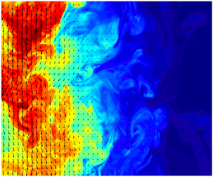
A schematic of the NBJ, and an example of a processed image, is shown in figure 3. All negatively buoyant jet runs had a source Froude and Reynolds numbers of  $Fr_o=30$ and
 $5500\lesssim Re_o\lesssim 5900$, with measurements taken for
 $18\lesssim z/D\lesssim 39$ using a
 $D=10$ mm pipe. Neutral jet measurements with the same pipe and
 $Re_o$ were obtained for
 $18\lesssim z/D\lesssim 30$, as well as using a smaller
 $D=5$ mm pipe so that a higher
 $Re_o\cong 10^4$ and
 $72\lesssim z/D\lesssim 78$ could be achieved.
Schematic of the NBJ with the laser sheet and region of interest indicated, and an example of a processed experimental image with the velocity vectors and scalar field shown. The region of interest is captured by two pairs of PIV and PLIF cameras, with the images stitched together to form a single image as shown.

Since the region of interest of the cameras was relatively small compared to the height of the jet/fountain ( $z_i\cong 535$ mm), the different stages of flow development were determined using velocity measurements of the inner structure. This involved observing how the volume flux in the IF (
 $Q_{IF}$) and OF (
 $Q_{OF}$) regions of the NBJ changed in time. These are defined as,
 \begin{equation} Q_{IF} = 2\int_{0}^{r_i} \tilde{w}r\mathrm{dr}, \quad Q_{OF} = 2\int_{r_i}^{\infty} \tilde{w}r\mathrm{dr}, \end{equation}
where  $r_i$ is the ‘boundary’ between the IF and OF and
 $\tilde {w}$ is the instantaneous axial velocity profile. Although the instantaneous boundary is likely to change in time, for the purposes of calculating
 $Q_{IF}$ and
 $Q_{OF}$,
 $r_i$ is taken as constant and defined as the first radial location where the mean velocity (calculated using all the instantaneous velocity profiles) is equal to zero. This notion of an IF/OF boundary may not be well defined at the top of the jet where the velocity goes to zero, but for the purposes of the present investigation it is sufficient to compute
 $Q_{IF}$ and
 $Q_{OF}$ prior to this region.
The ratio  $-Q_{OF}/Q_{IF}$ is plotted with time in figure 4 for a
 $Fr_o=30$ NBJ at
 $z/D\cong 19$. There are three distinct regions in figure 4, the first where
 ${-Q_{OF}/Q_{IF}\cong 0}$ and is approximately constant (since
 $Q_{OF}\ll Q_{IF}$), then a second, when the ratio rapidly increases then decreases and a third region where it oscillates around a value
 $-Q_{OF}/Q_{IF}\cong 2$. Images showing the velocity vectors and scalar concentration fields from these stages are given in figures 5(a)–5(c). The first stage, shown in (a), corresponds to the initial rise of the jet before the return flow has developed, and thus the velocity vectors are primarily orientated downwards (the positive
 $z$ direction) inside the jet, and have vertical components of approximately zero outside of it. The second stage, shown in (b), corresponds to the intermediate transient period after the NBJ has reached its maximum height as it begins collapsing back onto itself, but before it reaches the quasi-steady state of a fully developed fountain. Here the axial velocity of the IF reduces and a significant return flow begins to form, evident from the velocity vectors pointing towards the source (upwards in this figure) in the OF, where it was previously a nearly quiescent environment in (a). The fully developed fountain stage, shown in (c), does not look categorically different from the transient stage in the instantaneous images observed, with both images showing downward and upward flowing regions. However, as is shown in the
 $-Q_{OF}/Q_{IF}$ plot in figure 4, the volume flux in the IF and OF regions is much more steady in time during the fully developed stage. The shape of this plot, and the location of the three regions, are insensitive to the value of
 $r_i$ used in (3.1). For example, a similar plot is obtained if the velocity profile half-width, defined as the radial location where
 $\bar {w}/w_c=0.5$, is used. In the first region, where
 $-Q_{OF}/Q_{IF}$ is approximately constant, time-averaged profiles were computed and were found not to vary systematically in time. The flow could therefore be considered quasi-steady in this range, and so this was used to define the NBJ stage for each experiment. All NBJ statistics discussed in the following sections correspond to this initial stage. Additional details of this procedure are given in Milton-McGurk et al. (Reference Milton-McGurk, Williamson, Armfield and Kirkpatrick2020).
The ratio  $-Q_{OF}/Q_{IF}$, defined using (3.1), is plotted against time,
 $t$ (s). The ratio is a measure of the instantaneous volume flux in the IF and OF regions of a negatively buoyant jet/fountain, and is used to define the initial NBJ stage where
 $Q_{OF}\ll Q_{IF}$ and is approximately constant.

Three images showing the instantaneous velocity vectors and scalar concentration field of a NBJ as it develops into a fountain. With respect to figure 4, (a) was taken at approximately  $5$ s, (b) at
 $32$ s and (c) at
 $106$ s. These images correspond to the axial location range
 $17\lesssim z/D\lesssim 20$ where
 $z_{i}\cong 54D$, and are orientated such that that the jet core is flowing downwards (the positive
 $z$ direction).

4. Statistical description of the flow
4.1. Centreline decay
For a self-similar neutral jet with constant  $\alpha$, the decay of the centreline velocity along the jet axis follows the relation,
 \begin{equation} \frac{w_o}{\bar{w}_c} = K\left(\frac{z}{D} - \frac{z_o}{D}\right), \end{equation}
where  $w_o$ is the velocity at the source,
 $\bar {w}_c$ is the velocity at the jet centreline,
 $z_o$ is a virtual origin and
 $K$ is a constant (Fischer et al. Reference Fischer, List, Koh, Imberger and Brooks1979; Papanicolaou & List Reference Papanicolaou and List1988; Hussein, Capp & George Reference Hussein, Capp and George1994). For a neutral jet, the centreline velocity therefore scales with
 $z^{-1}$. There is some variation in the literature for the value of the constant
 $K$, such as
 $K=0.17$ by Hussein et al. (Reference Hussein, Capp and George1994) or
 $K=0.149$ by Papanicolaou & List (Reference Papanicolaou and List1988), but a robust finding is the linear
 $w_o/\bar {w}_c$ relation with
 $z$. Figure 6 shows
 $w_o/\bar {w}_c$ plotted against
 $z/D$ for neutral and negatively buoyant jets. A linear fit of our neutral jet data gives
 $K=0.142$, in good agreement with Papanicolaou & List (Reference Papanicolaou and List1988). The virtual origin for the present experiments is found to be close to the actual source at
 $z_o/D=0.707$.
The quantity  $w_o$/
 $\bar {w}_c$ plotted against axial distance
 $z/D$, showing the decay of the centreline velocity for a neutral and negatively buoyant jet. Each cluster of points was obtained from a separate experiment with the same source Froude number (
 $Fr_o=30$ for the NBJ) and similar Reynolds numbers (
 $5500\lesssim Re_o\lesssim 5900$). The prediction of Morton's (Reference Morton1959) model for a constant
 $\alpha =0.0714$ and
 $\lambda =1.2$ is shown, as well as ‘model 2’, a linear model for
 $\alpha$ with
 $Ri$ using coefficients based on values found by Kaminski et al. (Reference Kaminski, Tait and Carazzo2005). Additionally, ‘model 1’, which assumes a linear relationship for
 $\delta _m$ with
 $Ri$, is also shown. These models are discussed further in § 6.

For the NBJ, the decay is not linear over the  $z/D$ range shown, and can be seen diverging from the neutral jet results for
 $z/D\gtrsim 18$. As
 $z/D$ increases the local
 $Fr$ decreases towards zero (and
 $Ri$ asymptotes to negative infinity), which may be interpreted as negative buoyancy playing an increasingly important role in decelerating the flow. However, for the points closest to the source, e.g. for
 $z/D\lesssim 26$ (
 $Fr\gtrsim 3.0$,
 $Ri\gtrsim -0.11$),
 $w_o/\bar {w}_c$ could be approximated as linear with
 $z$, although with a different slope to a neutral jet. This may be considered the ‘forced’ regime where the flow is more similar to a neutral jet, and is consistent with the arguments made in § 2 regarding the solution to Morton (Reference Morton1959) simplified model. Although this is a local regime based on local
 $Fr$, it may be compared to the classification of fountains by source Froude number,
 $Fr_o$, such as those suggested by Burridge & Hunt (Reference Burridge and Hunt2012). They classified
 $2.8\lesssim Fr_o\lesssim 5.5$ and
 $Fr_o\gtrsim 5.5$ as ‘forced’ and ‘highly forced’ fountains, which is consistent with the presently suggested local ‘forced’ regime of
 $Fr\gtrsim 3.0$.
4.2. Velocity and buoyancy profiles
Time-averaged profiles for axial velocity and buoyancy, where buoyancy is presented in terms of scalar concentration  $\bar {c}$, are given in figure 7(a,b), normalised by their centreline values and respective half-widths. Dimensionless concentration (
 $0\leq c\leq 1$) and buoyancy (mm s
 $^{-2}$) are related by a constant such that
 $b=c(\rho _o-\rho _e)g/\rho _e$. All NBJ profiles are close to Gaussian for the full range of local
 $Fr$ investigated,
 $1.85\lesssim Fr\lesssim 5.91$, and are similar to the profiles for neutral jets. This is despite the considerable deceleration of the mean flow in the NBJ compared to the neutral jet, as demonstrated in figure 6, showing that the profiles maintain a Gaussian shape even outside of the forced regime (
 $Fr\lesssim 3.0$).
Time-averaged axial velocity and scalar concentration (buoyancy) profiles, in (a) and (b) respectively, of a NBJ with different local Froude numbers. Neutral jet (J) data from the present experimental set-up are also shown ( $Re_o=5900$), as well as by Webster, Roberts & Ra'ad (Reference Webster, Roberts and Ra'ad2001), Wang & Law (Reference Wang and Law2002) and Darisse, Lemay & Benaïssa (Reference Darisse, Lemay and Benaïssa2015). The NBJ profiles were obtained using data from multiple experiments using the same pipe,
 $D=10$ mm, at the same source Froude number,
 $Fr_o=30$, and similar Reynolds number,
 $5500\lesssim Re_o\lesssim 5900$, while varying the location of the region of interest relative to the source. All velocity and scalar concentration points have been normalised by their respective centreline values,
 $\bar {w}_c$ and
 $\bar {c}_c$, and half-widths,
 $r_{1/2,w}$ and
 $r_{1/2,c}$.

The ratio of widths between the buoyancy/scalar and velocity profiles is given by  $\lambda$ and defined in (2.9). For neutral jets,
 $r_b$ corresponds to the
 $1/e$ width of the scalar profile, with values estimated in the literature ranging
 $1.15\lesssim \lambda \lesssim 1.30$ (Fischer et al. Reference Fischer, List, Koh, Imberger and Brooks1979; Wang & Law Reference Wang and Law2002; Ezzamel, Salizzoni & Hunt Reference Ezzamel, Salizzoni and Hunt2015), and is assumed to be constant in the far field where the flow is self-similar. As pointed out by Ezzamel et al. (Reference Ezzamel, Salizzoni and Hunt2015), discrepancies in the literature may be attributed to the distance from the source where the profiles were measured (e.g. if the jet has not fully developed), and that it is likely that source conditions play a role.
Figures 8(a) and 8(b) show  $\lambda$ plotted with axial distance and local
 $Ri$ for both the neutral and NBJs from the present experiments. The values for the neutral jet are reasonably constant, and have an average value of
 $\lambda =1.181$, in good agreement with
 $\lambda _j=1.189$ from Fischer et al. (Reference Fischer, List, Koh, Imberger and Brooks1979). The slight decreasing trend may be attributed to the jet still developing at this axial distance. For the NBJ,
 $\lambda$ is higher than the neutral jet and increases with axial distance over the range shown. From figure 8(b),
 $\lambda$ can be seen to be increasing almost immediately from
 $Ri\cong -0.04$ (
 $Fr\cong 5.0$) with more negative
 $Ri$, which is within the previously suggested ‘forced’ regime of
 $Ri\gtrsim -0.11$ (
 $Fr\gtrsim 3.0$). So even for relatively high local
 $Fr$, the velocity and buoyancy/scalar profile widths grow at different rates compared with a neutral jet.
The  $1/e$ width ratio between the buoyancy (or scalar) and velocity profiles,
 $\lambda =r_b/r_w$, for a NBJ and neutral jet (J). The data are plotted against axial distance normalised by source diameter
 $z/D$ in (a), and against the local
 $Ri$ in (b). At the source,
 $Fr_o=30$ (
 $Ri_o=-0.0011$), which decreases towards
 $Fr=0$ (
 $Ri\rightarrow -\infty$) at the top of the NBJ. In (b), the values for a neutral jet, which have
 $Ri=0$ everywhere, are shown as horizontal lines for clarity.

A varying  $\lambda$ can be interpreted as a type of ‘similarity drift’ of the velocity and buoyancy profiles, which has also been reported in jets and plumes that have not yet reached a state of full self-similarity (Kaminski et al. Reference Kaminski, Tait and Carazzo2005; Carazzo et al. Reference Carazzo, Kaminski and Tait2006; Ezzamel et al. Reference Ezzamel, Salizzoni and Hunt2015). The mechanism causing the increasing
 $\lambda$ with
 $z$ for negatively buoyant jets is discussed in § 7.
4.3. Turbulence statistics
Figures 9 and 10 show the profiles of the axial turbulence intensity,  $\overline {w'^2}/\bar {w}_c^2$, and the normalised Reynolds stress,
 $\overline {w'u'}/\bar {w}_c^2$. The profiles at
 $z/D=73$ for the neutral jet in figures 9(a) and 9(b) are in good agreement with both the best fit curve from Wang & Law (Reference Wang and Law2002) and data from Darisse et al. (Reference Darisse, Lemay and Benaïssa2015). This experiment used a smaller,
 $D=5$ mm, pipe so that measurements could be taken at a larger downstream distance relative to the source diameter, and a high
 $Re_o=10\ 700$ could be achieved. The flow in this experiment could therefore be expected to be fully developed and self-similar and so could be compared to similar experiments in the literature, such as Wang & Law (Reference Wang and Law2002) who had
 $Re_o=12\ 700$ and
 $40<z/D<80$. The remaining J profiles in figure 9 correspond to experiments using a
 $D=10$ mm pipe and have
 $Re_o=5900$ in order to closely match the source conditions of the NBJ experiments. These
 $18<z/D<27$ profiles are generally a little lower than the
 $z/D=73$ case since they may not be completely developed at this distance, but are nevertheless reasonably close and can be compared to a negatively buoyant jet at the same axial location.
Mean turbulent axial velocity fluctuations (a), and Reynolds stress (b), for the neutral jet (J) at three different axial locations, normalised by the local mean centreline velocity,  $\bar {w}_c^2$. The
 $z/D=18$,
 $23$ and
 $27$ profiles correspond to an experiment with
 $D=10$ mm and
 $Re_o=5900$. The
 $z/D=73$ profiles were obtained used
 $D=5$ mm and
 $Re_o=10\ 700$. The best fit curve from Wang & Law (Reference Wang and Law2002) (
 $40<z/D<80$) and the data from Darisse et al. (Reference Darisse, Lemay and Benaïssa2015) (
 $z/D=30$) for a neutral jet are also shown.

Mean turbulent axial velocity fluctuations (a), and Reynolds stress (b), for a NBJ at several axial locations, normalised by the local mean centreline velocity,  $\bar {w}_c^2$. The source conditions were
 $Fr_o=30$ and
 $5500\lesssim Re_o\lesssim 5900$ using
 $D=10$ mm, with data gathered across multiple experiments.

Figures 10(a) and 10(b) shows the normalised  $\overline {w'^2}$ and
 $\overline {w'u'}$ profiles of a NBJ at some of the same axial distances as the neutral jet in figure 9, as well as two additional further downstream locations. Despite some scatter in the data, there is a clear upwards trend for both the axial turbulence intensity and Reynolds stress relative to the centreline velocity with increasing axial distance, or equivalently, decreasing local
 $Fr$. This is most evident for the
 $Fr\lesssim 3.38$ profiles as the flow exits the ‘forced’ regime, and is particularly strong in the
 $\overline {w'^2}/\bar {w}_c^2$ plot shown in (a). This does not imply that the magnitude of
 $\overline {w'^2}$ or
 $\overline {w'u'}$ is increasing with distance, but is instead revealing that
 $\overline {w'^2}$ and
 $\overline {w'u'}$ do not decrease at the same rate as the mean flow. This is consistent with the qualitative description of a NBJ, where the mean velocity is reduced to zero at the top of the jet,
 $z_i$, but where we can still expect non-zero turbulence.
Cresswell & Szczepura (Reference Cresswell and Szczepura1993) also obtained  $\overline {w'^2}$ and
 $\overline {w'u'}$ profiles, but for a fully developed fountain with
 $Fr_o\cong 3.2$. When their data (originally presented normalised by source conditions) are normalised by the centreline velocity, the peak values also increase with axial distance from the source as the mean flow decelerates. Near to the source,
 $0.03\lesssim z/D\lesssim 1.7$, their peak values for the IF cover the range
 $0.05\lesssim \overline {w'^2}/\bar {w}_c^2\lesssim 0.2$ and
 $0.01\lesssim \overline {w'u'}/\bar {w}_c^2\lesssim 0.03$, which is broadly similar to the present values. However, the flow of Cresswell & Szczepura (Reference Cresswell and Szczepura1993) was at a much lower
 $Fr_o\cong 3.2$ and also included a return flow, and so is notably different to the present case of
 $Fr_o=30$ NBJs. The phenomenon of increasing turbulence intensities in a decelerating mean flow is not exclusive to NBJs/fountains. In a flow through a conical diffuser, for example, increasing turbulence fluctuations and shear stresses, relative to the local centreline velocity, can be seen with increasing axial distance as the flow expands and decelerates (Okwuobi & Azad Reference Okwuobi and Azad1973; Singh & Azad Reference Singh and Azad1995). Although such a flow is significantly different to the present case, since the evolution of turbulence with axial distance is affected by the velocity shear near the wall (even at the centreline Singh & Azad Reference Singh and Azad1995), a decelerating mean flow will still work to increase the turbulence intensity if it is normalised in this way.
Figures 11 and 12 show the turbulent scalar fluctuation and axial and radial fluxes,  $\sqrt {\overline {c'^2}}$,
 $\overline {w'c'}$ and
 $\overline {u'c'}$, normalised by the centreline values and scalar half-widths for the neutral and NBJ at different axial distances. The neutral jet profiles in figure 11 generally all agree with Wang & Law (Reference Wang and Law2002) and Webster et al. (Reference Webster, Roberts and Ra'ad2001). The
 $\sqrt {\overline {c'^2}}/\overline {c_c}$ data for
 $z/D\geq 23$ are in very close agreement with Webster et al. (Reference Webster, Roberts and Ra'ad2001), although the shortest axial location
 $z/D=18$ is slightly higher near the centreline. The
 $\sqrt {\overline {c'^2}}/\overline {c_c}$ centreline value of the best fit by Wang & Law (Reference Wang and Law2002) (
 $Re_o=12\ 700$,
 $40<z/D<80$) is slightly lower than the present jet data (
 $Re_o\cong 5700$,
 $18<z/D<27$). However, this difference is small (
 $\lesssim 0.5\,\%$) when compared to the furthest jet experiment (
 $Re_o=10\ 700$,
 $z/D=73$), and so the difference may be attributed to the larger
 $z/D$ and
 $Re_o$ in the Wang & Law (Reference Wang and Law2002) experiments. The present axial flux data,
 $\overline {w'c'}/\bar {w}_c\overline {c_c}$, are close to both Wang & Law (Reference Wang and Law2002) and Webster et al. (Reference Webster, Roberts and Ra'ad2001) for
 $18\leq z/D\leq 27$ in the neutral jet, but here the
 $z/D=73$ profile is a little higher. The radial flux,
 $\overline {u'c'}/\bar {w}_c\overline {c_c}$, is in reasonable agreement with both studies at all locations. The negatively buoyant profiles, given in figure 12, are of similar shape and order to the neutral jet data in figure 11, with no discernible trend with axial location evident. Although one might expect to see an increasing trend in
 $\overline {w'c'}/\bar {w}_c\bar {c}_c$ or
 $\overline {u'c'}/\bar {w}_c\bar {c}_c$ with axial distance, due to the decelerating mean flow,
 $\bar {w}_c$, this effect is not noticeable within the experimental scatter. This is likely due to the fact that, unlike with the velocity fluctuation, there is no clear relative increase of the scalar fluctuations compared to
 $\bar {c}_c$ (which does not go to zero at the top of the jet), and so the effect of a decreasing
 $\bar {w}_c$ is less significant. Cresswell & Szczepura (Reference Cresswell and Szczepura1993) also obtained these quantities for their
 $Fr_o=3.2$ fountain using temperature measurements. When normalised by centreline quantities, and treating temperature as a passive scalar, their peak values in the IF for
 $0.3\lesssim z/D\lesssim 2.3$ covered the range
 $0.12\lesssim \sqrt {\overline {c'^2}}/\bar {c}_c\lesssim 0.3$,
 $0.01\lesssim \overline {w'c'}/\bar {w}_c\bar {c}_c\lesssim 0.02$ and
 $0.004\lesssim \overline {u'c'}/\bar {w}_c\bar {c}_c\lesssim 0.02$. As with the turbulent velocity fluctuations, these are broadly similar to the present range of NBJ values, despite the differences in the flow.
The turbulent scalar fluctuations and axial/radial flux profiles,  $\sqrt {\overline {c'^2}}$,
 $\overline {w'c'}$ and
 $\overline {u'c'}$ are given in (a), (b) and (c), respectively, normalised by the centreline values,
 $\bar {w}_c$ and
 $\bar {c}_c$, and scalar half-width,
 $r_{1/2,c}$ for a neutral jet at various axial locations. The data were obtained from the same experiments as figure 9. The best fit curve from Wang & Law (Reference Wang and Law2002) (
 $30<z/D<80$) and data from Webster et al. (Reference Webster, Roberts and Ra'ad2001) (
 $50<z/D<90$) are also shown.

The normalised turbulent scalar fluctuations and axial/radial flux profiles,  $\sqrt {\overline {c'^2}}$,
 $\overline {w'c'}$ and
 $\overline {u'c'}$ are given in in (a), (b) and (c), respectively, for a NBJ at different axial locations. The data were obtained from the same experiments as figure 10.

5. Integral description of the flow
Figures 7(b) and 12(a)–12(c) showed the development of the mean scalar concentration,  $\bar {c}$, and the turbulent quantities,
 $\sqrt {\overline {c'^2}}$,
 $\overline {w'c'}$ and
 $\overline {u'c'}$, all scaling well with the centreline,
 $\bar {c}_c$, for a NBJ. Since
 $b$ and
 $c$ are related by a constant such that
 $b=c(\rho _o-\rho _e)g/\rho _e$, this also shows that
 $\bar {b}$,
 $\sqrt {\overline {b'^2}}$,
 $\overline {w'b'}$ and
 $\overline {u'b'}$ scale with
 $\bar {b}_c$. However, this does not necessarily imply that they scale with
 $b_m$, the integral buoyancy scale. If the mean velocity and buoyancy profiles are assumed to be Gaussian, as is reasonably demonstrated by figure 7, then at any given axial location they may be expressed as
 $\bar {w}=\bar {w}_c\exp {(-r^2/r_w^2)}$ and
 $\bar {b}=\bar {b}_c\exp {(-r^2/r_b^2)}$. By evaluating (2.2a–c), the integral scales become
 $w_m=\bar {w}_c/2$,
 $r_m=\sqrt {2}r_w$ and
 $b_m=\bar {b}_c\lambda ^2/2$. We see that
 $\bar {w}$ scales with
 $w_m$, but
 $\bar {b}$ only scales with
 $b_m$ if
 $\lambda$ is constant (i.e. the flow is self-similar). From figure 8 we see that
 $\lambda$ is not constant in NBJs, and instead increases with distance from the source. In light of this, new integral quantities may be defined that scale with
 $\bar {b}$ independent of the behaviour of
 $\lambda$,
 \begin{equation} G = 2\int_{0}^{\infty}\bar{b}^2r\,\mathrm{d}r, \quad g_m = \frac{G}{B}, \quad r_{mb} = \text{sgn}(B_o) \frac{B}{G^{1/2}}, \end{equation}
where  $G$ is the integral of the mean buoyancy squared and is analogous to
 $M$, and
 $g_m$ and
 $r_{mb}$ are buoyancy and buoyancy-width scales. The sign function,
 $\text {sgn}(\cdot )$, is used in the definition of
 $r_{mb}$ so that
 $\text {sgn}(B_o)=1$ or
 $-1$ for positively and NBJs, respectively, ensuring that
 $r_{mb}>0$ and the length scale is physically realistic. For neutral jets,
 $B$ and
 $G$ may be defined in terms of the scalar concentration,
 $\bar {c}$, instead of
 $\bar {b}$. With these definitions we have, for Gaussian
 $\bar {w}$ and
 $\bar {b}$ profiles,
 \begin{equation} g_m = \frac{\bar{b}_c}{2}, \quad r_{mb} = \sqrt{2}r_b, \quad \lambda = \frac{r_{mb}}{r_m}. \end{equation}
That is, we have an integral quantity,  $g_m$, that scales with
 $\bar {b}$ without assuming a constant
 $\lambda$. The
 $\bar {b}$ profiles normalised by
 $b_m$,
 $g_m$ and the buoyancy profile half-width,
 $r_{b,1/2}$, for the NBJ are shown in figures 13(a) and 13(b), respectively. Figure 13(a) shows
 $\bar {b}/b_m$ decreasing with increasing distance from the source, while the
 $\bar {b}/g_m$ profiles in (b) collapse reasonably well with no systematic trend with
 $Fr$. This is a consequence of the increasing
 $\lambda$, which causes
 $b_m$ to grow faster than
 $\bar {b}_c$, since
 $b_m\sim \bar {b}_c\lambda ^2$ in Gaussian profiles. The
 $\bar {b}/g_m$ profiles, however, collapse reasonably well since
 $g_m\sim \bar {b}_c$ independent of
 $\lambda$.
Mean buoyancy profiles of a NBJ at different local  $Fr$, with the vertical axis normalised by the integral quantities
 $b_m$ (a), and
 $g_m$ (b), and the horizontal axis by the buoyancy half-width,
 $r_{b,1/2}$. The same data are plotted here as in figure 7(b), but normalised differently.

We have also observed that the turbulence quantities  $\overline {w'^2}$ and
 $\overline {w'u'}$ increase relative to axial centreline velocity, and thus
 $w_m$, in NBJs from figure 10. It is therefore useful to define a new ‘turbulence velocity scale’,
 $w_f$, that will scale with these quantities since
 $w_m$ is no longer appropriate. This is defined in terms of the ‘turbulent momentum flux’,
 $M_f$,
 \begin{equation} M_f = 2\int_{0}^{\infty} \overline{w'^2}r\,\textrm{d}r = r_m^2w_f^2, \end{equation}
which is analogous to the ‘mean’ momentum flux,  $M=r_m^2w_m^2$. It also follows from this definition that
 $\beta _f=M_f/M$, relating it to the profile coefficient defined in (2.8). Figure 14 shows the
 $\overline {w'^2}$ and
 $\overline {w'u'}$ profiles normalised by
 $w_f^2$ at several axial distances, which can be compared to figure 10 where the same profiles are normalised by
 ${w_c^2=(2w_m)^2}$ (for Gaussian
 $\bar {w}$ profiles). While figure 10 shows a clear increasing trend for both
 $\overline {w'^2}$ and
 $\overline {w'u'}$ relative to
 $w_m^2$, in figure 14 the profiles collapse within some experimental scatter, showing no systematic trend. The horizontal axis in figure 14 is
 $r_{1/2,w}\sim r_m$, showing that although the new turbulence velocity scale is required for the magnitude of turbulence profiles, the same length scale as the mean profiles may be used. The analysis in the following sections will assume that
 $M_f$ is small compared to
 $M$, or equivalently, that the profile coefficient
 $\beta _f$ is small. This is reasonable in the high
 $Fr$ region of the NBJ where
 $M$ is sufficiently large, although may no longer be valid near the top where
 $M\rightarrow 0$. Future work may seek to take into account
 $M_f$ in this region, and a conservation equation for
 $M_f$, derived from the
 $\overline {w'^2}$ budget, may be required in addition to (2.4)–(2.7).


6. Entrainment
6.1. Estimating the entrainment coefficient
For jets and plumes with arbitrary buoyancy, using the conservation of volume, momentum and mean kinetic energy, and making no assumptions about the self-similarity of the profiles, the entrainment coefficient can be expressed as,
 \begin{equation} \alpha = -\frac{\delta_g}{2\gamma_g} + \left(\frac{1}{\beta_g}-\frac{\theta_m}{\gamma_g}\right)Ri + \frac{Q}{2M^{1/2}}\frac{\mathrm{d}}{\mathrm{d}z} \left(\log\frac{\gamma_g}{\beta_g^2}\right), \end{equation}
where  $\log (\cdot )$ is the natural logarithm (van Reeuwijk & Craske Reference van Reeuwijk and Craske2015). In a simplified form, neglecting the turbulence components of the profile coefficients (subscript
 $f$ in (2.8)), this can be written as (Kaminski et al. Reference Kaminski, Tait and Carazzo2005; van Reeuwijk & Craske Reference van Reeuwijk and Craske2015),
 \begin{equation} \alpha_{M} = -\frac{\delta_m}{2\gamma_m} + \left(1-\frac{\theta_m}{\gamma_m}\right)Ri + \frac{Q}{2M^{1/2}}\frac{\mathrm{d}}{\mathrm{d}z}(\log\gamma_m). \end{equation}
The first term,  $-\delta _g/2\gamma _g$, is the ratio of turbulence production to mean energy flux, and is the only non-zero term in a self-similar neutral jet and is constant. The second term shows the effect of buoyancy on entrainment through the local Richardson number, and provides a mechanism for buoyancy-driven entrainment associated with the mean flow, rather than by directly affecting turbulence (van Reeuwijk & Craske Reference van Reeuwijk and Craske2015). The third term reflects how the profile coefficients
 $\gamma _g$ and
 $\beta _g$ change along the jet, and is zero if the flow is fully self-similar.
By assuming self-similar profiles, (6.2) becomes,
 \begin{equation} \alpha_{MS} = -\frac{\delta_m}{2\gamma_m} + \left(1-\frac{\theta_m}{\gamma_m}\right)Ri, \end{equation}
which can be further simplified by assuming Gaussian profiles and a constant  $\delta _m$ to obtain the entrainment relation given in (2.11) (Priestley & Ball Reference Priestley and Ball1955; Fox Reference Fox1970; van Reeuwijk & Craske Reference van Reeuwijk and Craske2015). Alternatively, if
 $\alpha$ is assumed constant then the MTT model is obtained (Morton et al. Reference Morton, Taylor and Turner1956; van Reeuwijk & Craske Reference van Reeuwijk and Craske2015). For the case of negatively buoyant jets, although we have shown an assumption of Gaussian profiles is realistic over the
 $Fr$ range observed, the non-constant
 $\lambda$ indicates that the full self-similarity assumption is not. It is therefore useful to invoke the assumption of Gaussian velocity and buoyancy profiles, yet allowing for a variable
 $\lambda$, to (6.2). The resulting expression is,
 \begin{equation} \alpha_{MG} = \underbrace{-\frac{3}{8}\delta_m}_{A_1} + \underbrace{\left(1-\frac{3}{2(1+\lambda^2)}\right)Ri}_{A_2}, \end{equation}
where  $\theta _m=2/(\lambda ^2 +1)$, and the third term from (6.2) vanishes since
 $\gamma _m=4/3$ is constant, for Gaussian profiles.
To calculate  $\delta _m$ from (2.8), the derivative
 $\partial \bar {w}/\partial r$ must be estimated from the experimental data. To avoid scatter in the derivative due to the spatially discrete velocity data, a two-dimensional Gaussian filter of width
 $100$ pixels (approximately
 $4$ times the width of a PIV interrogation window) was first applied to
 $\bar {w}$, and then the derivative estimated using a second-order accurate finite difference stencil. A similar procedure was used to calculate the other derivatives present in the profile coefficient definitions. In calculating
 $\delta _m$, as well as other quantities such as
 $Q$, it is also necessary to approximate an integral defined from
 $r=0$ to infinity using data from a finite region. In obtaining
 $Q$ for the NBJ, for example, the integral was first calculated using the trapezoidal rule over the full
 $r$ range captured in the region of interest. This was compared to the values obtained if the integral was calculated only up to the point where the mean axial velocity first equals zero. The latter gives
 $Q$ typically around
 $3\,\%$ lower than using the full range, since there are small
 $\bar {w}\lesssim 0$ values in the outer region. This difference is considered negligible, and given these negative velocities are much lower than inside the jet (
 $\lesssim 0.01\bar {w}_c$), this region is regarded as part of an approximately quiescent ambient. Integrating from
 $r=0$ to the edge of the region of interest was therefore used in computing all integral quantities.
Figure 15 shows the average value of  $\alpha _{MG}=A_1=0.0714$ as a horizontal line calculated from the present neutral jet data, assuming self-similar Gaussian profiles. This is in reasonable agreement with the ‘mean self-similar’ value calculated in van Reeuwijk & Craske (Reference van Reeuwijk and Craske2015) of
 $\alpha =0.073$, and their direct estimate (from the conservation of volume (2.4)) of
 $\alpha =0.069$.
The entrainment coefficient in the neutral and NBJs from the present experiments, as calculated from (6.4), which assumes Gaussian velocity and buoyancy profiles, and for the NBJ case, allows for non-constant  $\lambda$. For the neutral jet, which has
 $Ri=0$ everywhere,
 $\alpha$ is shown as a horizontal line for clarity. The prediction of
 $\alpha$ from (6.4), using the constant values
 $\delta _m=-0.216$ and
 $\lambda =1.05$ obtained from Kaminski et al. (Reference Kaminski, Tait and Carazzo2005), is also shown, as well as linear fits of the terms
 $A_1$,
 $A_2$, and
 $A_1+A_2$.

For the NBJ, neither term in (6.4) is necessarily constant, and both are plotted against local  $Ri$ in figure 15. We see that the first term,
 $A_1$, which corresponds to the ratio
 $-\delta _m/2\gamma _m$, increases with more negative
 $Ri$. This is a consequence of the profile coefficient
 $\delta _m$, which increases in magnitude with axial distance primarily due to
 $\overline {w'u'}$ remaining high relative to
 $w_m$, as discussed in §§ 4.3 and 5. However, the overall value of
 $\alpha _{MG}$ decreases for more negative
 $Ri$ due to the second term,
 $A_2$, which reflects the effect of negative buoyancy on entrainment through the factor of
 $Ri$. This can also be seen by considering linear fits with
 $Ri$ of the terms
 $A_1$,
 $A_2$ and their summation to give
 $\alpha$,
 \begin{equation} \left. \begin{array}{c@{}} A_1 = 0.075 - 0.227 Ri \\ A_2 = 0.520 Ri \\ \alpha = 0.075 + 0.292 Ri \end{array} \right\}. \end{equation}
This empirical  $\alpha$ relation can be expressed as,
 \begin{equation} \alpha = -\frac{\delta_j}{2\gamma_m} + \left(1-\frac{\theta_m}{\gamma_m}- \frac{\varDelta_m}{2\gamma_m}\right)Ri,\end{equation}
which is equivalent to (6.3) with  $\delta _m=\delta _j + \varDelta _m Ri$. The coefficients of the empirical fits of
 $A_1$ and
 $A_2$ in (6.5) imply
 $\delta _j\cong -0.200$,
 $\varDelta _m\cong 0.604$ and a constant
 $\theta _m\cong 0.640$ (
 $\lambda \cong 1.46$ for Gaussian profiles). The value for
 $\delta _j$ can be interpreted as the ‘neutral jet value’ implied by the model, which agrees with the jet values reported in van Reeuwijk & Craske (Reference van Reeuwijk and Craske2015) of
 $0.19\lesssim -\delta _m\lesssim 0.21$ (Panchapakesan & Lumley Reference Panchapakesan and Lumley1993; Wang & Law Reference Wang and Law2002; Ezzamel et al. Reference Ezzamel, Salizzoni and Hunt2015). The entrainment relation in (6.4) is derived from the conservation equations (2.4), (2.5) and (2.7). In (6.6), we make the ad hoc addition of the
 $\varDelta _m$ term motivated by the approximately linear
 $\delta _m$ trend observed from the data in figure 15. The inclusion of
 $\varDelta _m$ is ad hoc since there has not yet been an analysis of the governing equations to show the necessity of this term. Nevertheless, its inclusion is supported by the data in figure 15, which raises the open question for potential future research to explain the apparent need for it. The linear
 $\alpha$ relation in (6.6) is then a semi-empirical description of the flow based on fits of the present experimental data, rather than a direct derivation from the conservation equations, and will be henceforth referred to as ‘model 1’.
The  $\alpha$ relation given in (6.5) has a similar form to the linear relationship for positively buoyant jets/plumes, which have
 $Ri>0$ (Priestley & Ball Reference Priestley and Ball1955; Fox Reference Fox1970). However, (6.5) is only proposed valid for
 $Ri<0$, where we have observed the linear relationship between
 $\delta _m$ and
 $Ri$. It is not intended as a universal relation for both positively and NBJs. In the far field, buoyant jets approach a state of self-similarity where they become indistinguishable from pure plumes, approaching a constant
 $Ri=Ri_p>0$ (Fischer et al. Reference Fischer, List, Koh, Imberger and Brooks1979; Papanicolaou & List Reference Papanicolaou and List1988). For these self-preserving flows,
 $\delta _m$ is constant and hence the linear
 $\alpha$ relation with
 $Ri$ in the form of (6.4), where
 $A_1$ is constant, is obtained. It has been reported that
 $\delta _m$ is approximately the same for pure jets (
 $Ri=0$) and plumes (
 $Ri=Ri_p$) (Wang & Law Reference Wang and Law2002; Ezzamel et al. Reference Ezzamel, Salizzoni and Hunt2015; van Reeuwijk & Craske Reference van Reeuwijk and Craske2015; van Reeuwijk et al. Reference van Reeuwijk, Salizzoni, Hunt and Craske2016), and an approximately constant
 $\delta _m$ has been reported in buoyant jets for
 $0.25\lesssim Ri/Ri_p\lesssim 0.75$ (van Reeuwijk et al. Reference van Reeuwijk, Salizzoni, Hunt and Craske2016). However, this buoyant jet value was slightly lower than the jet and plume values, and also varied near the source before the flow had developed (van Reeuwijk et al. Reference van Reeuwijk, Salizzoni, Hunt and Craske2016).
Kaminski et al. (Reference Kaminski, Tait and Carazzo2005) derived an equation for  $\alpha$ equivalent to (6.2), but in terms of the coefficients
 $\tilde A$ and
 $\tilde C$ (denoted
 $A$ and
 $C$ in their (3.33)). These can be related to the profile coefficients in (6.2) by Kaminski et al. (Reference Kaminski, Tait and Carazzo2005) and van Reeuwijk & Craske (Reference van Reeuwijk and Craske2015),
 \begin{equation} \tilde C=-\delta_m/(\sqrt{2}\theta_m\gamma_m), \quad \tilde A=\gamma_m/\theta_m. \end{equation}
In this formulation,  $\tilde C$ is related to the ratio of turbulent production to the mean energy flux, but is also influenced by the shape of
 $\bar {w}$ and
 $\bar {b}$ through
 $\theta _m$. The parameter
 $\tilde A$ is related to the mean energy flux and is also influenced by the shape of the mean profiles. Using (6.7), (6.3) may then be written in terms of these parameters,
 \begin{equation} \alpha_{MS} = \frac{\gamma_m\tilde C\sqrt{2}}{2\tilde A} + \left(1-\frac{1}{\tilde A}\right)Ri. \end{equation}
Kaminski et al. (Reference Kaminski, Tait and Carazzo2005) calculated these parameters based on literature for positively buoyant jets/plumes (see their table 3), with average values of  $\tilde C=0.12$ and
 $\tilde A=1.4$. Although limited data were available, Carazzo et al. (Reference Carazzo, Kaminski and Tait2008) later found similar values in NBJs. Using (6.7), these correspond to
 $\delta _m\cong -0.216$ and
 $\lambda \cong 1.05$ (
 $\theta _m\cong 0.952$) for Gaussian velocity/buoyancy profiles. When substituted into (6.4), these give the linear relationship,
 \begin{equation} \alpha=0.081 + 0.286Ri. \end{equation}
This relationship will be referred to as ‘model 2’, and is a reformulation of the entrainment relation given in (2.11) based on the work by Fox (Reference Fox1970) and Priestley & Ball (Reference Priestley and Ball1955), and uses constants based on values reported in Kaminski et al. (Reference Kaminski, Tait and Carazzo2005). This is very similar to model 1 given in (6.5) and based on empirical fits for an NBJ, which can be seen in figure 15 where both models are shown.
Model 2 gives good predictions of  $\alpha$ in NBJs, but assumes a constant
 $\delta _m\cong -0.216$ and
 $\lambda \cong 1.05$ that are not consistent with the increasing
 $A_1$ and
 $\lambda$ observed in figures 15 and 8, respectively. Model 2 can also be described by (6.6), but where
 $\delta _j=\delta _m\cong -0.216$ and
 $\varDelta _m=0$. It can then be seen that the similarity between the models is partly due to the
 $\delta _j\cong -0.200$ assumed by model 1 being similar to
 $\delta _j\cong -0.216$ in model 2 (i.e. the ‘neutral jet value’), which results in the first term of the linear
 $\alpha$ relations in (6.5) and (6.9) being similar. The second term (the
 $Ri$ coefficient) of the relations are also similar, but for different reasons. In model 2, the value is determined by
 $\lambda \cong 1.01$ (
 $\theta _m\cong 0.952$) only, since
 $\varDelta _m=0$ (and
 $\gamma _m=4/3$) with respect to (6.6). For model 1, we have
 $\varDelta _m\cong 0.604$ and
 $\lambda \cong 1.46$ (
 $\theta _m\cong 0.640$), which give a similar
 $Ri$ coefficient when inserted into (6.6). Model 1 appears to provide a representation of
 $\alpha$ in NBJs that is more consistent with the observed
 $\delta _m$ and
 $\lambda$ in the present data.
For  $Ri\gtrsim -0.11$ (
 $Fr\gtrsim 3.0$), in the forced regime,
 $\alpha _{MG}$ in the NBJ is positive but generally lower than it is for the neutral jet. For
 $Ri\lesssim -0.25$ (
 $Fr\lesssim 2.0$),
 $\alpha _{MG}$ becomes negative, implying there is a mean radial outflow of fluid from the jet to the ambient. This phenomenon has also been reported in the literature on fully developed fountains, where a mean outflow is observed from the IF to OF (Cresswell & Szczepura Reference Cresswell and Szczepura1993; Williamson et al. Reference Williamson, Armfield and Lin2011). In a general sense, entrainment may be considered the process where fluid is transported from a non-turbulent to turbulent region across some interface (e.g. Mistry et al. Reference Mistry, Philip, Dawson and Marusic2016). The
 $\alpha$ given by (6.1), however, is simply a consistency requirement for the conservation of mass, momentum, buoyancy and mean kinetic energy equations. This expression, and subsequent simplifications such as (6.4), are therefore not necessarily describing entrainment in this general sense, but instead reflecting what the radial mean flow must be in order to satisfy the conservation equations. An NBJ with a mean radial outflow could still be subject to instantaneous ‘entrainment’ (flow from a non-turbulent to turbulent region) at some times, while ejecting fluid into the ambient at others. The
 $\alpha <0$ observed in the present NBJ indicates this net radial outflow, and means that on average there is more fluid ejected outwards than flowing into the jet in this region. This can be observed directly by examining the mean radial velocity profiles across the jet, where the net outflow of fluid corresponds to
 $\bar {u}>0$ outside of the jet. This can be seen on the left axis of figure 16, which shows
 $\bar {u}/\bar {w}_c$ plotted for the NBJ at
 $Fr=3.00$ (
 $Ri=-0.11$) and
 $Fr=1.86$ (
 $Ri=-0.29$), within the
 $\alpha >0$ and
 $\alpha <0$ regions respectively. The right axis shows the axial velocity profiles,
 $\bar {w}/\bar {w}_c$, at the same locations as a reference. The
 $Fr=3.00$ curve has
 $\bar {u}/\bar {w}_c<0$ for
 $r/r_{w,1/2}\gtrsim 1.2$, indicating net entrainment of fluid into the edge of the jet where
 $\bar {w}/\bar {w}_c\rightarrow 0$. The
 $Fr=1.86$ curve, however, has
 $\bar {u}/\bar {w}_c>0$ in this region, indicating there is a net radial outflow of fluid into the ambient.
The left axis and solid lines show the normalised radial velocity profiles,  $\bar {u}/\bar {w}_c$ of a NBJ at two different axial locations. The right axis and dashed lines show the corresponding axial velocity profiles,
 $\bar {w}/\bar {w}_c$. The right and left arrows are shown to indicate the axis each profile corresponds to.

Although this mean radial outflow does not typically occur in neutral or positively buoyant jets and plumes, which have  $\alpha >0$ everywhere, in NBJs, a negative
 $\alpha$ towards the top of the jet is a natural consequence of (6.4), rather than any fundamentally different physics. This comes from the negative buoyancy and a decelerating mean flow resulting in
 $Ri\rightarrow -\infty$ at the top of the jet. This causes the second term,
 $A_2$, to become increasingly negative, dominating (6.4) until
 $\alpha <0$ and there is a net radial outflow of fluid from the jet.
Future work may seek to incorporate the traditional notion of entrainment (an inflow across a turbulent/non-turbulent interface), into the description of an NBJ with a net outflow. This could be achieved by splitting up the mean radial velocity into ‘entrainment’ and ‘outflow’ components, e.g.  $\bar {u} = \bar {u}_e + \bar {u}_{out}$, where only the inflowing fluid is assumed to be proportional to the mean flow by an entrainment coefficient. This description could provide a clearer notion of ‘entrainment’ that is conceptually similar to that used in the traditional integral models (Morton et al. Reference Morton, Taylor and Turner1956; Morton Reference Morton1959), and that can occur simultaneously with a mean outflow.
6.2. Predictions of the simplified integral model
The system of equations defined in (2.12) is now solved numerically using models 1 and 2 discussed in § 6.1. Model 1 corresponds to using the  $\alpha$ relation defined in (6.5), which assumes a linear
 $\delta _m$ relationship with
 $Ri$ and constant
 $\lambda \cong 1.46$. Although we observed from figure 8 that
 $\lambda$ is not constant in NBJs,
 $\lambda \cong 1.46$ lies within the range of observed values and so, when solving (2.12), we take it to be constant to simplify the model. When solving model 2, the
 $\alpha$ relation in (6.9) is used, which assumes a constant
 $\delta _m\cong -0.216$ and
 $\lambda \cong 1.05$ (Kaminski et al. Reference Kaminski, Tait and Carazzo2005; Carazzo et al. Reference Carazzo, Kaminski and Tait2008). By assuming a constant
 $\delta _m$, model 2 is simply a reformulation of the PB model (Priestley & Ball Reference Priestley and Ball1955; Fox Reference Fox1970), and although these
 $\delta _m$ and
 $\lambda$ values are not consistent with those observed from our NBJ data, this model provides a useful reference case for comparison. The system of equations is also solved using the Morton (Reference Morton1959) model (constant
 $\alpha =0.0714$ and
 $\lambda =1.2$) as an additional comparison.
The predictions for  $w_o/\bar {w}_c$ obtained by solving (2.12) with these models have been presented in figure 6 alongside the experimental data. The Morton (Reference Morton1959) model gives similar predictions to both model 1 and 2 for
 $z/D\lesssim 27$, where there is also reasonably good agreement with our NBJ data. Models 1 and 2 continue to agree with each other and the NBJ data until
 $z/D\cong 30$. For
 $30\lesssim z/D\lesssim 38$, model 2 actually gives better predictions than model 1 based on the empirical data, despite assuming values for
 $\delta _m$ and
 $\lambda$ that are not consistent with the present NBJ results. Part of the reason that two similar
 $\alpha$ models can give significantly different predictions for
 $\bar {w}_c$ is due to
 $\lambda$. Firstly, this is due to the fact that in addition to the
 $\alpha$ relation,
 $\lambda$ appears in the momentum equation (2.12b) through
 $\theta _m$. Additionally,
 $\lambda$ appears in the definition of
 $Ri$ through
 $\theta _m$, which further complicates its influence on the flow.
Neither model 1 nor 2 accurately predict the flow over the full  $Ri$ range observed while simultaneously maintaining consistency with the present
 $\delta _m$ and
 $\lambda$ observations. This suggests that neither model is complete. The
 $\lambda \cong 1.46$ used in model 1 is closer to the observed experimental data in figure 8 than model 2, although has poorer agreement for
 $z/D\gtrsim 27$. Although the
 $w_o/\bar {w}_c$ agreement of model 2 is very good, it is not consistent with the observed
 $\lambda$ and
 $\delta _m$ in the present data, and we leave this apparent discrepancy as an open question.
Mizushina et al. (Reference Mizushina, Ogino, Takeuchi and Ikawa1982) found in their experimental study of fully developed fountains ( $3\lesssim Fr_o\lesssim 258$), that the radius of the fountain was approximately constant and given by
 $r_{f}/D\cong 0.26Fr_o$. If the cap region of the fountain was hemispherical, then this would also be equal to the radius and vertical thickness of the cap. The cap region would then extend from
 $z=z_{ss}-r_{f}$ to the top of the fountain,
 $z=z_{ss}$. If the top of a NBJ resembles the cap of a fully developed fountain, then this region would not be well described by the present integral model, which was derived for jet-like flows. The present
 $Fr_o=30$ NBJ, which has
 $z_i/D\cong 53.5$, would have
 $r_f/D\cong 7.8$. The end of the ‘jet-like’ region where the models are applicable would then occur at
 $z/D\cong 45.7$. This is somewhat further than
 $z/D\cong 30$ where model 1 departs from the data, possibly due to the limitations of the model discussed above, but is nevertheless broadly consistent.
7. Velocity and buoyancy spreading rates
To investigate the mechanism behind the increasing  $\lambda$ observed in figure 8, we consider an expression for
 $\mathrm {d}r_m/\mathrm {d}z$, the spreading rate of the velocity width, based on the conservation of volume, momentum and kinetic energy equations (van Reeuwijk & Craske Reference van Reeuwijk and Craske2015),
 \begin{equation} \frac{\mathrm{d}r_m}{\mathrm{d}z} = -\frac{\delta_g}{\gamma_g} + \frac{3}{2}\left(\frac{1}{\beta_g} - \frac{4}{3}\frac{\theta_m}{\gamma_g}\right)Ri + r_m\frac{\mathrm{d}}{\mathrm{d}z}\left(\log \frac{\gamma_g}{\beta_g^{3/2}} \right), \end{equation}
and neglecting the turbulence transport by omitting the turbulence components of the profile coefficients,
 \begin{equation} \frac{\mathrm{d}r_m}{\mathrm{d}z} = -\frac{\delta_m}{\gamma_m} + \frac{3}{2}\left(1 - \frac{4}{3}\frac{\theta_m}{\gamma_m}\right)Ri + r_m\frac{\mathrm{d}}{\mathrm{d}z}(\log \gamma_m ). \end{equation}
The first term,  $-\delta _m/\gamma _m$, corresponds to the ratio of dimensionless turbulent production to dimensionless energy flux, and the second term reflects the effect of buoyancy on the spreading rate through
 $Ri$ (van Reeuwijk & Craske Reference van Reeuwijk and Craske2015). We now consider the case where
 $\bar {w}$ and
 $\bar {b}$ take Gaussian profiles, but allowing for a variable
 $\lambda$. If only the mean components of the profile coefficients are considered, the resulting expression is,
 \begin{equation} \frac{\mathrm{d}r_m}{\mathrm{d}z} = \underbrace{-\frac{3}{4}\delta_m}_{T_1} + \underbrace{\frac{3}{2}\left(1 - \frac{2}{1+\lambda^2}\right)Ri}_{T_2}, \end{equation}
where, similarly to (6.4), the third term from (7.2) vanishes since  $\gamma _m=4/3$ is constant for Gaussian profiles.
For a self-similar neutral jet,  $Ri=0$ and
 $\delta _m$ is constant, and so
 $\mathrm {d}r_m/\mathrm {d}z$ is constant. For a NBJ with variable
 $\lambda$ and
 $Ri<0$,
 $\mathrm {d}r_m/\mathrm {d}z$ need not be constant.
To examine the behaviour of the ratio  $\lambda$, it is useful to also consider the spreading rate of the buoyancy width,
 $r_{mb}$ defined in (5.1), since we have
 $\lambda =r_{mb}/r_m$ for Gaussian profiles. In this case we consider the conservation of buoyancy and an equation for ‘squared mean buoyancy’ (Craske, Salizzoni & van Reeuwijk Reference Craske, Salizzoni and van Reeuwijk2017),
 \begin{gather} \frac{1}{r}\frac{\partial(r\bar{u}\bar{b})}{\partial r} + \frac{\partial (\bar{w}\bar{b})}{\partial z} + \frac{1}{r}\frac{\partial(r\overline{u'b'})}{\partial r} = 0, \end{gather}
 \begin{gather}\frac{1}{r}\frac{\partial(r\bar{u}\bar{b}^2)}{\partial r} + \frac{\partial (\bar{w}\bar{b}^2)}{\partial z} + \frac{2}{r}\frac{\partial(r\overline{u'b'}\,\bar{b})}{\partial r} = 2\overline{u'b'}\frac{\partial \bar{b}}{\partial r}. \end{gather}
These equations may then be integrated with respect to  $r$, and by defining additional non-dimensional profile coefficients, can be expressed as a pair of ordinary differential equations (ODEs),
 \begin{gather} \frac{\mathrm{d}}{\mathrm{d}z}\left(\hat\theta_b \frac{MB}{Q}\right) = 0, \end{gather}
 \begin{gather}\frac{\mathrm{d}}{\mathrm{d}z}\left(\hat\gamma_b \frac{MG}{Q}\right) = \text{sgn}(B_o) \frac{MG^{3/2}}{QB}\hat\delta_b, \end{gather}
where (7.6) and (7.7) correspond to the conservation of buoyancy and mean squared buoyancy, respectively. The profile coefficients are defined as,
 \begin{equation} \left. \begin{array}{c@{}} \displaystyle \hat\theta_b = \dfrac{2}{w_m g_m r_{mb}^2}\int_{0}^{\infty}\bar{w}\bar{b}r\,\mathrm{d}r, \\ \displaystyle \hat\gamma_b = \dfrac{2}{w_m g_m^2 r_{mb}^2}\int_{0}^{\infty}\bar{w}\bar{b}^2r\,\mathrm{d}r, \\ \displaystyle \hat\delta_b = \dfrac{4}{w_m g_m^2 r_{mb}}\int_{0}^{\infty}\overline{u'b'}\dfrac{\partial\bar{b}}{\partial r}r\,\mathrm{d}r, \\ \end{array} \right\} \end{equation}
where  $\hat \gamma _b$ is the dimensionless flux of mean squared buoyancy,
 $\hat \delta _b$ is the dimensionless production of buoyancy variance and
 $\hat \theta _b$ is an alternative expression of the dimensionless buoyancy flux,
 $\theta _m$. These are similar to the ODEs and profile coefficients used by Craske et al. (Reference Craske, Salizzoni and van Reeuwijk2017), who defined them in terms of
 $r_m$ and
 $b_m$, however, in the present case they are defined in terms of
 $r_{mb}$ and
 $g_m$. By applying the product rule to (7.6) and (7.7), and using the definition of
 $r_{mb}$ from (5.1), the following may be derived,
 \begin{align} \frac{\mathrm{d}B}{\mathrm{d}z} &= -\frac{BQ}{M}\frac{\mathrm{d}}{\mathrm{d}z}\left(\frac{M}{Q}\right) - B\frac{\mathrm{d}}{\mathrm{d}z}(\log\hat\theta_b), \end{align}
 \begin{align}\frac{\mathrm{d}G}{\mathrm{d}z} &= \text{sgn}(B_o)\frac{\hat\delta_b}{\hat\gamma_b}\frac{G^{3/2}}{B} - \frac{GQ}{M}\frac{\mathrm{d}}{\mathrm{d}z}\left(\frac{M}{Q}\right) - G\frac{\mathrm{d}}{\mathrm{d}z}(\log\hat\gamma_b), \end{align}
 \begin{align} \frac{\mathrm{d}r_{mb}}{\mathrm{d}z} &= \text{sgn}(B_o)\frac{1}{G^{1/2}} \frac{\mathrm{d}B}{\mathrm{d}z} - \text{sgn}(B_o)\frac{B}{2G^{3/2}} \frac{\mathrm{d}G}{\mathrm{d}z} \nonumber\\ &= -\frac{\hat\delta_b}{2\hat\gamma_b} - \frac{r_{mb}}{2w_m}\frac{\mathrm{d}w_m}{\mathrm{d}z} + r_{mb}\frac{\mathrm{d}}{\mathrm{d}z}\left(\log \frac{\hat\gamma_b^{1/2}}{\hat\theta_b}\right), \end{align}
which provides an analytical expression for the spreading rate of the buoyancy width,  $r_{mb}$, consistent with the conservation of volume, buoyancy, and squared mean buoyancy equations. The first term of (7.11),
 $-\hat \delta _b/(2\hat \gamma _b)$, is the ratio of dimensionless production of buoyancy variance to the dimensionless flux of squared mean buoyancy, and is a scalar analogue of the first term of (7.2). The second term relates the behaviour of the velocity scale,
 $w_m$, and buoyancy width,
 $r_{mb}$, to the spreading rate. The third is related to any similarity drift, and is zero if they are fully self-similar. Invoking the assumption of Gaussian mean velocity and buoyancy profiles, but allowing for a non-constant
 $\lambda$, the expression can be written as,
 \begin{equation} \frac{\mathrm{d}r_{mb}}{\mathrm{d}z} = \underbrace{-\frac{\hat\delta_b}{8}(2+\lambda^2)}_{H_1} \underbrace{-\frac{r_{mb}}{2w_m}\frac{\mathrm{d}w_m}{\mathrm{d}z}}_{H_2} + \underbrace{r_{mb}\frac{\mathrm{d}}{\mathrm{d}z}\left( \log\left( \frac{\lambda^2 + 1}{\sqrt{\lambda^2 + 2}}\right) \right)}_{H_3}, \end{equation}
since we have, for Gaussian profiles,  $\hat \theta _b=\theta _m=2/(\lambda ^2+1)$ and
 $\hat \gamma _b=4/(\lambda ^2+2)$. Here, we clearly see that the third term, related to similarity drift, is zero if
 $\lambda$ is constant.
For self-similar neutral jets  $w_m\sim z^{-1}$ and, since
 $\lambda$ is constant,
 $r_{mb}\sim r_m\sim z$ (Fischer et al. Reference Fischer, List, Koh, Imberger and Brooks1979). If assumed to originate from a point source, then these scales may be expressed as power laws of the form
 $r_{mb}=a_{b}{z}$ and
 $w_m=k{z}^{-1}$, where
 $a_b$ and
 $k$ are constants. From this, the second term of (7.12) becomes
 $H_2=a_b/2$ and is constant. Since
 $H_1$ is also constant for self-similar jets, and
 $H_3=0$, we obtain the expected result that
 $\mathrm {d}r_{mb}/\mathrm {d}z$ is constant.
Figures 17(a) and 17(b) show the terms of the velocity and scalar spreading rate equations from (7.3) and (7.12), respectively. The two terms of  $\mathrm {d}r_{mb}/\mathrm {d}z$ are similar with mean values of
 $H_1\cong 0.081$ and
 $H_2\cong 0.084$, giving a combined total of
 $\mathrm {d}r_{mb}/\mathrm {d}z\cong 0.165$, for the neutral jet assuming self-similar Gaussian profiles. The velocity spreading rate has only one non-zero term in this case, and is
 $\mathrm {d}r_m/\mathrm {d}z=T_1\cong 0.151$. If the
 $r_m$ and
 $r_{mb}$ power laws from above are assumed to hold, then it follows that,
 \begin{equation} \lambda=\frac{r_{mb}}{r_m}= \frac{(\mathrm{d}r_{mb}/\mathrm{d}z)}{(\mathrm{d}r_m/\mathrm{d}z)}, \end{equation}
for a neutral jet, which gives  $\lambda \cong 1.10$ using these values for
 $\mathrm {d}r_{mb}/\mathrm {d}z$ and
 $\mathrm {d}r_{m}/\mathrm {d}z$. This is in reasonable agreement with the mean value of
 $\lambda$ from figure 8 of
 $\lambda \cong 1.18$, obtained by directly measuring the
 $1/e$ width of the buoyancy and scalar profiles.
The individual terms (and the sum of them) of the velocity (a), and buoyancy/scalar (b), spreading rate equations as defined in (7.3) and (7.12) respectively. These assume Gaussian profiles and include only the mean components of the profile coefficients, and are plotted against  $Ri$ for the NBJ. For the neutral jet, which has
 $Ri=0$ and approximately constant terms, the mean values are shown as horizontal lines for clarity.

For NBJs with Gaussian velocity/buoyancy profiles and variable  $\lambda$, all the terms of (7.3) and (7.12) may be non-zero and vary with distance from the source (or more negative
 $Ri$). Figure 17(a) shows the first term of
 $\mathrm {d}r_{m}/\mathrm {d}z$,
 $T_1$, slightly increasing with decreasing
 $Ri$. That is, an increasing
 $-\delta _m/\gamma _m$, the ratio of dimensionless turbulence production to the dimensionless mean energy flux. The second term,
 $T_2$, however, strongly increases in magnitude (with the opposite sign) as
 $Ri$ becomes more negative, reducing the overall magnitude of
 $\mathrm {d}r_{m}/\mathrm {d}z$. The effect of negative buoyancy, captured by
 $Ri<0$, thus reduces the overall spreading rate of the velocity width.
Conversely, figure 17(b) shows that the overall spreading rate of the buoyancy width increases with decreasing  $Ri$, which is driven primarily by the growth of the second term of
 $\mathrm {d}r_{mb}/\mathrm {d}z$,
 $H_2$. This term captures the effect of the decelerating mean flow on the spreading rate, and may be explained by considering the solution by Morton (Reference Morton1959), plotted in figure 1, for the simplified case of a self-similar NBJ with constant
 $\alpha$. Here we see that the gradient of the velocity scale,
 $\mathrm {d}w_m/\mathrm {d}z$, approaches negative infinity at the top of the jet (where
 $Ri\rightarrow -\infty$), the width scale approaches positive infinity, and the velocity scale approaches zero. This can also be seen in the plots of
 $\hat H_2$ in figure 1(a,c), where the term is relatively small and increases slowly with decreasing
 $\widehat {Fr}$ for
 $\widehat {Fr}\gtrsim 2$ (
 $\widehat {Ri}\gtrsim -0.25$), but grows rapidly towards infinity as
 $\widehat {Fr}$ reduces to zero. This may be interpreted as the ‘forced’ and ‘buoyancy dominated’ regimes, respectively. It is clear from this that the term
 $H_2=-(r_{mb}/2w_m)\mathrm {d}w_{m}/\mathrm {d}z$ increases as
 $Ri\rightarrow -\infty$ in this simplified model, as is observed in the present flow. However, the model predicts two distinct regimes where
 $H_2$ increases slowly and then rapidly further from the source, which is not as clear from figure 17(b). The first term of
 $\mathrm {d}r_{mb}/\mathrm {d}z$,
 $H_1$, increases slightly at the start of the jet, but after this remains reasonably constant and similar to the value of the neutral jet. The third term,
 $H_3$, which is non-zero due to the varying
 $\lambda$, is nevertheless relatively small and constant with an average value of
 $H_3\cong 0.035$. The net effect of all the terms in both equations is therefore to increase
 $\mathrm {d}r_{mb}/\mathrm {d}z$ and decrease
 $\mathrm {d}r_{m}/\mathrm {d}z$ with decreasing
 $Ri$ (or increasing
 $z$).
In the case of NBJs, the rightmost side of (7.13) does not hold, since  $r_m$ and
 $r_{mb}$ evolve differently and do not scale linearly with
 $z$. However, if
 $r_m$ and
 $r_{mb}$ could be approximated as power laws of the form
 $r_m\cong a_w{z}^{m}$ and
 $r_{mb}\cong a_b{z}^{n}$, with constants
 $a_w$,
 $a_b$,
 $n$ and
 $m$, then it follows that,
 \begin{equation} \lambda=\frac{r_{mb}}{r_m} \cong \frac{m}{n}\frac{(\mathrm{d}r_{mb}/\mathrm{d}z)}{(\mathrm{d}r_m/\mathrm{d}z)}. \end{equation}
From this, it can be seen how the increasing  $\mathrm {d}r_{mb}/\mathrm {d}z$ and decreasing
 $\mathrm {d}r_{m}/\mathrm {d}z$, shown in figure 17, can contribute to the increasing
 $\lambda$ observed in figure 8.
Neutral and positively buoyant jets and plumes all tend towards a state of full self-similarity in the far field (Fischer et al. Reference Fischer, List, Koh, Imberger and Brooks1979; Papanicolaou & List Reference Papanicolaou and List1988). For NBJs, however, the mean velocity and buoyancy profiles continue to grow at different rates with increasing axial distance or decreasing  $Ri$. This occurs over the entire range of
 $Ri$ observed, including the ‘forced’ regime (
 $Ri\gtrsim -0.11$). This behaviour can be explained by (7.3) and (7.12), which describe the velocity and buoyancy spreading rates as derived from the conservation equations, rather than any fundamental differences in the physics governing the flow. The lack of self-similarity in negatively buoyant jets, which may be characterised by the increasing
 $\lambda$, is largely driven by the second term in both spreading rate equations,
 $T_2$ and
 $H_2$. This is a natural consequence of the jets negative buoyancy reducing the mean momentum to zero at the top of the jet, resulting in
 $Ri\rightarrow -\infty$ and a flow regime dominated by negative buoyancy rather than momentum.
When using integral models to describe a NBJ, such as (2.4)–(2.6), it is reasonable to assume Gaussian velocity and buoyancy profiles and consider only the mean components of the profile coefficients. From figure 6 we have seen that assuming a linear  $\alpha$ relation with
 $Ri$, given by (6.5) based on a constant
 $\lambda \cong 1.46$ and linear
 $\delta _m$ relation, gives good predictions of
 $\bar {w}_c$ up to
 $z/D\cong 30$. However, it is not accurate over the full
 $z/D$ range, nor does it take into account the variable
 $\lambda$ observed in figure 8. For a more complete model, the variation of
 $\lambda$ should be taken into account. One approach would be to integrate (7.1) to obtain
 $r_{mb}$, and then calculate
 $\lambda$ from (2.9). This would require approximating the terms
 $H_1$ and
 $H_2$, which themselves both contain
 $\lambda$. However, these are not the dominant terms in (7.1), and as was seen in figure 17(b),
 $H_2$ is reasonably small and constant with the mean value
 $H_3\cong 0.035$. The term
 $H_1$ increases slightly over the range
 $0.03\lesssim -Ri\lesssim 0.06$, but remains reasonably constant after this. As a first approximation, this term may be assumed constant, taking the mean value from the present data of
 $H_1\cong 0.077$. With a value for
 $\lambda$, (6.4) can then be used to model
 $\alpha$, and the integral model may be solved.
8. Conclusion
NBJs have been investigated experimentally using combined PIV and PLIF measurements. This has allowed for mean velocity and buoyancy profiles, as well as turbulence profiles, to be obtained for a range of local  $Fr$. Although there are differences between a neutral and NBJ across the whole range of
 $Fr$ investigated, a ‘forced’ regime for
 $Fr\gtrsim 3.0$ (
 $Ri\gtrsim -0.11$) was identified, where the flows are more similar. It has been shown that the velocity and buoyancy profiles take Gaussian shapes over a wide range of
 $Fr$, and scale with the local centreline values,
 $\bar {w}_c$ and
 $\bar {b}_c$, just as in a neutral jet, even outside of the forced regime. However, the velocity fluctuations,
 $\overline {w'^2}$ and
 $\overline {w'u'}$, increase relative to
 $\bar {w}_c^2$, due to the strongly decelerating mean flow, which is more significant for lower
 $Fr$. An integral ‘turbulence velocity scale’,
 $w_f^2$, is therefore required to collapse the turbulence fluctuation profiles onto a single curve, whereas in a neutral jet
 $\bar {w}_c^2$ or
 $w_m^2$ is sufficient.
The mean velocity and buoyancy profiles have been shown to develop with different length scales across the full  $Fr$ range observed, and so the ratio of widths,
 $\lambda$, varies with axial distance. New integral quantities,
 $g_m$ and
 $r_{mb}$, were therefore introduced that scale with
 $\bar {b}_c$ and
 $r_b$ independent of
 $\lambda$. We have shown via a derived expression for
 $\mathrm {d}r_{mb}/\mathrm {d}z$, given in (7.12) and plotted in figure 17, some of the factors contributing to why the velocity and buoyancy profiles spread at different rates. The dominant term of the
 $\mathrm {d}r_{mb}/\mathrm {d}z$ expression is the second term,
 ${H_2=-(r_{mb}/2w_m)\mathrm {d}w_{m}/\mathrm {d}z}$, which captures the decelerating mean flow of the jet. This term grows for more negative
 $Ri$, causing
 $\mathrm {d}r_{mb}/\mathrm {d}z$ to increase. This is consistent with the broad behaviour of the simplified model of a negatively buoyant jet described by Morton (Reference Morton1959). Conversely,
 $\mathrm {d}r_m/\mathrm {d}z$ decreases along the jet as
 $Ri$ becomes more negative, due to the factor of
 $Ri$ present in the second term,
 $T_2$, of (7.3). The increasing
 $\mathrm {d}r_{mb}/\mathrm {d}z$ and decreasing
 $\mathrm {d}r_m/\mathrm {d}z$ contributes to the increasing
 $\lambda$ observed.
Entrainment in NBJs was also investigated by building on the expressions derived by van Reeuwijk & Craske (Reference van Reeuwijk and Craske2015), and applying them to flows with Gaussian profiles, but without assuming a constant  $\lambda$. It was found that entrainment is generally lower in the negatively buoyant jet than the neutral jet in the forced regime near the source (
 $Fr\gtrsim 3.0$,
 $Ri\gtrsim -0.11$), with
 $\alpha$ in the NBJ decreasing with more negative
 $Ri$. The finding that entrainment is lower in NBJs than neutral jets is consistent with several previous studies (Kaminski et al. Reference Kaminski, Tait and Carazzo2005; Papanicolaou et al. Reference Papanicolaou, Papakonstantis and Christodoulou2008; Milton-McGurk et al. Reference Milton-McGurk, Williamson, Armfield and Kirkpatrick2020). Further from the source, for
 $Fr\lesssim 2.0$ (
 $Ri\lesssim -0.25)$,
 $\alpha <0$ and there is a net radial outflow fluid from the jet to the ambient. This can be explained by (6.4), the expression for
 $\alpha _{MG}$, which becomes negative for sufficiently large and negative
 $Ri$. This phenomenon has also been observed by Williamson et al. (Reference Williamson, Armfield and Lin2011) and Cresswell & Szczepura (Reference Cresswell and Szczepura1993) for the IF of a fully developed fountain, where fluid was found to move from the IF to the OF after some distance from the source.
The present investigation has provided evidence of several differences between neutral and NBJs, including the scaling of the turbulent velocity profiles, the buoyancy and velocity spreading rates, a lower entrainment coefficient and the eventual net ejection of fluid near the top of the NBJ. It is possible for an integral model approach to be applied to NBJs, and we have seen that reasonable  $\bar {w}_c$ agreement can be achieved for
 $z/D\lesssim 30$ by assuming a linear
 $\alpha$ relationship with
 $Ri$, based on empirical fits of the present data. However, the model is not accurate over the full
 $z/D$ range observed and thus is likely incomplete. The expression for
 $\textrm {d}r_{mb}/\textrm {d}z$ derived in (7.12) may be of use in further improving predictions by modelling a non-constant
 $\lambda$, although further research is required. Future research may also seek to understand the origins behind the increasing
 $-\delta _m$ observed in NBJs, which motivated the inclusion of the
 $\varDelta _m$ term in (6.6), the empirical
 $\alpha$ relation. A detailed analysis of the governing equations, specifically applied to negatively buoyant jets, may provide insight here.
Funding
The support of the Australian Research Council for this project is gratefully acknowledged.
Declaration of interest
The authors report no conflict of interest.



