1. Introduction
In this paper, we are concerned with the numerical solution of the following coupled Schrödinger–Boussinesq (S-B) model [Reference Makhankov35, Reference Zakharov53]:
 $$ \begin{align} \begin{cases} iu_{t}+\mu\Delta u-\omega uv=0,\\ v_{tt}-\Delta v+\varepsilon\Delta^{2} v-\Delta (\theta f(v)-\beta |u|^{2})=0,\\ \end{cases} \end{align} $$
where
 $\mu $
,
 $\omega $
,
 $\varepsilon $
,
 $\theta $
and
 $\beta $
are real constants, and
 $f(x)$
is a sufficiently smooth real function with
 $f(0)=0$
. The complex function u describes the electric field of Langmuir oscillations, and the real function v represents the low-frequency density perturbation. The coupled Schrödinger–Boussinesq model can be used to simulate various physical processes in the fields of laser and plasma, for example, the interaction of long waves with short wave packets in nonlinear dispersive media [Reference Makhankov35], diatomic lattice systems [Reference Yajima and Satsuma46] and dynamics behaviour of Langmuir soliton formation [Reference Rao39].
In the past decades, there have been many results for the coupled Schrödinger– Boussinesq model. In the aspect of theoretical studies, Guo [Reference Guo24] studied the existence and uniqueness of the global solutions to the coupled Schrödinger–Boussinesq equation. Guo and Chen [Reference Guo and Chen25] considered the global existence of solutions and the long-time behaviour of a nonlinear Schrödinger–Boussinesq equation with zero-order dissipation. Guo and Du [Reference Guo and Du27] studied the existence and uniqueness of the periodic strong solutions for the damped Schrödinger–Boussinesq equation (for more details, please refer to [Reference Deng13, Reference Farah and Pastor16, Reference Guo and Du26, Reference Saha Ray40] and references therein). In terms of numerical approximations, there have been many methods for solving the coupled Schrödinger–Boussinesq equation, for example, finite difference methods [Reference Deng and Wu11, Reference Deng and Wu12, Reference He and Chen28, Reference Liao and Zhang32, Reference Liao, Zhang and Wang33, Reference Zhang, Bai and Wang55], finite element method [Reference Bai and Zhang3, Reference Li31], meshless methods [Reference Ebrahimijahan, Dehghan and Abbaszadeh15, Reference Oruç37] and spectral methods [Reference Liao, Zhang and Wang34, Reference Yan, Zheng, Lu and Zhang47, Reference Yang, Wang, Zhang and Tohidi50].
Introducing an auxiliary variable
 $v_{t}=\Delta \phi $
, the coupled Schrödinger–Boussinesq system (1.1) can be written as
 $$ \begin{align} \begin{cases} iu_{t}+\mu\Delta u-\omega uv=0,\quad i^{2}=-1,\\ v_{t}-\Delta \phi=0,\\ \phi_{t}-v+\varepsilon\Delta v-\theta f(v)-\beta|u|^{2}=0,\\ \end{cases} \end{align} $$
with initial conditions
 $$ \begin{align*} u(\mathbf{x},0)=u_{0}(\mathbf{x}),\quad v(\mathbf{x},0)=v_{0}(\mathbf{x}),\quad \phi(\mathbf{x},0)=\phi_{0}(\mathbf{x}),\quad \mathbf{x}\in \Omega, \end{align*} $$
where
 $\Omega $
is a bounded convex domain with
 $(L_{1},L_{2})$
periodic boundary conditions
 $$ \begin{align*} \begin{cases} u(x,y,t)=u(x+L_{1},y,t)=u(x,y+L_{2},t),\\ v(x,y,t)=v(x+L_{1},y,t)=v(x,y+L_{2},t),\\ \phi(x,y,t)=\phi(x+L_{1},y,t)=\phi(x,y+L_{2},t).\\ \end{cases} \end{align*} $$
It is well known that under the periodic boundary conditions, the coupled Schrödinger–Boussinesq model conserves the total mass, momentum and energy defined by
 $$ \begin{align*} &I_{1}(t):=\int_{\Omega}|u(\mathbf{x},t)|^{2}\,d\mathbf{x}=I_{1}(0),\\&I_{2}(t):=\int_{\Omega}v\,d\mathbf{x}=I_{2}(0),\\&E(t):=\int_{\Omega}\bigg\{v^{2}+|\nabla\phi|^{2}+\frac{2\mu\beta}{\omega}|\nabla u|^{2}+\varepsilon|\nabla v|^{2}+2\theta F(v)+2\beta v|u|^{2}\bigg\}\,d\mathbf{x}=E(0), \end{align*} $$
where
 $F(v)=\int _{0}^{v}f(s)\,ds$
. In the following, unless specified, we suppose that
 $f(s)=s^{2}$
.
Many different types of numerical methods, including finite difference methods [Reference Deng and Wu11, Reference Deng and Wu12, Reference He and Chen28], finite element method [Reference Li31, Reference Yang, Sun, Liu and Li49] and spectral methods [Reference Bai and Wang2, Reference Cai, Yang and Zhang8, Reference Liao, Zhang and Wang34], have been designed for solving the coupled Schrödinger–Boussinesq system. For example, Bai and Wang [Reference Bai and Wang2] developed a time-splitting Fourier pseudospectral method for solving the Schrödinger–Boussinesq equation. Further, Liao et al. [Reference Liao, Zhang and Wang34] combined the time-splitting with the exponential wave integrator Fourier pseudospectral method to solve the Schrödinger–Boussinesq equation. Cai et al. [Reference Cai, Yang and Zhang8] used the Fourier pseudospectral and coordinate increment discrete gradient (CIDG) methods to develop a conservative scheme, and extend it to second-order accuracy in time using the composing technique. Li [Reference Li31] constructed a fully implicit conservative nonconforming virtual element method for the N-coupled Schrödinger–Boussinesq equations. He and Chen [Reference He and Chen28] developed an efficient conservative compact difference scheme based on the scalar auxiliary variable (SAV) approach for the coupled Schrödinger–Boussinesq equations. Similarly, Almushaira [Reference Almushaira1] constructed some efficient energy-preserving schemes based on the eighth-order compact difference method and the SAV approach. Nevertheless, the schemes in [Reference Almushaira1, Reference He and Chen28] merely preserve the modified energy. Yan [Reference Yan, Zheng, Lu and Zhang47] constructed a conservative Fourier pseudo-spectral scheme by combining the supplementary variable method [Reference Gong, Hong and Wang20] with the Adams prediction-correction method. The methods can conserve the original discrete energy, but it needs to solve another nonlinear system about the supplementary variable. The above schemes display excellent numerical performance, but none of them are more than second-order accuracy in time. It is worth noting that Cai [Reference Cai, Chen and Yang7] recently proposed a second- and a fourth-order energy-preserving wavelet collocation scheme based on the average vector field method and the composition technique. Further, Cai and Chen [Reference Cai and Chen6] used the compact implicit integrating factor, CIDG, methods to construct a temporal first-order, fully decoupled, energy-preserving exponential scheme, then extend it to higher-order cases by the composition technique.
The coupled Schrödinger–Boussinesq system is a conservative partial differential equation (PDE). It satisfies a series of physical properties. From the physical perspective, it is often preferable to construct numerical schemes that can retain the conservation of these properties in a discrete sense. These numerical schemes are called structure-preserving schemes throughout the references [Reference Feng17, Reference Furihata and Matsuo19]. The reason for this preference is that, from the numerical point of view, the structure-preserving schemes often lead to stabler computation; they can maintain the phase and shape of waves accurately; for example, the energy-preserving schemes for the Korteweg–de Vries equation produce smaller phase errors for long-time computation than the the nonconservative methods (see [Reference Bona, Chen, Karakashian and Xing4] for more details); and these schemes may be quite important for practitioners, such as physicists and engineers, because they reflect the essential properties of the original model. For example, the energy conservation law is an important physical property for nonlinear wave equations. Thus, over the past years, much effort has been devoted to the development of energy-preserving schemes for various PDEs. These methods include, for example, the discrete variational derivative method [Reference Furihata and Matsuo19], Hamiltonian boundary value methods [Reference Brugnano, Iavernaro and Trigiante5], average vector field method [Reference Quispel and McLaren38] and continuous stage Runge–Kutta methods [Reference Tang and Sun44]. However, these existing methods always need to solve nonlinear equations. Recently, based on the methodology of energy quadratization, Yang and Ju [Reference Yang and Ju48] used the invariant energy quadratization (IEQ) approach to develop energy-stable schemes for the phase field equation. Shen and Xu [Reference Shen, Xu and Yang42] proposed an improved SAV approach for gradient flows. In recent years, SAV/IEQ-based energy-preserving methods have attracted much attention from researchers. For example, Gong [Reference Gong, Zhao and Wang23] proposed a class of arbitrarily high-order IEQ methods based on the symplectic Runge–Kutta methods. Feng [Reference Feng, Li and Ma18] developed a family of arbitrarily high-order conservative methods for the Schrödinger equation based on the SAV approach. Jiang [Reference Jiang, Cui, Qian and Song29] constructed a class of high-order energy-preserving integrating factor Runge–Kutta methods for the Schrödinger equation (for more details, refer to [Reference Chen, Gong, Hong and Wang9, Reference Gong, Hong and Wang20, Reference Zhang and Shen56] and references therein).
The objective of this paper is to develop a family of arbitrarily higher-order conservative schemes based on the quadratic auxiliary variable (QAV) formulation for the Schrödinger–Boussinesq equation. Three key ideas are used in our construction of the methods. First, the QAV reformulation of the Schrödinger–Boussinesq equation is used. This approach was proposed in [Reference Chen, Gong, Hong and Wang9]. It can preserve polynomial integrals of ordinary differential equations (ODEs). For more details about the QAV method, we refer to [Reference Gong, Hong, Wang and Wang21, Reference Zhang, Jiang and Huang54, Reference Tapley45, Reference Yao, Hong and Gong51]. Here, we applied the multiple QAVs method to the Schrödinger–Boussinesq equation, and the QAV reformulation is crucial to assure the proposed methods can conserve the discrete invariants, that is, transforming the Hamiltonian into a quadratic function and reformulating the Schrödinger–Boussinesq equation in terms of the auxiliary variables. Second, the Fourier pseudospectral method is used to discretize the reformulated PDEs to obtain semidiscretized ODEs, and the midpoint rule is used for the temporal discretization of the semidiscretized ODEs. The implicit midpoint scheme is a symplectic scheme, which can exactly preserve the discrete quadratic invariants. Lastly, the symmetric composition method and the diagonally symplectic Runge–Kutta methods are used to extend the second-order scheme to arbitrarily higher-order schemes. These methods are efficient in implementation and can precisely conserve the discrete quadratic invariants.
Generally speaking, it is difficult to construct efficient energy-preserving schemes directly from the original PDEs. To this end, we first transform the Hamiltonian into quadratic formulation by introducing multiple QAVs and reformulate the original PDEs according to the Hamiltonian structure. We then discretize the reformulated PDEs with the Fourier pseudo-spectral method in space and the midpoint rule in time. The derived scheme is second-order accuracy in time, then we derive high-order energy-preserving schemes based on a Runge–Kutta (R-K) composition method. The remarkable advantages of the present schemes are as follows.
-
• The proposed schemes are energy-preserving, semi-implicit and fully decoupled, that is, the numerical solution
 $P^{n+1}$
is solved implicitly and
$Q^{n+1}$
explicitly, followed by
$\phi ^{n+1}$
solved implicitly and
$V^{n+1}$
explicitly.
-
• The schemes can achieve arbitrary accuracy in space and time theoretically.
-
• The schemes can also conserve the discrete mass and momentum.
-
• The proposed methods can be extended straightforwardly to other Hamiltonian PDEs easily.


The rest of the paper is organized as follows. In Section 2, we apply the QAV method to reformulate the Schrödinger–Boussinesq equations and discuss the structural properties of the reformulated system. In Section 3, we propose a symmetric conservative scheme based on the Fourier pseudo-spectral method and the implicit midpoint scheme. In Section 4, we extend the proposed schemes to high-order cases by resorting to the diagonally symplectic Runge–Kutta methods. In Section 5, various numerical examples are provided to validate the accuracy and efficiency of the proposed schemes. At last, we give some conclusions in Section 6.
2. Quadratic auxiliary variable method
In this section, we first introduce two QAVs to transform the original energy conservation law into quadratic formulation, then reformulate the coupled Schrödinger–Boussinesq equations into an equivalent form. As pointed out by Chen et al. [Reference Chen, Gong, Hong and Wang9], the original energy reduces to a weak invariant of the new system with consistent initial conditions.
First, introducing two QAVs,
 $$ \begin{align} \psi_{1}=v^{2},\quad \psi_{2}=|u|^{2}=p^{2}+q^{2}, \end{align} $$
the Hamiltonian functional
 $E(t)$
is transformed into a quadratic form
 $$ \begin{align*} \widetilde{E}(t)=\int_{\Omega}\bigg\{v^{2}+|\nabla\phi|^{2}+\frac{2\mu\beta}{\omega}(|\nabla p|^{2}+|\nabla q|^{2})+\varepsilon|\nabla v|^{2}+\frac{2}{3}\theta v\psi_{1}+2\beta v\psi_{2}\bigg\}\,d\mathbf{x}. \end{align*} $$
Let
 $u=p+iq$
. Then, the coupled Schrödinger–Boussinesq equations (1.2) can be further rewritten as
 $$ \begin{align} \begin{cases} p_{t}=\dfrac{\omega}{4\beta}\dfrac{\delta\widetilde{E}}{\delta q}=\omega vq-\mu\Delta q,\\ q_{t}=-\dfrac{\omega}{4\beta}\dfrac{\delta\widetilde{E}}{\delta p}=-\omega vp+\mu\Delta p,\\ v_{t}=-\dfrac{1}{2}\dfrac{\delta\widetilde{E}}{\delta \phi}=\Delta \phi,\\ \phi_{t}=\dfrac{1}{2}\dfrac{\delta\widetilde{E}}{\delta v}=v-\varepsilon\Delta v+\dfrac{1}{3}\theta\psi_{1}+\beta\psi_{2}+\dfrac{2}{3}\theta v^{2},\\ (\psi_{1})_{t}=2vv_{t},\\ (\psi_{2})_{t}=2pp_{t}+2qq_{t},\\ \psi_{1}(x,0)=v(x,0)^{2},\quad \psi_{2}(x,0)=p(x,0)^{2}+q(x,0)^{2},\\ \end{cases} \end{align} $$
where
 $$ \begin{align*} \begin{aligned} \frac{\delta\widetilde{E}}{\delta p}=\frac{\partial\widetilde{E}}{\partial p}-\frac{\partial}{\partial x}\bigg(\frac{\delta\widetilde{E}}{\delta p_{x}}\bigg) &=\frac{4\beta}{\omega}(\omega vp-\mu\Delta p),\quad \frac{\delta\widetilde{E}}{\delta q}=\frac{\partial\widetilde{E}}{\partial q}-\frac{\partial}{\partial x}\bigg(\frac{\delta\widetilde{E}}{\delta q_{x}}\bigg)=\frac{4\beta}{\omega}(\omega vq-\mu\Delta q),\\ \frac{\delta\widetilde{E}}{\delta \phi}=\frac{\partial\widetilde{E}}{\partial \phi}-\frac{\partial}{\partial x}\bigg(\frac{\delta\widetilde{E}}{\delta \phi_{x}}\bigg)&=-2\Delta \phi,\\ \frac{\delta\widetilde{E}}{\delta v}=\frac{\partial\widetilde{E}}{\partial v}-\frac{\partial}{\partial x}\bigg(\frac{\delta\widetilde{E}}{\delta v_{x}}\bigg) &=2\bigg(v-\varepsilon\Delta v+\frac{1}{3}\theta\psi_{1}+\beta\psi_{2}+\frac{2}{3}\theta v^{2}\bigg).\\ \end{aligned} \end{align*} $$
Theorem 2.1. Under the periodic boundary conditions, the system (2.2) satisfies the following conservation laws:
 $$ \begin{align*} \begin{aligned} &\psi_{1}(x,t)-v(x,t)^{2}=\psi_{1}(x,0)-v(x,0)^{2}\quad \text{for all } x, t,\\ &\psi_{2}(x,t)-p(x,t)^{2}-q(x,t)^{2}=\psi_{2}(x,0)-p(x,0)^{2}-q(x,0)^{2} \quad \text{for all } x,t,\\ &I_{1}(t)= I_{1}(0) \quad \text{for all } t,\\ &I_{2}(t)= I_{2}(0) \quad \text{for all } t,\\ &\widetilde{E}(t)=\widetilde{E}(0) \quad \text{for all } t. \end{aligned} \end{align*} $$
Proof. First, from the penultimate equation in (2.2),
 $$ \begin{align*} \partial_{t}(\psi_{1}-v^{2})=0, \end{align*} $$
which means
 $$ \begin{align*} \psi_{1}(x,t)-v(x,t)^{2}=\psi_{1}(x,0)-v(x,0)^{2} \quad \text{for all } x,t. \end{align*} $$
Similarly, from the last equation of (2.2),
 $$ \begin{align*} \psi_{2}(x,t)-p(x,t)^{2}-q(x,t)^{2}=\psi_{2}(x,0)-p(x,0)^{2}-q(x,0)^{2} \quad \text{for all } x,t. \end{align*} $$
Second, it is easily shown that the total mass is conservative, that is,
 $$ \begin{align*} \frac{dI_{1}}{dt}&=\frac{d}{dt}(|u|^2,1)=\frac{d}{dt}(p^{2}+q^{2},1)=2(p,p_{t})+2(q,q_{t}) \\ &=2(p,\omega vq-\mu\Delta q)+2(q,-\omega vp+\mu\Delta p)=0, \end{align*} $$
where
 $(f,g)=\int _{a}^{b}fg\,dx$
denotes the standard
 $L_{2}$
inner product.
Similarly, for the momentum conservation law,
 $$ \begin{align*} \frac{dI_{2}}{dt}=\frac{d}{dt}(v,1)=(v_{t},1)=(\Delta\phi,1)=0 \quad \text{that is}, I_{2}(t)=I_{2}(0). \end{align*} $$
At last, using (2.2) and the periodic boundary conditions, we can prove the conservation of the modified energy
 $\widetilde {E}(t)$
, that is,
 $$ \begin{align*} \begin{aligned} \frac{d\widetilde{E}}{dt}&=2(v,v_{t})-2(\Delta\phi,\phi_{t})-\frac{4\mu\beta}{\omega}[(\Delta p,p_{t})+(\Delta q,q_{t})]-2\varepsilon(\Delta v,v_{t})\\[1.5pt]&\quad +\frac{2}{3}\theta [(v_{t},\psi_{1})+(v,\psi_{1,t})]+2\beta[(v_{t},\psi_{2})+(v,\psi_{2,t})]\\[1.5pt]&=2\bigg(v-\varepsilon\Delta v+\frac{1}{3}\theta\psi_{1}+\beta\psi_{2}+\frac{2}{3}\theta v^{2},v_{t}\bigg)-2(\Delta\phi,\phi_{t})\\[1.5pt]&\quad +\frac{4\beta}{\omega}[(\omega vp,p_{t})+(\omega vq,q_{t})]-\frac{4\beta}{\omega}[(\mu\Delta p,p_{t})+(\mu\Delta q,q_{t})]\\[1.5pt]&=\frac{4\beta}{\omega}[(\omega vp-\mu\Delta p,p_{t})+(\omega vq-\mu\Delta q,q_{t})]\\[1.5pt]&=\frac{4\beta}{\omega}[(\omega vp-\mu\Delta p,\omega vq-\mu\Delta q)+(\omega vq-\mu\Delta q,-\omega vp+\mu\Delta p)]=0. \end{aligned} \end{align*} $$
This completes the proof.
Theorem 2.2. Under the consistent initial conditions
 $\psi _{1}(x,0)=v(x,0)^{2}$
,
 $\psi _{2}(x,0)=p(x,0)^{2}+q(x,0)^{2}$
, the system (2.2) is equivalent to the original model (1.1) and conserves the energy conservation law
 $$ \begin{align*} E(t)=E(0)\quad \text{for all } t. \end{align*} $$
Proof. As presented in Theorem 2.1, the reformulated system (2.2) satisfies the conservation of
 $\psi _{1}-v^{2}$
,
 $\psi _{2}-p^{2}-q^{2}$
. Combining with the consistent initial conditions
 $$ \begin{align*} \psi_{1}(x,0)=v(x,0)^{2}, \, \psi_{2}(x,0)=p(x,0)^{2}+q(x,0)^{2},\end{align*} $$
we have
 $\psi _{1}=v^{2}$
,
 $\psi _{2}=p^{2}+q^{2}$
. In other words, the reformulated system (2.2) is equivalent to the original model (1.2). Then, we conclude that the reformulated system (2.2) also satisfies the conservation of original energy
 $E(t)$
.
This completes the proof.
Remark 2.3 As pointed out in [Reference Chen, Gong, Hong and Wang9], if the conservative properties hold for any initial conditions, then it is said to be strong. Otherwise, it is regarded as a weak property. In view of this,
 $\psi _{1}-v^{2}$
,
 $\psi _{2}-p^{2}-q^{2}$
and the modified energy property are strong properties for the system (2.2), while the auxiliary variable relations (2.1) and the original energy conservation law are weak properties.
Remark 2.4 It is noted that the choice of the QAVs is not unique for some complex Hamiltonian functionals. It is worth noting that the QAVs in this paper can also be chosen as
 $\Psi ={2}\theta v^{2}/3+2\beta (p^{2}+q^{2})$
. In this case, the Hamiltonian can be transformed into the following quadratic form:
 $$ \begin{align*} \widetilde{E}(t)=\int_{\Omega}\bigg\{v^{2}+|\nabla\phi|^{2}+\frac{2\mu\beta}{\omega}(|\nabla p|^{2}+|\nabla q|^{2})+\varepsilon|\nabla v|^{2}+v\psi\bigg\}\,d\mathbf{x}. \end{align*} $$
3. Energy-preserving scheme
In this section, we will construct a temporal second-order, fully decoupled, energy-preserving Fourier pseudospectral scheme for the coupled Schrödinger– Boussinesq equations. First, the Fourier pseudospectral method is used to discretize the reformulated system (2.2), and a spatial semi-discrete scheme is obtained. Next, the midpoint rule is applied to discretize the semi-discrete system in time. After that, we will obtain the fully discrete scheme of the coupled Schrödinger–Boussinesq equations.
3.1. Spatial semi-discrete scheme
Let
 $\Omega _{h}=\{(x_{j},y_{k})\mid x_{j}=jh_{x},0\leq j\leq N_{x}-1; y_{k}=kh_{y},0\leq k\leq N_{y}-1\}$
be a partition of
 $\Omega $
with spatial mesh sizes
 $h_{x}=L_{1}/N_{x}$
,
 $h_{y}=L_{2}/N_{y}$
, where
 $N_{x}$
,
 $N_{y}$
are positive even integers. Denote
 $u_{jk}$
as the numerical approximation of
 $u(x,y,t)$
at node
 $(x_{j},y_{k},t)$
,
 $0\leq j\leq N_{x}-1$
,
 $0\leq k\leq N_{y}-1$
. Let
 $V_{h}=\{U\mid U=(u_{jk})|(x_{j},y_{k})\in \Omega _{h}\}$
be the space of grid functions defined on
 $\Omega _{h}$
. For any two grid functions
 $U,V\in V_{h}$
, define the discrete inner product,
 $L_{2}$
- and
 $L_{\infty }$
-norm respectively as follows:
 $$ \begin{align*} (U,V)_{h}=h_{x}h_{y}\sum_{j=0}^{N_{x}-1}\sum_{k=0}^{N_{y}-1}u_{jk}\overline{v}_{jk},\quad \|U\|_{h}=\sqrt{(U,U)_{h}},\quad \|U\|_{h,\infty}=\max_{(x_{j},y_{k})\in\Omega_{h}}|u_{jk}|. \end{align*} $$
In addition, define
 $U\cdot V$
as the element-wise product of
 $U,V\in V_{h}$
.
First, let
 $g_{j}(x)$
and
 $g_{k}(y)$
be trigonometric polynomials of degree
 $N_{x}/2$
and
 $N_{y}/2$
, respectively, given by
 $$ \begin{align*} g_{j}(x)=\frac{1}{N_{x}}\sum_{p=-N_{x}/2}^{N_{x}/2}\frac{1}{a_{p}}e^{ip\mu_{x}(x-x_{j})},\quad g_{k}(y)=\frac{1}{N_{y}}\sum_{q=-N_{y}/2}^{N_{y}/2}\frac{1}{b_{q}}e^{iq\mu_{y}(y-y_{k})}, \end{align*} $$
where
 $\mu _{x}=2\pi /L_{1}$
,
 $\mu _{y}=2\pi /L_{2}$
and
 $$ \begin{align*} a_{p}=\begin{cases} 1, & |p|<N_{x}/2, \\ 2, & |p|=N_{x}/2, \end{cases} \quad b_{q}=\begin{cases} 1, & |q|<N_{y}/2, \\ 2, & |q|=N_{y}/2. \end{cases} \end{align*} $$
Then, denote
 $$ \begin{align*} S_{N}^{"}=\text{span}\{g_{j}(x)g_{k}(y),j=0,1,\ldots,N_{x}-1;k=0,1,\ldots,N_{y}-1\}, \end{align*} $$
the interpolation space, and define the interpolation operator
 $I_{N}:L_{2}(\Omega )\rightarrow S_{N}^{"}$
as
 $$ \begin{align} I_{N}U(x,y)=\sum_{j=0}^{N_{x}-1}\sum_{k=0}^{N_{y}-1}u_{jk}g_{j}(x)g_{k}(y), \end{align} $$
where
 $u_{jk}=u(x_{j},y_{k},t)$
,
 $g_{j}(x_{l})=\delta _{l}^{j}$
,
 $g_{k}(y_{m})=\delta _{m}^{k}$
.
Then, differentiating (3.1) with respect to x and y,
 $$ \begin{align*} \partial_{x}^{s}I_{N}U(x_{j},y_{k})&=\sum_{l=0}^{N_{x}-1}\sum_{m=0}^{N_{y}-1}u_{lm}\frac{d^{s}g_{l}(x_{j})}{dx^{s}}g_{m}(y_{k})\\&=\sum_{l=0}^{N_{x}-1}u_{lk}\frac{d^{s}g_{l}(x_{j})}{dx^{s}}\\&=\sum_{l=0}^{N_{x}-1}(D_{s}^{x})_{jl}u_{lk}=[(I_{N_{y}}\otimes D_{s}^{x})U]_{(k-1)N_{x}+j},\\\partial_{y}^{s}I_{N}U(x_{j},y_{k})&=\sum_{l=0}^{N_{x}-1}\sum_{m=0}^{N_{y}-1}u_{lm}g_{l}(x_{j})\frac{d^{s}g_{m}(y_{k})}{dx^{s}}\\&=\sum_{m=0}^{N_{y}-1}u_{jm}\frac{d^{s}g_{m}(y_{k})}{dx^{s}}\\&=\sum_{m=0}^{N_{y}-1}(D_{s}^{y})_{km}u_{jm}=[(D_{s}^{y}\otimes I_{N_{x}})U]_{(k-1)N_{x}+j}, \end{align*} $$
where
 $\otimes $
is the Kronecker product,
 $I_{N_{x}}$
,
 $I_{N_{y}}$
are identity matrices,
 $D_{s}^{x}$
is an
 $N_{x}\times N_{x}$
matrix and
 $D_{s}^{y}$
is a
 $N_{y}\times N_{y}$
matrix respectively given by
 $$ \begin{align*} (D_{s}^{x})_{j,l}=\frac{d^{s}g_{l}(x_{j})}{dx^{s}},\quad (D_{s}^{y})_{k,m}=\frac{d^{s}g_{m}(y_{k})}{dx^{s}}, \end{align*} $$
and
 $U=(u_{jk})$
is an
 $N_{x}N_{y}\times 1$
matrix. Here,
 $D_{s}^{x},D_{s}^{y}$
are real skew-symmetric matrices when s is odd, while
 $D_{s}^{x},D_{s}^{y}$
are real symmetric matrices when s is even. More details can be found in [Reference Gong, Wang, Wang and Cai22].
In particular, the differential matrices of
 $\partial _{x}$
and
 $\partial _{xx}$
are
 $$ \begin{align*} (D_{1}^{x})_{m,n}&= \begin{cases} \dfrac{1}{2}\mu_{x}(-1)^{m+n}\cot\bigg(\mu_{x}\dfrac{x_{m}-x_{n}}{2}\bigg), &m\neq n,\\ 0, &m=n, \end{cases} \\ (D_{2}^{x})_{m,n}&= \begin{cases} \dfrac{1}{2}\mu_{x}^{2}(-1)^{m+n+1}\dfrac{1}{\sin^{2}(\mu_{x}(x_{m}-x_{n})/{2})}, &m\neq n,\\ -\mu_{x}^{2}\dfrac{N_{x}^{2}+2}{12}, &m=n. \end{cases} \end{align*} $$
Applying the Fourier pseudospectral method to discretize the system (2.2),
 $$ \begin{align} \begin{cases} P_{t}=\omega VQ-\mu \mathcal{D} Q,\\ Q_{t}=-\omega VP+\mu\mathcal{D} P,\\ V_{t}=\mathcal{D}\Phi,\\ \Phi_{t}=V-\varepsilon\mathcal{D} V+\tfrac{1}{3}\theta\Psi_{1}+\beta\Psi_{2}+\tfrac{2}{3}\theta V^{2},\\ \Psi_{1,t}=2VV_{t},\\ \Psi_{2,t}=2PP_{t}+2QQ_{t},\\ \end{cases} \end{align} $$
where
 $P=(p_{ij})$
,
 $Q=(q_{ij})$
,
 $V=(v_{ij})$
and
 $\Phi =(\phi _{ij})$
,
 $\mathcal {D}=D_{2}^{x}\otimes I_{N_{x}}+I_{N_{y}}\otimes D_{2}^{y}$
. Moreover, it is easily shown that the semi-discrete scheme (3.2) satisfies the following conservation laws.
Theorem 3.1. Under the periodic boundary conditions, the semi-discrete scheme (3.2) satisfies the following conservation laws:
 $$ \begin{align*} \begin{aligned} &\Psi_{1}(t)-V(t)^{2}\equiv\Psi_{1}(0)-V(0)^{2} \quad \text{for all } t,\\ &\Psi_{2}(t)-P(t)^{2}-Q(t)^{2}\equiv\Psi_{2}(0)-P(0)^{2}-Q(0)^{2} \quad \text{for all } t,\\ &I_{1h}(t)\equiv I_{1h}(0) \quad \text{for all } t,\\ &I_{2h}(t)\equiv I_{2h}(0) \quad \text{for all } t,\\ &\widetilde{E}_{h}(t)\equiv\widetilde{E}_{h}(0) \quad \text{for all } t.\\ \end{aligned} \end{align*} $$
Proof. The proof is similar to that of Theorem 2.1; for simplicity, we do not repeat it again. This completes the proof.
3.2. Fully discrete scheme
Given a positive integer
 $N_{t}$
, we define the temporal step as
 $\tau =T/N_{t}$
, the temporal grid points are defined as
 $\Omega _{\tau }=\{t_{n}\mid t_{n}=n\tau , n=0,1,\ldots , N_{t}\}$
. Let
 $u_{jk}^{n}$
be the numerical approximation of
 $u(x,y,t)$
at
 $(x_{j},y_{k},t_{n})$
. Applying the midpoint rule to the semi-discrete system (3.2), we obtain the fully discrete energy-preserving scheme as follows:
 $$ \begin{align} \begin{cases} \delta_{t}^{+}P^{n}=\omega V^{n+{1}/{2}}Q^{n+{1}/{2}}-\mu \mathcal{D}Q^{n+{1}/{2}},\\ \delta_{t}^{+}Q^{n}=-\omega V^{n+{1}/{2}}P^{n+{1}/{2}}+\mu\mathcal{D} P^{n+{1}/{2}},\\ \delta_{t}^{+}V^{n}=\mathcal{D}\Phi^{n+{1}/{2}},\\ \delta_{t}^{+}\Phi^{n}=V^{n+{1}/{2}}-\varepsilon\mathcal{D} V^{n+{1}/{2}}+\tfrac{1}{3}\theta\Psi_{1}^{n+{1}/{2}}+\beta\Psi_{2}^{n+{1}/{2}}+\tfrac{2}{3}\theta (V^{n+{1}/{2}})^{2},\\ \delta_{t}^{+}\Psi_{1}^{n}=2V^{n+{1}/{2}}\delta_{t}^{+}V^{n},\\ \delta_{t}^{+}\Psi_{2}^{n}=2P^{n+{1}/{2}}\delta_{t}^{+}P^{n}+2Q^{n+{1}/{2}}\delta_{t}^{+}Q^{n},\\ \end{cases} \end{align} $$
with the discrete consistent initial conditions
 $$ \begin{align*} \Psi_{1}^{0}=(V^{0})^{2},\quad \Psi_{2}^{0}=(P^{0})^{2}+(Q^{0})^{2}, \end{align*} $$
where
 $\delta _{t}^{+}\bullet^{n}=(\bullet^{n+1}-\bullet^{n})/\tau $
,
 $\bullet^{n+1/2}=(\bullet^{n+1}+\bullet^{n})/2$
.
It is well known that the midpoint rule can preserve all quadratic invariants, and thus, the scheme (3.3) can preserve the induced quadratic integrals, that is,
 $\psi _{1}-v^{2}$
,
 $\psi _{2}-p^{2}-q^{2}$
. This means that there is no need to solve the last two equations about
 $\Psi _{1}$
and
 $\Psi _{2}$
. Here, we simply substitute
 $\Psi _{1}^{n}=(V^{n})^{2}$
and
 $\Psi _{2}^{n}=(P^{n})^{2}+(Q^{n})^{2}$
into the other equations of (3.3). As pointed out in [Reference Tapley45], this technique can effectively circumvent the issue of the increased phase space dimension, and it is more convenient to improve the computational efficiency of the method.
Therefore, the proposed scheme (3.3) can be further rewritten as
 $$ \begin{align} \begin{cases} \delta_{t}^{+}P^{n}=\omega V^{n+{1}/{2}}Q^{n+{1}/{2}}-\mu \mathcal{D}Q^{n+{1}/{2}},\\ \delta_{t}^{+}Q^{n}=-\omega V^{n+{1}/{2}}P^{n+{1}/{2}}+\mu\mathcal{D} P^{n+{1}/{2}},\\ \delta_{t}^{+}V^{n}=\mathcal{D}\Phi^{n+{1}/{2}},\\ \delta_{t}^{+}\Phi^{n}=V^{n+{1}/{2}}-\varepsilon\mathcal{D} V^{n+{1}/{2}}+\tfrac{1}{3}\theta\Psi_{1}^{n+{1}/{2}}+\beta\Psi_{2}^{n+{1}/{2}}+\tfrac{2}{3}\theta (V^{n+{1}/{2}})^{2},\\ \Psi_{1}^{m}=(V^{m})^{2},\quad \Psi_{2}^{m}=(P^{m})^{2}+(Q^{m})^{2},m=n,n+1,\\ \end{cases} \end{align} $$
where
 $P^{n}=(p_{ij}^{n})$
,
 $Q^{n}=(q_{ij}^{n})$
,
 $V^{n}=(v_{ij}^{n})$
and
 $\Phi ^{n}=(\phi _{ij}^{n})$
.
Theorem 3.2. Under the periodic boundary conditions, the scheme (3.3) or (3.4) satisfies the following discrete invariants:
 $$ \begin{align*} \begin{aligned} &\Psi_{1}^{n+1}-(V^{n+1})^{2}=\Psi_{1}^{n}-(V^{n})^{2},\quad n=0,1,\ldots,\\ &\Psi_{2}^{n+1}-(P^{n+1})^{2}-(Q^{n+1})^{2}=\Psi_{2}^{n}-(P^{n})^{2}-(Q^{n})^{2},\quad n=0,1,\ldots,\\ &I_{1h}^{n+1}=I_{1h}^{n},\quad I_{1h}^{n}=(|U^{n}|^{2},\mathbf{1})_{h}\quad n=0,1,\ldots,\\ &I_{2h}^{n+1}=I_{2h}^{n},\quad I_{2h}^{n}=(V^{n},\mathbf{1})_{h}\quad n=0,1,\ldots,\\ &\widetilde{E}_{h}^{n+1}=\widetilde{E}_{h}^{n},\\ &\widetilde{E}_{h}^{n}=(V^{n},V^{n})_{h}-(\mathcal{D}\Phi^{n},\Phi^{n})_{h}-\frac{2\mu\beta}{\omega}(\mathcal{D}(P^{n}+Q^{n}),P^{n}+Q^{n})_{h}\\ &\qquad -\varepsilon(\mathcal{D}V^{n},V^{n})_{h}+\frac{2}{3}\theta (V^{n},\Psi_{1}^{n})_{h}+2\beta(V^{n},\Psi_{2}^{n})_{h},\quad n=0,1,\ldots .\\ \end{aligned} \end{align*} $$
Proof. First, it is easily found from the penultimate equation of (3.3) that
 $$ \begin{align*} \Psi_{1}^{n+1}-\Psi_{1}^{n}=(V^{n+1}+V^{n})(V^{n+1}-V^{n})=(V^{n+1})^{2}-(V^{n})^{2}, \end{align*} $$
which implies
 $$ \begin{align*} \Psi_{1}^{n+1}-(V^{n+1})^{2}=\Psi_{1}^{n}-(V^{n})^{2},\quad n=0,1,\ldots. \end{align*} $$
Similarly, from the last equation of (3.3),
 $$ \begin{align} \Psi_{2}^{n+1}-(P^{n+1})^{2}-(Q^{n+1})^{2}=\Psi_{2}^{n}-(P^{n})^{2}-(Q^{n})^{2},\quad n=0,1,\ldots. \end{align} $$
Next, taking the discrete inner product of the first equation and the second equation of (3.3) with
 $2P^{n+{1}/{2}}$
and
 $2Q^{n+{1}/{2}}$
, respectively,
 $$ \begin{align} \begin{aligned} &\frac{((P^{n+1})^{2},\mathbf{1})_{h}-((P^{n})^{2},\mathbf{1})_{h}}{\tau}=(\omega V^{n+{1}/{2}}Q^{n+{1}/{2}}-\mu\mathcal{D}Q^{n+{1}/{2}},2P^{n+{1}/{2}}),\\ &\frac{((Q^{n+1})^{2},\mathbf{1})_{h}-((Q^{n})^{2},\mathbf{1})_{h}}{\tau}=(-\omega V^{n+{1}/{2}}P^{n+{1}/{2}}-\mu\mathcal{D}P^{n+{1}/{2}},2Q^{n+{1}/{2}}).\\ \end{aligned} \end{align} $$
Adding up both sides of (3.6) and by some calculations, we can deduce that
 $$ \begin{align*} \frac{((P^{n+1})^{2}+(Q^{n+1})^{2},\mathbf{1})_{h}-((P^{n})^{2}+(Q^{n})^{2},\mathbf{1})_{h}}{\tau}=0, \end{align*} $$
which yields
 $I_{1h}^{n+1}=I_{1h}^{n},\quad n=0,1,\ldots .$
Then, taking the discrete inner product of the third equation of (3.3) with
 $\mathbf {1}$
,
 $$ \begin{align*} \frac{(V^{n+1},\mathbf{1})_{h}-(V^{n+1}, \mathbf{1})_{h}}{\tau}=(\mathcal{D}\Phi^{n+{1}/{2}}, \mathbf{1})_{h}=(\Phi^{n+{1}/{2}},\mathcal{D}\mathbf{1})_{h}=0, \end{align*} $$
which leads to
 $I_{2h}^{n+1}=I_{2h}^{n},\quad n=0,1,\ldots .$
At last, from the equations of (3.3),
 $$ \begin{align} \widetilde{E}_{h}^{n+1}-\widetilde{E}_{h}^{n}&=(V^{n+1}-V^{n},V^{n+1}+V^{n})-(\Phi^{n+1}-\Phi^{n},\mathcal{D}(\Phi^{n+1}+\Phi^{n}))\nonumber\\ &\quad -\frac{2\mu\beta}{\omega}[(P^{n+1}-P^{n},\mathcal{D}(P^{n+1}+P^{n}))+(Q^{n+1}-Q^{n},\mathcal{D}(Q^{n+1}+Q^{n}))]\nonumber\\ &\quad -\varepsilon(V^{n+1}-V^{n},\mathcal{D}(V^{n+1}+V^{n}))+\frac{2}{3}\theta [(V^{n+1},\Psi_{1}^{n+1})-(V^{n},\Psi_{1}^{n})]\nonumber\\ &\quad+2\beta[(V^{n+1},\Psi_{2}^{n+1})-(V^{n},\Psi_{2}^{n})]\nonumber\\ &=2\tau(V^{n+{1}/{2}},\delta_{t}^{+}V^{n})-2\tau(\mathcal{D}\Phi^{n+{1}/{2}},\delta_{t}^{+}\Phi^{n})-\frac{4\beta}{\omega}\tau[(\mathcal{D}P^{n+{1}/{2}},\delta_{t}^{+}P^{n})\nonumber\\ &\quad+(\mathcal{D}Q^{n+{1}/{2}},\delta_{t}^{+}Q^{n})] -2\varepsilon\tau(\mathcal{D}V^{n+{1}/{2}},\delta_{t}^{+}V^{n})+\frac{2}{3}\theta\tau(\Psi_{1}^{n+{1}/{2}},\delta_{t}^{+}V^{n})\nonumber\\ &\quad+\frac{4}{3}\theta\tau((V^{n+{1}/{2}})^{2},\delta_{t}^{+}V^{n}) +2\beta\tau[(\Psi_{2}^{n+{1}/{2}},\delta_{t}^{+}V^{n})+(V^{n+{1}/{2}},\delta_{t}^{+}\Psi_{2}^{n})]\nonumber\\ &=2\tau\bigg(V^{n+{1}/{2}}-\varepsilon\mathcal{D}V^{n+{1}/{2}}+\frac{1}{3}\theta\Psi_{1}^{n+{1}/{2}}+\beta\Psi_{2}^{n+{1}/{2}}+\frac{2}{3}\theta(V^{n+{1}/{2}})^{2},\delta_{t}^{+}V^{n}\bigg)\nonumber\\ &\quad -2\tau(\mathcal{D}\Phi^{n+{1}/{2}},\delta_{t}^{+}\Phi^{n})-\frac{4\beta}{\omega}\tau[(\mathcal{D}P^{n+{1}/{2}},\delta_{t}^{+}P^{n})+(\mathcal{D}Q^{n+{1}/{2}},\delta_{t}^{+}Q^{n})]\nonumber\\ &\quad +\frac{4\beta}{\omega}\tau[(\omega V^{n+{1}/{2}}P^{n+{1}/{2}},\delta_{t}^{+}P^{n})+(\omega V^{n+{1}/{2}}Q^{n+{1}/{2}},\delta_{t}^{+}Q^{n})]\nonumber\\&=\frac{4\beta}{\omega}\tau[(\omega V^{n+{1}/{2}}P^{n+{1}/{2}}{\kern-1pt}-{\kern-1pt}\mathcal{D}P^{n+{1}/{2}},\delta_{t}^{+}P^{n}){\kern-1pt}+{\kern-1pt}(\beta V^{n+{1}/{2}}Q^{n+{1}/{2}}{\kern-1pt}-{\kern-1pt}\mathcal{D}Q^{n+{1}/{2}},\delta_{t}^{+}Q^{n})]\nonumber\\&=\frac{4\beta}{\omega}\tau[(\omega V^{n+{1}/{2}}P^{n+{1}/{2}}-\mathcal{D}P^{n+{1}/{2}},\omega V^{n+{1}/{2}}Q^{n+{1}/{2}}-\mathcal{D}Q^{n+{1}/{2}})\nonumber\\&\quad+(\omega V^{n+{1}/{2}}Q^{n+{1}/{2}}-\mathcal{D}Q^{n+{1}/{2}},-\omega V^{n+{1}/{2}}P^{n+{1}/{2}}+\mathcal{D}P^{n+{1}/{2}})]=0, \end{align} $$
which implies the conservation of the discrete modified energy.
This completes the proof.
Theorem 3.3. Under the consistent initial conditions
 $\Psi _{1}^{0}{\kern-1pt}={\kern-1pt}(V^{0})^{2},\Psi _{2}^{0}{\kern-1pt}={\kern-1pt}(P^{0})^{2}{\kern-1pt}+{\kern-1pt}(Q^{0})^{2}$
, the fully discrete scheme (3.3) or (3.4) conserves the original energy conservation law,
 $$ \begin{align*} E_{h}^{n+1}\equiv E_{h}^{0}\quad \text{for all } n, \end{align*} $$
where
 $$ \begin{align*} E_{h}^{n}&=(V^{n},V^{n})_{h}-(\mathcal{D}\Phi^{n},\Phi^{n})_{h}-\frac{2\mu\beta}{\omega}(\mathcal{D}(P^{n}+Q^{n}),P^{n}+Q^{n})_{h}\\ &\quad -\varepsilon(\mathcal{D}V^{n},V^{n})_{h}+\frac{2}{3}\theta ((V^{n})^{3},\mathbf{1})_{h}+2\omega(V^{n},(P^{n})^{2}+(Q^{n})^{2})_{h},\quad n=0,1,\ldots. \end{align*} $$
Proof. By Theorem 3.2, we know that the fully discrete scheme (3.3) or (3.4) can conserve the quadratic invariants
 $\Psi _{1}^{n+1}=(V^{n+1})^{2}$
,
 $\Psi _{2}^{n+1}=(P^{n+1})^{2}+(Q^{n+1})^{2}$
. Thus, substituting them into (3.7),
 $$ \begin{align*} E_{h}^{n+1}\equiv E_{h}^{n},\quad n=0,1,\ldots, \end{align*} $$
which implies that the scheme (3.3) or (3.4) can conserve the original energy conservation law.
This completes the proof.
4. High-order energy-preserving schemes based on the R-K composition method
In this section, we will construct some temporal higher order energy-preserving schemes based on the R-K composition method.
As pointed out in [Reference Sanz-Serna and Abia41], all symplectic R-K schemes (that is,
 $b_i a_{i j}+b_j a_{j i}-b_i b_j=0, i \leqslant i, j \leqslant s$
) and all diagonally implicit symplectic R-K (DISRK) methods have a Butcher table of the form

It is well known that the DISRK methods corresponding to the above tableau is of composition type method [Reference de Frutos and Sanz-Serna10, Reference Yoshida52]. In fact, taking
 $\dot {y}=f(y)$
for example, those R-K methods can be rewritten as the composition of s steps of the midpoint rule with step sizes
 $b_{1}\tau $
,
 $b_{2}\tau ,\ldots ,b_{s}\tau $
,
 $$ \begin{align} \begin{aligned} &Y^{n,1}=y^{n}+b_{1}\tau f\bigg(\frac{y^{n}+Y^{n,1}}{2}\bigg),\\ &Y^{n,j}=Y^{n,j-1}+b_{j}\tau f\bigg(\frac{Y^{n,j-1}+Y^{n,j}}{2}\bigg),\quad 2\leq j\leq s,\\ &y^{n+1}=Y^{n,s}.\\ \end{aligned} \end{align} $$
For example, Frutos and Sanz-Serna [Reference de Frutos and Sanz-Serna10] proposed a three stage R-K method:
 $$ \begin{align*} b_{1}=(2+2^{1/3}+2^{-1/3})/3=\frac{1}{2-2^{1/3}}\approx 1.351,\quad b_{2}=1-2b_{1}\approx -1.702,\quad b_{3}=b_{1}. \end{align*} $$
This method can also be constructed by using Yoshida’s approach [Reference Yoshida52] based on the midpoint rule. Specifically, let
 $\Psi _{\tau }^{[2]}: y^{n}\rightarrow y^{n+1}$
be the implicit midpoint rule for
 $\dot {y}=f(y)$
. Then, the fourth-order accurate method
 $\Psi _{\tau }^{[4]}$
with
 $s=3$
can be written as the following composition form:
 $$ \begin{align*} \Psi_{\tau}^{[4]}=\Psi_{b_{3}\tau}^{[2]}\circ\Psi_{b_{2}\tau}^{[2]}\circ\Psi_{b_{1}\tau}^{[2]}. \end{align*} $$
In general, given a
 $3^{r-1}$
stages and
 $2r$
order accurate method
 $\Psi _{\tau }^{[2r]}$
, we can get a symmetric scheme with
 $s=3^{r}$
stages and
 $2r+2$
order accurate method, that is,
 $$ \begin{align*} \Psi_{\tau}^{[2r+2]}=\Psi_{s_{3}\tau}^{[2r]}\circ\Psi_{s_{2}\tau}^{[2r]}\circ\Psi_{s_{1}\tau}^{[2r]}, \end{align*} $$
where
 $$ \begin{align*} s_{1}=s_{3}= \frac{1}{2-2^{{1}/({2r+1})}},\quad s_{2}=1-2s_{1} \end{align*} $$
(for more details, refer to [Reference Dougalis and Durán14]).
In this paper, other than the implicit midpoint method, we will also use the composition R-K type methods, for example, a three-stage fourth-order DISRK method (COM4) [Reference de Frutos and Sanz-Serna10], an eleven-stage sixth-order DISRK method (COM6) [Reference Kalogiratou, Monovasilis and Simos30] and a 15-stage eighth-order composition method (COM8) [Reference Suzuki and Umeno43], to construct higher-order QAV energy-preserving schemes. For convenience, these QAV version methods are denoted as QAV2, QAV4, QAV6 and QAV8.
In general, we write the s-stage conservative scheme as follows, given
 $P^{n},Q^{n},V^{n},\Phi ^{n}\in S_{N}^{"}$
,
 $0\leq n\leq N_{t}-1$
, seek
 $P^{n+1},Q^{n+1},V^{n+1},\Phi ^{n+1}\in S_{N}^{"}$
, such that for
 $0\leq n\leq N_{t}-1$
:
 $$ \begin{align*} \begin{cases} P^{n,0}=P^{n},\, Q^{n,0}=Q^{n},\, V^{n,0}=V^{n},\,\Phi^{n,0}=\Phi^{n},\\ P^{n,i}=P^{n,i-1}+\tau b_{i}(\omega V^{n,i-{1}/{2}}Q^{n,i-{1}/{2}}-\mu\mathcal{D}Q^{n,i-{1}/{2}}),\\ Q^{n,i}=Q^{n,i-1}-\tau b_{i}(\omega V^{n,i-{1}/{2}}P^{n,i-{1}/{2}}-\mu\mathcal{D} P^{n,i-{1}/{2}}),\\ V^{n,i}=V^{n,i-1}+\tau b_{i}\mathcal{D}\Phi^{n,i-{1}/{2}},\\ \Phi^{n,i}=\Phi^{n,i-1}+\tau b_{i}[V^{n,i-{1}/{2}}-\varepsilon\mathcal{D} V^{n,i-{1}/{2}}+\tfrac{1}{3}\theta\Psi_{1}^{n,i-{1}/{2}}+\beta\Psi_{2}^{n,i-{1}/{2}}+\tfrac{2}{3}\theta (V^{n,i-{1}/{2}})^{2}],\\ P^{n+1}=P^{n,s},\quad Q^{n+1}=Q^{n,s},V^{n+1}=V^{n,s},\Phi^{n+1}=\Phi^{n,s},\\ \Psi_{1}^{n,k}=(V^{n,k})^{2},\quad \Psi_{2}^{n,k}=(P^{n,k})^{2}+(Q^{n,k})^{2},k=i,i-1,1\leq i\leq s,\\ \end{cases} \end{align*} $$
where
 $\bullet^{n,i-{1}/{2}}=(\bullet^{n,i-1}+\bullet^{n,i})/2$
.
Remark 4.1 Some important properties of the composition type R-K methods are summarized as follows [Reference Dougalis and Durán14].
-
• The methods are symplectic and symmetric. Thus, they can conserve the important properties of the Hamiltonian system and behave well in long-time computations.
-
• In the case
$s=3^{r-1}$
, the method can reach
$2r$
order accuracy. -
• The implementation of the schemes is simple, that is, it only needs to solve s nonlinear systems at each time step, as is evident from (4.1).


(For more properties, we refer to [Reference Dougalis and Durán14].)
Remark 4.2 Since the above high-order scheme is a composition of implicit midpoint rule, its implementation is straightforward. Specifically, if we denote
 $P^{\ast }=P^{n,i-{1}/{2}}$
,
 $Q^{\ast }=Q^{n,i-{1}/{2}}$
,
 $V^{\ast }=V^{n,i-{1}/{2}}$
and
 $\Phi ^{\ast }=\Phi ^{n,i-{1}/{2}}$
, then
 $$ \begin{align*} \begin{cases} P^{\ast}=P^{n},Q^{\ast}=Q^{n},V^{n,i}=V^{n},\\ P^{\ast}=P^{n}+\tau b_{i}(\omega V^{\ast}Q^{\ast}-\mu \mathcal{D}Q^{\ast})/2,\\ Q^{\ast}=Q^{n}-\tau b_{i}(\omega V^{\ast}P^{\ast}-\mu\mathcal{D} P^{\ast})/2,\\ V^{\ast}=V^{n}+\tau b_{i}\mathcal{D}\Phi^{\ast}/2,\\ \Phi^{\ast}=\Phi^{n}+\tau b_{i}[V^{\ast}-\varepsilon\mathcal{D} V^{\ast}+\tfrac{1}{3}\theta\Psi_{1}^{n,i-{1}/{2}}+\beta\Psi_{2}^{n,i-{1}/{2}}+\tfrac{2}{3}\theta (V^{\ast})^{2}]/2,\\[.3cm] \Psi_{1}^{n,k}=(V^{n,k})^{2},\quad \Psi_{2}^{n,k}=(P^{n,k})^{2}+(Q^{n,k})^{2},\quad k=i,i-1,1\leq i\leq s.\\ \end{cases} \end{align*} $$
It is worth noting that the above scheme is completely decoupled. In fact,
 $P^{\ast }$
can be first obtained by the first two equations. After that,
 $Q^{\ast }$
can be computed from the second equation explicitly. Then,
 $\Phi ^{\ast }$
can be computed from the last three equations and
 $V^{n,i}$
is obtained from the third equation. Finally,
 $P^{n,i}$
,
 $Q^{n,i}$
,
 $\Phi ^{n,i}$
are respectively computed by
 $P^{n,i}=2P^{\ast }-P^{n,i-1}$
,
 $Q^{n,i}=2Q^{\ast }-Q^{n,i-1}$
and
 $\Phi ^{n,i}=2\Phi ^{\ast }-\Phi ^{n,i-1}$
. In practical computation, we use the fixed point iteration to solve the nonlinear system, and the iteration proceeds until
 $L_{\infty }$
-error between two adjacent iterative steps less than
 $10^{-12}$
, that is, the solution satisfies
 $$ \begin{align*} \max\{\|P_{l+1}^{\ast}-P_{l}^{\ast}\|_{h,\infty},\|Q_{l+1}^{\ast} -Q_{l}^{\ast}\|_{h,\infty},\|V_{l+1}^{n,i}-V_{l}^{n,i}\|_{h,\infty}\}<10^{-12}. \end{align*} $$
Remark 4.3 Other than the DISRK methods, due to the proposed scheme, (3.3) or (3.4) is a symmetric scheme, and thus we can also use the composition technique [Reference Mclachlan36] to construct higher-order accuracy methods.
5. Numerical experiments
In this section, we will apply the proposed second-order QAV midpoint scheme (3.3) (QAV2) and the higher-order QAV methods to solve the coupled Schrödinger–Boussinesq equations. We will verify the effectiveness of the proposed schemes from the following aspects: (a) the accuracy of the solution; (b) the numerical comparison with the methods in the literature; and (c) the conservation of the discrete invariants.
Denote the
 $L_{2}$
-,
 $L_{\infty }$
-norm by
 $$ \begin{align*} L_{2}=L_{2}^{u}+L_{2}^{v}+L_{2}^{\phi}, \quad L_{\infty}=L_{\infty}^{u}+L_{\infty}^{v}+L_{\infty}^{\phi}, \end{align*} $$
and for
 $g=u,v,\phi $
,
 $$ \begin{align*}L_{\infty}^{g}=\max\limits_{j,k}|g(x_{j},y_{k},t_{n})-g_{j,k}^{n}| \quad \text{and} \quad L_{2}^{g}=\bigg(h_{x}h_{y}\sum\limits_{j,k}|g(x_{j},y_{k},t_{n})-g_{j,k}^{n}|^{2}\bigg)^{1/2}.\end{align*} $$
5.1. One-dimensional Schrödinger–Boussinesq system
As shown in [Reference Liao, Zhang and Wang34], for the case
 $f(v)=v^{2}$
, the coupled Schrödinger–Boussinesq equations admit the following solitary wave solutions.
(a) If
 $\mu \omega d_{1}=2b_{1}(3\mu \theta -\varepsilon \omega )$
,
 $3\varepsilon \omega \neq \mu \theta $
and
 $4\varepsilon b_{1}\neq \mu d_{1}$
, then
 $$ \begin{align*} \begin{cases} u(x,t)=\pm \dfrac{6 b_{1}}{\omega}\sqrt{\dfrac{\mu\theta-\varepsilon\omega}{\mu\beta}} \operatorname{sech}(\kappa\zeta)\tanh (\kappa\zeta){e}^{{i} (({\widetilde{M}}/{2\mu} x)+\delta t)}, \\[6pt] v(x,t)=-\dfrac{6b_{1}}{\omega}\operatorname{sech}^{2}(\kappa\zeta), \\[6pt] \phi(x,t)=\dfrac{12\widetilde{M}b_{1}}{\kappa\omega}\bigg(\dfrac{x_{r}-x}{x_{r}-x_{1}}- \dfrac{1}{1+{e}^{2\kappa\zeta}}\bigg), \quad x \in [x_{l}, x_{r}], t \geq 0. \end{cases} \end{align*} $$
(b) If
 $3\varepsilon \omega =\mu \theta $
and
 $4\varepsilon b_{1}\neq \mu d_{1}$
, then
 $$ \begin{align*} \begin{cases} u(x,t)=\sqrt{\dfrac{6\varepsilon b_{1}}{\mu^{2}\theta\beta} (\mu d_{1}-4\varepsilon b_{1})} \operatorname{sech}(\kappa\zeta) {e}^{{i} (({\widetilde{M}}/{2\mu} x)+\delta t)}, \\[6pt] v(x,t)=-\dfrac{6 b_{1}}{\mu} \operatorname{sech}^{2}(\kappa\zeta), \\[6pt] \phi(x,t)=\dfrac{4\widetilde{M}b_{1}}{\kappa\omega} \bigg(\dfrac{x_{r}-x}{x_{r}-x_{l}}-\dfrac{1}{1+{e}^{2\kappa\zeta}}\bigg), \quad x \in [x_{l}, x_{r}], t \geq 0. \end{cases} \end{align*} $$
(c) If
 $\mu d_{1}+2\varepsilon b_{1}=0$
and
 $\theta =0$
, then
 $$ \begin{align*} \begin{cases} u(x,t)=\sqrt{\dfrac{18\varepsilon b_{1}d_{1}}{\beta\omega}}\operatorname{sech}(\kappa\zeta)\tanh(\kappa\zeta){e}^{{i} (({\widetilde{M}}/{2\mu} x)+\delta t)}, \\[6pt] v(x,t)=-\dfrac{6b_{1}}{\omega} \operatorname{sech}^{2}(\kappa\zeta),\quad x\in [x_{l}, x_{r}], t \geq 0,\\[6pt] \phi(x,t)=\dfrac{4\widetilde{M}b_{1}}{\kappa\omega}\bigg(\dfrac{x_{r}-x}{x_{r}-x_{l}} - \dfrac{1}{1+{e}^{2\kappa\zeta}}\bigg), \quad x \in [x_{l}, x_{r}], t \geq 0. \end{cases} \end{align*} $$
Here,
 $b_{1}=\delta +{\widetilde {M}^{2}}/{4\mu }$
,
 $d_{1}=1-\widetilde {M}^{2}$
,
 $\kappa =\sqrt {b_{1}/\mu }$
,
 $\zeta =x-\widetilde {M}t$
and
 $\widetilde {M}$
,
 $\delta $
are free parameters.
In this paper, we will consider the following three types of analytical solutions corresponding to conditions (a)–(c) in turn and compare them with the methods in the literature. First, to compare the proposed schemes with the references, we consider the following parameters.
Example 5.1
 $\mu =1$
,
 $\omega =1$
,
 $\varepsilon =2/3$
,
 $\theta =1/9$
,
 $\beta =-1/2$
,
 $\widetilde {M}=\sqrt {22/15}$
,
 $\delta =1/3$
.
Example 5.2
 $\mu =1$
,
 $\omega =1$
,
 $\varepsilon =1/2$
,
 $\theta =3/2$
,
 $\beta =1/12$
,
 $\widetilde {M}=\sqrt {1/3}$
,
 $\delta =1/5$
.
Example 5.3
 $\mu =1$
,
 $\omega =-6$
,
 $\varepsilon =1$
,
 $\theta =0$
,
 $\beta =2$
,
 $\widetilde {M}=\sqrt {3}$
,
 $\delta =1/4$
.
In numerical Examples 5.1–5.3, unless specified, the computational domain is always taken to be
 $[-64,64]$
and the computation is done up to
 $t=1$
.
First, to compare with the methods in the references, we choose the spatial step
 $h=1/10$
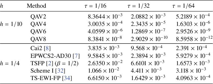
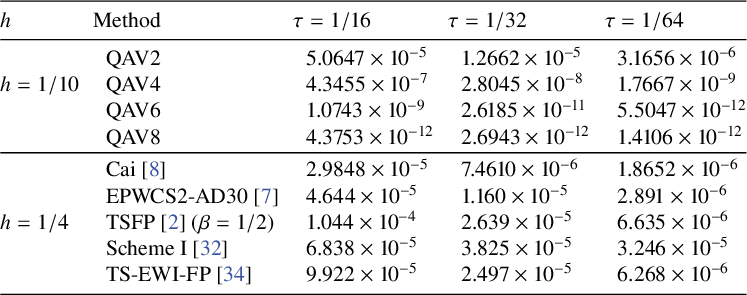
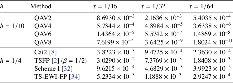
. Tables 1–3 present the
 $L_{\infty }^{n}$
errors of the solutions obtained by the QAV2, QAV4, QAV6, QAV8 and methods in the references. It is clearly seen that the proposed second-order QAV scheme QAV2 is more accurate than EPWCS2-AD30 [Reference Cai, Chen and Yang7], TSFP [Reference Bai and Wang2] and Scheme I [Reference Liao and Zhang32], and are comparative to that of Cai et al. [Reference Cai, Yang and Zhang8] and TS-EWI-PP [Reference Liao, Zhang and Wang34]. The scheme QAV8 provides the most accurate solution.
The
 $L_{\infty }^{n}$
solution errors for Example 5.1,
 $T=1$
and
 $L_{\infty }^{n}=L_{\infty }^{u}+L_{\infty }^{v}$
.

The
 $L_{\infty }^{n}$
solution errors for Example 5.2,
 $T=1$
and
 $L_{\infty }^{n}=L_{\infty }^{u}+L_{\infty }^{v}$
.

The
 $L_{\infty }^{n}$
solution errors for Example 5.3,
 $T=1$
and
 $L_{\infty }^{n}=L_{\infty }^{u}+L_{\infty }^{v}$
.

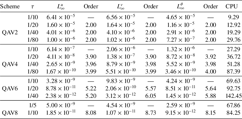
Second, to test the convergence rates of the proposed methods, we choose a relatively large calculation interval
 $[-200,200]$
. To test the convergence rates in the temporal direction, we take a relatively small spatial step
 $h=1/4$
such that the error from the spatial direction is negligible. The temporal steps are chosen as
 $\tau =1/10,1/20,1/40,1/80$
. The maximum errors and convergence rates corresponding to u, v and
 $\phi $
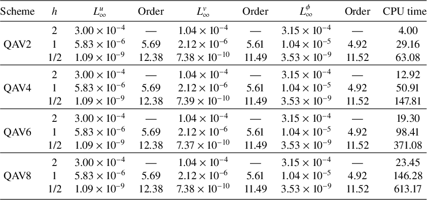
, and computational costs are presented in Table 4. It can be clearly seen that the accuracy of QAV2, QAV4, QAV6, QAV8 in the time direction can reach second-order, fourth-order, sixth-order and eighth-order, respectively. In addition, because the proposed methods are fully implicit, the QAV6 and QAV8 needs larger CPU time than the QAV2, QAV4. However, to test the numerical error in the spatial direction, we take a small time step
 $\tau =10^{-5}$
such that the error from the temporal direction is negligible. The results are presented in Table 5. It is clearly seen that the proposed schemes can reach spectral accuracy in the spatial direction.
Temporal errors and convergence order of the proposed schemes,
 $h=1/4$
,
 $T=1$
.

Temporal errors and convergence order of the proposed schemes,
 $\tau =0.00001$
,
 $T=0.01$
.

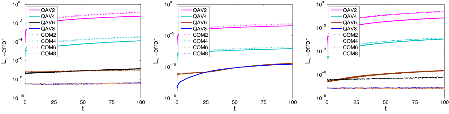
At last, to compare the proposed QAV methods with traditional composition R-K type methods (see [Reference de Frutos and Sanz-Serna10, Reference Kalogiratou, Monovasilis and Simos30, Reference Suzuki and Umeno43] for more details) and to measure the long-time computational power of our methods, we simulate Examples 5.1–5.3 over the computational domain
 $[-100,200]$
and the simulations are done up to time
 $t=100$
. The spatial step and temporal step are chosen as
 $h=1/4$
,
 $\tau =1/40$
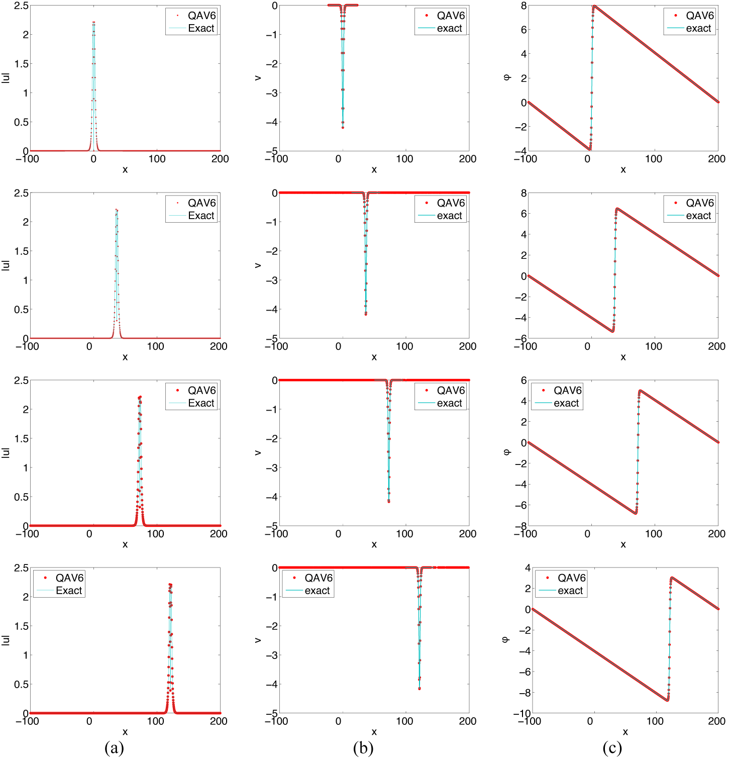
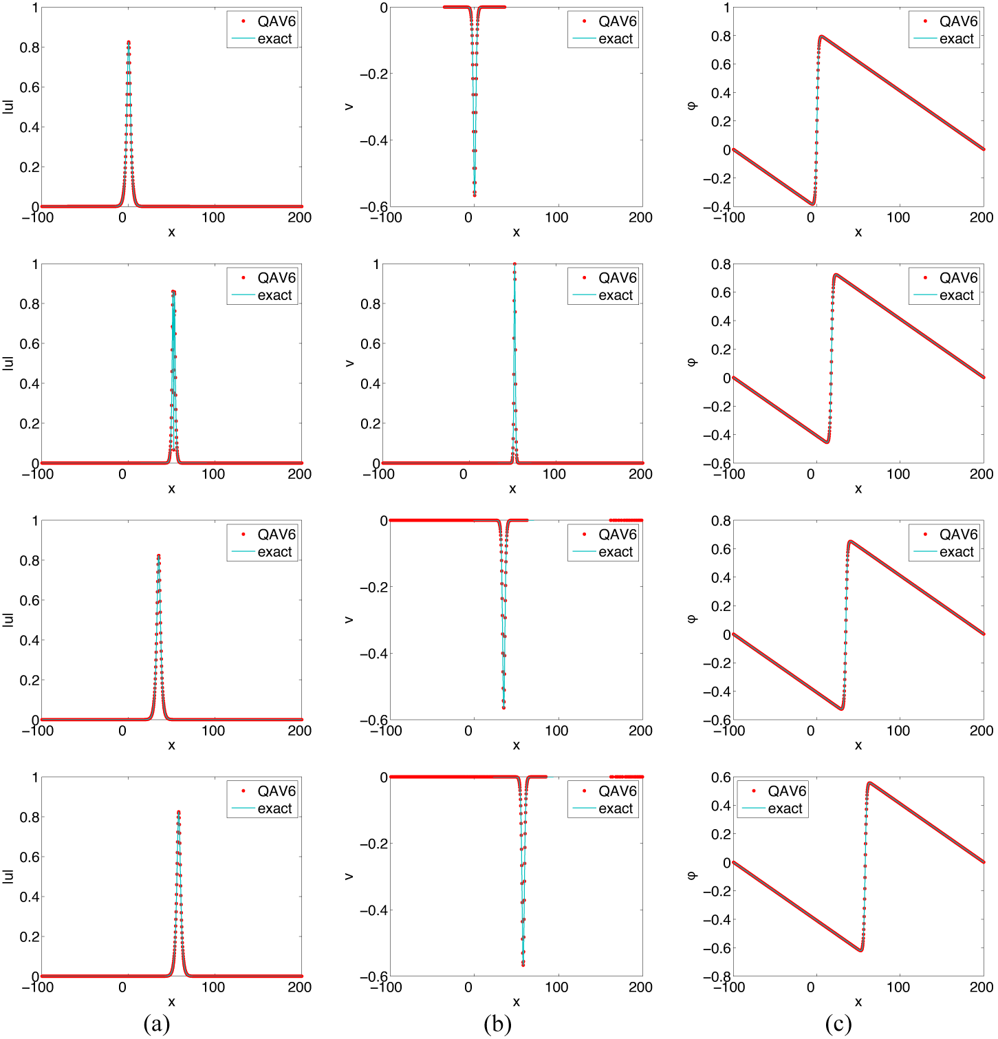
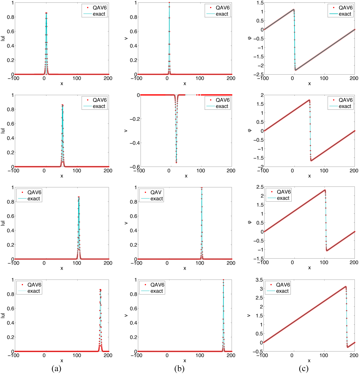
, and other parameters are identical to Examples 5.1–5.3. Plots of the exact and numerical solutions obtained by QAV6 are sketched in Figures 1–3, respectively. It is clearly seen that the exact solutions coincide exactly with the numerical solutions. The variation of the
 $L_{\infty }$
errors of the proposed QAV methods and the conventional methods are presented in Figure 4. We can see that the
 $L_{\infty }$
errors of QAV2 and QAV4 are significantly smaller than those of COM2 and COM4, respectively.
Plots of the numerical solutions of QAV6 at
 $t=0$
(top row),
 $t=30$
(the second row),
 $t=60$
(the third row) and
 $t=100$
(bottom row) in Example 5.1.

Plots of the numerical solutions of QAV6 at
 $t=0$
(top),
 $t=30$
(the second row),
 $t=60$
(the third row) and
 $t=100$
(bottom) in Example 5.2.

Plots of the numerical solutions of QAV6 at
 $t=0$
(top),
 $t=30$
(the second row),
 $t=60$
(the third row) and
 $t=100$
(bottom) in Example 5.3.


To examine the conservative properties of the proposed schemes, we define relative errors of discrete invariants by the following formulae:
 $$ \begin{align*} R_{I_{i}}^{n}=\frac{|I_{i}^{n}-I_{i}^{0}|}{|I_{1}^{0}|},\quad (i=1,2)\quad \text{and} \quad R_{E}^{n}=\frac{|E^{n}-E^{0}|}{|E^{0}|}. \end{align*} $$
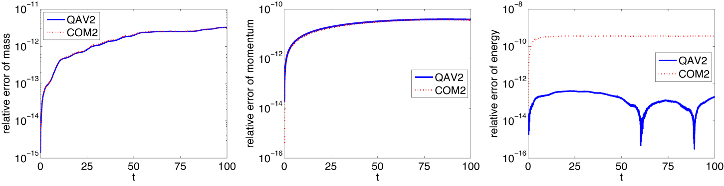
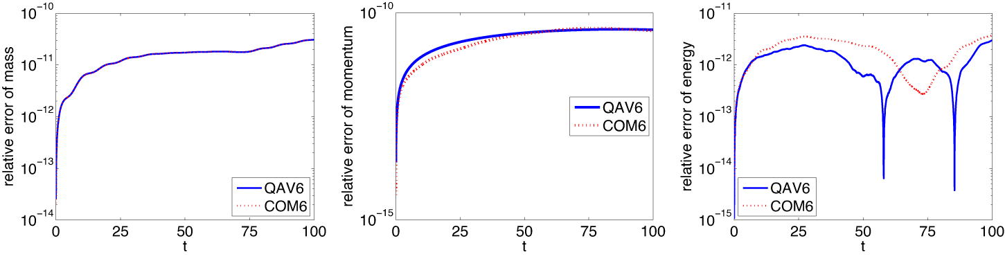
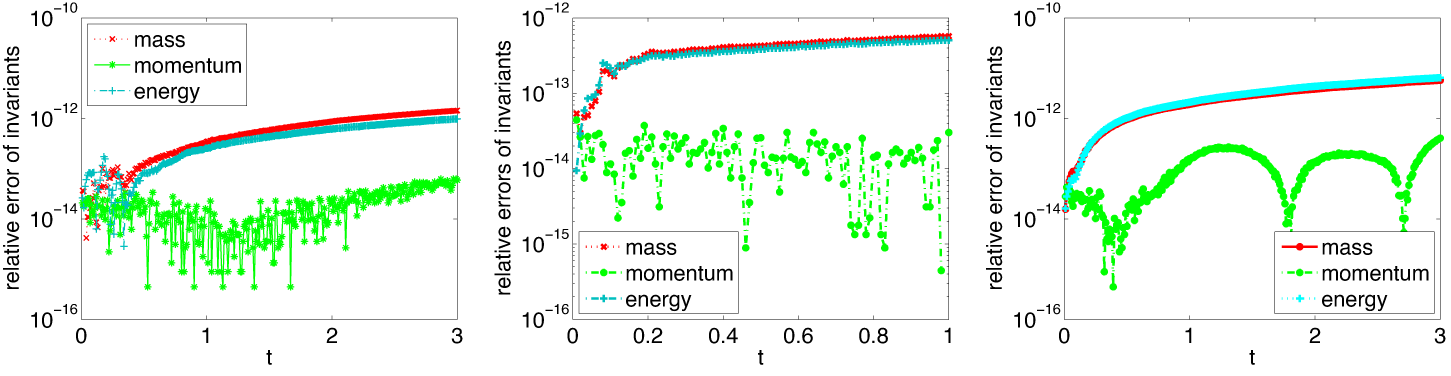
To further compare the proposed schemes with the traditional methods, we have computed the global invariants and the relative errors of them. The results are displayed in Figures 5 and 6. It is clearly seen that the traditional scheme COM2 cannot conserve the discrete energy, but the energy error computed by the COM6 with high accuracy is also small. In contrast, the proposed schemes all can warrant the conservation of the discrete invariants. These results further illustrate the effectiveness of our schemes.
The time evolution of the relative errors of discrete invariants in Example 5.2. Left,
 $I_{1}^{n}$
; middle,
 $I_{2}^{n}$
; right,
 $E^{n}$
.

The time evolution of the relative errors of discrete invariants in Example 5.2. Left,
 $I_{1}^{n}$
; middle,
 $I_{2}^{n}$
; right,
 $E^{n}$
.

5.2. Two-dimensional Schrödinger–Boussinesq system
Example 5.4 In this example, to test the accuracy of the proposed methods, we consider the following nonhomogeneous two-dimensional problems [Reference He and Chen28]:
 $$ \begin{align} \begin{cases} iu_{t}+\mu\Delta u=\omega uv+a(x,y,t),\\ v_{t}=\Delta \phi+b(x,y,t),\\ \phi_{t}=v-\varepsilon\Delta v+\theta v^{2}+\beta|u|^{2}+c(x,y,t),\\ \end{cases} \end{align} $$
where
 $\mu =\omega =\varepsilon =\theta =\beta =1$
,
 $\Omega =[0,2\pi ]\times [0,2\pi ]$
, and the computation time is done up to time
 $t=1$
. The system (5.1) has the following exact solutions:
 $$ \begin{align*} \begin{cases} u(x,y,t)=\sin{x}\sin{y}\exp({-it}),\\ v(x,y,t)=\sin{x}\sin{y}\exp({t}),\\ \phi(x,y,t)=\sin^{2}{x}\sin^{2}{y}\exp({2t}).\\ \end{cases} \end{align*} $$
The initial conditions and source terms can be determined by the system (5.1) and the above exact solutions. The proposed schemes and algorithms can be easily adapted to solve the above system (5.1) by adding source terms
 $(a_{ij}^{n})$
,
 $(b_{ij}^{n})$
and
 $(c_{ij}^{n})$
to the scheme (3.3).
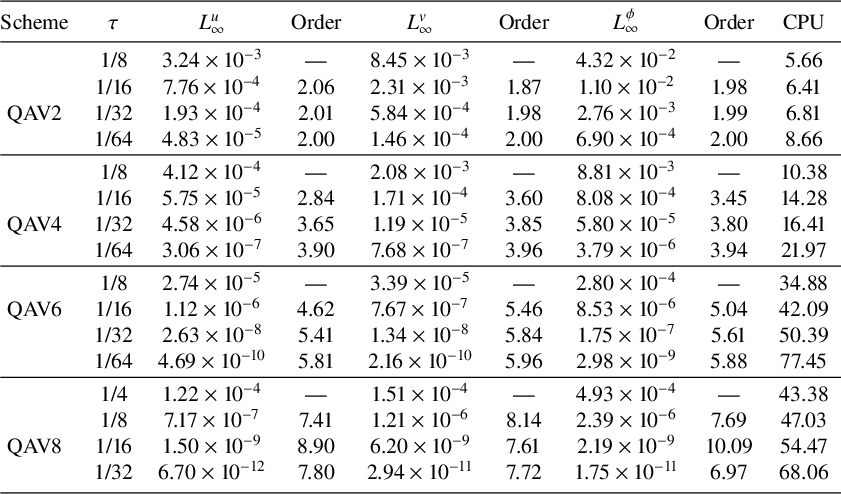
To test the convergence rates in the temporal direction, we first take a relatively small spatial step
 $h_{x}=h_{y}=\pi /20$
such that the error from the spatial direction is negligible. The temporal steps are chosen as
 $\tau =1/8, 1/16, 1/32, 1/64$
. The maximum errors and convergence rates corresponding to u, v and
 $\phi $
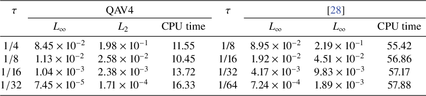
, and computational costs are presented in Table 6. It can be clearly seen that the accuracy of QAV2, QAV4, QAV6 and QAV8 in the time direction can reach second-order, fourth-order, sixth-order and eighth-order, respectively. In addition, because the proposed methods are fully implicit, QAV6 and QAV8 need larger CPU time than QAV2 and QAV4. However, to test the numerical error in the spatial direction, we take a small time step
 $\tau =10^{-5}$
such that the error from the temporal direction is negligible. The spatial steps are chosen as
 $h_{x}=h_{y}=\pi /2,\pi /4$
. The results of QAV2 are presented in Table 7. As shown in Table 7, the numerical errors reach machine precision when
 $h_{x}=h_{y}=\pi /2$
. Thus, the convergence rates of the proposed methods in the spatial direction are not trivially calculated. Nevertheless, the above results also show that the proposed schemes can achieve spectral accuracy in the spatial direction to a certain extent.
Temporal errors and convergence order of the proposed schemes,
 $h=\pi /20$
,
 $T=1$
.

Temporal errors and convergence order of the proposed schemes,
 $\tau =0.00001$
,
 $T=0.01$
.

However, to compare the proposed schemes with the linearly implicit compact finite difference method in [Reference He and Chen28], we choose spatial steps
 $h_{x}=h_{y}=\pi /20$
and the temporal steps
 $\tau =1/4,1/8,1/16,1/32$
, while the method in [Reference He and Chen28] takes
 $\tau =1/8,1/16,1/32,1/64$
. The results are presented in Table 8. It can be clearly seen that QAV4 is more efficient and has higher accuracy than the method in [Reference He and Chen28]. This further illustrates that the advantage of the high-order temporal methods, that is, it can produce more accurate results with larger time steps.
Comparison of errors and CPU time with
 $h=\pi /20$
and different time steps
 $\tau $
for Example 5.4 at
 $T=1$
.

Example 5.5 Here, we will consider a two-dimensional Schrödinger–Boussinesq system with
 $f(v)=v^{2}$
,
 $\mu =\varepsilon =\beta =1/2$
,
 $\omega =3/2$
and
 $\theta =2$
. The initial data are taken as
 $$ \begin{align*}\begin{aligned} &u_{0}(x,y)=\frac{2}{e^{(x^{2}+2y^{2})}+e^{-(x^{2}+2y^{2})}}e^{5i/\cosh(\sqrt{4x^{2}+y^{2}})},\quad x,y\in\Omega\\ &v_{0}(x,y)=e^{-(x^{2}+y^{2})},\quad \phi_{0}(x,y)=\frac{1}{2}e^{-(x^{2}+y^{2})},\quad x,y\in\Omega,\\ \end{aligned} \end{align*} $$
where
 $\Omega =[-20,20]\times [-20,20]$
. In the following, we will use the sixth-order QAV scheme QAV6 to solve the Schrödinger–Boussinesq system. Here,
 $\tau =0.01$
,
 $h_{x}=h_{y}=1/2$
, and the simulation is done up to time
 $T=3$
.
Figure 7 displays the surface plots of
 $|u|$
(left column), v (middle column) and
 $\phi $
(right column) at different times. In the left figure, we see that the initial soliton gradually collapses and expands in the opposite direction as time evolves, and some smaller solitons are formed at last. The middle graph for v shows that the initial soliton also shrinks as time progresses, a hole is formed inside the soliton, a spike is observed beneath the horizontal plane and a continuous radiation wave is observed on the horizontal plane. The figure for
 $\phi $
also displays similar variations, but no spike is observed.
Example 5.6 In this example, we will consider the Zakharov system [Reference Cai, Chen and Yang7], which is a special case of the Schrödinger–Boussinesq system when
 $f(v)=0$
,
 $\varepsilon =0$
,
 $\mu =1$
and
 $\omega =\beta =1/10$
. The initial conditions and computational domain are identical to Example 5.5. Here, for comparison, we still use QAV6 to solve this problem. The parameters
 $\tau =0.01$
,
 $h_{x}=h_{y}=1/2$
, and the simulation is done up to time
 $T=1$
. The surface plots of
 $|u|$
, v and
 $\phi $
are displayed in Figure 8. From the surface plot of
 $|u|$
, one see that the evolution of the soliton is similar to Example 5.5. The behaviour of v is also analogous to Example 5.3, but no radiation waves appears. In the right plots, also no radiation waves appear.
Surface plots of
 $|u|$
, v and
 $\phi $
at
 $t=0$
(top),
 $0.5$
(the second row),
 $1$
(the third row),
 $2$
(the fourth row) and
 $3$
(bottom).

Surface plots of
 $|u|$
, v, and
 $\phi $
at
 $t=0$
(top),
 $0.5$
(middle) and
 $1$
(bottom).

Example 5.7 In this example, we will consider the numerical solutions of the following Schrödinger–Boussinesq system [Reference Deng and Wu11]:
 $$ \begin{align} \begin{cases} iu_{t}+\mu\Delta u+\sigma |u|^{2}u-\omega uv=0,\quad (\mathbf{x},t)\in \Omega\times [0,T],\\ v_{t}-\Delta \phi=0,\quad (\mathbf{x},t)\in \Omega\times [0,T],\\ \phi_{t}-v+\varepsilon\Delta v-g(v)-\beta |u|^{2}=0,\quad (\mathbf{x},t)\in \Omega\times [0,T],\\ u(\mathbf{x},0)=u_{0}(\mathbf{x}),\quad \mathbf{x}\in\Omega\subset \Omega,\\ \end{cases} \end{align} $$
Under the periodic boundary conditions, (5.2) satisfies the following discrete invariants:
 $$ \begin{align*} &\Psi_{1}^{n+1}-(V^{n+1})^{2}=\Psi_{1}^{n}-(V^{n})^{2},\quad n=0,1,\ldots,\\ &\Psi_{2}^{n+1}-(P^{n+1})^{2}-(Q^{n+1})^{2}=\Psi_{2}^{n}-(P^{n})^{2}-(Q^{n})^{2},\quad n=0,1,\ldots,\\ &I_{1h}^{n+1}=I_{1h}^{n},\quad I_{1h}^{n}=(|U^{n}|^{2},\mathbf{1})_{h}\quad n=0,1,\ldots,\\ &I_{2h}^{n+1}=I_{2h}^{n},\quad I_{2h}^{n}=(V^{n},\mathbf{1})_{h}\quad n=0,1,\ldots,\\ &\widetilde{E}_{h}^{n+1}=\widetilde{E}_{h}^{n},\\ &\widetilde{E}_{h}^{n}=(V^{n},V^{n})_{h}-(\mathcal{D}\Phi^{n},\Phi^{n})_{h}- \frac{2\mu\beta}{\omega}(\mathcal{D}(P^{n}+Q^{n}),P^{n}+Q^{n})_{h}\\ &\qquad-\alpha(\mathcal{D}V^{n},V^{n})_{h}+\frac{2}{3}\theta (V^{n},\Psi_{1}^{n})_{h}+2\omega(V^{n},\Psi_{2}^{n})_{h}-\frac{\beta\sigma}{\omega} (\Psi_{2}^{n},\Psi_{2}^{n})_{h},\quad n=0,1,\ldots. \end{align*} $$
Here, we take
 $f(v)=v^{2}$
,
 $\mu =\varepsilon =\theta =1$
,
 $\omega =\beta =1/10$
. The parameters
 $\tau =0.01$
,
 $h_{x}=h_{y}=1/2$
, and the computation is done up to time
 $t=3$
. The initial data are similar to Example 5.5, and the computation domain is chosen as
 $[-5,5]\times [-5,5]$
. Figure 9 displays the surface plots of
 $|u|$
, v and
 $\phi $
at different moments. From the surface plot of
 $|u|$
(left picture), we see that the initial soliton expands more broadly and evolves into more small solitary waves after introducing a nonlinear term
 $\sigma |u|^{2}u$
. Numerical solutions V and
 $\Phi $
also spread around as time evolves, which is similar to Example 5.5.
Surface plots of
 $|u|$
, v and
 $\phi $
at
 $t=0$
(top),
 $0.5$
(the second row),
 $1$
(the third row),
 $2$
(the fourth row) and
 $3$
(bottom).

The relative errors of invariants for Examples 5.5–5.7 are displayed in Figure 10. It is clearly seen that the QAV6 can conserve the discrete invariants very well, which further illuminates the effectiveness of the proposed schemes.

6. Conclusions
In this paper, based on the MQAV method, we develop a family of fully decoupled arbitrarily high-order energy-preserving schemes to solve the coupled Schrödinger– Boussinesq system. Rigorous analyses show that the proposed schemes can preserve the original energy under some consistent initial conditions. Numerical results show that the proposed schemes can reach spectral accuracy in the spatial direction and arbitrarily high-order accuracy in the temporal direction. Furthermore, the schemes are efficient and also precisely conserve the discrete invariants. It further illustrates the numerical algorithms are effective and can be extended to other Hamiltonian partial differential equations.
Acknowledgements
This work is partially supported by the National Natural Science Foundation of China (Grant Nos. 11861047, 12461070, 11971241), Natural Science Foundation of Fujian Province (Grant Nos. 2019J01831,2023J011058) and Wuyi University teacher–student cooperation scientific research team project (Grant Nos. 2020-SSTD-003, 2020-ZXHZ-001). The authors are very grateful to reviewers for carefully reading this paper, and for their comments and suggestions.