

Implications
Live weights at different growth stages are frequently used as selection criteria for carcass weight at slaughter. In this study, non-linear recursive models were applied to study the genetic and phenotypic relationship between weight traits during growth. The results imply that the predictive ability of the performance of future growth is low if it is only based on records of early weights. The usefulness of slaughterhouse records in beef cattle breeding evaluation is confirmed.
Introduction
The economic efficiency of beef cattle production is strongly linked with carcass weight at slaughter (Golden et al., Reference Golden, Garrick, Newman and Enns1998; MacNeil Reference MacNeil2003; Bouquet et al., Reference Bouquet, Fouilloux, Renand and Phocas2010). In many breeding programs, carcass weight is included in selection goals as one of the most relevant traits. However, phenotypic records for this trait are not available for the potential candidates for selection. Weight records at different growth stages are therefore widely used as selection criteria on the basis that there is a strong and positive genetic correlation between early weights and weight at slaughter (Meyer et al., Reference Meyer, Carrick and Donnelly1993; Altarriba et al., Reference Altarriba, Yagüe, Moreno and Varona2009; Bouquet et al., Reference Bouquet, Fouilloux, Renand and Phocas2010). The breeding scheme established by the Pirenaica breeders association (Confederación Nacional de Asociaciones de Vacuno Pirenaica (CONASPI)) uses weight records between 110 and 310 days of age as predictors for future weight at slaughter (Altarriba et al., Reference Altarriba, García-Cortés, Moreno and Varona1996; Varona et al., Reference Varona, Moreno, García Cortés and Altarriba1997).
Nevertheless, the potential presence of compensatory growth (Smith and Hodnett, Reference Smith and Hodnett1962; Blanco et al., Reference Blanco, Villalba, Ripoll, Sauerwein and Casasus2009; Neto et al., Reference Neto, Bezerra, Medeiros, Ferreira, Pimenta, Candido and Oliveira2011) may reduce the efficiency of the use of early weights as a predictor of weight at slaughter. In a previous study with the same population (González-Rodríguez et al., Reference González-Rodríguez, Altarriba, Moreno and Varona2011), it was shown that genetic correlations between weight gain and weights recorded earlier in life were very low and that residual correlations between them may even be negative. These results imply the presence of compensatory growth in the Pirenaica beef cattle population, something that has also been suggested by Blanco et al. (Reference Blanco, Villalba, Ripoll, Sauerwein and Casasus2009).
From an alternative perspective, recursive models (Gianola and Sorensen, Reference Gianola and Sorensen2004) may be a valuable approach for the analysis of sequential traits as successive weights during growth. As argued by Valente et al. (Reference Valente, Rosa, Gianola, Wu and Weigel2013), recursive models allow the estimation of the genetic effects acting directly on one trait, without the influence of other traits. This approach is able to analyze weights without the phenotypic influence of a trait measured in a previous stage. Further, non-linear versions of recursive models (López de Maturana et al., Reference López de Maturana, Wu, Gianola, Weigel and Rosa2009; Ibáñez-Escriche et al., Reference Ibáñez-Escriche, López de Maturana, Noguera and Varona2010; Varona and Sorensen, Reference Varona and Sorensen2014) could help to describe the kind of relationship between weights that may appear as compensatory growth.
The aim of this study is to explore the possibilities of recursive models for the analysis of successive weights in Pirenaica beef cattle. The objective is to describe the genetic determinism of the beef cattle growth process from an alternative point of view.
Material and methods
Data
The data sets used in this study were provided by two organizations: (i) the Pirenaica Breeders Association (CONASPI) contributed 173 719 live weights records and a pedigree of 205307 cases from 1989 to 2009; (ii) the System of Identification and Traceability provided 28 724 carcass weight records recorded at slaughterhouses from 2003 to 2009. Live weights registered between 80 and 160 days of life were used to adjust the phenotypes of weight at 120 days (W120) and records between 170 and 250 were used to adjust weight at 210 days (W210). Both traits were adjusted using sex-specific average daily gain in the population and the closer available weight, following the recommendations of the Beef Improvement Federation (2010). The same strategy was used with carcass weights between 250 and 480 days of age to predict carcass weight at 365 days (CW365).
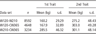
Three subsets of data composed by records from individuals with available phenotypic information for each pair of traits were then created. These subsets consisted of 8592, 4648 and 3234 records for W120-W210, W120-CW365 and W210-CW365, respectively. Means and phenotypic standard deviations are presented in Table 1. In addition, an operational pedigree composed of 56 323 individuals generated from the genealogical information provided by CONASPI with the software RenumF90 (Misztal, Reference Misztal2012) was established.
Means and phenotypic standard deviations for the analysed traits

s.d.=standard deviation; W120=weight at 120 days of age; W210=weight at 210 days; CW365=cold carcass weight.
Model of analysis
Each subset of data was analyzed using a bivariate recursive model for traits taken in pairs (W120-W210, W120-CW365 and W210-CW365). For traits registered early in life or independent (
 $$I$$
, as W120 or W210), the following model was assumed:
 $${\bf y}_{I} ={\bf X}_{I} {\bf b}_{I} {\plus}{\bf Z}_{I} {\bf u}_{I} {\plus}{\bf e}_{I} $$
where y
I
is the vector of phenotypic records, b
I
is the vector of systematic effect (year-season of birth, sex and herd), u
I
is the vector of additive genetic effects and
 $${\bf e}_{I} $$
is the vector of residual effects. Further, X
I
and Z
I
are incidence matrices that link phenotypic records with systematic and additive genetic effects.
Traits measured latterly or dependent (
 $$D$$
, as W210 or CW365) were analyzed with four alternative models:
 $${\bf y}_{D} =\lambda _{{DI}} {\bf s}_{I} {\plus}{\bf X}_{D} {\bf b}_{D} {\plus}{\bf Z}_{D} {\bf u}_{D} {\plus}{\bf e}_{D} $$
 $${\bf y}_{D} =\lambda _{{DI}} {\bf s}_{I} {\plus}\lambda _{{DI}}^{'} {\bf t}_{I} {\plus}{\bf X}_{D} {\bf b}_{D} {\plus}{\bf Z}_{D} {\bf u}_{D} {\plus}{\bf e}_{D} $$
 $${\bf y}_{D} =\lambda _{{DI}} {\bf s}_{I} {\plus}\lambda _{{DI}}^{'} {\bf t}_{I} {\plus}\lambda _{{DI}}^{{''}} {\bf r}_{I} {\plus}{\bf X}_{D} {\bf b}_{D} {\plus}{\bf Z}_{D} {\bf u}_{D} {\plus}{\bf e}_{D} $$
 $${\bf y}_{D} =\lambda _{{DI}} {\bf s}_{I} {\plus}\lambda _{{DI}}^{'} {\bf t}_{I} {\plus}\lambda _{{DI}}^{{''}} {\bf r}_{I} {\plus}\lambda _{{DI}}^{{'''}} {\bf d}_{I} {\plus}{\bf X}_{D} {\bf b}_{D} {\plus}{\bf Z}_{D} {\bf u}_{D} {\plus}{\bf e}_{D} $$
where y
D
is the vector of phenotypic records for 2nd or dependent traits (W210 and CW365),
 $$\lambda _{{DI}} ,\lambda _{{DI}}^{'} ,\lambda _{{DI}}^{{''}} \,\,{\rm and}\,\,\lambda _{{DI}}^{{'''}} $$
are the recursive parameters that relate the phenotypic records with the vectors s
I
, t
I
, r
I
and d
I
, whose elements are
 $$s_{{Ij}} =\left\{ {y_{{Ij}} \,{\minus}\,\bar{y}_{I} } \right\}$$
 $$t_{{Ij}} =\left\{ {{{\left( {y_{{Ij}} \,{\minus}\,\bar{y}_{I} } \right)^{2} } \over {100}}} \right\}$$
 $$r_{{Ij}} =\left\{ {{{\left( {y_{{Ij}} \,{\minus}\,\bar{y}_{I} } \right)^{3} } \over {10\:000}}} \right\}$$
 $$d_{{Ij}} =\left\{ {{{\left( {y_{{Ij}} \,{\minus}\,\bar{y}_{I} } \right)^{4} } \over {1\:000000}}} \right\}$$
where y
Ij
is the phenotypic record for the jth individual and
 $$\overline{y} _{I} $$
is the average performance for the independent trait.
Additionally, b D is a vector of systematic effects (year-season of birth, sex, herd and also slaughterhouse for CW365), u D is the vector of additive genetic effects and e D is the vector of residual effects. X D and Z D are incidence matrices that relate phenotypic records with systematic and additive genetic effects, respectively.
The statistical analysis was performed using a Bayesian approach. For reasons of simplicity, only the joint posterior distribution for model 4 is described in detail:
 $$\eqalignno{ & p\left( {\left. {{\bf b}_{I} ,{\bf b}_{D} ,{\bf u}_{I} ,{\bf u}_{D} ,{\bf G},\lambda _{{DI}} ,\lambda _{{DI}}^{'} ,\lambda _{{DI}}^{{''}} ,\lambda _{{DI}}^{{'''}} ,\sigma _{{EI}}^{2} ,\sigma _{{ED}}^{2} } \right|{\bf y}_{I} ,{\bf y}_{D} } \right)\propto \cr & p\left( {\left. {{\bf y}_{I} } \right|{\bf b}_{I} ,{\bf u}_{I} ,\sigma _{{EI}}^{2} } \right)p\left( {\left. {{\bf y}_{D} } \right|{\bf b}_{D} ,{\bf u}_{D} ,{\bf y}_{I} ,\lambda _{{DI}} ,\lambda _{{DI}}^{'} ,\lambda _{{DI}}^{{''}} ,\lambda _{{DI}}^{{'''}} ,\sigma _{{ED}}^{2} } \right) \cr & p\left( {{\bf b}_{I} } \right)p\left( {{\bf b}_{D} } \right)p\left( {\left. {{\bf u}_{I} ,{\bf u}_{D} } \right|{\bf G}} \right)p\left( {\bf G} \right)p\left( {\lambda _{{DI}} } \right)p\left( {\lambda _{{DI}}^{'} } \right)p\left( {\lambda _{{DI}}^{{''}} } \right) \cr \qquad \qquad \qquad p\left( {\lambda _{{DI}}^{{'''}} } \right)p\left( {\sigma _{{EI}}^{2} } \right)p\left( {\sigma _{{ED}}^{2} } \right) $$
where G is the additive genetic (co)variance matrix,
 $$\sigma _{{EI}}^{2} $$
and
 $$\sigma _{{ED}}^{2} $$
are the residual variances for the independent and the dependent traits, respectively, and
 $$p\left( {\left. {{\bf y}_{I} } \right|{\bf b}_{I} ,{\bf u}_{I} ,\sigma _{{EI}}^{2} } \right)\propto\prod\limits_{j=1}^n {{1 \over {\left( {2\pi \sigma _{{EI}}^{2} } \right)^{{{1 \over 2}}} }}\exp \left[ {{\minus}{{\left( {y_{{Ij}} \,{\minus}\,{\bf x}_{{Ij}}^{'} {\bf b}_{I} \,{\minus}\,{\bf z}_{{Ij}}^{'} {\bf u}_{I} } \right)^{2} } \over {2\sigma _{{EI}}^{2} }}} \right]} $$
where
 ${\rm x}_{{I\,j}}^{'} $
and
 ${\rm z}_{{I\,j}}^{'} $
are vectors of the incidence matrices that correspond to the jth individual for the independent trait, n is the number of records, and
 $$\eqalignno{ & p\left( {\left. {{\bf y}_{D} } \right|{\bf b}_{D} ,{\bf u}_{D} ,{\bf y}_{I} ,\lambda _{{DI}} ,\lambda _{{DI}}^{'} ,\lambda _{{DI}}^{{''}} ,\lambda _{{DI}}^{{'''}} ,\sigma _{{ED}}^{2} } \right) \hskip 3pt\propto \hskip 3pt \prod\limits_{j=1}^n {{1 \over {\left( {2\pi \sigma _{{ED}}^{2} } \right)^{{{1 \over 2}}} }}} \cr \ \; \exp \left[ {{\minus}{{\left( {{\rm y}_{{Dj}} {\minus}{\bf x}_{{Dj}}^{'} {\bf b}_{D} {\minus}{\bf z}_{{Dj}}^{'} {\bf u}_{D} {\minus}\lambda _{{DI}} {\rm s}_{{Ij}} {\minus}\lambda _{{DI}}^{'} {\rm t}_{{Ij}} {\minus}\lambda _{{DI}}^{{''}} {\rm r}_{{Ij}} {\minus}\lambda _{{DI}}^{{'''}} {\rm d}_{{Ij}} } \right)^{2} } \over {2\sigma _{{ED}}^{2} }}} \right]} $$
where
 ${\rm x}_{{D\,i}}^{'} $
and
 ${\rm z}_{{Di}}^{'} $
are vectors of incidence matrices corresponding at jth individual for the dependent trait.
The prior distribution for the additive breeding values was the following multivariate Gaussian distribution:
 $$\eqalign {p\left( {\left. {{\bf u}_{I} ,{\bf u}_{G} } \right|{\bf G}} \right)\propto{1 \over {\left( {2\pi } \right)^{{{n \over 2}}} \left| {{\bf A}\,\otimes\,{\bf G}} \right | ^{{{1 \over 2}}} }} \exp \left[ {{\minus}{{\left( {{\bf u}_{I} ,{\bf u}_{D} } \right)^{'} \left( {{\bf A}\,\otimes\,{\bf G}} \right)^{{{\minus}1}} \left( {{\bf u}_{I} ,{\bf u}_{D} } \right)} \over 2}} \right]$$
where A is the additive relationship matrix. The prior distributions for systematic effects, recursive parameters and variance components are assumed to be bounded uniform distributions between −10 000 and 10 000 for systematic effects and recursive parameters and between 0 and 10 000 for variance components.
The analysis was a Bayesian inference through Gibbs sampler algorithm (Gelfand et al., Reference Gelfand, Hills, Racine-Poon and Smith1990) using a modified version of program TM (Legarra et al., Reference Legarra, Varona and López de Maturana2008). For the Gibbs sampler implementation, samples from the full conditional distributions are needed. In this case, the full conditional distributions for systematic and additive genetic effects are Gaussian distributions as well as the conditional distributions of the recursive parameters. The conditional distributions for the residual variances are inverted χ 2 distributions and, finally, the conditional distribution for the additive (co)variance matrix is an inverted Wishart distribution. The Gibbs sampler was implemented with a single long chain of 525 000 iterations after a burn-in of 25 000 iterations. Convergence was checked using the Raftery and Lewis (Reference Raftery and Lewis1992) algorithm.
Comparison between models
Alternative models were compared with a leave-one-out cross-validation, an approach (Gelfand et al., Reference Gelfand, Dey and Chang1992) that is based on the prediction ability of the posterior distribution as a measure of the fit of model. We consider the data vector
 $${\rm y}'=(y_{i} ,y_{{{\rm {-}}i}} )$$
where yi is the ith datum, and y
−i is the vector of data with ith datum deleted. This procedure needs to build the posterior predictive density for each record
 $${\rm y}_{i} $$
conditioned to model M and the vector of data, but leaving out each particular record, y
−i
(Sorensen and Gianola, Reference Sorensen and Gianola2002):
 $$p\left( {\left. {y_{i} } \right|{\bf y}_{{{\minus}i}} ,M} \right)=\mathop{\int} {p\left( {\left. {y_{i} } \right|\theta ,{\bf y}_{{{\minus}i}} ,M} \right)p\left( {\left. \theta \right|{\bf y}_{{{\minus}i}} ,M} \right)d\theta } $$
where θ is the vector the parameters of the model. In example, the vector of parameters for model 4 is
 $$\theta =\left\{ {{\bf b}_{I} ,{\bf b}_{D} ,{\bf u}_{I} ,{\bf u}_{D} ,{\bf G},\lambda _{{DI}} ,\lambda _{{DI}}^{'} ,\lambda _{{DI}}^{{''}} ,\lambda _{{DI}}^{{'''}} ,\sigma _{{EI}}^{2} ,\sigma _{{ED}}^{2} } \right\}$$
The values of the posterior predictive density
 $$p\left( {\left. {y_{i} } \right|{\bf y}_{{{\minus}i}} ,M} \right)$$
, also known as CPOi (Conditional Predictive Ordinate), can be used as a measure of the fit for the ith specific record and
 $${\rm CPO}_{M} =\prod\limits_{i=1}^n {p\left( {\left. {y_{i} } \right|{\bf y}_{{{\minus}i}} ,M} \right)} $$
is a direct measure of the global fit of all records (Ibáñez-Escriche et al., Reference Ibáñez-Escriche, Varona, Casellas, Quintanilla and Noguera2009). A lower CPOM indicates a lack of fitness of the model M. Under a Markov Chain Monte Carlo scheme, such as the Gibbs sampler, these values are approximated through
 $$\hat{p}\left( {\left. {{\rm y}_{i} } \right|{\bf y}_{{{\minus}i}} ,M} \right)={1 \over {\mathop{\sum}\limits_{j=1}^{iter} {{1 \over {p\left( {\left. {{\rm y}_{i} } \right|\theta _{j} ,\,{\bf y}_{{{\minus }i}} ,\,M} \right)}}} }}$$
where
 $p(\left. {y_{i} } \right|\theta _{j} ,{\rm y}_{{{-}i}} ,M)$
is the predictive density of ith data at the jth iteration of the Gibbs sampler given the current sample of the vector of parameters (θ
j
), and iter is total number of iterations after convergence. As suggested by Geisser (Reference Geisser1993), the Logarithm of CPO for model M (log CPOM) can be calculated through
 $$\log {\rm CPO}_{M} =\mathop{\sum}\limits_{i=1}^n {\log \left( {\hat{p}\left( {\left. {y_{i} } \right|{\bf y}_{{{\minus}i}} ,M} \right)} \right)} $$
In this work, it was used as a diagnostic measure to evaluate the predictive ability of the model: models with highest log CPOM are understood as the models with the best predictive ability of data.
Calculation of unconditional breeding values and additive (co)variance matrix
The implementation of recursive models provides predictions of breeding values for the independent (u
I
) and the dependent trait (u
D
), but the last are conditional to the recursive relationships with the independent trait. Under the standard linear recursive models (Gianola and Sorensen, Reference Gianola and Sorensen2004; Valente et al., Reference Valente, Rosa, Gianola, Wu and Weigel2013), the breeding value for the dependent trait for the jth individual can be deconditioned (
 $${\rm u}_{{D_{j} }}^{{\asterisk}} $$
) using the following expression:
 $$u_{{D_{j} }}^{{\asterisk}} =u_{{Dj}} {\plus}\lambda _{{DI}} u_{{Ij}} $$
However, under the proposed non-linear recursive model, the deconditioning procedure becomes more complex when higher order polynomials are assumed. Nevertheless, the dependency between both models at a given phenotype (k) for the independent trait of the jth individual can be approximated by using a 1st order Taylor expansion of the non-linear recursive function f(y Ij ):
 $$\eqalignno{ & y_{{Dj}} =f\left( {y_{{Ij}} } \right){\plus}{\bf x}_{{Dj}}^{'} {\bf b}_{D} {\plus}{\rm u}_{{Dj}} {\plus}{\rm e}_{{D_{j} }} \,\approx\, \cr & f\left( {y_{{Ij}} =k} \right){\plus}{{f^{'} \left( {y_{{Ij}} =k} \right)} \over {1 !\,}}\left( {y_{{I_{j} }} {\minus}k} \right){\plus}{\bf x}_{{Dj}}^{'} {\bf b}_{D} {\plus}{\rm u}_{{Dj}} {\plus}{\rm e}_{{Dj}} $$
as
 $$y_{{Ij}} ={\bf x}_{{Ij}}^{'} {\bf b}_{I} {\plus}u_{{Ij}} {\plus}e_{{Ij_{j} }} $$
The unconditional breeding value for the jth individual and for the dependent trait (
 $$u_{{Dj}}^{{\asterisk}} $$
) is approximately
 $$u_{{Dj}}^{{\asterisk}} =\omega _{k} u_{{Ij}} {\plus}u_{{Dj}} $$
being
 $$\omega _{k} =f^{'} \left( {y_{{Ij}} =k} \right)$$
Further, under this linear approximation, the unconditional matrix of additive genetic (co)variance between traits
 $\left( {{\rm G}_{k}^{{\asterisk}} } \right)$
at the phenotypic value
 $$k$$
of the independent trait can be calculated as:
 $${\bf G}_{k}^{{\asterisk}} =\left( {{\bf I}{\minus}\Lambda _{k} } \right)^{{{\minus}1}} {\bf G}_{0} \left( {{\bf I}{\minus}\Lambda _{k} } \right)^{{{\minus}1^{'}}} $$
where
 $$\Lambda _{k} =\left[ {\matrix{ 0 & 0 \cr {\omega _{k} } & 0 \cr } } \right]$$
and
 $${\bf G}_{0} =\left[ {\matrix{ {\sigma _{{AI}}^{2} } & {\sigma _{{AID}} } \cr {\sigma _{{AID}} } & {\sigma _{{AD}}^{2} } \cr } } \right]^{'} $$
being
 $\sigma _{{AI}}^{2} $
the additive variance for the independent trait,
 $\sigma _{{AD}}^{2} $
the additive variance for the dependent trait, and
 $\sigma _{{AID}} $
the additive covariance between the independent and dependent traits. These are the parameters that provided the McMC estimation under models 1 to 4. Thus, the unconditional genetic (co)variance matrix at this phenotypic value for the independent trait is approximated as:
 $${\bf G}_{k}^{{\asterisk}} =\left[ {\matrix{ {\sigma _{{AI}}^{2} } & {\sigma _{{AI}}^{2} \omega _{k} {\plus}\sigma _{{AID}} } \cr {\sigma _{{AI}}^{2} \omega _{k} {\plus}\sigma _{{AID}} } & {\omega _{k} \left( {\sigma _{{AI}}^{2} \omega _{k} {\plus}2\sigma _{{AID}} } \right){\plus}\sigma _{{AD}}^{2} } \cr } } \right]^{'} $$
Further, the unconditional genetic correlation at the phenotypic value
 $$k$$
of the independent trait is calculated through
 $${\rm r}_{k} ={{\sigma _{{AI}}^{2} \omega _{k} {\plus}\sigma _{{AID}} } \over {\sqrt {\sigma _{{AI}}^{2} \left( {\omega _{k} \left( {\sigma _{{AI}}^{2} \omega _{k} {\plus}2\sigma _{{AID}} } \right){\plus}\sigma _{{AD}}^{2} } \right)} }}$$
In an equivalent way, for the residual variances
 $${\bf R}_{0} =\left[ {\matrix{ {\sigma _{{EI}}^{2} } & 0 \cr 0 & {\sigma _{{ED}}^{2} } \cr } } \right]^{'} $$
and
 $${\bf R}_{k}^{{\asterisk}} =\left[ {\matrix{ {\sigma _{{EI}}^{2} } & {\sigma _{{EI}}^{2} \omega _{k} } \cr {\sigma _{{EI}}^{2} \omega _{k} } & {\sigma _{{EI}}^{2} \omega _{k}^{2} {\plus}\sigma _{{ED}}^{2} } \cr } } \right]^{'} $$
Thus, the unconditional heritability at the phenotypic value k of the independent trait is calculated by:
 $$h_{k}^{2} ={{\left( {\omega _{k} \left( {\sigma _{I}^{2} \omega _{k} {\plus}2\sigma _{{ID}} } \right){\plus}\sigma _{D}^{2} } \right)} \over {\left( {\omega _{k} \left( {\sigma _{I}^{2} \omega _{k} {\plus}2\sigma _{{ID}} } \right){\plus}\sigma _{D}^{2} } \right){\plus}\sigma _{{EI}}^{2} \omega _{k}^{2} {\plus}\sigma _{{ED}}^{2} }}$$
Results and discussion
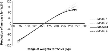
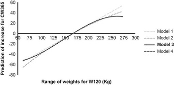
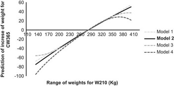
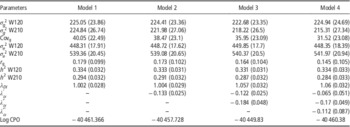
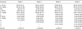
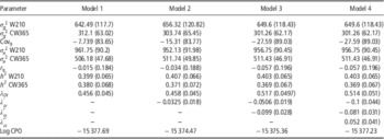
The posterior mean and s.d. for the variance and covariance components, genetic correlations, heritabilities and recursive parameters together with the respective diagnostic measures for model comparison (log CPO) are presented in Tables 2, 3 and 4, for analyses of the W120-W210, W210-CW365 and W210-CW365 data sets, respectively. The results of model comparison by log CPO indicated that the model that presented a better predictive ability included a cubic recursive function for the analyses W120-W210 and W120-CW365, while for W210-CW365 a square dependence was chosen. The selected models indicate non-linear relationships between traits as reflected in Figures 1, 2 and 3 where the recursive functions are plotted.
Prediction of the increase for W210 given W120, through the linear and non-linear recursive models. Model 1=Linear recursive model; Model 2=Non-linear recursive model with a recursive function of 2nd degree; Model 3=Non-linear recursive model with a recursive function of 3rd degree; Model 4=Non-linear recursive model with a recursive function of 4th degree.

Prediction of the increase for CW365 given W120, through linear and non-linear recursive models. Model 1=Linear recursive model; Model 2=Non-linear recursive model with a recursive function of 2nd degree; Model 3=Non-linear recursive model with a recursive function of 3rd degree; Model 4=Non-linear recursive model with a recursive function of 4th degree.

Prediction of Carcass Weight (CW365) given W210, through linear and non-linear recursive models. Model 1=Linear recursive model; Model 2=Non-linear recursive model with a recursive function of 2nd degree; Model 3=Non-linear recursive model with a recursive function of 3rd degree; Model 4=Non-linear recursive model with a recursive function of 4th degree.

Posterior mean (and s.d.) estimates of genetic and residual variance, genetic covariance, genetic correlation, heritability, parameters of recursive models and log CPO for the traits W120-W210

 $$\sigma _{\!g}^{ \ 2} $$
=genetic variance; Covg=genetic covariance;
 $$\sigma _{\!e}^{ \ 2} $$
=residual variance; r
g=genetic correlation; h
2=heritability; λ
DI
=recursive parameter;
 $$\lambda _{{_{{DI}} }}^{'} $$
=square potency;
 $$\lambda _{{_{{DI}} }}^{{''}} $$
=cube potency;
 $$\lambda _{{_{{DI}} }}^{{'''}} $$
=4th potency; W120=weight at 120 days of age; W210=weight at 210 days.
Posterior mean (and s.d.) estimates of genetic and residual variance, genetic covariance, genetic correlation, heritability, parameters of recursive models and log CPO for the traits W120-CW365

 $$\sigma _{\!g}^{\ 2} $$
=genetic variance; Covg=genetic covariance;
 $$\sigma _{\!e}^{ \ 2} $$
=residual variance; r
g=genetic correlation; h
2=heritability; λ
DI
=recursive parameter;
 $$\lambda _{{_{{DI}} }}^{'} $$
=square potency;
 $$\lambda _{{_{{DI}} }}^{{''}} $$
=cube potency;
 $$\lambda _{{_{{DI}} }}^{{'''}} $$
=4th potency; W120=weight at 120 days of age; CW365=carcass weight.
Posterior mean (and s.d.) estimates of genetic and residual variance, genetic covariance, genetic correlation, heritability, parameters of recursive models and log CPO for the traits W210-CW365

 $$\sigma _{\!g}^{ \ 2} $$
=genetic variance; Covg=genetic covariance;
 $$\sigma _{\!e}^{ \ 2} $$
=residual variance; r
g=genetic correlation; h
2=heritability; λ
DI
=recursive parameter;
 $$\lambda _{{_{{DI}} }}^{'} $$
=square potency;
 $$\lambda _{{_{{DI}} }}^{{''}} $$
=cube potency;
 $$\lambda _{{_{{DI}} }}^{{'''}} $$
=4th potency; W210=weight at 210 days of age; CW365=carcass weight.
The posterior mean estimates of the heritabilities for the independent traits or those registered early in life (W120 and W210) ranged between 0.33 and 0.43. They are in line with previous estimates from the literature obtained in the same breed (Varona et al., Reference Varona, Moreno, García Cortés and Altarriba1997; Altarriba et al., Reference Altarriba, Yagüe, Moreno and Varona2009; Varona et al., Reference Varona, Moreno and Altarriba2012), or other beef cattle populations (Ríos-Utrera and Van Vleck, Reference Ríos-Utrera and Van Vleck2004; Bouquet et al., Reference Bouquet, Fouilloux, Renand and Phocas2010). The estimates of heritabilities in the dependent traits (W210 and CW365) ranged between 0.28 (W210) to 0.38 (CW365), although they cannot be directly compared with previous estimates, because they are conditioned to the independent trait.
For the selected models, the posterior estimates of the genetic correlations between both traits ranged from −0.034 (W120-CW365) to 0.164 (W120-W210), as shown in Tables 2, 3 and 4. These genetic correlations are much smaller than previous estimates (Altarriba et al., Reference Altarriba, Yagüe, Moreno and Varona2009). However, it should be emphasized that the genetic correlations reported here have to be understood as between independent and dependent traits marginalized with respect to each other via the recursive function. In fact, the results are coherent with the authors’ previous estimates of genetic correlations between early weights and subsequent gains of weight (González-Rodríguez et al., Reference González-Rodríguez, Altarriba, Moreno and Varona2011). It should be also noted that the magnitude of the heritabilities for the dependent traits and the genetic covariance between them become smaller as the complexity of the model increases. This phenomenon implies that genetic determinism is better captured by the recursive function as the grade of the polynomial function increases, and, therefore, a lower genetic variation remains in the dependent trait.
Deconditioning breeding values and additive (co)variance matrices under a linear recursive model is an automatic task (Gianola and Sorensen, Reference Gianola and Sorensen2004; Varona et al., Reference Varona, Sorensen and Thompson2007). However, when the relationship between traits is not linear, this task becomes more complex. Some studies (López de Maturana et al., Reference López de Maturana, Wu, Gianola, Weigel and Rosa2009; Ibáñez-Escriche et al., Reference Ibáñez-Escriche, López de Maturana, Noguera and Varona2010) use a linear spline approximation to this non-linear relationship, and they generate spline specific additive (co)variance matrices associated with several parametric subspaces of the independent trait. Under the approach proposed in this study, the non-linear recursive relationship is defined in terms of polynomials up to the 4th order and specific additive (co)variance matrix for each phenotypic value are approximated by a 1st order Taylor expansion of the recursive function.
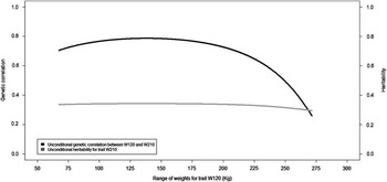
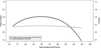
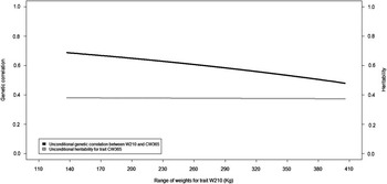
After deconditioning, the estimates of the genetic correlations can be expressed in accordance with the range of phenotypic values of the independent trait. The plots of the posterior mean estimates of these genetic correlations for the selected models are presented in Figures 4 to 6. These plots confirm the non-linear nature of the relationship between traits. The genetic correlation between W120 and W210 started at 0.7 for very low values of W120 and increased to 0.8 for weights around 140 kg. Later, and for higher values of W120, it decreased to 0.2. The genetic correlation between W120 and CW365 provided a similar plot with a maximum genetic correlation of 0.6 and a reduction of this correlation to zero for large W120 values. Finally, the genetic correlation between W210 and CW365 also decreased with the phenotypic value of W210 and ranged from 0.5 to 0.7. These estimates were substantially higher than the previous ones and much closer to the previous estimates in the same population for genetic correlation between weights at different ages (Altarriba et al., Reference Altarriba, Yagüe, Moreno and Varona2009). It should be noted that a reduction of genetic correlation for higher phenotypic values of the independent traits was present in all three data sets analyzed. This fact implies that the weight of the information on the early registered trait in the prediction of breeding values is smaller for higher phenotypic values. Further, the unconditional heritability estimates for the were more stable along the parametric space (Figures 4 to 6) and also within the range of previous estimates from the literature (Ríos-Utrera and Van Vleck, Reference Ríos-Utrera and Van Vleck2004; Altarriba et al., Reference Altarriba, Yagüe, Moreno and Varona2009; Bouquet et al., Reference Bouquet, Fouilloux, Renand and Phocas2010).
Genetic correlation between W120 and W210, and heritability of W210, for the range of values on the parametric space of W120.

Genetic correlation between W120 and CW365, and heritability of CW365, for the range of values on the parametric space of W120.

Genetic correlation between W210 and CW365, and heritability of CW365, for the range of values on the parametric space of W210.

In animal breeding, the joint analysis of several traits is usually performed through multi-trait mixed model analyses (Henderson, Reference Henderson1984). These models assume that the relationship between traits is linear and they are not able to differentiate between direct and indirect genetic effects, as those generated by causal relationships between traits (Valente et al., Reference Valente, Rosa, Gianola, Wu and Weigel2013). A linear relationship between traits implies that the increase of one unit for one trait automatically results in a modification of the other trait independent of the range of values that are considered. This assumption makes sense when analyzed traits have their phenotypic expression within a small range of phenotypic values. However, when the traits have a very wide phenotypic range of values, it seems plausible that the relationship between them is not linear. For example, Ibáñez-Escriche et al. (Reference Ibáñez-Escriche, López de Maturana, Noguera and Varona2010) analyzed the percentage of stillborns in pigs with respect to litter size and showed that there was a small relationship between lower values of litter size which increased as the litter size increased. Non-linear recursive models offer greater flexibility than recursive linear or standard multivariate mixed models as they allow the description of the non-linear relationship between traits, as previously noted by Maturana et al. (Reference López de Maturana, Wu, Gianola, Weigel and Rosa2009) and Ibáñez-Escriche et al. (Reference Ibáñez-Escriche, López de Maturana, Noguera and Varona2010). The current study puts forward an alternative version to the proposal of these authors that uses a polynomial function. It avoids the assumption or calculation of the points of change among sequential segments. Another significant advantage of this approach is that its implementation can be easily achieved with a slight modification of any standard software for mixed model Bayesian analysis.
The results of the analysis presented here suggest that the estimated breeding values performed by using the standard mixed model may not be realistic in extensive beef cattle populations since it assumes a general pattern of dependence between phenotypes along the growth curve and it does not allow the relationship between observations to vary with the magnitude of the phenotype in previous stages of growth, which occurs when compensatory growth is present.
The results of this study also confirm that the efficiency of selection schemes for growth based exclusively on records of weights previous to slaughter are questionable due to the low correlation between successive growths (González-Rodríguez et al., Reference González-Rodríguez, Altarriba, Moreno and Varona2011). Therefore, the use of records of weight at slaughter in related individuals becomes especially relevant (Altarriba et al., Reference Altarriba, Yagüe, Moreno and Varona2009); alternative models that allow for non-linear dependence may also improve the predictive ability of genetic evaluation. However, the results of this study are restricted by the fact that the available phenotypic records are adjusted to specific ages. Thus, some relevant information about the non-linear nature of growth may be lost. Further research must be done to define a more general framework that allows to model the dependency between phenotypic records in a wider spectrum.
Acknowledgments
The authors thank the Confederación Nacional de Asociaciones de Vacuno Pirenaico (CONASPI), the Sistema de Identificación y Trazabilidad (SITRAN), and the Spanish grant AGL2010-15903. Aldemar González-Rodríguez was financed by the fellow BES-2011-045434 and International Centre for Advanced Mediterranean Agronomic Studies (CIHEAM).