1 Introduction
In the stably-stratified ocean interior, turbulent mixing is thought to occur in spatially- and temporally-intermittent events driven by vertical shear of horizontal currents (Ivey, Winters & Koseff Reference Ivey, Winters and Koseff2008). These discrete mixing events are often modelled by the Kelvin–Helmholtz instability (Smyth & Moum Reference Smyth and Moum2012). The characteristic ‘billow’ structure associated with the finite-amplitude manifestation of this instability has been observed in a variety of flow environments, ranging from deep ocean settings (van Haren et al. Reference van Haren, Gostiaux, Morozov and Tarakanov2014) to estuaries (Holleman, Geyer & Ralston Reference Holleman, Geyer and Ralston2016). There is a large body of literature examining the process by which this instability triggers turbulent mixing and its dependence on the choice of initial flow parameters (Klaassen & Peltier Reference Klaassen and Peltier1985; Peltier & Caulfield Reference Peltier and Caulfield2003; Smyth Reference Smyth2003; Mashayek & Peltier Reference Mashayek and Peltier2012a ,Reference Mashayek and Peltier b ; Salehipour, Peltier & Mashayek Reference Salehipour, Peltier and Mashayek2015).
Turbulent mixing in stratified fluids is frequently parameterized in terms of a mixing efficiency,
 $\unicode[STIX]{x1D702}$
, the ratio of energy used in irreversibly mixing the background flow to that lost to viscous dissipation. The mixing efficiency may then be used to relate the viscous dissipation to the turbulent flux of density as
 $K_{\unicode[STIX]{x1D70C}}=\unicode[STIX]{x1D6E4}\unicode[STIX]{x1D700}/N^{2}$
, where
 $K_{\unicode[STIX]{x1D70C}}$
is the turbulent mass diffusivity,
 $\unicode[STIX]{x1D700}$
is the viscous dissipation, and
 $\unicode[STIX]{x1D6E4}=\unicode[STIX]{x1D702}/(1-\unicode[STIX]{x1D702})$
is known as the mixing coefficient (Osborn Reference Osborn1980; Salehipour & Peltier Reference Salehipour and Peltier2015; Salehipour et al.
Reference Salehipour, Peltier, Whalen and MacKinnon2016b
). This parameterization has been used in both large-scale modelling and the interpretation of observational data. A constant value of
 $\unicode[STIX]{x1D6E4}=0.2$
(
 $\unicode[STIX]{x1D702}=0.17$
) is often assumed (Gregg et al.
Reference Gregg, D’Asaro, Riley and Kunze2018). However, observations, laboratory experiments and numerical simulations have all shown the mixing efficiency to depend on a variety of flow parameters, even for idealized flows such as the Kelvin–Helmholtz instability (Ivey et al.
Reference Ivey, Winters and Koseff2008; Mashayek, Caulfield & Peltier Reference Mashayek, Caulfield and Peltier2013; Gregg et al.
Reference Gregg, D’Asaro, Riley and Kunze2018). Furthermore, the efficiency varies in time throughout the lifecycle of the instability (Peltier & Caulfield Reference Peltier and Caulfield2003).
Previous work on turbulence triggered by stratified shear instabilities has typically considered laminar initial conditions (see, e.g. the summary of DNS studies in Gregg et al. (Reference Gregg, D’Asaro, Riley and Kunze2018)). However, geophysical flows are rarely laminar; turbulence is expected, for example, as the result of previous mixing events. Recent work by Thorpe, Smyth & Li (Reference Thorpe, Smyth and Li2013) and Li, Smyth & Thorpe (Reference Li, Smyth and Thorpe2015) has shown that pre-existing turbulence, modelled as enhanced (eddy) viscosity and diffusivity, may stabilize or destabilize the flow depending on the vertical distribution of the turbulence. Additionally, a numerical study by Brucker & Sarkar (Reference Brucker and Sarkar2007) examines the evolution of initially turbulent shear layers and shows that strongly turbulent initial conditions prevent the formation of coherent billows in both stratified and unstratified flows.
Motivated both by observations of shear instability in geophysical flows and the aforementioned studies highlighting the potential impact of turbulent initial conditions, we ask how pre-existing turbulence might affect mixing in a stratified shear layer. To address this question, we perform a series of direct numerical simulations of transition to turbulence in shear layers with a range of initial flow parameters. We systematically vary the initial turbulence strength for each case, from laminar initial conditions (as in previous studies of the Kelvin–Helmholtz instability) to strongly turbulent (as in Brucker & Sarkar (Reference Brucker and Sarkar2007)). In § 2 we describe the setup for our direct numerical simulations. We then present the results of a set of simulations with various initial perturbation amplitudes in § 3.1, and show that the evolution of the shear layer depends strongly on the perturbation amplitude, in terms of both its qualitative characteristics and the resulting energetics and turbulent mixing. In § 3.2 we describe how these results are affected by the bulk stratification and relative importance of viscosity, and show that the overall qualitative effects of the initial turbulence are robust across the parameter space considered. Finally, in § 4 we discuss the broader implications of our results for our understanding of stratified shear layers in geophysical flows.
2 Simulations
We begin with a stably-stratified parallel shear layer,
 $$\begin{eqnarray}U^{\ast }(z^{\ast })=U_{0}^{\ast }\tanh (z^{\ast }/h^{\ast })\quad \text{and}\quad B^{\ast }(z^{\ast })=B_{0}^{\ast }\tanh (z^{\ast }/h^{\ast }),\end{eqnarray}$$
where
 $U_{0}^{\ast }$
and
 $B_{0}^{\ast }$
are half the velocity and buoyancy difference across the shear layer (where buoyancy is defined as
 $B^{\ast }=-g^{\ast }(\unicode[STIX]{x1D70C}^{\ast }-\unicode[STIX]{x1D70C}_{0}^{\ast })/\unicode[STIX]{x1D70C}_{0}^{\ast }$
, with reference density
 $\unicode[STIX]{x1D70C}_{0}^{\ast }$
),
 $h^{\ast }$
is the initial shear layer half-width,
 $z^{\ast }$
is the vertical coordinate and the asterisks denote dimensional quantities. We non-dimensionalize velocities by
 $U_{0}^{\ast }$
, buoyancy by
 $B_{0}^{\ast }$
, lengths by
 $h^{\ast }$
and time by the advective timescale
 $h^{\ast }/U_{0}^{\ast }$
. The non-dimensional shear layer is then
 $$\begin{eqnarray}U(z)=B(z)=\tanh (z).\end{eqnarray}$$
The evolution of the velocity
 $\boldsymbol{u}$
and buoyancy
 $b$
are described by the Boussinesq Navier-Stokes, conservation of buoyancy and mass continuity equations, given in non-dimensional form as:
 $$\begin{eqnarray}\displaystyle & \displaystyle \frac{\unicode[STIX]{x2202}\boldsymbol{u}}{\unicode[STIX]{x2202}t}+\boldsymbol{u}\boldsymbol{\cdot }\unicode[STIX]{x1D735}\boldsymbol{u}=-\unicode[STIX]{x1D735}p+Ri_{b}b\hat{\boldsymbol{z}}+\frac{1}{Re}\unicode[STIX]{x1D6FB}^{2}\boldsymbol{u}, & \displaystyle\end{eqnarray}$$
 $$\begin{eqnarray}\displaystyle & \displaystyle \frac{\unicode[STIX]{x2202}b}{\unicode[STIX]{x2202}t}+\boldsymbol{u}\boldsymbol{\cdot }\unicode[STIX]{x1D735}b=\frac{1}{RePr}\unicode[STIX]{x1D6FB}^{2}b, & \displaystyle\end{eqnarray}$$
 $$\begin{eqnarray}\displaystyle & \displaystyle \unicode[STIX]{x1D735}\boldsymbol{\cdot }\boldsymbol{u}=0. & \displaystyle\end{eqnarray}$$
The flow is governed by three non-dimensional parameters, namely the initial Reynolds, Prandtl and initial bulk Richardson numbers,
 $$\begin{eqnarray}Re=\frac{U_{0}^{\ast }h^{\ast }}{\unicode[STIX]{x1D708}^{\ast }},\quad Pr=\frac{\unicode[STIX]{x1D708}^{\ast }}{\unicode[STIX]{x1D705}^{\ast }},\quad Ri_{b}=\frac{B_{0}^{\ast }h^{\ast }}{U_{0}^{\ast 2}},\end{eqnarray}$$
which describe the relative importance of viscosity compared with inertia, diffusion to viscosity and stratification to shear, respectively. It should be noted that here we define
 $Re$
based on half the shear layer thickness and velocity difference; care should be taken when comparing with other studies of shear-induced mixing which may use the full shear layer thickness and velocity difference. The initial bulk Richardson number also corresponds to the minimum gradient Richardson number of the undisturbed flow (2.2),
 $$\begin{eqnarray}Ri_{g}=\frac{\unicode[STIX]{x2202}b^{\ast }/\unicode[STIX]{x2202}z^{\ast }}{(\unicode[STIX]{x2202}u^{\ast }/\unicode[STIX]{x2202}z^{\ast })^{2}}=Ri_{b}\frac{\unicode[STIX]{x2202}b/\unicode[STIX]{x2202}z}{(\unicode[STIX]{x2202}u/\unicode[STIX]{x2202}z)^{2}},\end{eqnarray}$$
which occurs at the centre of the shear layer,
 $z=0$
. As
 $Ri_{b}<1/4$
, instability may be possible in this flow (Howard Reference Howard1961; Miles Reference Miles1961).
To model the effects of pre-existing turbulence such as that which might be left over from previous mixing events, we consider an initial perturbation centred on the shear layer. Motivated by observed and predicted spectra for stably-stratified turbulent flows (Brethouwer et al. Reference Brethouwer, Billant, Lindborg and Chomaz2007), here we consider initial perturbations with
 $$\begin{eqnarray}E_{pert}\sim {\mathcal{A}}^{2}k_{h}^{-5/3}\text{e}^{\text{i}\unicode[STIX]{x1D719}},\end{eqnarray}$$
where
 $k_{h}=\sqrt{k_{x}^{2}+k_{y}^{2}}$
is a horizontal wavenumber,
 ${\mathcal{A}}$
is a characteristic perturbation amplitude and
 $\unicode[STIX]{x1D719}$
is a random phase. All three components of the velocity are perturbed, and their incompressible projection is superimposed on the initial base flow (2.2), with a Gaussian profile (with standard deviation 1, or
 $h^{\ast }$
in dimensional form) in the vertical.
While previous simulations of instability arising in stratified shear layers have typically considered small-amplitude initial perturbation amplitudes, here we systematically vary the perturbation amplitude by varying
 ${\mathcal{A}}$
. We consider values that represent a ‘laminar’ shear layer (
 ${\mathcal{A}}=0.0025$
, as a non-zero value is needed to trigger the instability) and shear layers with weak, intermediate and strong initial turbulence (
 ${\mathcal{A}}=0.01$
,
 $0.05$
and
 $0.1$
, respectively). The simulations are carried out using DIABLO, which uses a mixed implicit-explicit timestepping routine with pressure projection. The viscous and diffusive terms are stepped forward using the second-order Crank–Nicolson method; other terms employ a third-order Runge–Kutta–Wray algorithm (Taylor Reference Taylor2008). The domain is periodic in the streamwise and spanwise (
 $x$
and
 $y$
) directions, while free-slip, impermeable, no-flux boundaries are applied at the vertical (
 $z$
) extents of the domain. The grid is clustered in the vertical direction around the centre of the shear layer. The domain has a streamwise extent corresponding to one wavelength of the most unstable mode of (2.2) as predicted by the Taylor-Goldstein equation (e.g. Miles Reference Miles1961),
 $L_{x}\sim 14.0$
, a spanwise extent of
 $L_{y}=5.0$
to allow for the development of secondary instabilities (Mashayek & Peltier Reference Mashayek and Peltier2012b
), and
 $L_{z}=25.0$
to minimize boundary effects. Grid sizes are chosen to resolve approximately 2.5 times the Kolmogorov scale,
 $L_{K}=(Re^{-3}/\unicode[STIX]{x1D700})^{1/4}$
, after transition to turbulence (where
 $\unicode[STIX]{x1D700}$
is the viscous dissipation of kinetic energy). The simulation resolution may impact the computed values of key mixing quantities, as discussed in Gregg et al. (Reference Gregg, D’Asaro, Riley and Kunze2018); in light of this, we discuss our choice of grid resolution further in appendix A. The choices of
 $Re$
and
 $Ri_{b}$
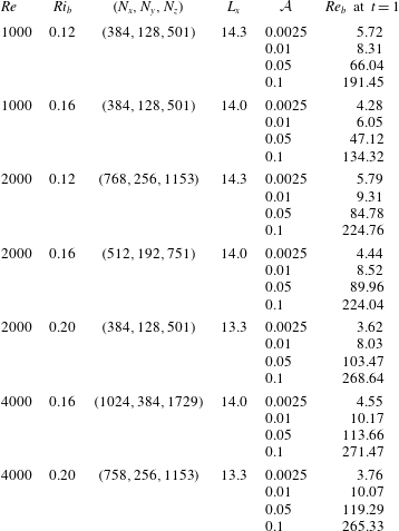
and corresponding grid sizes for each set of simulations are presented in table 1.
Flow parameters, grid sizes and initial turbulence strength of direct numerical simulations. All simulations shown have
 $Pr=1$
,
 $L_{y}=5.0$
and
 $L_{z}=25.0$
.

3 Results
Our goal is to explore mixing energetics in the three-dimensional space of initial parameter values
 $Re$
,
 $Ri_{b}$
and
 ${\mathcal{A}}$
. We begin by focusing on a single mean flow with
 $Re=2000$
and
 $Ri_{b}=0.16$
and comparing results with different
 ${\mathcal{A}}$
. We then repeat the analysis with different values of
 $Re$
and
 $Ri_{b}$
.
3.1 Effects of initial perturbation amplitude
In all simulations shown here there is a strong transient adjustment associated with the initial perturbation, with a decrease in kinetic energy, growth of buoyancy fluctuations and enhanced dissipation. This adjustment takes place over the first few non-dimensional time units, on scales comparable to the advective timescale (
 $t^{\ast }\sim h^{\ast }/U_{0}^{\ast }$
) and buoyancy timescale (
 $t^{\ast }\sim h^{\ast }/\sqrt{B_{0}}^{\ast }$
), both of which are
 $O(1)$
quantities when non-dimensionalized.
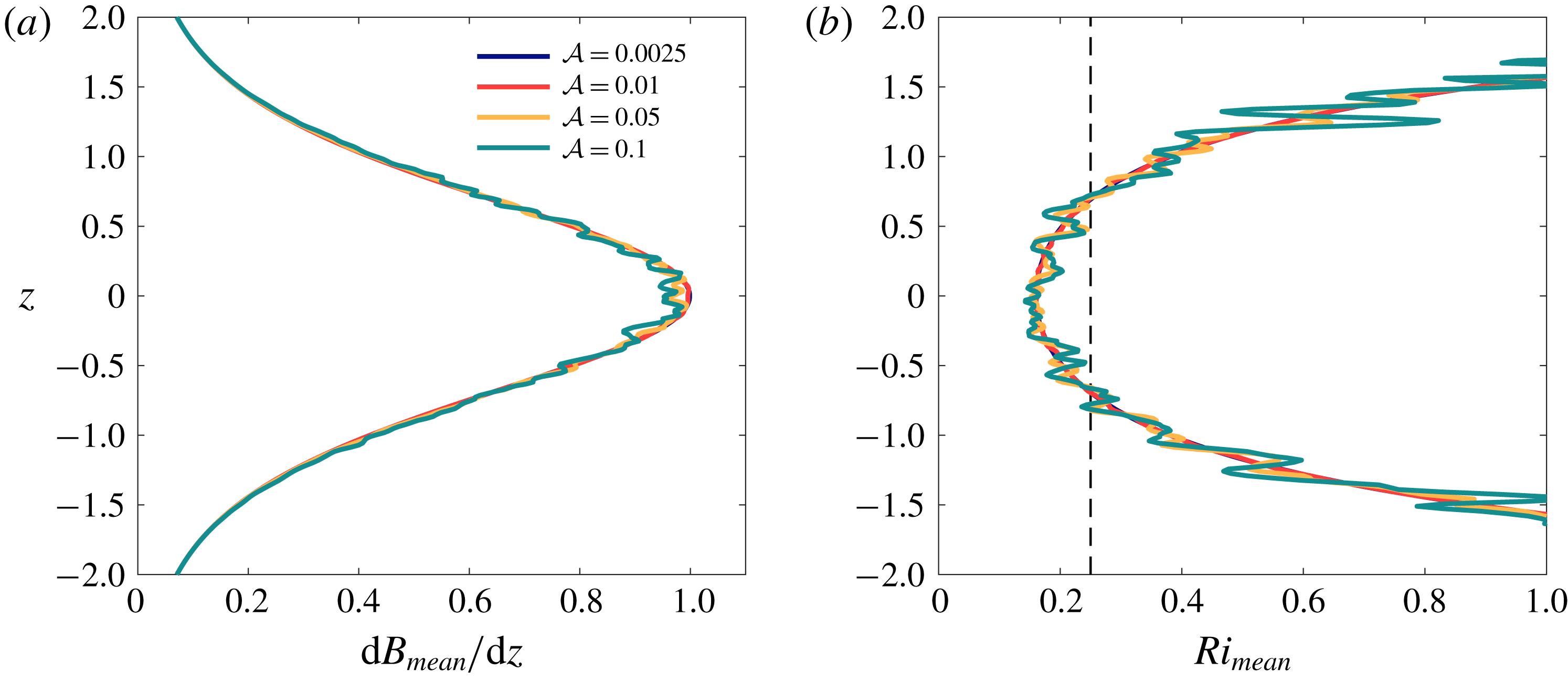
Profiles of the stratification and the gradient Richardson number of the mean flow (horizontally averaged) at
 $t=1$
(i.e. after the flow has started to adjust to the initial perturbation) are shown in figure 1. It is clear that the initial turbulence has led to a more complicated mean flow, particularly for the intermediate and strongly turbulent cases (
 ${\mathcal{A}}=0.05$
and
 ${\mathcal{A}}=0.1$
). However, it should be emphasized that in spite of the initial turbulence, the large-scale stratification still varies over the same length scale, and the mean Richardson number still exhibits a minimum on the order of
 $Ri_{b}$
. As such, the initial perturbation does not appear to significantly change the bulk stability of the flow.
Vertical profiles of (a) mean buoyancy gradient,
 $\text{d}B_{mean}/\text{d}z$
, and (b) gradient Richardson number of the mean flow,
 $Ri_{mean}$
at
 $t=1$
.
 $Ri=1/4$
is denoted by a thin dashed line in panel (b). Note that the line corresponding to
 ${\mathcal{A}}=0.0025$
lies almost directly beneath the line for
 ${\mathcal{A}}=0.01$
.

In addition to the characteristic amplitude of the velocity perturbation, we can further quantify the initial turbulence in terms of a buoyancy Reynolds number,
 $Re_{b}=\unicode[STIX]{x1D700}^{\ast }/\unicode[STIX]{x1D708}^{\ast }N^{\ast 2}$
, which describes the turbulence intensity. Characteristic values of
 $Re_{b}$
at
 $t=1$
corresponding to each individual simulation are listed in table 1. Values vary from
 $Re_{b}\lesssim 10$
for the laminar and weak initial turbulence cases (
 ${\mathcal{A}}=0.0025,0.01$
), at which viscous effects are expected to be important (Shih et al.
Reference Shih, Koseff, Ivey and Ferziger2005) to
 $Re_{b}\sim O(10^{2})$
for the strong initial turbulence cases, corresponding to highly energetic turbulence. For context, oceanic observations suggest a broad range of
 $Re_{b}\sim O(10)-O(10^{4})$
, with
 $Re_{b}\gtrsim 10^{2}$
during vigorous mixing (Smyth, Moum & Caldwell Reference Smyth, Moum and Caldwell2001).
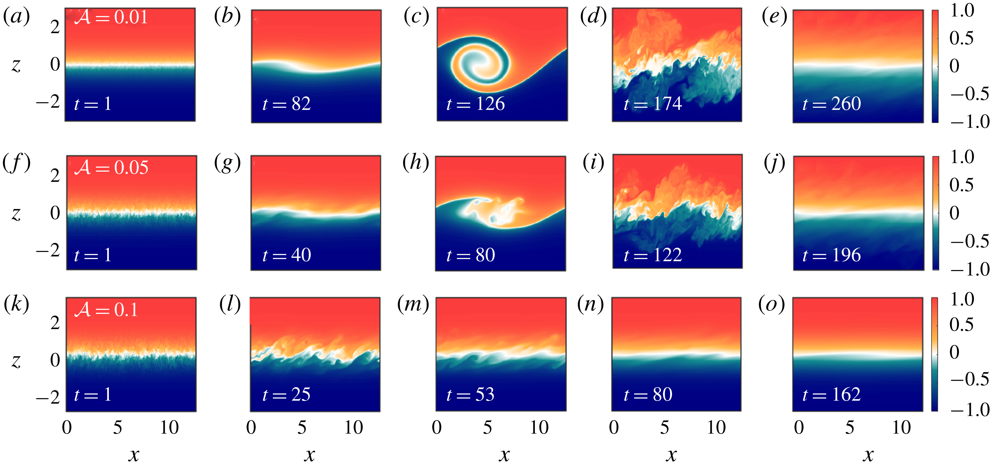
We now present a qualitative overview of the impact of perturbation amplitude on the evolution of the shear instability. Figure 2 shows vertical slices of buoyancy through
 $y=0$
at different times for cases with weak, intermediate and strong initial turbulence; the laminar case follows a very similar evolution to the case with weak initial turbulence and is therefore not shown here. For laminar and weakly turbulent initial conditions, the flow follows the usual lifecycle of a classical Kelvin–Helmholtz instability (Peltier & Caulfield Reference Peltier and Caulfield2003; Smyth & Moum Reference Smyth and Moum2012): two-dimensional perturbations grow and form finite-amplitude billows (figure 2
b,c), which are susceptible to three-dimensional secondary instabilities leading to a transition to turbulence (figure 2
d). As the flow considered here is unforced, it eventually relaminarizes after a period of turbulent mixing (figure 2
e).
As the initial perturbation amplitude is increased, the details of the flow evolution are modified. For the case of intermediate-amplitude initial turbulence (
 ${\mathcal{A}}=0.05$
, figure 2
f–j), a growing perturbation still leads to billow formation, transition to turbulence, and subsequent relaminarization. However, the growing perturbation is no longer two-dimensional, and the billow becomes turbulent much earlier in its development, without rolling up to the extent seen in the laminar and weakly turbulent cases (compare figure 2
c,h). As the strength of the initial perturbation is further increased, the characteristic billows associated with Kelvin–Helmholtz instability are no longer observed (figure 2
k–o). Instead, the initial turbulence fills the shear layer and subsequently decays.
Vertical slices of buoyancy through
 $y=0$
at various times for (a–e) weakly turbulent initial conditions (
 ${\mathcal{A}}=0.01$
), (f–j) intermediate initial conditions (
 ${\mathcal{A}}=0.05$
), and (k–o) strongly turbulent initial conditions (
 ${\mathcal{A}}=0.1$
). Non-dimensional times corresponding to each snapshot are shown in the bottom left corner of each panel.

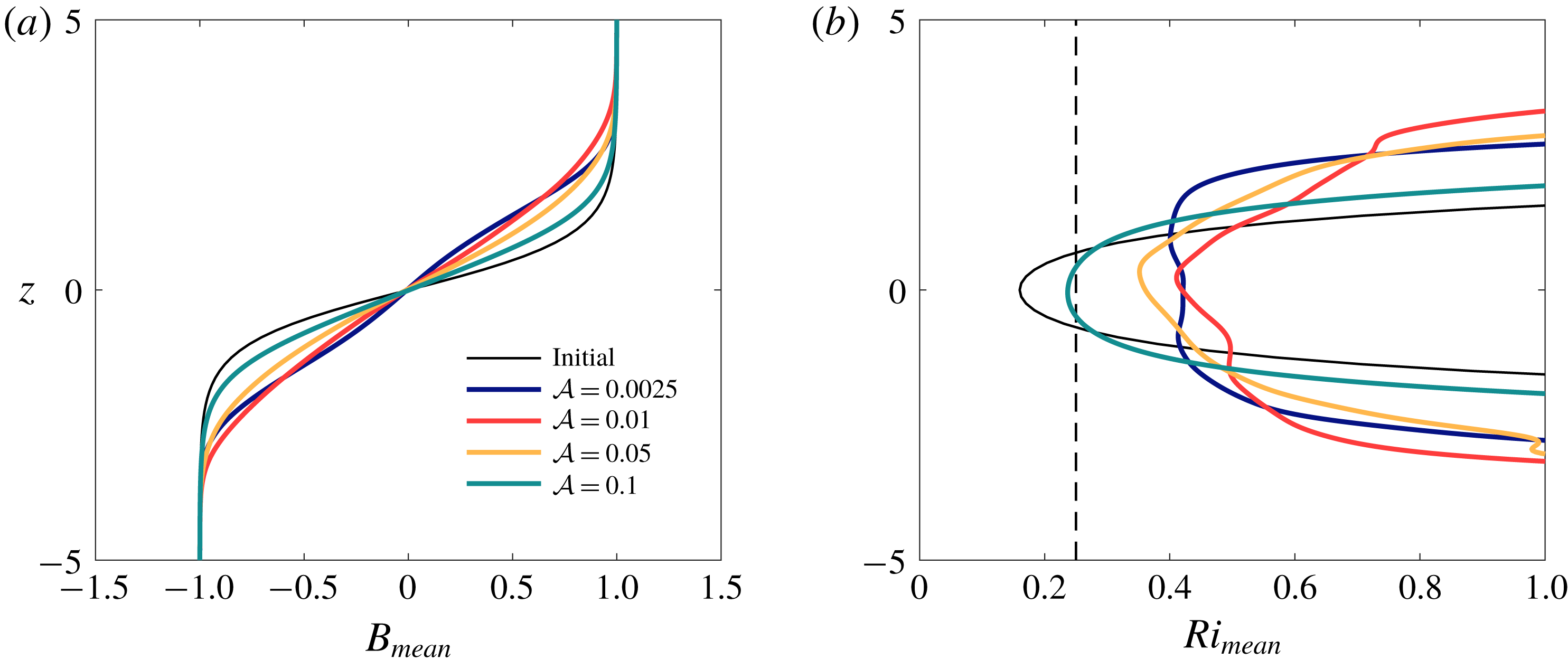
Figure 3(a) compares the initial buoyancy given in (2.2) with the horizontally-averaged buoyancy
 $B_{mean}$
after the flow has relaminarized. The vertical extent of the relaminarized layer depends strongly on whether finite-amplitude billows (figure 2
c,h) form and move denser fluid upwards (and vice versa). As a result, the final state of the flow with strongly turbulent initial conditions (without billow formation) has a much smaller vertical extent than any of the other cases shown. A similar trend is observed for the mean streamwise velocity (not shown here).
In addition to
 $B_{mean}$
, the gradient Richardson number of the final mean flow,
 $Ri_{mean}$
, is shown in figure 3(b). The minimum Richardson number at the end of the mixing event is well above the critical Miles-Howard value of
 $1/4$
for the laminar, weak and intermediate initial turbulence cases, consistent with experimental results suggesting that the Richardson number after a Kelvin–Helmholtz mixing event should lie in the range
 $0.32\pm 0.06$
(Thorpe Reference Thorpe1973). In contrast, strong initial turbulence results in much lower Richardson numbers after relaminarization. The final state is only marginally stable at the centre of the shear layer (green curve).
Initial (thin black lines) and final (thick coloured lines) vertical profiles of (a) mean buoyancy,
 $B_{mean}$
, and (b) gradient Richardson number of the mean flow,
 $Ri_{mean}$
.
 $Ri=1/4$
is denoted by a thin dashed line in panel (b).

The effect of varying the initial perturbation amplitude can be studied more quantitatively by considering the evolution of the total kinetic and potential energy of the flow. An equation governing the evolution of the kinetic energy,
 ${\mathcal{K}}\equiv \overline{u_{j}u_{j}/2}$
(where the overline denotes a volume average) is formed by taking the inner product of (2.3) with
 $\boldsymbol{u}$
and then averaging over the flow domain, i.e.
 $$\begin{eqnarray}\frac{\text{d}{\mathcal{K}}}{\text{d}t}={\mathcal{B}}-\unicode[STIX]{x1D700},\end{eqnarray}$$
where
 ${\mathcal{B}}\equiv Ri_{b}\overline{bw}$
is the vertical buoyancy flux and
 $\unicode[STIX]{x1D700}\equiv \overline{\unicode[STIX]{x2202}_{j}u_{i}\unicode[STIX]{x2202}_{j}u_{i}}/Re$
is the (positive-definite) kinetic energy dissipation. Similarly, an equation governing the total potential energy
 ${\mathcal{P}}=-Ri_{b}\overline{bz}$
is constructed by multiplying (2.4) by
 $Ri_{b}z$
and volume-averaging, i.e.
 $$\begin{eqnarray}\frac{\text{d}{\mathcal{P}}}{\text{d}t}=-{\mathcal{B}}+{\mathcal{D}}_{p},\end{eqnarray}$$
where
 ${\mathcal{D}}_{p}\equiv Ri_{b}(b_{top}-b_{bottom})/(RePrL_{z})$
denotes the change in potential energy due to diffusion of the mean laminar flow (i.e. the diffusive change in potential energy that would occur even in the absence of any fluid motion). In contrast, the buoyancy flux
 ${\mathcal{B}}$
describes the exchange of energy between kinetic and potential forms due to fluid motion, including both reversible stirring and irreversible mixing (Winters et al.
Reference Winters, Lombard, Riley and D’Asaro1995; Peltier & Caulfield Reference Peltier and Caulfield2003; Davies Wykes, Hughes & Dalziel Reference Davies Wykes, Hughes and Dalziel2015).
To isolate the irreversible mixing from the total buoyancy flux, we decompose the total potential energy into available and background components,
 ${\mathcal{P}}={\mathcal{P}}_{a}+{\mathcal{P}}_{b}$
. The background potential energy refers to the minimum potential energy state of the system which would be achieved by adiabatically rearranging the buoyancy field into a gravitationally stable configuration,
 $$\begin{eqnarray}{\mathcal{P}}_{b}=-Ri_{b}\overline{b^{\star }z}.\end{eqnarray}$$
The sorted profile
 $b^{\star }(z)$
may be calculated from the full three-dimensional buoyancy field either by sorting or by computing its probability density function, as we do here (Winters et al.
Reference Winters, Lombard, Riley and D’Asaro1995; Tseng & Ferziger Reference Tseng and Ferziger2001; Davies Wykes et al.
Reference Davies Wykes, Hughes and Dalziel2015). The available potential energy
 ${\mathcal{P}}_{a}$
is then the energy that may be used to mix the flow and arises due to horizontal buoyancy gradients or from statically-unstable regions of the flow (Lorenz Reference Lorenz1955). The governing equation for potential energy (3.2) can then be split into equations governing the evolution of these two components,
 $$\begin{eqnarray}\frac{\text{d}{\mathcal{P}}_{a}}{\text{d}t}=-{\mathcal{B}}-{\mathcal{M}},\quad \frac{\text{d}{\mathcal{P}}_{b}}{\text{d}t}={\mathcal{M}}+{\mathcal{D}}_{p}.\end{eqnarray}$$
It should be noted that Winters et al. (Reference Winters, Lombard, Riley and D’Asaro1995) refers to the sum of the terms
 ${\mathcal{M}}+{\mathcal{D}}_{p}$
as
 $\unicode[STIX]{x1D6F7}_{d}$
, describing the total change in background potential energy. However, here we are interested primarily in the irreversible mixing due to the evolution of the shear instability and its transition to turbulence. As such, we follow the convention of Peltier & Caulfield (Reference Peltier and Caulfield2003) and distinguish between changes in
 ${\mathcal{P}}_{b}$
due to fluid motion (described by
 ${\mathcal{M}}$
) and changes due to laminar diffusion of the mean flow (described by
 ${\mathcal{D}}_{p}$
).
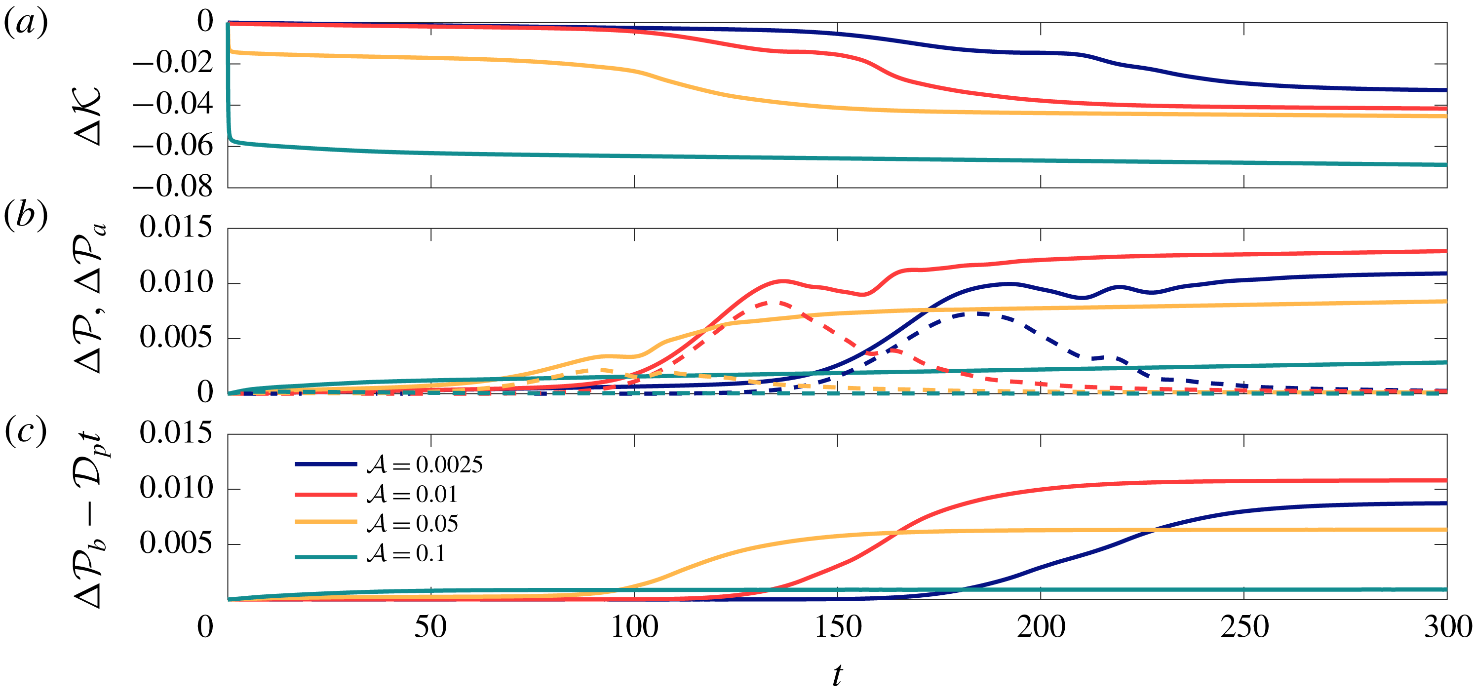
The evolution of the kinetic and potential energies are shown in figure 4. In the laminar and weakly turbulent cases (
 ${\mathcal{A}}=0.0025$
and
 $0.01$
; blue and red curves) there is little change in kinetic or potential energy until
 $t\sim 100$
when the linearly-growing perturbation reaches finite amplitude. The change in
 ${\mathcal{P}}$
is initially associated with the growth of available potential energy arising from the formation of the billow structure. Then, as the secondary instabilities grow and trigger turbulence, the background potential energy begins to increase irreversibly while the available potential energy decays. Finally, as the flow relaminarizes, the energy changes approach near-constant values.
For the case with strongest initial turbulence (
 ${\mathcal{A}}=0.1$
; green curves), the energy evolves in a very different manner, as might be expected based on the buoyancy evolution (figure 2
k–o). The kinetic and potential energies change quickly as the initial turbulence decays and mixes the mean flow (also seen to some extent for the case with intermediate initial turbulence). Changes in available potential energy are small, and changes in total potential energy largely correspond to changes in
 ${\mathcal{P}}_{b}$
from irreversible mixing. After the initial vigorous mixing, the small remaining changes in energy are largely due to the effects of viscosity and diffusion on the relaminarized mean flow, with a plateau in
 ${\mathcal{P}}_{b}-{\mathcal{D}}_{p}t$
(figure 4
c), and no further increases associated with the growth of the Kelvin–Helmholtz instability.
The case with intermediate-amplitude initial turbulence (
 ${\mathcal{A}}=0.05$
; yellow curves) shares features of both the weak and strong initial turbulence cases. There is an initial change in kinetic and potential energy owing to the turbulent initial conditions. Then, as the billow begins to form (figure 2
h), available potential energy rises, as for the classical Kelvin–Helmholtz instability. However, the flow becomes turbulent before the billow forms completely, and correspondingly the growth of
 ${\mathcal{P}}_{a}$
is arrested as
 ${\mathcal{P}}_{b}$
begins to rise due to turbulent mixing. Finally, as in the other three cases, the energies plateau as the turbulence decays and the flow relaminarizes. Overall potential energy changes depend non-monotonically on the perturbation amplitude: larger changes in total and background potential energy are observed for
 ${\mathcal{A}}=0.01$
when compared with
 ${\mathcal{A}}=0.0025$
and
 ${\mathcal{A}}=0.05$
.
Time evolution of changes in (a) kinetic energy
 ${\mathcal{K}}$
, (b) total potential energy
 ${\mathcal{P}}$
(solid) and available potential energy
 ${\mathcal{P}}_{a}$
(dashed), and (c) background potential energy associated with fluid motion,
 ${\mathcal{P}}_{b}-{\mathcal{D}}_{p}t$
.

Using the above description of the flow energetics, the mixing efficiency can be defined instantaneously as
 $$\begin{eqnarray}\unicode[STIX]{x1D702}_{i}=\frac{{\mathcal{M}}}{{\mathcal{M}}+\unicode[STIX]{x1D700}}.\end{eqnarray}$$
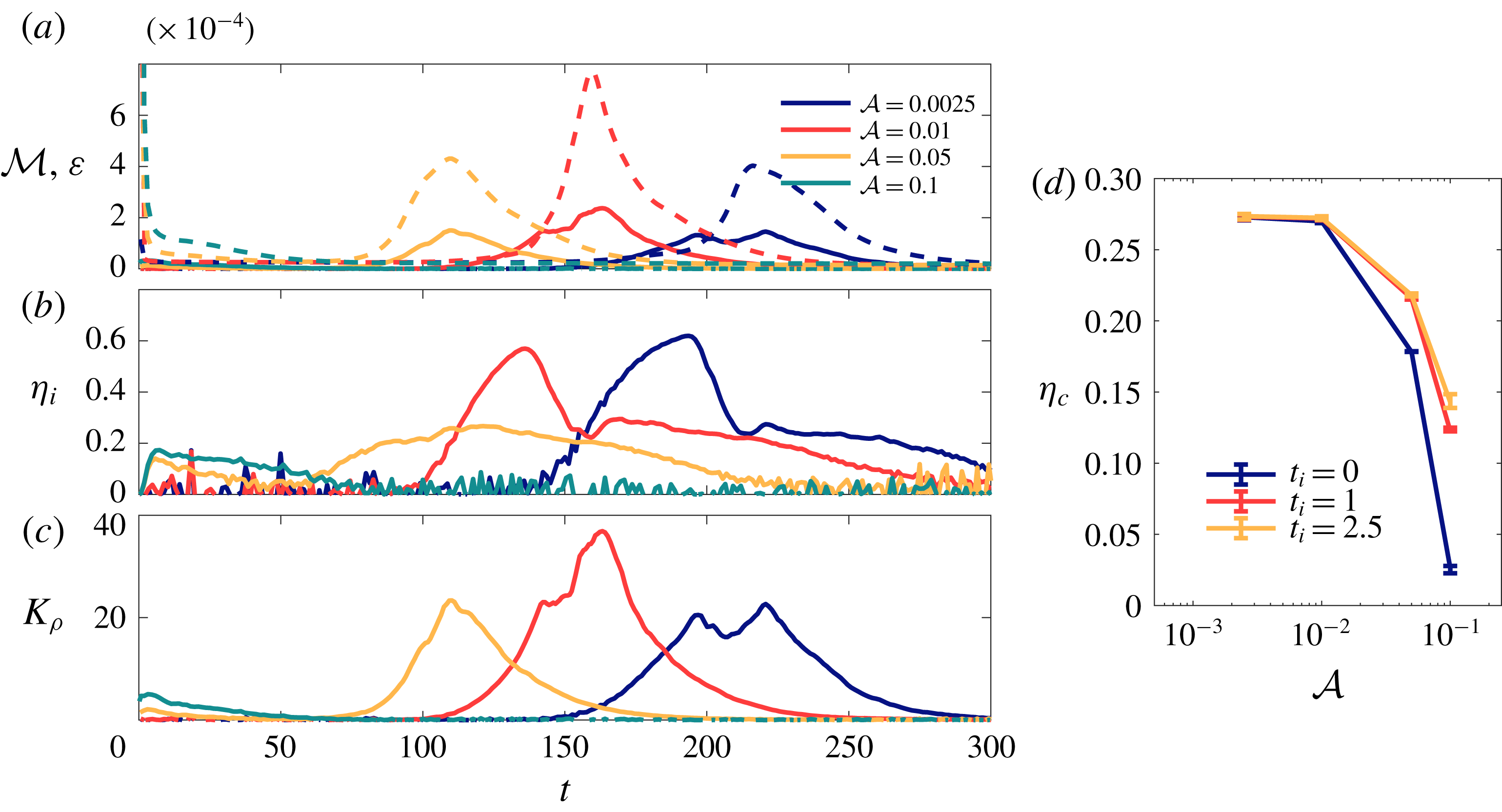
In the laminar and weak turbulence cases, the evolution of
 ${\mathcal{M}}$
,
 $\unicode[STIX]{x1D700}$
and
 $\unicode[STIX]{x1D702}_{i}$
(blue and red curves, figure 5
a,b) is similar to that found in previous studies of mixing by Kelvin–Helmholtz instability (Smyth et al.
Reference Smyth, Moum and Caldwell2001; Peltier & Caulfield Reference Peltier and Caulfield2003; Mashayek et al.
Reference Mashayek, Caulfield and Peltier2013). There is an initial phase during which the irreversible mixing rate is larger than the dissipation, with very high mixing efficiency,
 $\unicode[STIX]{x1D702}_{i}\sim 0.6$
. This occurs shortly after the peak in available potential energy (figure 4
b), and is associated with the rollup of the shear instability into the classical billow structure. Then, as the flow becomes turbulent, the mixing efficiency drops to a value
 $\unicode[STIX]{x1D702}_{i}\sim 0.3$
as
 $\unicode[STIX]{x1D700}$
peaks. As the flow relaminarizes,
 ${\mathcal{M}}\rightarrow 0$
while
 $\unicode[STIX]{x1D700}$
remains non-zero owing to the continued viscous dissipation of the mean flow, and so
 $\unicode[STIX]{x1D702}_{i}$
decreases further.
(a) Time variation of mixing rate,
 ${\mathcal{M}}$
(solid), and dissipation,
 $\unicode[STIX]{x1D700}$
(dashed). (b) Time variation of instantaneous mixing efficiency,
 $\unicode[STIX]{x1D702}_{i}$
. (c) Time variation of turbulent diffusivity,
 $K_{\unicode[STIX]{x1D70C}}$
. (d) Cumulative mixing efficiencies
 $\unicode[STIX]{x1D702}_{c}$
calculated over an entire mixing event for three definitions of the initial time
 $t=t_{i}$
. The error bars correspond to mixing efficiencies calculated with final times
 $t_{f}={\mathcal{D}}_{p}/2$
and
 $t_{f}=2{\mathcal{D}}_{p}$
.

In cases with increased initial perturbation amplitude, the mixing efficiency evolves differently. As figure 2 shows, the billow structure breaks down into turbulence much earlier in the case of intermediate initial turbulence, without rolling up to the same extent as in the classical Kelvin–Helmholtz case. Correspondingly, the peak in
 $\unicode[STIX]{x1D702}_{i}$
associated with laminar rollup of the billow is absent, and the instantaneous irreversible mixing rate
 ${\mathcal{M}}$
is always less than the dissipation
 $\unicode[STIX]{x1D700}$
(yellow curves, figure 5
a,b). The maximum instantaneous mixing efficiency in this case is only approximately
 $0.35$
, as in the later turbulent mixing stage of the lower initial amplitude cases. As the initial perturbation amplitude is further increased and the billow structure no longer arises (figure 2
k–o), the mixing efficiency only achieves values of approximately
 $0.2$
during the initial turbulent mixing phase before decaying at later times.
As with the overall changes in potential energy shown in figure 4(b,c), the peak value of the irreversible mixing rate and the dissipation depend non-monotonically on the initial perturbation amplitude
 ${\mathcal{A}}$
, with maximum values occurring for
 ${\mathcal{A}}=0.01$
. Indeed, the maximum values of both
 ${\mathcal{M}}$
and
 $\unicode[STIX]{x1D700}$
are very similar for the laminar (
 ${\mathcal{A}}=0.0025$
) and intermediate initial turbulence (
 ${\mathcal{A}}=0.05$
) cases, despite the marked differences in both instantaneous and cumulative mixing efficiencies between these two cases. This further emphasizes the role of the highly-efficient pre-turbulent phase associated with billow rollup in determining the overall efficiency of a given mixing event.
As mentioned above, the viscous dissipation can be related to a turbulent density flux via a turbulent diffusivity,
 $K_{\unicode[STIX]{x1D70C}}$
, expressed in non-dimensional form as (Salehipour & Peltier Reference Salehipour and Peltier2015)
 $$\begin{eqnarray}K_{\unicode[STIX]{x1D70C}}=\unicode[STIX]{x1D6E4}PrRe_{b}=\frac{\unicode[STIX]{x1D702}}{1-\unicode[STIX]{x1D702}}PrRe_{b}.\end{eqnarray}$$
All cases show non-zero values of
 $K_{\unicode[STIX]{x1D70C}}$
at similar times to the changes in
 ${\mathcal{P}}_{b}$
(figure 4
c). For strongly turbulent initial conditions (
 ${\mathcal{A}}=0.1$
, green line in figure 5
c), there is a small increase in
 $K_{\unicode[STIX]{x1D70C}}$
at early times and then subsequent decay. For the other three cases, much larger peak values of
 $K_{\unicode[STIX]{x1D70C}}$
are observed. In all three cases there is a peak in
 $K_{\unicode[STIX]{x1D70C}}$
associated with peak values of
 $\unicode[STIX]{x1D700}$
(and peak values of
 $Re_{b}$
, not shown), with the highest values associated with
 ${\mathcal{A}}=0.01$
. However, there is an additional peak for the two cases in which billow formation was not impeded (
 ${\mathcal{A}}=0.0025$
and
 $0.01$
). This peak is associated with the onset of turbulence after the rolling up of the billows and the associated peak in mixing efficiency. While the viscous dissipation is still relatively low at this point in the flow evolution, the highly efficient motions lead to a correspondingly high turbulent buoyancy flux. As a result,
 $K_{\unicode[STIX]{x1D70C}}$
remains elevated for a much longer period of time in these two cases relative to the case with intermediate initial turbulence (
 ${\mathcal{A}}=0.05$
), leading to larger changes overall in the background potential energy.
It is also of interest to describe an individual mixing event in terms of an overall mixing efficiency. A cumulative analogue to (3.5) is defined by integrating
 ${\mathcal{M}}$
and
 $\unicode[STIX]{x1D700}$
over the duration of a mixing event (from some initial time
 $t_{i}$
to some final time
 $t_{f}$
) as
 $$\begin{eqnarray}\unicode[STIX]{x1D702}_{c}=\frac{\displaystyle \int _{t_{i}}^{t_{f}}{\mathcal{M}}\,\text{d}t}{\displaystyle \int _{t_{i}}^{t_{f}}{\mathcal{M}}\,\text{d}t+\int _{t_{i}}^{t_{f}}\unicode[STIX]{x1D700}\,\text{d}t}.\end{eqnarray}$$
As previously discussed, and as figures 4 and 5(a) show, there is a strong initial transient adjustment for the cases with intermediate and strong initial turbulence. We find that the computed values of
 $\unicode[STIX]{x1D702}_{c}$
are sensitive to initial integration times
 $t_{i}$
within this adjustment period until approximately
 $t_{i}\sim 1$
; the computed values of
 $\unicode[STIX]{x1D702}_{c}$
do not change significantly for
 $1\lesssim t_{i}\lesssim 10$
. We define
 $t_{f}$
as the time when
 ${\mathcal{M}}={\mathcal{D}}_{p}$
after the mixing event, i.e. the time at which changes in
 ${\mathcal{P}}_{b}$
due to turbulent mixing become comparable to changes due to laminar diffusion in the absence of fluid motion. Note, however, that the computed mixing efficiencies in figure 5(d) are not strongly sensitive to the choice of
 $t_{f}$
, as long as
 $t_{f}$
is after the shear layer begins to relaminarize.
The cases with laminar and weakly turbulent initial conditions (i.e. the cases that follow a typical Kelvin–Helmholtz lifecycle) yield similar cumulative mixing efficiencies,
 $\unicode[STIX]{x1D702}_{c}\approx 0.27$
, consistent with previous results for simulations of the Kelvin–Helmholtz instability (Peltier & Caulfield Reference Peltier and Caulfield2003; Mashayek et al.
Reference Mashayek, Caulfield and Peltier2013). As the initial perturbation amplitude is increased and the large peak in
 $\unicode[STIX]{x1D702}_{i}$
associated with laminar rollup is lost,
 $\unicode[STIX]{x1D702}_{c}$
decreases to values of approximately
 $0.18$
for
 $t_{i}=0$
in the intermediate initial turbulence case and
 $0.025$
in the strong initial turbulence case. This decrease in
 $\unicode[STIX]{x1D702}_{c}$
is consistent with the evolution of
 ${\mathcal{M}}$
,
 $\unicode[STIX]{x1D700}$
and
 $\unicode[STIX]{x1D702}_{i}$
for these amplitudes: irreversible mixing is essentially restricted to times when the flow is turbulent, without the highly efficient pre-turbulent phase associated with billow structure and its large available potential energy. If the initial transient adjustment is excluded (
 $t_{i}\geqslant 1$
),
 $\unicode[STIX]{x1D702}_{c}$
increases to values of approximately
 $0.22$
and
 $0.13$
for
 ${\mathcal{A}}=0.05$
and
 ${\mathcal{A}}=0.1$
, respectively. This increase in
 $\unicode[STIX]{x1D702}_{c}$
is due to the fact that, at very early times, the buoyancy field has not yet adjusted to the initial perturbation, and so the flow is dissipating kinetic energy without mixing buoyancy.
3.2
 $Re$
and
$Ri_{b}$
effects


Thus far, we have focused on a single choice of the mean flow parameters
 $Re$
and
 $Ri_{b}$
, showing that turbulent initial conditions can impact the evolution of a stratified shear layer. To examine the effect of the mean flow parameters, we now consider simulations at a variety of initial
 $Re$
and
 $Ri_{b}$
for the same four values of
 ${\mathcal{A}}$
as considered in the previous section. While the initial perturbation varies slightly depending on the domain size and grid resolution (and, therefore, the corresponding values of
 $k_{h}$
in (2.8)), the kinetic energy of the initial perturbation and the turbulence intensity at early times are similar for the same value of
 ${\mathcal{A}}$
across the range of simulations presented in table 1.
Billow growth due to shear instability is associated with an increase in the available potential energy,
 ${\mathcal{P}}_{a}$
. As such, we look for local maxima in the growth rate of available potential energy,
 $\text{d}{\mathcal{P}}_{a}/\text{d}t$
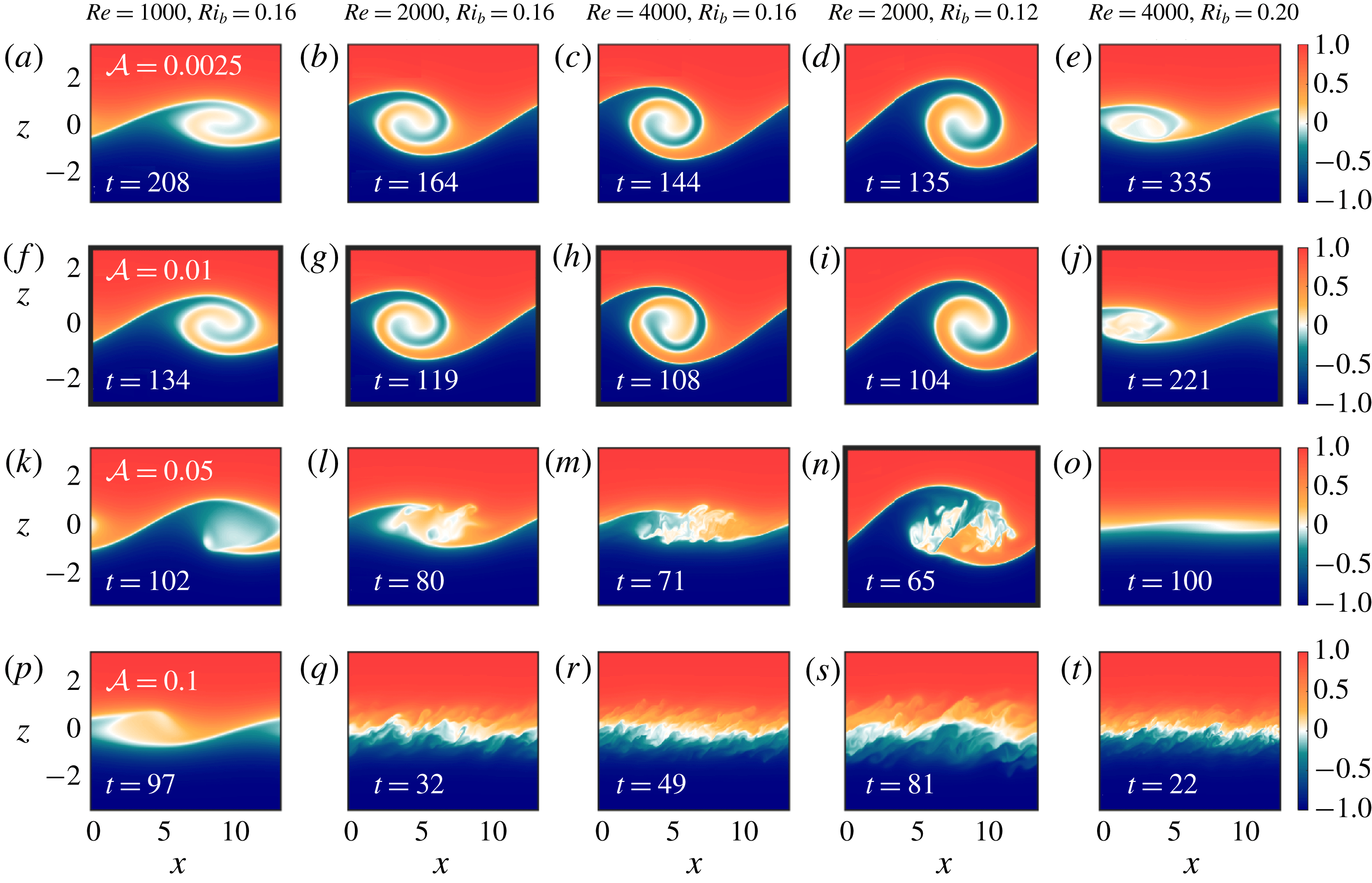
, as a means of identifying billows in our suite of simulations. In figure 6 we show the billow structure corresponding to a range of different values of
 $Re$
and
 $Ri_{b}$
and all four values of
 ${\mathcal{A}}$
, identified using this metric. Note that the specific times corresponding to each snapshot in figure 6 differ depending on both the flow parameters and the initial perturbations. Finite-amplitude billows typically form at later non-dimensional times for higher values of
 $Ri_{b}$
(owing to the slower growth rate of the underlying shear instability) and earlier for higher
 ${\mathcal{A}}$
(owing to the larger amount of energy initially present in the unstable mode). However, despite the different times highlighted in figure 6, for the cases with clear billow structures the instability follows a similar evolution to that shown in figure 2: the billow becomes unstable to secondary instabilities, the shear becomes fully turbulent, and after some time the turbulence decays and the flow relaminarizes.
Vertical slices of buoyancy through
 $y=0$
at various times corresponding to local maxima in
 $\text{d}{\mathcal{P}}_{a}/\text{d}t$
. (a–e) Laminar initial conditions,
 ${\mathcal{A}}=0.0025$
. (f–j) Weakly turbulent initial conditions,
 ${\mathcal{A}}=0.01$
. (k–o) Intermediate turbulence initial conditions,
 ${\mathcal{A}}=0.05$
. (p–t) Strongly turbulent initial conditions,
 ${\mathcal{A}}=0.1$
. Each column corresponds to a different set of simulations with the specified values of
 $Re$
and
 $Ri_{b}$
. Non-dimensional times corresponding to each snapshot are shown in the bottom left corner of each panel. Panels with thick black borders correspond to the value of
 ${\mathcal{A}}$
which gives the maximum change in
 ${\mathcal{P}}_{b}$
for a given
 $(Re,Ri_{b})$
.

Several trends become apparent upon consideration of figure 6. As the initial turbulence amplitude is increased, the development of the shear instability is accordingly modified: the billow structure becomes susceptible to secondary instabilities before fully rolling up, and is prevented from forming for strongly turbulent initial conditions (as shown in the bottom two rows of figure 6). This effect is consistent across the range of
 $Re$
and
 $Ri_{b}$
investigated here.
However, figure 6 also reveals additional effects related to the initial mean flow parameters. The initial Reynolds number of the shear layer appears to affect the sensitivity of the billow structure to modification by pre-existing turbulence. For example, with lower
 $Re$
and weak initial turbulence (figure 6
f,g,i), the resulting billow appears similar to the corresponding structure with laminar initial conditions (figure 6
a,b,d). However, as
 $Re$
is increased, the billow structure is modified; for example, in comparing figures 6(c) and 6(h), it is clear that the weak initial turbulence has led to asymmetry in the fully developed billow before transition to turbulence. Similarly,
 $Re$
effects are apparent for the partially developed billows in the case of intermediate initial turbulence. As figure 6(k,l,m) show, when the Reynolds number is increased for the same initial
 $Ri_{b}$
, the height of the overturn before breaking down into turbulence is decreased (figure 6
k,l,m).
Figure 6 also suggests a strong dependence on the initial bulk Richardson number,
 $Ri_{b}$
. The underlying shear instability is less sensitive to the initial turbulence at lower
 $Ri_{b}$
, with the billow able to grow to its full vertical height even in the presence of intermediate initial turbulence (figure 6
n). At the other extreme, for higher
 $Ri_{b}$
, intermediate initial turbulence is sufficiently strong to almost prevent billow formation altogether (figure 6
o).
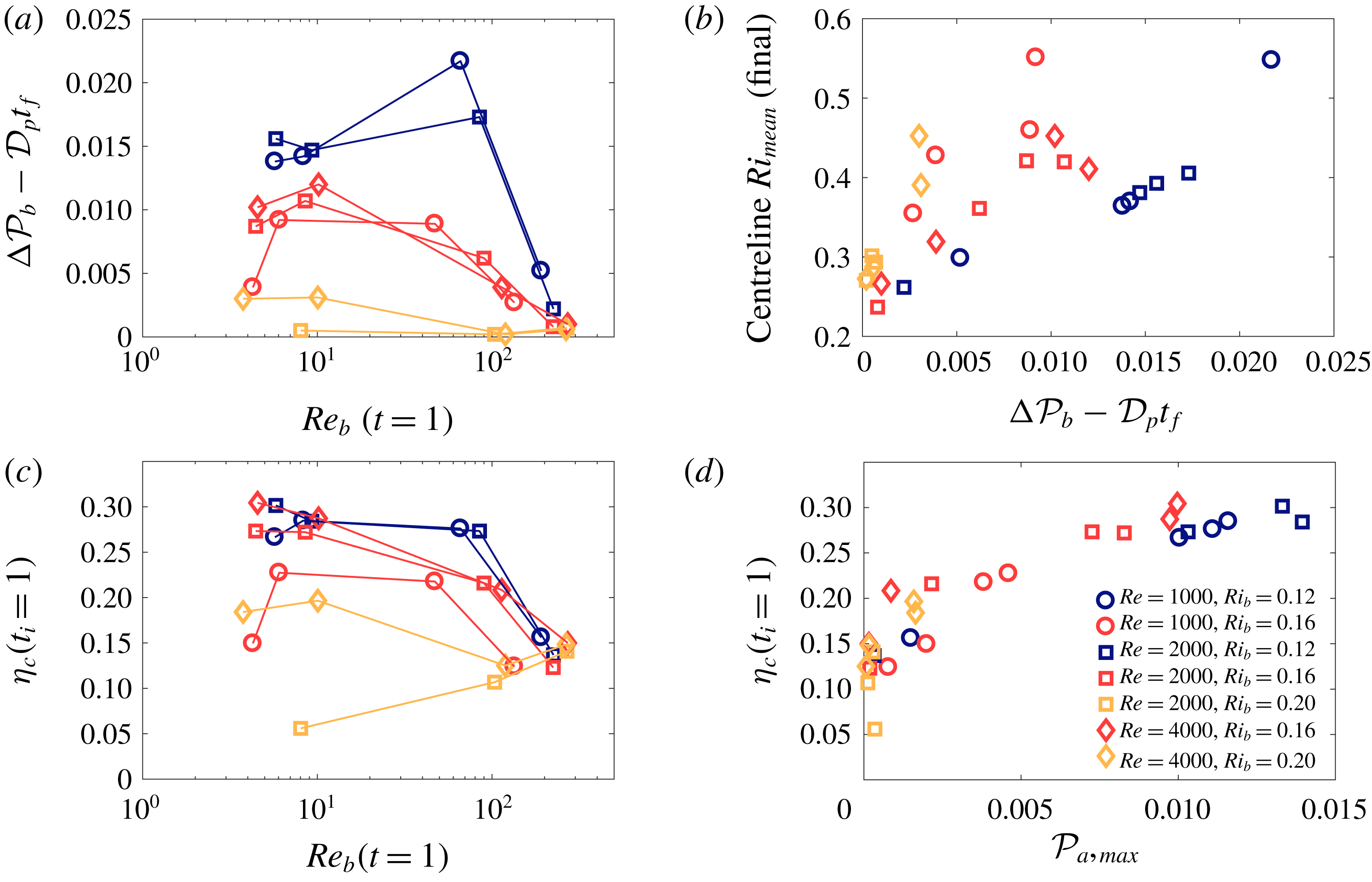
Figure 7(a) shows the overall change in potential energy associated with turbulent irreversible mixing (i.e.
 $\unicode[STIX]{x0394}{\mathcal{P}}_{b}-{\mathcal{D}}_{p}t$
) as a function of the buoyancy Reynolds number at
 $t=1$
. As observed in figure 4(b), there is a non-monotonic variation of total change in
 ${\mathcal{P}}_{b}$
with
 $Re_{b}$
. The specific amplitude at which the change in background potential energy peaks depends on
 $Ri_{b}$
: while the cases with
 $Ri_{b}=0.16$
(all
 $Re$
) and the cases with
 $Ri_{b}=0.20$
and
 $Re=4000$
exhibit maximum mixing for weak initial turbulence (
 ${\mathcal{A}}=0.01$
), the cases with
 $Ri_{b}=0.12$
instead show a clear peak for intermediate initial conditions (
 ${\mathcal{A}}=0.05$
). This can be understood by considering again the billow structures in figure 6 – in particular, those cases indicated by thick black borders which correspond to the large changes in
 ${\mathcal{P}}_{b}$
. The cases with the most mixing correspond to cases in which there is some initial turbulence present, but not so much as to prevent the billow from growing to its maximum vertical extent. That is, the overturn associated with the underlying instability is able to reach its maximum amplitude, but then transitions to turbulence before completely rolling up. This is especially noticeable in figure 6(n). As initial turbulence strength is further increased and the billow structure is not able to form completely (e.g. figure 6
k,l,m), the total change in background potential energy correspondingly begins to decrease. Finally, very small changes in background potential energy are observed for strong initial turbulence across the range of
 $Re$
and
 $Ri_{b}$
considered here. The primary exception to this trend is the set of simulations with
 $Ri_{b}=0.20$
and
 $Re=2000$
(yellow squares), in which diffusion of the mean flow plays a significant role before the instability can reach finite amplitude for
 ${\mathcal{A}}=0.0025$
and
 ${\mathcal{A}}=0.01$
; for these cases, very little mixing occurs due to a lack of vigorous turbulence.
(a) Overall potential energy change due to irreversible mixing,
 ${\mathcal{P}}_{b}-D_{p}t$
, as a function of
 $Re_{b}$
at
 $t=1$
. (b) Final centreline
 $Ri_{mean}$
as a function of
 ${\mathcal{P}}_{b}-D_{p}t$
. (c) Cumulative mixing efficiency,
 $\unicode[STIX]{x1D702}_{c}$
, calculated with
 $t_{i}=1$
and
 $t_{f}$
corresponding to
 ${\mathcal{M}}={\mathcal{D}}_{p}$
as a function of
 $Re_{b}$
at
 $t=1$
for a range of different
 $Re$
and
 $Ri_{b}$
. (d) Cumulative mixing efficiency,
 $\unicode[STIX]{x1D702}_{c}$
, as a function of the maximum available potential energy during a simulation,
 ${\mathcal{P}}_{a,max}$
.

As figure 3(b) shows, the stability of the final mean flow (quantified by its Richardson number) also depends on the initial turbulence amplitude. In figure 7(b) we show the final value of
 $Ri_{mean}$
at the centre of the shear layer after the mixing event as a function of total change in
 ${\mathcal{P}}_{b}$
. Unsurprisingly, there is a clear relationship between the total amount of irreversible mixing that occurs and the stability of the final flow, with large values of
 $\unicode[STIX]{x0394}{\mathcal{P}}_{b}-{\mathcal{D}}_{p}t_{f}$
leading to large values of centreline
 $Ri_{mean}$
. This trend is observed across the range of simulations presented here, suggesting that the degree to which a billow is able to form determines the degree to which the mean flow is stabilized.
Our analysis of the cases with
 $Re=2000$
and
 $Ri_{b}=0.16$
in the previous subsection showed a strong dependence of the cumulative mixing efficiency on the initial perturbation amplitude, with values dropping from
 $\unicode[STIX]{x1D702}_{c}\approx 0.27$
to
 ${\sim}0.13$
as the initial turbulence amplitude is increased (figure 5
d). This trend is observed for the majority of the cases considered here: individual mixing events are typically more efficient for lower values of
 ${\mathcal{A}}$
(figure 7
c). There is, however, a clear dependence of the mixing efficiency on
 $Ri_{b}$
, with much higher cumulative mixing efficiencies (
 ${\sim}0.3$
) observed for cases with
 $Ri_{b}=0.12$
and lower efficiencies (
 ${\sim}0.2$
) for cases with
 $Ri_{b}=0.20$
. As with the total change in background potential energy, the main exceptions to this trend are cases in which turbulence is weak and, therefore, the diffusion of the background flow plays an important role, namely, the cases with
 $Re=2000$
and
 $Ri_{b}=0.20$
, as well as the simulation with
 $Re=1000$
,
 $Ri_{b}=0.16$
and
 ${\mathcal{A}}=0.002$
. The largest overall change in potential energy is not necessarily associated with more efficient mixing (compare figure 7
a,c).
In the previous subsection we showed that a key factor in the efficiency of each mixing event is the degree to which the billow structure, with its associated pre-turbulent peak in instantaneous mixing efficiency, is able to form. Given that the available potential energy
 ${\mathcal{P}}_{a}$
increases with the size of the billow structure (see figure 4
b), we can use the maximum value of
 ${\mathcal{P}}_{a}$
as a measure of billow development. Figure 7(d) shows the cumulative mixing efficiency for each of our simulations as a function of
 ${\mathcal{P}}_{a,max}$
. There is a clear trend in the efficiency of our simulated mixing events across all values of
 $Re$
,
 $Ri_{b}$
and
 ${\mathcal{A}}$
considered here. The cases with strong initial turbulence in which there is little billow growth (and, accordingly,
 ${\mathcal{P}}_{a,max}$
is small) have lower mixing efficiencies of the order of
 $\unicode[STIX]{x1D702}_{c}\sim 0.1{-}0.15$
. When larger overturns are able to form and
 ${\mathcal{P}}_{a,max}$
increases, the mixing efficiency also increases before eventually reaching a plateau at values of
 $\unicode[STIX]{x1D702}_{c}\sim 0.3$
, consistent with values from previous studies of the Kelvin–Helmholtz instability in laminar initial flows (Peltier & Caulfield Reference Peltier and Caulfield2003; Mashayek et al.
Reference Mashayek, Caulfield and Peltier2013; Mashayek & Peltier Reference Mashayek and Peltier2013). This trend even includes the previously identified outlier cases from figure 7(a,c) in which diffusion of the background flow played a key role and led to smaller maximum billow sizes (figure 6
a).
Altogether, figures 6 and 7 demonstrate that initial turbulence significantly affects the development of a stratified shear layer, both qualitatively and quantitatively, across a range of
 $Re$
and
 $Ri_{b}$
. These effects are consistent with the results presented in § 3.1, in which initial turbulence may impede the development of the classical Kelvin–Helmholtz billow and, thus, alter the details of the turbulent mixing. For similar initial turbulence amplitudes, these effects appear more pronounced for higher
 $Re$
and higher
 $Ri_{b}$
, suggesting a relationship between the rate of decay of the initial turbulence (which is slower for higher
 $Re$
) and the growth rate of the underlying instability (which increases for lower
 $Ri_{b}$
).
4 Discussion and conclusions
We have shown that the evolution of a dynamically-unstable shear layer may be significantly modified in the presence of pre-existing turbulence, such as may be left behind after a previous mixing event. For small perturbation amplitudes, the classical Kelvin–Helmholtz instability is observed, and the energy evolution and irreversible mixing evolve in a manner similar to that found in previous studies of laminar stratified shear layers. However, as the perturbation amplitude is increased, the development of the canonical billow structure is first suppressed (with transition to turbulence occurring before the billow fully wraps up) and then is eliminated altogether. The latter finding is consistent with the results of Brucker & Sarkar (Reference Brucker and Sarkar2007). The total change to the background potential energy (a measure of the total amount of mixing) depends non-monotonically on the initial perturbation amplitude, reaching a maximum when initial turbulence is present but insufficient to prevent the billow from reaching its maximum vertical extent. The instantaneous and cumulative mixing efficiencies depend strongly on whether a Kelvin–Helmholtz billow forms, and decrease as the initial turbulence amplitude is increased. The effects of initial turbulence on the shear layer development are observed for a range of Reynolds and initial bulk Richardson numbers. Modifications of the billow structure associated with the underlying Kelvin–Helmholtz instability are seen for lower initial perturbation amplitudes at higher
 $Re$
and higher
 $Ri_{b}$
.
Overturns associated with shear instability are frequently observed in the atmosphere and oceans. However, the characteristic rolled up structure typically found in numerical simulations of the Kelvin–Helmholtz instability (figure 2
c) is not often seen (e.g. van Haren et al.
Reference van Haren, Gostiaux, Morozov and Tarakanov2014; Holleman et al.
Reference Holleman, Geyer and Ralston2016). The associated mixing efficiencies are much lower than the values of
 ${\sim}1/3$
found in previous numerical studies, suggesting that the pre-turbulent rollup associated with the formation of the billow may be less important in true geophysical flows (Holleman et al.
Reference Holleman, Geyer and Ralston2016). In their recent review Gregg et al. (Reference Gregg, D’Asaro, Riley and Kunze2018) suggested several possibilities to explain this mismatch between observations and simulations, including differences in parameter values (including
 $Re_{b}$
and
 $Pr$
), non-Boussinesq effects and differences between the mechanisms driving mixing in highly-idealized simulations versus field measurements. Consistent with this final point, our results (especially our intermediate-amplitude case with its partial billow formation) suggest that pre-existing turbulence may play an important role. In particular, the question of how important the highly efficient pre-turbulent rollup is in shear instabilities may have implications for the parameterization of turbulent mixing events in oceanographic flows (Mashayek et al.
Reference Mashayek, Salehipour, Bouffard, Caulfield, Ferrari, Nikurashin, Peltier and Smyth2017a
).
Recent work by Mashayek, Caulfield & Peltier (Reference Mashayek, Caulfield and Peltier2017b
) examining the length scales characterizing turbulent mixing arising from a Kelvin–Helmholtz instability suggests that stratified turbulence is most efficient when distinct overturns exist. Their results suggest that this state of maximum efficiency corresponds to times when the Thorpe length (quantifying the size of the overturns) and the Ozmidov length (quantifying the size at which background stratification is important) are comparable. They argue that these overturns, associated with secondary instabilities, are able to feed off the stored available potential energy in the Kelvin–Helmholtz billow structure and, thereby, efficiently drive the turbulent cascade of energy to small scales. Our results, summarized in figure 7(d), are broadly consistent with this conjecture, insofar as we observe less efficient mixing as
 ${\mathcal{A}}$
is increased and the primary Kelvin–Helmholtz billow either becomes turbulent before rolling up and storing
 ${\mathcal{P}}_{a}$
(
 ${\mathcal{A}}=0.05$
) or fails to form at all (
 ${\mathcal{A}}=0.1$
). Future work will consider how pre-existing turbulence modifies the evolution of these turbulent length scales.
While we have considered a range of
 $Re$
and
 $Ri_{b}$
here, we have kept the Prandtl number fixed at
 $Pr=1$
for all of the simulations presented above. Previous studies have shown that the transition to turbulence and mixing observed for the Kelvin–Helmholtz instability depends on the value of
 $Pr$
(e.g. Salehipour et al.
Reference Salehipour, Peltier and Mashayek2015), and it is likely that the evolution of initially turbulent shear layers will also depend on the Prandtl number.
In this work we consider only a single wavelength of the underlying shear instability, thus, precluding the emergence of the subharmonic pairing instability (significant for lower
 $Re$
and
 $Ri_{b}$
flows). Other secondary instabilities have been shown to emerge earlier in the flow at higher
 $Re$
and
 $Ri_{b}$
(more relevant for the geophysical flows motivating this work), breaking down the primary billow and preventing pairing (Mashayek & Peltier Reference Mashayek and Peltier2012a
, Reference Mashayek and Peltier2013). We might expect that pre-existing turbulence will likewise impact the emergence of the pairing instability as a result of preventing full billow formation. Future research should focus specifically on how pre-existing turbulence interacts with the pairing mechanism.
Additionally, here we have considered a single vertical profile of initial turbulence, in which the turbulence is concentrated in the centre of the shear layer. However, the distribution of the turbulence within the domain may also play a significant role in the evolution of the shear layer. Thorpe et al. (Reference Thorpe, Smyth and Li2013) and Li et al. (Reference Li, Smyth and Thorpe2015) showed that turbulence can act to either stabilize or destabilize a flow, depending on its distribution and the flow parameters. Furthermore, recent numerical studies have shown that external turbulence can modify the evolution of other stratified flows in a variety of ways, including sharpening an existing shear layer at high
 $Pr$
(Zhou et al.
Reference Zhou, Taylor, Caulfield and Linden2017) and increasing the rate of decay of a stratified wake (Pal & Sarkar Reference Pal and Sarkar2015). As such, understanding the impact of different distributions of pre-existing turbulence on the fully nonlinear evolution of stratified shear flows such as the one we have considered here is an important avenue of future research.
Finally, it should be noted that while Kelvin–Helmholtz-type instabilities are a common model for mixing in the ocean interior (Smyth & Moum Reference Smyth and Moum2012), they are not the only mechanism by which mixing may occur in the ocean. Mixing may be associated with a variety of mechanisms, including convective breaking of internal waves (Thorpe Reference Thorpe2018), turbulent hydraulic jumps (Thorpe et al. Reference Thorpe, Malarkey, Voet, Alford, Girton and Carter2018) and other types of shear instabilities (Salehipour, Caulfield & Peltier Reference Salehipour, Caulfield and Peltier2016a ). It is not well known how pre-existing turbulence might modify the mixing characteristics of these different instabilities. Understanding if and how turbulent initial conditions affect the underlying dynamics of these other types of mixing events may therefore also have important ramifications for future parameterizations of mixing in the ocean.
Acknowledgements
This work was funded by the NSF grant OCE1537173. High-performance computing support from Cheyenne (doi:10.5065/D6RX99HX) was provided by NCAR’s Computational and Information Systems Laboratory, sponsored by the NSF. We acknowledge the helpful comments of our referees, which added significantly to this work.
Appendix. Simulation resolution
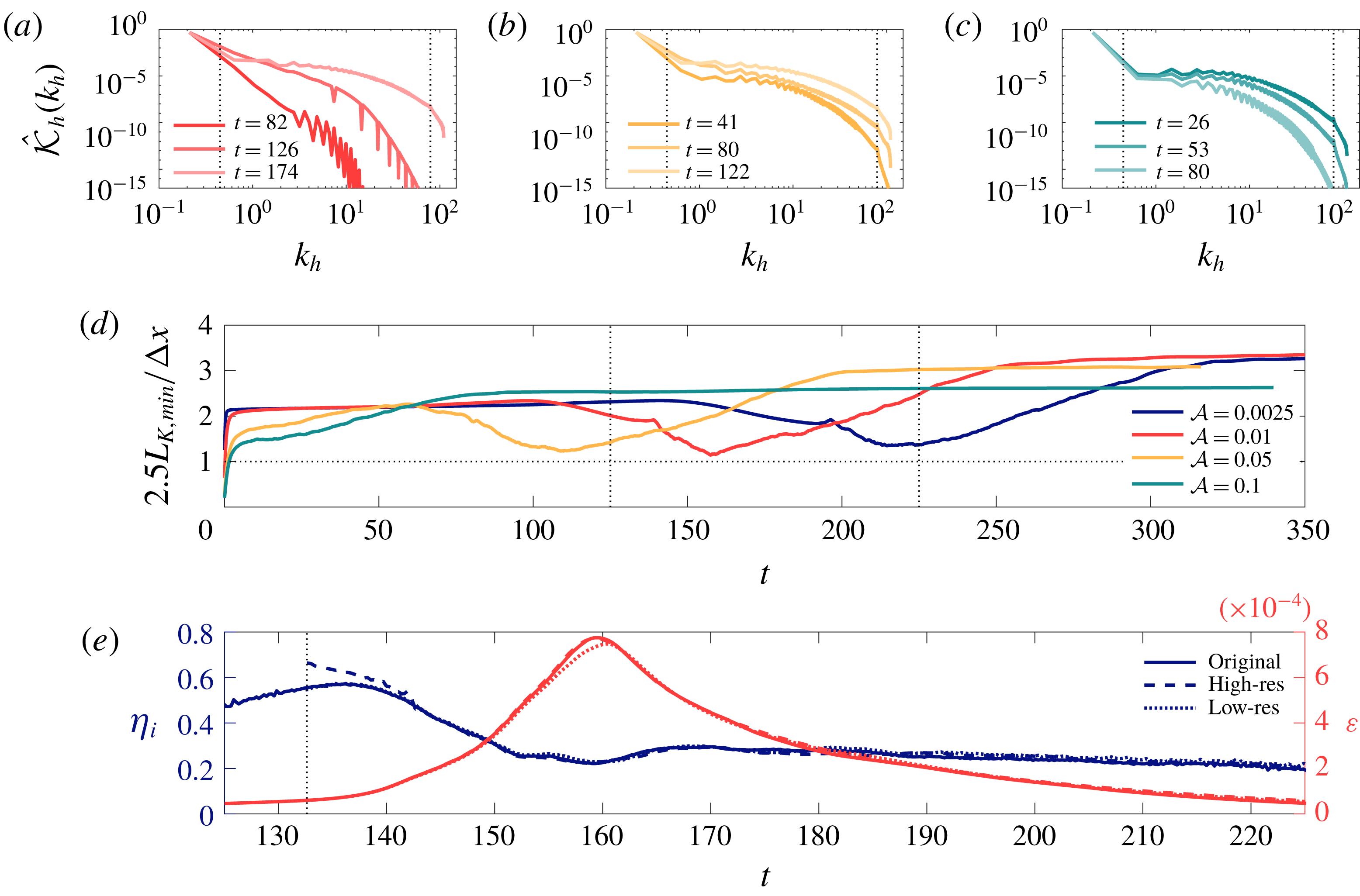
As mentioned in § 2, the grid sizes for our simulations are chosen with the aim of resolving
 $2.5L_{K}$
. However, as discussed in a recent review of mixing efficiency (Gregg et al.
Reference Gregg, D’Asaro, Riley and Kunze2018), inadequate numerical resolution may impact the computed efficiency. In light of this, it is worth revisiting our choice of grid spacing.
We can quantify the amount of energy at various length scales by considering horizontal spectra of kinetic energy,
 $\hat{{\mathcal{K}}}_{h}$
(computed by taking the Fourier transform of
 $\boldsymbol{u}\boldsymbol{\cdot }\boldsymbol{u}$
in the
 $x$
and
 $y$
directions and then averaging in the
 $z$
direction). Figure 8(a–c) show
 $\hat{{\mathcal{K}}}_{h}$
at several times corresponding to the panels in figure 2. The amount of energy contained at the highest wavenumbers is quite small, suggesting that the flow is well resolved in our simulations. Interestingly, figure 8(a–c) is also consistent with the qualitative evolution of the flow shown in figure 2, with elevated energy at small scales when the shear layer is fully turbulent and more energy at the lowest wavenumbers during billow growth.
(a–c) Horizontal spectra of kinetic energy for cases with
 $Re=2000$
and
 $Ri_{b}=0.16$
at several times shown in figure 2. Panels (a), (b) and (c) correspond to
 ${\mathcal{A}}=0.01$
,
 $0.05$
and
 $0.1$
, respectively. Vertical dotted lines denote the Kelvin–Helmholtz wavenumber and the wavenumber associated with the grid spacing. (Note that there is still some energy at higher wavenumbers, corresponding to small three-dimensional scales with high
 $k_{x}$
and
 $k_{y}$
.) (d)
 $2.5L_{K,min}$
scaled by the grid spacing
 $\unicode[STIX]{x0394}x$
for the simulations presented in § 3.1. The horizontal dotted line denotes
 $2.5L_{K}=\unicode[STIX]{x0394}x$
and the vertical dotted lines denote the range of times presented in the bottom panel. (e) Instantaneous mixing efficiency (blue lines) and viscous dissipation (red lines) for simulations with three different grid sizes. The simulations correspond to the case with
 ${\mathcal{A}}=0.01$
,
 $Re=2000$
and
 $Ri_{b}=0.16$
, with the higher- and lower-resolution cases restarted from
 $t\sim 132$
(shown by the vertical dotted line).

In figure 8(d) we compare the minimum Kolmogorov scale in the simulations from § 3.1 (calculated using the maximum value of horizontally-averaged dissipation at each point in time) to our grid spacing. For our chosen grid spacing, we expect
 $2.5L_{K}\geqslant \unicode[STIX]{x0394}x$
. It is clear that, apart from the very early times in the simulation, this condition is achieved. The early transient for the cases with stronger initial turbulence is unavoidable, given that our initial perturbation includes energy at the smallest scales of the flow; however, by
 $t\sim 1$
even the case with
 ${\mathcal{A}}=0.1$
is well resolved.
However, the question remains as to whether a resolution based on
 $2.5L_{K}$
is sufficient. To examine this, we linearly interpolate the full three-dimensional velocity and buoyancy fields onto a grid with coarser resolution,
 $(N_{x},N_{y},N_{z})=(384,128,501)$
, and a grid with finer resolution,
 $(N_{x},N_{y},N_{z})=(768,256,1153)$
. We consider the case with
 $Re=2000$
,
 $Ri_{b}=0.16$
and
 ${\mathcal{A}}=0.01$
, as this is the case with the highest peak dissipation (figure 5
a). We restart these additional simulations at
 $t\sim 132$
, when the primary billow structure has formed and secondary instabilities are beginning to grow.
There is a brief initial transient in the computed mixing efficiency in figure 8(e) for the higher-resolution simulation, related to the use of linear interpolation (which affects the probability distribution function of the buoyancy field and, consequently,
 ${\mathcal{P}}_{b}$
). However, even with this adjustment, there is very little difference at later times in the instantaneous mixing efficiency for either the higher- or lower-resolution cases. In contrast, the viscous dissipation is affected slightly by the grid resolution, with a lower peak value observed for the coarser grid. There is very little difference, however, between
 $\unicode[STIX]{x1D700}$
corresponding to the original simulation and that with the finer grid. The similarity in both
 $\unicode[STIX]{x1D702}_{i}$
and
 $\unicode[STIX]{x1D700}$
between the original and higher-resolution grids therefore shows that the original resolution (determined using
 $2.5L_{K}$
) is sufficient to quantify turbulent mixing in our simulations.