

Introduction
Numerous aqueous environments around metal deposits host fine-scale (cm–μm) laminated metalliferous precipitates, especially in surficial environments, such as surface streams and groundwater. These laminated deposits constitute a record of the fluctuating redox conditions during their formation, which are due to their ephemeral nature and their fluctuations in composition and volume depending on weather events, seasonal variations and/or climate changes (e.g. Shuster et al., Reference Shuster, Rea, Etschmann, Brugger and Reith2018). Biological processes can affect metal-bearing geochemical systems and therefore add to the compositional variability of laminated deposits. Common examples include iron- and sulfur-oxidising bacteria that can catalyse acid-generating geochemical processes (Shuster et al., Reference Shuster, Rea, Etschmann, Brugger and Reith2018), photosynthesising organisms, whose activity can lead to diurnal and seasonal geochemical effects, the effects of temperature fluctuations on metabolism (Alpers et al., Reference Alpers, Nordstrom, Spitzley, Jambor, Blowes and Ritchies2003; Pope et al., Reference Pope, McConchie, Clark and Brown2003; Andrade et al., Reference Andrade, Jamieson, Kyser, Praharaj and Fortin2010) and biomineralisation (Heim, Reference Heim, Reitner and Thiel2011). Consequently, most surficial environments are complex and dynamic biogeochemical systems in which biogenic and geogenic processes control mobilisation and re-precipitation of metals (Reith et al., Reference Reith, Brugger, Zammit, Gregg, Goldfarb, Andersen, DeSantis, Piceno, Brodie and Lu2012a, Reference Reith, Zammit, Pohrib, Gregg and Wakelin2015, Reference Reith, Falconer, Van Nostrand, Craw, Shuster and Wakelin2020).
Biological activity in these environments, particularly that of bacteria, is especially important for mobilising and re-precipitation of metals around mineral deposits (Reith et al., Reference Reith, Rogers, McPhail and Webb2006, Reference Reith, Brugger, Zammit, Gregg, Goldfarb, Andersen, DeSantis, Piceno, Brodie and Lu2012a,Reference Reith, Stewart and Wakelinb, Reference Reith, Brugger, Zammit, Nies and Southam2013, Reference Reith, Zammit, Pohrib, Gregg and Wakelin2015, Reference Reith, Falconer, Van Nostrand, Craw, Shuster and Wakelin2020; Wakelin et al., Reference Wakelin, Anand, Reith, Gregg, Noble and Goldfarb2012a,Reference Wakelin, Anand, Reith, Macfarlane and Rogersb; Sanyal et al., Reference Sanyal, Shuster and Reith2019). Understanding the biologically related processes causing mobility of metals in the surficial environment is important for quantifying environmental issues in the short term (human time scales; Warren and Haack, Reference Warren and Haack2001; Gadd, Reference Gadd2007, Reference Gadd2010; Shuster et al., Reference Shuster, Rea, Etschmann, Brugger and Reith2018). Long-term (geological time scales) biologically mediated metal mobility is also of interest for geochemical exploration of mineral deposits (Reith et al., Reference Reith, Brugger, Zammit, Gregg, Goldfarb, Andersen, DeSantis, Piceno, Brodie and Lu2012a, Reference Reith, Zammit, Pohrib, Gregg and Wakelin2015; Wakelin et al., Reference Wakelin, Anand, Reith, Macfarlane and Rogers2012b). In addition, the precipitates from long-term biologically mediated metal mobility can be significant for mineral processing and resource economics, especially in settings such as supergene alteration (Nordstrom and Southam, Reference Nordstrom, Southam, Banfield and Nealson1997; Enders et al., Reference Enders, Knickerbocker, Titley and Southam2006; Reith et al., Reference Reith, Lengke, Falconer, Craw and Southam2007, Reference Reith, Brugger, Zammit, Nies and Southam2013; Henne et al., Reference Henne, Craw, Gagen and Southam2019a).
This study provides a mainly mineralogical and geochemical overview of some of the biogeochemical systems that have produced laminated metalliferous precipitates in a variety of aqueous environments, from surface streams to the deep ocean, to illustrate the wide variety of laminated deposits. All of our examples form a record of biogeochemical fluctuations over time and have either an inferred or demonstrated biogeochemical component. We document some of the metalliferous similarities in this diverse selection of laminated deposits regardless of their contrasting parageneses, and also highlight some differences. The mineralogical and textural variations that we outline here attest to formation under fluctuating biogeochemical conditions in a complex interplay between biogenic and geogenic processes dominated by geochemical disequilibrium. The micro-scale layering related to varying degrees to biological activity in our examples emphasises the importance of understanding the biogeochemical processes within these microenvironments, and the important role that biogeochemical cycling of metals plays in the solubilisation and mineralisation of metals.
Study context and rationale
Laminated metal deposits through time
Eleven samples were selected (Table 1) that cover a broad range of metalliferous settings and metal combinations. These examples are presented in general order of age, from laboratory experiments (months), through historic mine sites (decades), to supergene weathering and deep-ocean processes (millions to tens of millions of years). Older deposits have fewer constraints on their formation processes and retain less evidence for biological activity. Hence, we combine that limited evidence with inferences from the younger examples to obtain an integrated view of the biogeochemical processes and their metallic residues through time.
Summary of examples of laminated metal deposition from a range of aqueous environments over a range of time scales.

IOB = Fe-oxidising bacteria; IRB = Fe-reducing bacteria; SOB = S-oxidising bacteria; SRB = S-reducing bacteria; MOB= Mn-oxidising bacteria; *Inferred. General references: 1. Henne et al. (Reference Henne, Craw, Gagen and Southam2019a); 2. Kerr and Craw (Reference Kerr and Craw2020); 3. Kerr et al. (Reference Kerr, Craw, Pope and Trumm2018); 4. Alpers et al. (Reference Alpers, Nordstrom, Spitzley, Jambor, Blowes and Ritchies2003); 5. Henne et al. (Reference Henne, Craw, Gagen and Southam2021); 6. Craw and Kerr (Reference Craw and Kerr2017); 7. Reith et al. (Reference Reith, Stewart and Wakelin2012b); Craw et al. (Reference Craw, MacKenzie and Grieve2015); Craw and Lilly (Reference Craw and Lilly2016); 8. Henne et al. (Reference Henne, Craw, Gagen and Southam2019a, Reference Henne, Craw, Gagen and Southam2020); 9. Manceau et al. (Reference Manceau, Lanson and Takahashi2014); Shiraishi et al. (Reference Shiraishi, Mitsunobu, Suzuki, Hoshino, Morono and Inagaki2016); 10. Levett et al. (Reference Levett, Vasconcelos, Gagen, Rintoul, Spier, Guagliardo and Southam2020); Paz et al. (Reference Paz, Gagen, Levett, Zhao, Kopittke and Southam2020); 11. Salama et al. (Reference Salama, Gazley and Bonnett2016).
Samples in this study were selected from material that we obtained in a range of previous studies for entirely different purposes, as outlined in the references in Table 1. These samples were collected from a wide variety of settings associated with mining, exploration and rehabilitation activities and include samples from historic mine waters in the South Island of New Zealand, acid mine drainage in California, USA, anthropogenically neutralised mine drainage in Queensland, Australia, along with samples from oxidised and supergene zones overlaying ore bodies in the South Island of New Zealand, in Salobo, Brazil and Queensland, Australia. In addition, one sample originated from a laterite/soil interface associated with plants over iron ore bodies in Serra Norte, Brazil and one from the North Pacific Ocean floor (manganese nodule). We also include a sample derived from long-term laboratory experiments designed to model the biogeochemical weathering of Cu-bearing lithologies at Salobo, Brazil. These samples, and the near-surface settings from which they were taken, were chosen because they display evidence of fluctuating biogeochemical conditions that have led to laminated deposits. The details of biological and geochemical contributions to formation of these laminated deposits are covered more specifically in references cited herein and other related studies, and some biological aspects of the geologically older material can only be inferred on the basis of the known near-surface settings.
Our chosen examples all show evidence for fluctuating biogeochemical conditions during their formation. We focus on the generalised variations and gradients in redox and pH conditions that have contributed to the formation of these disparate precipitates, and the mineralogical results of these processes. Most of these examples have dominant or primary metals (especially Fe and/or Mn), in which geochemical variations largely control the precipitation processes. These dominant metals are accompanied by other metals that become incorporated into laminated precipitates as a result of secondary or collateral effects.
Theoretical basis for biogeochemical variations
Although biological processes can catalyse chemical reactions that operate within thermodynamic principles, there is an underlying thermodynamic control on the formation of laminated metallic deposits. In the surficial environment, the Gibbs free energy change of a reaction, ΔG reaction, has two components, the standard Gibbs free energy of the reaction, ΔG°reaction, and the reaction quotient, Q:
 $$\Delta G_{{\rm reaction}} = \Delta G^\circ _{{\rm reaction}} + RT\ln Q$$
where R is the gas constant and T is the temperature (~298 K was chosen as an average temperature for the surficial environments modelled in this study). The reaction quotient Q is the ratio of multiplied activities of reaction products and multiplied activities of reactants. At equilibrium, Q is equal to the equilibrium constant, K eq. As ΔG reaction is zero at equilibrium,
 $$\Delta G^\circ _{{\rm reaction}} = \ndash RT\ln K_{{\rm eq}}$$
Combining reactions 1 and 2 yields:
 $$\Delta G_{{\rm reaction}} = RT\lpar {\ln Q\ndash lnK_{{\rm eq}}} \rpar $$
Hence, when Q < K eq the reaction goes forward, and when Q > K eq the reaction is reversed. The special condition of equilibrium is relatively rare in dynamic surficial environments. Bacteria, in particular, can use enzymes to gain energy for metabolic processes that catalyse reactions from a disequilibrium state where Q < K eq and thereby can accelerate the rate at which reactions progress towards equilibrium (Q = K eq) (Deamer and Weber, Reference Deamer and Weber2010).
As an example, one of the most common reactions in the surficial environment is the relationship between dissolved ferrous iron and ferrihydrite:
 $${\rm F}{\rm e}^{2 + } + 0.25{\rm O}_2 + 2.5{\rm H}_2{\rm O} \to {\rm Fe}\lpar {{\rm OH}} \rpar _3 + 2{\rm H}^ + $$
The reaction quotient is:
 $$Q_{{\rm ferrihydrite}} = \lsqb {\rm H}^ + \rsqb ^2/\lpar \lsqb {\rm F}{\rm e}^{2 + }\rsqb \lpar {{\rm p}{\rm O}_2} \rpar ^{0.25}\rpar $$
where pO2 is the partial pressure of oxygen. Therefore, the ferrihydrite reaction (4) is dependent on pH, oxygen partial pressure or redox conditions, and the amount of dissolved ferrous iron. While temperature can be an important variable within surficial environments, here we focus on fluctuations of the three variables above, as they are common in surficial environments for a wide range of biogeochemical reasons, as outlined below. Consequently, disequilibrium dissolution and/or precipitation of iron (and other metals) is a widespread biogeochemical phenomenon, as in many of the examples in Table 1 that are described below.
Methods
Mineralogy and textures for most samples have been characterised using polished thin sections, light microscopy, X-ray diffraction (XRD) and synchrotron X-ray fluorescence microscopy (XFM). More detailed textural and geochemical observations were made using scanning electron microscopy (SEM) with energy dispersive X-ray spectroscopy (EDS) on polished thin sections and freshly-broken surfaces. Details regarding SEM instrument parameters and settings are given in Kerr et al., (Reference Kerr, Craw, Pope and Trumm2018) and Henne et al., (Reference Henne, Craw, Gagen and Southam2019a, Reference Henne, Craw, Gagen and Southam2020).
Synchrotron X-ray fluorescence microscopy was used on selected samples to obtain relative element-distribution maps of transition metals, with detection limits of ~100 ppm. The XFM maps were generated on the XFM beamline (Paterson et al., Reference Paterson, de Jonge, Howard, Lewis, McKinlay, Starritt, Kusel, Ryan, Kirkham, Moorhead and Siddons2011) at the Australian Synchrotron, ANSTO. The maps were generated using a monochromatic X-ray beam at 18,500 eV, focussed using Kirkpatrick–Baez mirrors to ~2 μm with a dwell per pixel of 0.2 to 0.5 msec. Data were collected with a Maia detector (Ryan et al., Reference Ryan, Siddons, Kirkham, Dunn, Kuczewski, Moorhead, De Geronimo, Paterson, de Jonge, Hough, Lintern, Howard, Kappeng and Cleverleya2010, Reference Ryan, Siddons, Kirkham, Li, de Jonge, Paterson, Kuczewski, Howard, Dunn, Falkenberg, Boesenberg, De Geronimo, Fisher, Halfpenny, Lintern, Lombi, Dyl, Jensen, Moorhead, Cleverley, Hough, Godel, Barnes, James, Spiers, Alfeld, Wellenreuther, Vukmanovic and Borg2014), and full spectrum data (sensitive to elements from Sr to Zr) were analysed using the GeoPIXE software program (Ryan, Reference Ryan1999). X-ray fluorescence microscopy element data are derived from irradiation of the entire thickness (~30 μm) of the polished section, so the technique cannot resolve sub-μm particles amongst underlying and/or overlapping particles.
In addition, the X-ray absorption near edge spectroscopy (XANES) mapping capability of the XFM beamline was used to investigate Cu speciation within regions of interest that were selected from element-distribution maps of selected samples. Copper K-edge XANES analysis was undertaken over the energy range of 8900 to 9300 eV, with maximum energy steps of 25 eV in the post-edge region (9100 to 9300 eV), and minimum energy steps of 0.5 eV over the edge (8976 to 9000 eV). Spectra were collected across regions of interest with a step size of 4–5 μm. Dwell times varied between samples within the range of 0.5 to 5 msec per pixel. The reference materials used as standards for comparison were native copper tape, Cu(I) chloride, Cu(I) oxide, Cu(II) chloride, Cu(II) oxide, Cu(II) carbonate and Cu(II) sulfate. GeoPIXE was used to process the data before Athena software was used for background subtraction and normalisation (Ravel and Newville, Reference Ravel and Newville2005).
Descriptions of laminated metalliferous deposits in different aqueous environments
Laminated precipitates in laboratory weathering experiments
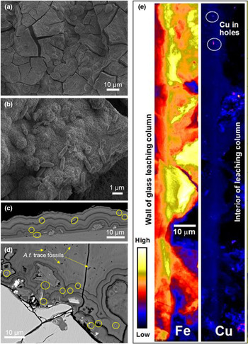
In laboratory-scale weathering experiments of fresh rocks from the Salobo iron-oxide copper–gold (IOCG) deposit in Brazil, finely laminated metalliferous precipitates were produced within ~400 days in a biogeochemical system dominated by Acidithiobacillus ferrooxidans, an acidophilic, iron-oxidising bacterium (Henne et al., Reference Henne, Craw, Vasconcelos and Southam2018, Reference Henne, Craw, Gagen and Southam2019a, Reference Henne, Craw, Gagen and Southam2020). These experiments were conducted in small-scale (10 cm3) polypropylene columns, partially filled with crushed, weakly mineralised rock. The rocks were dominated by iron-bearing silicates with minor disseminated chalcopyrite and bornite. A strain of A. ferrooxidans was cultured from the Salobo mine site and used for the experiments, as described by Henne et al. (Reference Henne, Craw, Vasconcelos and Southam2018, Reference Henne, Craw, Gagen and Southam2019a,Reference Henne, Craw, Gagen and Southamb, Reference Henne, Craw, Gagen and Southam2020). Samples of the column solutions (2 mL) were obtained every two days and replaced with fresh growth medium to sustain active metabolic activity of bacteria. After completion of the experiments, some columns were opened to view the precipitates that had formed on rock clasts (Fig. 1a,b). Some columns were embedded in situ, sectioned, and polished for examination by light microscopy, SEM and XFM (Fig. 1c,d,e; Henne et al., Reference Henne, Craw, Gagen and Southam2019a, Reference Henne, Craw, Gagen and Southam2020).
Laminated precipitates formed in laboratory-based biogeochemical weathering experiments. (a) General SEM view of ferrihydrite precipitate with dehydration cracks from sample preparation on a rock clast. (b) Cells of A. ferrooxidans on ferrihydrite precipitate. (c) Back-scattered electron image of a section through ferrihydrite precipitate coating the wall of a leaching column with trace fossils of A. ferrooxidans (yellow circles). (d) Back-scattered electron image of a section through laminated ferrihydrite precipitate with trace fossils of A. ferrooxidans (yellow circles and arrows) on a chalcopyrite clast. (e) XFM element-distribution maps for Fe and Cu of laminated ferrihydrite precipitate on the wall of the experimental vessel. Enhanced Cu deposition at bacterial trace fossils are indicated (white circles).

Secondary precipitates that formed around some particles and on the walls of the columns were dominated by ferrihydrite (Fe[OH]3; although this material was largely amorphous). Some of the precipitates exhibited fine (micrometre-scale) laminations reflecting differing degrees of hydration, chemical composition, and different nanoparticulate particle sizes. These laminations followed the relief of the substrate as well as abundant micrometre-scale circular holes that were trace fossils of individual A. ferrooxidans cells, permineralised in situ during deposition of acicular ferrihydrite (Fig. 1c,d). In general, the distribution of Cu followed the deposition of ferrihydrite laminations, which contained up to 7 wt.% Cu. Interestingly, Cu content was elevated locally within bacterial trace fossils (Fig. 1e).
Laminated precipitates in historic mine wastes
Laminated precipitates found in historic mine wastes, which were abandoned without rehabilitation, provide an opportunity to observe results of biogeochemical processes over human time scales. These laminations record changes in biogeochemical conditions during surficial weathering processes, which influence metal mobility. In two examples from orogenic gold deposits in New Zealand (Waiuta mine and Macraes mine; Fig. 2a–d; Table 1), metals have been dissolved and redeposited by shallow groundwater, forming precipitates that cement the waste materials (Fig. 2a–d). These cementation processes are affected by the weather and seasonal variations that are imposed on inhomogeneous materials that will inevitably include biological components. The constantly changing groundwater compositions result in laminated precipitates reflecting this wide range of biogeochemical conditions. The ore, and subsequent tailings, from these mines contained abundant arsenic (As). The ambient pH at both sites was circumneutral because of ample carbonate in the rocks, but processing of the ore and subsequent weathering has resulted in localised acidification within the tailings deposits (Table 1).
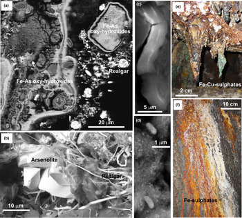
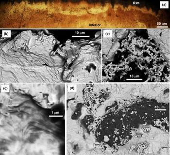
Laminated precipitates formed at historic mines. (a) SEM view of cemented tailings on a wood fragment; Waiuta orogenic gold mine, New Zealand. Laminated As-bearing Fe-oxyhydroxide precipitates (mid-grey) coat some of the clasts, with an outer layer of realgar (AsS; bright white) precipitate. (b) Magnified view of the same deposit as in (a), showing arsenolite crystals (As2O3) with overgrowths of hair-like realgar. (c) SEM view of As–Hg-bearing ferrihydrite cement in historic tailings from Macraes orogenic gold mine, New Zealand, in which Hg was used for gold extraction. The cement is laminated with differing proportions of As and different Hg contents are shown as brighter and darker layers. (d) Magnified view of the same deposit as in (c), showing precipitate lamina rich in schuetteite (Hg3[SO4]O2) and possibly preserved bacterial cells partially per-mineralised by schuetteite. Some of the smallest white dots are nanoparticulate liquid Hg droplets. (e) Photograph of laminated precipitates forming stalactites on the roof of an underground tunnel, Iron Mountain mine, California. (f) Photograph of laminated precipitates on the wall of the mine in (e).

Tailings from the Waiuta mine have been cemented variably by As minerals with a wide range of oxidation states, and these different minerals occur in close proximity at the micrometre-scale (Fig. 2a,b). These tailings were deposited in a shallow (~10 m) depression that has been water-saturated for >80 years and subjected to regular heavy rain events in a wet climate (rainfall >2000 mm/year). The deposit hosts abundant organic matter, including mosses, algae and bacteria, and some woody material from the surrounding rainforest (Kerr et al., Reference Kerr, Craw, Pope and Trumm2018). The most chemically-reduced cementing mineral, realgar, occurred principally on decomposing wood fragments within the tailings (Fig. 2a,b). This setting has resulted in extreme and fluctuating biogeochemical redox gradients within the tailings, leading to laminated precipitates that range from highly oxidised to highly reduced (Fig. 2a,b).
In contrast, the historic tailings from the Macraes mine have been weathering in a semiarid climate (rainfall ~600 mm/year) for ~80 years with associated evaporation facilitating formation of dry, hard, As-bearing ferrihydrite cement (Fig. 2c,d). Carbonaceous debris and relict sulfide minerals within the tailings have facilitated formation of small scale (micrometre to millimetre) redox gradients within the thin (<1 m) cemented deposit that is fully exposed to seasonal weather variations ranging from hot summers (>30°C days) to cold winters (<10°C nights). Historically, mercury amalgamation was used for gold extraction, and some remnants of this Hg remain in the tailings as liquid Hg droplets and as the more oxidised mineral schuetteite (Fig. 2c,d). Mercury has been incorporated variably into the ferrihydrite cement, forming distinct laminations (Fig. 2c,d). Liquid mercury droplets coexist with, and have locally formed on, schuetteite precipitates, and vice versa (Fig. 2d), reflecting the variable and fluctuating redox gradients in the tailings. Partially permineralised bacterial cells (Fig. 2d) attest to a biological component of the cementation processes.
Laminated precipitates from acid mine drainage
Aqueous environments affected by acid mine drainage (AMD) commonly host laminated deposits (Shuster et al., Reference Shuster, Reith, Izawa, Flemming, Banerjee and Southam2017, Reference Shuster, Rea, Etschmann, Brugger and Reith2018). Acid mine drainage results from discharge of shallow groundwater that has been affected by oxidation of sulfide minerals (especially pyrite) that have been exposed by mine excavations. From a biogeochemical perspective, sulfide oxidation is facilitated invariably by a wide range of bacterial species involving various reactions (Baker and Banfield, Reference Baker and Banfield2003; Johnson and Hallberg, Reference Johnson and Hallberg2005; Dold, Reference Dold2014; Quatrani and Johnson, Reference Quatrini and Johnson2018). The historic Iron Mountain underground mine in California, USA (Fig. 2e,f; Table 1) is one of the most spectacular examples of AMD in the world where laminated metalliferous precipitates have formed. At the Iron Mountain underground mine, bacterially mediated oxidation reactions generated underground waters with a pH that ranges down to negative values (Alpers et al., Reference Alpers, Nordstrom, Spitzley, Jambor, Blowes and Ritchies2003). The resulting AMD compositions change on time scales of seasons to years (Alpers et al., Reference Alpers, Nordstrom, Spitzley, Jambor, Blowes and Ritchies2003) and precipitates are laminated accordingly (Fig. 2e,f). Most of the precipitates are dominated by ferrous and ferric sulfate minerals (Fig. 2e,f), reflecting the very high dissolved sulfate concentrations in the AMD and fluctuating redox conditions (Alpers et al., Reference Alpers, Nordstrom, Spitzley, Jambor, Blowes and Ritchies2003). In addition, variable amounts of Cu and Zn sulfate minerals contributed to the laminated precipitates (Fig. 2e).
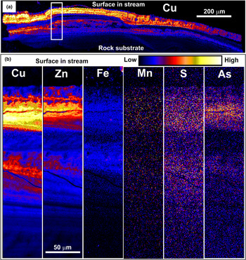
In an example of pH neutral surface waters at the Cu–Au mine at Mt Chalmers, Queensland, Australia (Table 1), AMD derived from tailings and relict mine walls have been neutralised with alkaline waste rock. Treatment of AMD discharges from historic mines is becoming common practice at many sites to ameliorate the downstream environmental effects. Treatment typically involves raising the pH using an acid-consuming material. The neutralisation of discharging waters at Mt Chalmers, which initially had a low pH (<4) and very high Cu and Zn concentrations, caused Cu and Zn sulfate precipitation on downstream cobbles. Precipitates are locally intergrown with biofilms, creating spectacularly laminated metalliferous deposits (Fig. 3a,b). The biofilms contain a wide variety of bacteria and archaea, some of which are photosynthetic, as well as moss, algae and macroinvertebrates. Some parts of the biofilms also include fossilised fragments of eukaryotes that have enhanced localised Cu and Zn deposition (Henne et al., Reference Henne, Craw, Gagen and Southam2021).
XFM element-distribution maps of a thin section through laminated mineral precipitates on a biofilm growing on a cobble downstream of the treated AMD at the Mt Chalmers Cu–Au mine, Australia. (a) General view of Cu contents in the laminated deposit. (b) Magnified view of the portion indicated in (a), showing relative concentrations of Cu, Zn, Fe, Mn, S and As.

Laminated precipitates from supergene weathering and oxidation
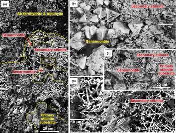
Laminated metalliferous precipitates, formed during incipient weathering of sulfide-bearing deposits, record the steep redox gradient between the primary sulfides and the most oxidised exterior minerals exposed to the atmosphere and/or oxygenated groundwater. Our example from an orogenic gold deposit from New Zealand (Table 1) of this type of redox gradient is on primary stibnite (Fig. 4a–d). The sulfides of the deposit have been exposed at the surface by erosion on a steep mountainside, and a thin (<1 m) zone of variably oxidised metallic secondary minerals has formed, with minimal metal mobility as transformations occurred largely in situ. The secondary minerals have a complex paragenesis of mutual overgrowths in crude layering within the redox gradient (Fig. 4a–d). The most oxidised veneer consists of Sb-bearing ferrihydrite and tripuhyite, and variably distributed senarmontite and secondary stibnite have formed in between the oxidised veneer and the primary stibnite (Fig. 4a). The senarmontite locally overgrows secondary stibnite and is locally overgrown by the secondary stibnite (Fig 4b–d). The secondary stibnite has a distinctive tubular texture with a high surface area reminiscent of permineralised filamentous bacteria, indicating a biological influence on formation (Fig. 4d).
SEM images of laminated secondary Sb minerals developed in an oxidised Au–As–Sb orogenic deposit, Otago Schist, New Zealand. (a) General view of contrasting redox minerals developed on primary stibnite (bottom), with secondary stibnite beneath Sb-bearing ferrihydrite and tripuhyite (FeAsO4). (b, c) Magnified view of secondary minerals in the redox gradient in (a), with secondary stibnite overgrowing secondary senarmontite crystals (Sb2O3). (d) Magnified view of secondary stibnite, showing a tubular morphology produced potentially by filamentous bacteria.

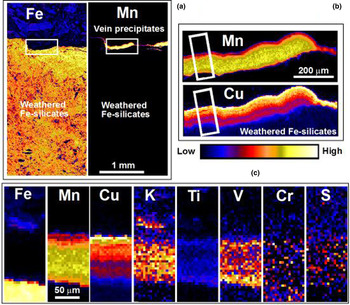
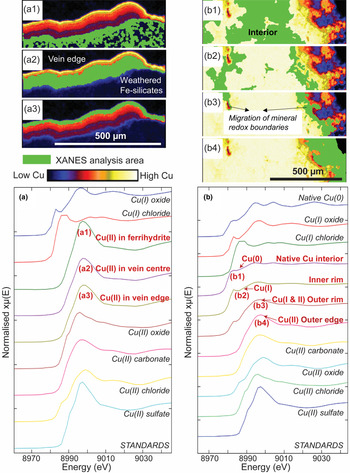
More advanced weathering and oxidation was observed in our example from the saprolitic zone developed on the Precambrian Salobo IOCG deposit of Brazil (Fig. 5a–c; Table 1). This led to the development of a subsurface saprolitic zone in which the rocks have been oxidised extensively and variably altered to clays. This oxidation and alteration was driven partly by a wide range of bacteria, including Fe-, Mn- and S-oxidisers and Fe-reducers, that occur within water-saturated fractures exposed by the mine excavation (Henne et al., Reference Henne, Craw, Gagen and Southam2020). In this saprolitic zone, typically more extensive metal mobility has occurred than in the previous incipient weathering example, and metal-bearing veins can form in structurally controlled sites. The example from the saprolitic zone developed at Salobo consists of a delicately laminated Cu- and Mn-rich vein that has formed on a fracture surface in a rock dominated by weathered Fe-silicates (Fig. 5). Although there is abundant Fe in the general environment, there is only minor Fe in the vein (<1 wt.%; Fig. 5a,c). However, the vein includes a wide range of other elements in addition to the dominant Cu and Mn (Fig. 5c). Synchrotron-based XANES (Fig. 6a) revealed that Cu within the vein material, and the relatively low levels within the ferrihydrite substrate, occurred as Cu(II).
XFM element-distribution maps of a thin section through a laminated vein formed during weathering of the Salobo IOCG deposit, Brazil. (a) Fe and Mn maps show the location of the vein (Mn rich) on the margin of oxidised rock (Fe rich). (b) Magnified view of the vein (as indicated in (a) showing laminae enriched in Mn and Cu. (c) Juxtaposed elemental sections through the vein, as indicated in (b).

Regions of interest from which Cu XANES spectra are extracted are numbered and highlighted in green, and are shown against a background map of Cu K-edge fluorescence intensity at 9.3 keV. A range of Cu(0), Cu(I) and Cu(II) standards are shown for comparison. (a) Spectra from the laminated vein and its substrate in saprolite from the Salobo mine (Fig. 5). (b) Spectra from the interior, inner and outer rim zones, and outer edge of the native copper sample from Mt Isa (Fig. 7).

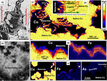
A common component of supergene weathering zones on copper-rich mineral deposits is native copper, which typically forms in the lower (more reduced) portions of an overall redox gradient in these zones. The example we depict in Fig. 7a–d is from the saprolitic weathering zone on the Precambrian rocks of the Mt Isa inlier in Queensland, Australia (Table 1). Weathering and progressive oxidation have resulted in the formation of a laminated rim zone around the mass of native copper (Fig. 7a–d). The redox gradient and associated mineralogy are similar to that of the supergene zone over the Salobo deposit in which we have abundant evidence for bacterial involvement (previously described above), and the Fe-oxyhydroxide minerals associated with native Cu grains in the Mt Isa samples display the acicular texture typical of Fe-oxyhydroxide precipitates facilitated by Fe-oxidising bacteria (Loiselle et al., Reference Loiselle, McCraig, Dyar, Léveillé, Shieh and Southam2018) and bacterially sized moulds within these precipitates (Fig. 7a,b). The outermost part of the native copper rim zone consists of crystalline malachite (Fig. 7c–f) that is readily identifiable in hand specimen and is clearly a Cu(II) mineral in XANES analysis (Fig. 6b). The innermost portion of the rim zone shows up in incident light microscopy and XFM mapping as a diffuse zone that is different texturally from both the outermost crystals and the native Cu interior (Fig. 7d,e). This inner rim is shown by XANES analysis (Fig. 6b) to contain Cu(I) and is presumed to be cuprite. Iron is confined to the outer layers (Fig. 7e,f), and some relatively Fe-rich parts of this layer contain arsenic, possibly as scorodite (Fig. 7f).
SEM images and XFM element-distribution maps of laminations observed in supergene samples from Mt Isa, Queensland, Australia. (a) Back-scattered electron image of a cross-section through Fe-oxyhydroxides in native-copper-bearing rocks organised in colloform textures. (b) Potential bacteria fossil remnant in Fe-oxyhydroxide with acicular texture. (c) Copper XFM map of laminated rims on a supergene native copper nugget. (d) Magnified view of the rim zone in (a), showing principal minerals. (e) Paired Cu and Fe XFM maps of rim layers. (f) Copper, Fe and As XFM maps of rim layers. The As map has high background from the mounting glass, which obscures a zone of As enrichment that follows the outer edge.

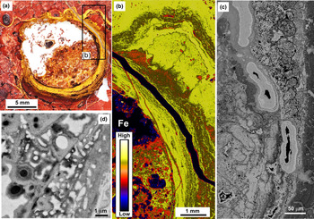
At the interface of saprolitic rock and lateritic soil, more advanced oxidation during weathering and progressive leaching of mobile metals can leave a goethite-cemented zone known variously as ferricrete, duricrust, or canga (Gagen et al., Reference Gagen, Levett, Paz, Gastauer, Caldeira, Valadares, Bitencourt, Alves, Oliveira, Siqueira, Vasconcelos and Southam2019; Levett et al., Reference Levett, Vasconcelos, Gagen, Rintoul, Spier, Guagliardo and Southam2020; Paz et al., Reference Paz, Gagen, Levett, Zhao, Kopittke and Southam2020). In our samples of canga over a supergene Fe deposit near the Serra Norte mine in Brazil (Table 1), deposits of Fe-oxyhydroxides dominated by goethite form a hard surface crust to the landscape. Native sedges (Cyperaceae) grow in rupestrian grasslands on the canga and extend their roots into the Fe-rich substrate (Fig. 8a). Biogeochemical processes have led to the formation of laminations with varying proportions of Fe-oxyhydroxides at a range of scales: around centimetre root channels (Fig. 8a,b), and in smaller root-related cavities (tens of μm; Fig. 8c). Microorganisms are preserved extensively as permineralised fossils in goethite-rich bands around root channels in our samples (Fig. 8c,d). The biogeochemical processes also mobilised and reprecipitated some aluminium as part of the microlaminated deposits in the rhizosphere (Fig. 8a–d), typically as gibbsite (e.g. Levett et al., Reference Levett, Gagen, Diao, Guagliardo, Rintoul, Paz, Vasconcelos and Southam2019).
Lamination in an empty root channel in canga from Serra Norte, Brazil. (a) Photograph of a horizontal cross-section with laminations inside a root channel, with (b) corresponding iron distribution from XFM. (c) Back-scattered electron image of various Fe-oxyhydroxide bands in cavities and infilling cracks. (d) Back-scattered electron image of laminations composed of per-mineralised fossils and encrusted cells enveloped by partially Al-substituted goethite.

Laminated precipitates developed during surficial gold mobility and redeposition
Laminated rims around gold particles, such as in our example from the Otago Schist terrane, New Zealand (Table 1; Fig. 9) are common in alluvial gold particles. Gold is locally mobile within supergene alteration zones and in near-surface sedimentary environments (Fig. 9a–e). Though some local Au enrichment does occur, most Au mobility results in increases in some particle sizes at the expense of other smaller particles nearby. As a consequence, gold particles can show evidence for this particle size increase as laminated rims (Fig. 9a). Supergene nuggets are commonly crystalline, and stacked layers of crystalline gold in the rim zones attest to the progressive addition of gold in the near-surface environment (Fig. 9b,c). In addition, more irregular, commonly vermiform gold overgrowths occur on both supergene nuggets, and on detrital gold particles. There is abundant evidence that gold overgrowths at the 1 to 50 μm scale have a biological component to their origins (Reith et al., Reference Reith, Lengke, Falconer, Craw and Southam2007, Reference Reith, Falconer, Van Nostrand, Craw, Shuster and Wakelin2020; Kerr and Craw, Reference Kerr and Craw2017). The role of direct biological processes in the growth of larger nuggets is more controversial. However, biological activity such as bacterial decomposition of primary sulfide minerals in supergene zones has an indirect effect on the biogeochemical processes of Au mobility by generating metastable thiosulfate ions that can complex with Au (Shuster et al., Reference Shuster, Bolin, MacLean and Southam2014).
Layering on the margins of gold particles from the Otago Schist terrane, New Zealand. (a) Incident light view of laminated rim of a supergene gold nugget. (b) SEM view of layered crystalline gold on the margin of a supergene nugget. (c) Magnified view of crystalline gold laminations in (b). (d) Vermiform gold overgrowths on an alluvial gold particle close to the bedrock supergene source. (e) Magnified view of vermiform gold overgrowth in (d).

Laminated precipitates forming manganese nodules
Manganese nodules occur on the deep ocean floor where very low sedimentation rates allow biogeochemical processes to contribute to localised metal accumulation. These nodules precipitate from metals that are mobilised from underlying abyssal sediments and metals that precipitate directly from the surrounding water, and have spectacular laminated structures (Fig. 10). Nodules have been investigated extensively as potential sources of metal resources, so geochemical, mineralogical and biological features have been well established (Hein et al., Reference Hein, Mizell, Koschinsky and Conrad2013; Hein and Kaschinsky, Reference Hein and Koschinsky2014; Manceau et al., Reference Manceau, Lanson and Takahashi2014; Shiraishi et al., Reference Shiraishi, Mitsunobu, Suzuki, Hoshino, Morono and Inagaki2016; Benites et al., Reference Benites, Millo, Hein, Nath, Murton, Galante and Jovane2018). Here we summarise conclusions from these authors and references therein to provide a context for our general observations on the well-developed metallic laminations in our sample from the North Pacific Ocean that we depict in this paper (Fig. 10).
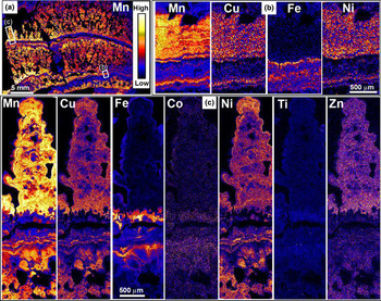
XFM element-distribution maps showing laminations in a manganese nodule from the North Pacific Ocean floor. (a) General view of Mn distribution in a polished section through the nodule. (b) Magnified view of a strip through (a), showing Mn, Cu, Fe and Ni distributions in a combination of primary laminations and secondary (diagenetic) layers that truncate the primary laminae and locally obscure them. (c) XFM element-distribution maps showing a detailed view of primary metallic laminations of Mn, Cu, Fe, Co, Ni, Ti and Zn in an individual protrusion.

Manganese nodules are dominated by Mn oxides and Fe oxides, with incorporation of a range of other transition metals, particularly Cu, Co and Ni. Some primary depositional parts of the nodules undergo diagenetic transformations of mineralogy and texture, accompanied by redistribution of metals. While recent research indicates that the mobility of metals is probably linked to the structural properties of the hosting Mn oxide (Wu et al., Reference Wu, Peacock, Lanson, Yin, Zheng, Chen, Tan, Qiu, Liu and Feng2019), the specific minerals and metals that occur in various laminations in the nodules are also controlled by localised redox gradients that occur near to the nodule-sediment interface and the resulting diagenetic processes. Redox gradients and associated chemical activity are partially controlled by biological agents, particularly bacteria and archaea in the sediments and on the nodule surfaces. Biological processes can also facilitate localised changes in pH to more acidic conditions that differ from the ambient pH ≈ 8 of surrounding seawater. Importantly, the redox and pH gradients change with time as a result of variations in environmental factors, such as currents and changing supply of decomposing organic material. Consequently, the delicately laminated nodules record accumulation and transformation in situ in an environment of slow biogeochemical cycling. In our sample, there was a general separation of Mn and Fe deposition during these processes, although they were not entirely mutually exclusive (Fig. 10b,c). Likewise, other metals are generally enriched with Mn rather than Fe, but some metal-enriched Fe laminae also occur (Fig. 10b,c).
Discussion
Formation of iron-rich laminations
Iron dissolution and precipitation in surficial environments is controlled largely by reactions 4 and 5 (above). The oxygen partial pressure in many surficial environments is very low and is commonly quantified instead by redox reactions that lead to the use of Eh–pH diagrams to depict the relationships in reactions 4 and 5 (Fig. 11a). Changes in the variables in reaction 5 result in changes in the relative proportions of ferrihydrite and dissolved Fe2+. Boundaries on the Eh–pH diagram (Fig. 11a) depict the combinations of the three variables in Q that lead to chemical equilibrium. The three variables in reaction 5 typically change widely in surficial environments as a result of biogeochemical processes, and disequilibrium is the norm. For example, oxidation at constant pH and [Fe2+] favours ferrihydrite precipitation, and reduction reverses this reaction (Fig. 11a). Conversely, acidification at constant pO2 and [Fe2+] will dissolve ferrihydrite, but neutralisation will cause ferrihydrite reprecipitation (Fig. 11a).
Eh–pH diagrams (from Geochemist's Workbench, Bethke and Yeakel, Reference Bethke and Yeakel2016) showing redox relationships for Fe species in surficial environments. Heavy arrows indicate typical environmental fluctuations that lead to laminated precipitates. (a) Simple system with equilibrium lines for reaction 4 (in text) for a range of dissolved Fe2+. (b) A high-sulfate system depicting fluctuations in AMD environments.

All three variables in Q in the ferrihydrite reaction (4) are likely to change at the same time as a result of biotic and/or abiotic processes, and it is these types of fluctuations that lead to the widespread layering observed in the precipitates in our examples of laminated deposits from laboratory weathering of Cu-bearing rocks (Fig. 1), and natural samples from the supergene zones at the Salobo IOCG mine in Brazil (Figs 5, 6) and the Mt Isa mine in Australia (Fig. 7). Iron oxidation via reaction 4 generates hydrogen ions, and this can lead to acidification within the rocks (Singer and Stumm, Reference Singer and Stumm1970; Langmuir, Reference Langmuir1997; Dockrey et al., Reference Dockrey, Lindsay, Mayer, Beckie, Norlund, Warren and Southam2014). Initial oxidation of ferrous to ferric iron is kinetically very slow under acidic conditions (time scales of years to centuries; Langmuir, Reference Langmuir1997). However, bacterial mediation of the reaction can increase this rate by orders of magnitude and make it essentially instantaneous (Singer and Stumm, Reference Singer and Stumm1970; Langmuir, Reference Langmuir1997; Henne et al., Reference Henne, Craw, Gagen and Southam2019a). If the overall biogeochemical environment has a circumneutral pH and some inherent neutralising capacity, this bacterially mediated acidification may be confined to the mineral grain scale where the oxidation is focussed (Langmuir, Reference Langmuir1997; Mielke et al., Reference Mielke, Pace, Porter and Southam2003; Dockrey et al., Reference Dockrey, Lindsay, Mayer, Beckie, Norlund, Warren and Southam2014; Henne et al., Reference Henne, Craw, Vasconcelos and Southam2018, Reference Henne, Craw, Gagen and Southam2019a,Reference Henne, Craw, Gagen and Southamb) and result in micrometre-scale laminations at grain boundaries. Laminated precipitates in Figs 1a–e and 7e,f reflect these micrometre-scale, biologically mediated, localised variations in pH within bulk circumneutral pH. Precipitation of metal-rich laminations from the abandoned Mt Chalmers mine site in Australia depicted in Fig. 3b was driven by anthropogenic addition of neutralisation capacity with moss and algae as the substrate for precipitation. Laminations within this sample probably also reflect fluctuations in water availability linked to periods of rainfall and evaporation (Henne et al., Reference Henne, Craw, Gagen and Southam2021), which can dilute or concentrate metals in solution and affect microbial populations that rely on water.
In our example of laminated deposits in plant root cavities at Serra Norte, Brazil (Fig. 8), organic acid production in the plant rhizosphere results in localised variations in pH and redox states in lateritic soils (Gagen et al., Reference Gagen, Levett, Paz, Gastauer, Caldeira, Valadares, Bitencourt, Alves, Oliveira, Siqueira, Vasconcelos and Southam2019; Paz et al., Reference Paz, Gagen, Levett, Zhao, Kopittke and Southam2020). These biogeochemical changes, combined with associated bacterial activity, have resulted in differential Fe mobilisation and reprecipitation (Fig. 8a–d; Gagen et al., Reference Gagen, Levett, Paz, Gastauer, Caldeira, Valadares, Bitencourt, Alves, Oliveira, Siqueira, Vasconcelos and Southam2019; Paz et al., Reference Paz, Gagen, Levett, Zhao, Kopittke and Southam2020; Levett et al., Reference Levett, Vasconcelos, Gagen, Rintoul, Spier, Guagliardo and Southam2020). The variable amounts of Al accompanying Fe in these laminations was mobilised as a trivalent ion and behaves in a geochemically similar manner to ferric iron and precipitates under circumneutral pH conditions (Fig. 11b). In addition, trace metals such as Co, Cr, Mn, Ti and V have been mobilised in the rhizospheric setting to form larger-scale (multiple millimetres) metal-rich laminations similar to those that occur at deeper levels (Fig. 5c), although in the surficial lateritic environment these trace metals are associated closely with Fe-oxyhydroxides (Gagen et al., Reference Gagen, Levett, Paz, Gastauer, Caldeira, Valadares, Bitencourt, Alves, Oliveira, Siqueira, Vasconcelos and Southam2020).
In environments with less inherent neutralising capacity, bacterially mediated oxidation processes can generate larger-scale AMD (Alpers et al., Reference Alpers, Nordstrom, Spitzley, Jambor, Blowes and Ritchies2003; Lottermoser, Reference Lottermoser2010; Parbakhar-Fox and Lottermoser, Reference Parbhakar-Fox and Lottermoser2015; Parbhakar-Fox et al., Reference Parbhakar-Fox, Fox, Jackson and Cornelius2018). At low pH, ferrihydrite is soluble, yielding dissolved Fe3+ under oxidising conditions (Fig. 11a,b), and this is mobile in the surficial environment until higher pH is encountered (as in Fig. 3b). The addition of abundant dissolved sulfate results in potential for precipitation of acid sulfate minerals (Fig. 11b). The laminated precipitates from the extreme AMD of Iron Mountain (Fig. 2e,f) result from progressive oxidation of pyrite to dissolved ferrous sulfate to dissolved ferric sulfate (cf. Fig. 11b) in a biogeochemical environment that fluctuates as a result of weather and seasonal effects on groundwater volumes, flow rates, and temperatures (Alpers et al., Reference Alpers, Nordstrom, Spitzley, Jambor, Blowes and Ritchies2003).
Laminations enriched in copper and manganese
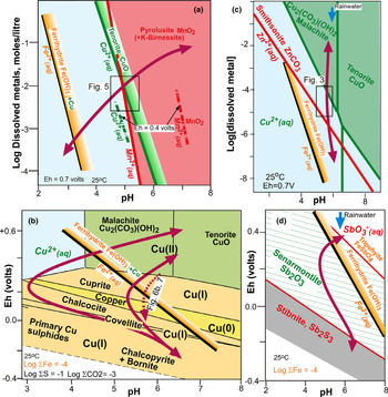
Ferrihydrite precipitates in oxidised Cu-bearing systems almost invariably contain some Cu that has been incorporated by adsorption of dissolved Cu2+ (Figs 1e; 6a). This adsorption may occur when ferrihydrite precipitates during neutralisation of acid solutions generated by bacterial oxidation of ferrous iron (Fig. 12a,b). Most trace metals are immobilised readily by adsorption onto ferrihydrite. The adsorption rate is dependent on both the type of metal cation and the pH of the system (Drever, Reference Drever1997; Langmuir, Reference Langmuir1997, Henne et al., Reference Henne, Craw, Gagen and Southam2019b). Adsorption of Cu to ferrihydrite precipitates can be enhanced by the typically large surface area of organo precipitates (Langmuir, Reference Langmuir1997; Loiselle et al., Reference Loiselle, McCraig, Dyar, Léveillé, Shieh and Southam2018) as well as by binding to functional groups (e.g. carboxyl) within such biologically mediated precipitates (Fariña et al., Reference Fariña, Peacock, Fiol, Antelo and Carvin2018). Negatively charged cell walls of individual bacteria and associated protein structures can also form nucleation sites and lead to very localised metal accumulations as in our examples from laboratory weathering experiments (e.g. Fig. 1a–f; Konhauser, Reference Konhauser1997). However, Cu is thermodynamically more soluble than Fe, especially under moderately acidic to alkaline conditions (Fig. 12a–c). Therefore, Cu can be more mobile and form separate precipitates in many surficial environments at a range of spatial scales, such as in our examples from surface discharge at the Mt Chalmers mine, the supergene zone at the Salobo IOCG mine, and our example of a manganese nodule from the ocean floor (Figs 3; 5; 10). Manganese has similar solubility to Cu under oxidised surficial conditions, so Cu and Mn can readily precipitate, either together, or in close proximity. Subtle biogeochemical fluctuations under circumneutral pH conditions, where Cu and Mn solubility boundaries have slightly different slopes (Fig. 12a), can apparently result in laminae with differing Cu and Mn contents at the 10 μm scale as seen in the supergene zone at Salobo and our manganese nodule example (Figs 5c; 10).
Geochemical models (from Geochemist's Workbench) showing relationships between dissolved metals and precipitates. Heavy arrows indicate typical environmental variations across equilibrium boundaries that lead to laminated precipitates. (a) Comparisons of solubility of Cu with Fe and Mn in oxidised environments (Eh = 0.7 V). Relative solubilities of Cu and Mn under more reducing conditions (Eh = 0.4 V) are indicated. (b) Eh–pH diagram for Cu. (c) Comparison of solubility of Cu with Zn and Fe in oxidised environments (Eh = 0.7 V). (d) Eh–pH diagram for Sb (for example in Fig. 4a–d).

Laminae with minerals of differing Cu oxidation states were examined in samples from the supergene zone at Salobo and reflect the progressive incursion of oxygen into more reduced settings, causing oxidation of the Cu and transformation of the mineralogy (Fig. 12b). Hence, boundaries between these mineral laminae are dynamic features that migrate progressively into more reduced environments, yielding laminated redox gradients on the millimetre scale or less (e.g. Figs 6b; 7c–f). It is also notable that in some surficial environments (e.g. the surface discharge at Mt Chalmers and the supergene zone at Mt Isa), there has been negligible incorporation of Mn within Cu precipitates (Figs 3b; 7), at least partly because Mn is more soluble than Cu under less-oxidised circumneutral pH conditions within such a redox gradient (Fig. 12a).
Minor incorporation of other transition metals into laminated metallic precipitates occurs principally in Cu- and Mn-rich laminae rather than Fe-rich laminae, reflecting the similar solubility of these minor metals to Cu and Mn under oxidised conditions. For example, co-precipitation of Zn with Cu is pronounced under the circumneutral conditions of neutralised AMD at Mt Chalmers (Fig. 3b; 12c). Similarly, Zn and Ni, and to a lesser extent Co, principally follow Cu and Mn during laminated manganese nodule formation, whereas greater Ti enrichment accompanies Fe deposition (Fig. 10b,c). However, Ti and V also accompany Cu and Mn in the subaerial weathering profile at Salobo (Fig. 5c) and some organisms (e.g. algae) are known for their metal-specific biosorption capacity (via ion exchange, complex formation and electrostatic interaction; Mata et al., Reference Mata, Blazquez, Ballester, Gonzalez and Munoz2008; Demirbas, Reference Demirbas2008; Zeraatkar et al., Reference Zeraatkar, Ahmadzadeh, Talebi, Moheimani and McHenry2016), which can further influence metal concentrations in laminae (e.g. a potential process in discharging waters at Mt Chalmers; Fig. 3).
Laminated precipitates related to gold deposits
Metalloids Sb and As are typically abundant around orogenic gold deposits (Craw and Kerr, Reference Craw and Kerr2017). Both these metalloids are variably soluble in the surficial environment and they are especially susceptible to variations in redox and pH conditions (Figs 12d; 13a). In both examples outlined in this paper (the Au–As–Sb orogenic deposit in Otago and the Waiuta orogenic gold mine), there is evidence for a wide range of redox conditions, from reduced sulfides to fully oxidised precipitates at sub-millimetre scales (Figs 2a,b; 4a–d). There is also textural evidence for biogeochemical fluctuations leading to complex mineralogical layering within these redox gradients (Figs 2a,b; 4a–d).
Eh–pH diagrams (from Geochemist's Workbench) showing redox relationships for: (a) As (for example in Fig. 2a,b); (b) Hg (for example in Fig. 2c,d); and (c) Au (for example in Fig. 9). Heavy arrows indicate typical environmental variations across equilibrium boundaries that lead to laminated precipitates.

The redox gradient developed on stibnite (Fig. 4a–d) is a result of similar weathering-driven progressive oxygen incursion to that observed on the native copper sample from Mt Isa (Fig. 7c–f). However, because of the young age and incipient nature of the weathering of the stibnite deposit, a more complete redox gradient has developed on a narrow spatial scale (Fig. 4a–d). Seasonal variations in rainfall and temperature undoubtedly had an effect on the biological effects on sulfide oxidation in the deposit, and also the effectiveness of physical incursion of oxidised rainwater. Localised bacterially mediated acidification from sulfide oxidation within the oxidising rock mass was countered by incursion of circumneutral rainwater and calcite in adjacent rocks during oxidation (Fig. 12d). The exact stability boundaries of tripuhyite are not known, but it is the most oxidised Sb–Fe mineral in this system coexisting with ferrihydrite (Fig. 4a; 12d). In contrast, textures of secondary stibnite (Fig. 4a–d) suggest that biologically mediated reduction of Sb and S has also occurred at times. Senarmontite crystals (Fig. 4a–c) attest to precipitation under intermediate redox stages that may have occurred during both oxidation and reduction (Fig. 12d).
Our As-bearing example from the Au–As–Sb orogenic sample (Fig. 2a,b; Table 1) also shows evidence for complex layering of both oxidation and reduction precipitates within the broad redox gradient defined by Fe(III)–As(V)-oxyhydroxide precipitates (Fig. 2a) that probably include ferrihydrite and scorodite (Fig. 13a) and the authigenic sulfide mineral realgar (Figs 2a,b; 13a). Arsenolite is an extremely soluble As mineral but dissolved As concentrations in this deposit reach very high levels, facilitating precipitation under intermediate redox conditions (Fig. 13a; Haffert et al., Reference Haffert, Sander, Hunter and Craw2010; Andrade et al., Reference Andrade, Jamieson, Kyser, Praharaj and Fortin2010), possibly during both oxidation and reduction stages. The most reduced end of the redox gradient is maintained by decomposing organic material. Dissolution of scorodite causes localised acidification, while incursion of oxygenated rainwater during frequent major rain events in the area can change pH and Eh (Fig. 13a; Davies et al., Reference Davies, Weber, Lindsay, Craw and Pope2011; Kerr et al., Reference Kerr, Craw, Pope and Trumm2018).
Mercury redistribution and associated laminations with varying Hg contents in the Waiuta sample (Fig. 2c,d) are caused by similar biochemical variations to As and Sb (Fig. 13b). In our dry-climate mine tailings example (Table 1), the deposit is highly oxidised and acidic because of biologically mediated sulfide oxidation that is on-going. Consequently, remnants of liquid Hg that were added to the tailings have generally been oxidised to schuetteite (Fig. 2c,d; 13b). However, carbonaceous material and relict sulfides in the deposit appear to cause local reduction and, locally, re-reduction of schuetteite to liquid Hg has occurred. (Fig. 2d; 13b).
Gold is mobile in the surficial environment where incipient oxidation of sulfide minerals yields metastable thiosulfate ions (S2O32–) that provide ligands for Au solubility at circumneutral pH (Fig. 13c; Webster, Reference Webster1986; Lengke and Southam, Reference Lengke and Southam2007). Decomposition of the thiosulfate ions over time, after further oxidation, and/or any acidification, results in gold deposition. In addition, gold can be mobilised with HS– ions as ligands under relatively reduced conditions in a narrow circumneutral pH band (Fig. 13c; Webster, Reference Webster1986). Hence, in a dynamic biogeochemical environment, gold can be dissolved and re-precipitated as a result of variations in pH, redox state, or both. In particular, bacterially mediated sulfide oxidation provides ideal biogeochemical gradients for gold redistribution (Fig. 13c; Reith et al., Reference Reith, Rogers, McPhail and Webb2006, Reference Reith, Lengke, Falconer, Craw and Southam2007, Reference Reith, Brugger, Zammit, Nies and Southam2013; Lengke and Southam, Reference Lengke and Southam2007; Johnston et al., Reference Johnston, Wyatt, Li, Ibrahim, Shuster, Southam and Magarvey2013; Shuster et al., Reference Shuster, Lengke, Marquez-Zavalia and Southam2016). Biogeochemical cycling that involves sulfide oxidation and episodic rainwater or groundwater incursion is therefore likely to result in laminated gold deposition and additions of authigenic gold to pre-existing gold particles (e.g. the Otago Schist sample pictured in Fig. 9a–d; 13c; Reith et al., Reference Reith, Rogers, McPhail and Webb2006, Reference Reith, Lengke, Falconer, Craw and Southam2007, Reference Reith, Brugger, Zammit, Gregg, Goldfarb, Andersen, DeSantis, Piceno, Brodie and Lu2012a, Reference Reith, Brugger, Zammit, Nies and Southam2013, Reference Reith, Falconer, Van Nostrand, Craw, Shuster and Wakelin2020).
Conclusions and implications
The mobility and (re)precipitation of metals in near-surface environments is driven primarily by geochemical disequilibrium, especially with respect to pH and redox states. Gradients in pH and redox conditions in rocks and associated shallow groundwaters develop on a range of spatial and temporal scales. These gradients are formed from, and subsequently affected by, complex interactions between biological and geological processes. Hence, different degrees of chemical disequilibrium arise on vast spatial (microenvironments to planetary) and temporal scales (days to millennia). Metalliferous mineral deposition results from subsequent supersaturation of waters that arise as a result of disequilibrium at the prevailing geochemical conditions. Changing conditions result in deposition of different minerals that reflect different degrees of supersaturation, leading to the formation of fine-scale laminations of metalliferous deposits.
In our examples, the biological component of these small near-surface settings with enhanced metal mobility is dominated by chemolithotrophic bacteria, such as Fe- and S-oxidisers and/or reducers. However, other entities such as archaea, algae, plants, mosses, fungi and microinvertebrates can also affect the biogeochemistry of natural systems. Sulfur- and Fe-oxidising bacteria are common chemolithotrophs that affect sulfide-bearing metal deposits because of the influence of nearby air and oxygenated shallow groundwater. However, localised reductive environments can develop around decaying organic material and/or partially decomposed sulfide minerals, thereby, enabling reducing bacteria to play a role in the development of complex redox gradients in such settings. Biological entities that are not actively oxidising or reducing metals, can be relatively passive occupants of these metalliferous environments, and merely provide substrates with large surface area for deposition of precipitates. Bacteria can also take passive advantage of on-going mineral reactions driven by geochemical disequilibrium and can contribute to those reactions by catalysing the kinetic reaction rates. In doing so, the metabolic processes of bacteria can cause localised changes to the biogeochemical environments, especially with respect to pH and redox conditions that can lead to metal dissolution and/or metal deposition.
The laminated metalliferous deposits outlined in this paper have complex biogeochemical parageneses, which are not predictable because there are many varied parameters that affect their respective formation. However, some generalisations can be made. For example, there is commonly a spatial separation of Fe-rich precipitates from those with Cu and Mn because of the greater solubility of the latter metals under weakly acidic and oxidised conditions. Other transition metals such as Ni, V and Zn also follow Cu and Mn rather than Fe. In contrast, metalloids As and Sb have a strong affinity for Fe under oxidising conditions, but not under more reduced conditions. There is, however, inevitably some overlap between these general trends.
The laminated deposits described in this paper are small, but they reflect the types of biogeochemical processes that can pervade all near-surface environments. The textures, mineral species, and metal associations within these deposits are likely to be encountered in all facets of mineral deposit development: initial exploration activity of near-surface locations; mining of shallow portions of orebodies, especially supergene zones; and in downstream environmental issues with respect to discharging metalliferous waters.
Acknowledgements
Parts of this research were funded by the Australian Research Council Linkage Programs LP140100804 and LP140100805, and parts were supported by the Royal Society of New Zealand via the Marsden Fund. Many of the images and associated data were obtained from the XFM beamline at the Australian Synchrotron, part of ANSTO, in Melbourne, Australia. Some SEM work was carried out at the Centre for Microscopy and Microanalysis at the University of Queensland, where we thank Ron Rasch and Kim Sewell for their excellent support. Additional SEM work was carried out at Otago Micro and Nanoscale Imaging (OMNI), University of Otago, with able assistance of Kat Lilley. Field work to collect rocks and bacterial ecosystems in Brazil was supported by the mining staff from the Vale Salobo mine. Field work to collect bacterial ecosystems from Mount Chalmers in Queensland was funded and supported by the Department of Natural Resources, Mines and Energy in Queensland. Manganese nodule samples were supplied by Simon Richards from Adrok Ltd.